The convergence rate of the equilibrium measure for the hybrid LQG Mean Field Game

Abstract.

In this work, we study the convergence rate of the $N$-player LQG game with a Markov chain common noise towards its asymptotic Mean Field Game. By postulating a Markovian structure via two auxiliary processes for the first and second moments of the Mean Field Game equilibrium and applying the fixed point condition in Mean Field Game, we first provide the characterization of the equilibrium measure in Mean Field Game with a finite-dimensional Riccati system of ODEs. Additionally, with an explicit coupling of the optimal trajectory of the $N$-player game driven by $N$ dimensional Brownian motion and Mean Field Game counterpart driven by one-dimensional Brownian motion, we obtain the convergence rate $O(N^{-1/2})$ with respect to 2-Wasserstein distance.

Keywords. Convergence rate, Mean Field Games, Common noise

AMS subject classifications. 91A16, 93E20

1. Introduction

Mean Field Game (MFG) theory is intended to describe an asymptotic limit of complex $N$-player differential game invariant to a reshuffling of the players’ indices, and has attracted resurgent attention from numerous researchers in probability after its pioneering works of [20, Lasry and Lions] and [16, Huang, Caines, and Malhame], and we refer to comprehensive descriptions to the book [7, Carmona and Delarue] and the references therein.

In this paper, we study the convergence rate of equilibrium measures of $N$-player differential game in the context of Linear-Quadratic (LQ) structure with a common noise to its limiting MFG system. Different from the works mentioned above, the common noise in this paper is a continuous-time Markov chain (CTMC) instead of Brownian motion, which often models the real-world control problems associated with hybrid systems. Markov chains are widely used to model systems that exhibit randomness and transition between different states. In various real-world scenarios, especially in economics (see [27]), finance (see [30]), biology (see [31]), and engineering (see [29]), the dynamics of systems can be effectively represented as discrete states with probabilistic transitions between them. By using CTMC, the applications aim to model less frequently changing common noises, such as government policies implemented by two different regimes.

LQ control problems have been widely recognized in the stochastic control theory due to their broad applications. More importantly, LQ structure leads to solvability in a closed form, namely the Ricatti system, and this usually sheds light on many fundamental properties of the control theory. For this reason, LQ structure has also been studied in MFGs with or without common noises for its importance. The related literature include major and minor LQG Mean Field Games system ([14, 23, 9]); social optimal in LQG Mean Field Games ([15, 8]); the LQG Mean Field Games with different model settings ([3, 12, 4, 13]); and LQG Graphon Mean Field Games ([11]). Recently, LQ Mean Field Games with a Brownian motion as the common noise have also been studied in ([1, 26]) with restrictions of the dependence of measure on its mean alone. Moreover, some literature considers various topics of Mean Field control and game problems with Markov chain common noise, see [21, 24, 25].

A fundamental question in this regard is the convergence rate of $N$-player game to the desired MFG system. A well-known result is about the convergence rate of value functions of the generic player, which can be shown $O(N^{-1})$, see for instance [5, 6, 7, 17]. In particular, [17] establishes the convergence rate of value functions in the sense of

$$J_{1}^{N}(\hat{\alpha}_{1},\hat{\alpha}_{-1})\leq J_{1}^{N}(\alpha_{1},\hat{\alpha}_{-1})+O(N^{-1}),$$

where $J_{1}^{N}$ is the value of the first player in $N$-player game and $\hat{\alpha}$ is the Nash equilibrium decentralized control process for the Mean Field Game problem.

In contrast, the convergence rate of equilibrium measures is another challenging question due to the complication of the correlation structures among $N$ players. To be more concrete, we examine the behavior of the $\hat{X}_{it}^{(N)}$, who represents the equilibrium state of the $i$-th player at time $t$ in the $N$-player game defined within the probability space $\left(\Omega^{(N)},\mathcal{F}^{(N)},\mathbb{F}^{(N)},\mathbb{P}^{(N)}\right)$. Additionally, we denote $\hat{X}_{t}$ as the equilibrium path at time $t$ derived from the associated MFG defined in the probability space $(\Omega,\mathcal{F},\mathbb{F},\mathbb{P})$. The question pertains to the convergence of $\hat{X}_{1t}^{(N)}$ as follows:

• The $\mathbb{W}_{p}$-convergence rate of the representative equilibrium path,

  $$\mathbb{W}_{p}\left(\mathcal{L}\left(\hat{X}_{1t}^{(N)}\right),\mathcal{L}\left(\hat{X}_{t}\right)\right)=O\left(N^{-?}\right).$$

  Here, $\mathbb{W}_{p}$ denotes the $p$-Wasserstein metric.

The existing literature extensively explores the convergence rate in this context. For (Q), Theorem 2.4.9 of the monograph [6] establishes a convergence rate of $O(N^{-1/2})$ using the $\mathbb{W}_{1}$ metric. More recently, [18] addresses (Q) by introducing displacement monotonicity and controlled common noise, and Theorem 2.23 applies the maximum principle of forward-backward propagation of chaos to achieve the same convergence rate. It is important to note that these results are not applicable to the Linear Quadratic Gaussian (LQG) framework, primarily due to the assumption concerning the linear growth of the cost functional.

The main result of this paper establishes that the equilibrium measures exhibit a convergence rate of $1/2$ concerning the 2-Wasserstein distance. The precise statement of this result can be found in Theorem 6. In comparison to the aforementioned literature, two primary distinctions emerge. Firstly, within the framework of Mean Field Games, the common noise is modeled as a Continuous-Time Markov Chain. Secondly, a significant difference lies in the cost function’s behavior, as it does not possess linear growth within the context of the Linear Quadratic Gaussian (LQG) framework.

To obtain the desired convergence rate in this paper, the first building block is the characterization of the equilibrium measure of the limiting MFG by a finite-dimensional ODE system. The key step leading us to a desired finite-dimensional system is that, instead of searching for the infinite-dimensional function directly, we postulate a Markovian structure via auxiliary processes (15) governed by its finite-dimensional coefficient functions, which exhibits the distinct feature of Markov chain common noise relatives to the Brownian motion counterpart.

The next stage towards the convergence rate is to compare the limiting MFG system to a $N$-player game. In contrast to the characterization of the MFG system, it is relatively routine to solve the $N$-player game due to its LQ structure. Therefore, the convergence rate problem can be recasted to the following question about a coupling of the two following processes: For two equilibrium processes $\hat{X}$ of MFG in $\Omega$ and $\hat{X}_{1}^{(N)}$ of $N$-player game in $\Omega^{(N)}$, finding a random process $Z^{N}$ in $\Omega$ whose distribution is identical to $\hat{X}_{1}^{(N)}$ satisfying the estimate in the form of $\mathbb{E}[|\hat{X}_{t}-Z^{N}_{t}|^{2}]=O\left(N^{-?}\right).$ For this purpose, we first show an $N$-invariant algebraic structure of the seemingly intractable $\kappa N^{3}$ dimensional ODE system (27), which originated from [17, Huang and Yang] as a dimensional reduction in the system with Brownian common noise. Thanks to this $N$-invariant structure, the complex ODE system (27) can be reduced to the ODE system (31) whose dimension agrees with the ODE (12) of MFG system. Moreover, $\hat{X}_{1}^{(N)}$ can be represented as a stochastic flow driven by two Brownian motions $W_{1}^{(N)}$ and $W_{-1}^{(N)}:=\frac{1}{\sqrt{N-1}}\sum_{i=2}^{N}W_{i}^{(N)}$, which enables us to embed the equilibrium process $\hat{X}_{1}^{(N)}$ to any probability space having only two Brownian motions.

The rest of this paper is outlined as follows: Section 2 presents a precise formulation of the problem and two main results. Section 3 is devoted to the derivation of our first result: the equilibrium of MFGs. In Section 4, we show in detail the convergence of the $N$-player game to MFGs, which yields our second main result. Section 5 demonstrates the convergence by some numerical examples. The conclusion and some possible future works are summarised in Section 6. Section 7 is an appendix that collects some related facts to support our main theme.

2. Problem setup and Main results

First, we collect common notations used in this paper in Subsection 2.1. Then, we set up problems on MFGs and the $N$-player game separately in Subsections 2.2 and 2.3. The main results are presented in Subsection 2.4 and some interpretations of our main results are added in Subsection 2.5.

2.1. Notations

Let $T>0$ be a fixed terminal time and $(\Omega,\mathcal{F}_{T},\mathbb{F}=\{\mathcal{F}_{t}:0\leq t\leq T\},\mathbb{P})$ be a completed filtered probability space satisfying the usual conditions, on which $W$ and $B$ are two independent standard Brownian motions, and $Y$ is a continuous time Markov chain (CTMC) independent of $(W,B)$ taking values in a finite state space $\mathcal{Y}=\{1,2,\dots,\kappa\}$ with a generator

$$Q=(q_{i,j})_{i,j\in\mathcal{Y}}$$ (1)

satisfying $q_{i,j}\geq 0$ for all $i\neq j\in\mathcal{Y}$ and $\sum_{i\neq j}q_{i,j}+q_{i,i}=0$ for each $i\in\mathcal{Y}$. In the above, the Brownian motion $B$ does not play any role in MFG problem formulation until the convergence proof of the $N$-player game to MFGs.

By $L^{p}:=L^{p}(\Omega,\mathbb{P})$, we denote the space of random variables $X$ on $(\Omega,\mathcal{F}_{T},\mathbb{P})$ with finite $p$-th moment with norm $\|X\|_{p}=(\mathbb{E}\left[|X|^{p}\right])^{1/p}$. We also denote by $L_{\mathbb{F}}^{p}:=L_{\mathbb{F}}^{p}([0,T]\times\Omega)$ the space of all $\mathbb{F}$-progressively measurable random processes $\alpha=(\alpha_{t})_{0\leq t\leq T}$ satisfying

$$\mathbb{E}\left[\int_{0}^{T}|\alpha_{t}|^{p}dt\right]<\infty.$$

For any polish (complete separable metric) space $(P,\mathcal{B}(P),d)$, we use $\delta_{x}$ to denote the Dirac measure on the point $x\in P$. Then, the collection of all probabilities $m$ on $(P,\mathcal{B}(P),d)$ having finite $k$-th moment is denoted by $\mathcal{P}_{k}(P)$, i.e.

$$[m]_{k}:=\int x^{k}m(dx)<\infty,\quad\forall m\in\mathcal{P}_{k}(P).$$

The equilibrium of MFGs with the common noise yields the conditional distribution. For real-valued random variables $X$ and $Z$ in $(\Omega,\mathcal{F}_{T},\mathbb{P})$, we denote the distribution of $X$ conditional on $\sigma(Z)$ by $\mathcal{L}(X|Z)$, or equivalently

$$\mathcal{L}(X|Z)(A)=\mathbb{E}[I_{A}(X)|Z],\quad\forall A\in\mathcal{F}_{T}.$$

Note that $\mathcal{L}(X|Z)(A):\Omega\mapsto\mathbb{R}$ is a $\sigma(Z)$-measurable random variable, therefore, $\mathcal{L}(X|Z)$ is $\sigma(Z)$-measurable random probability distribution with $k$-th moment $[\mathcal{L}(X|Z)]_{k}=\mathbb{E}[X^{k}|Z]$, if it exists. We refer to more details on the conditional distribution in Volume II of [7]. The next proposition provides an embedding approach to prove a convergence in distribution, which will be used later in the convergence of the $N$-player game to MFGs.

Proposition 1.

Suppose $(\Omega^{(N)},\mathcal{F}_{T}^{(N)},\mathbb{P}^{(N)})$ is a complete probability space. Let $X^{(N)}$ and $X$ be random variables of $\Omega^{(N)}\mapsto P$ and $\Omega\mapsto P$, respectively. Then, $X^{(N)}$ is convergent in distribution to $X$, denoted by $X^{(N)}\Rightarrow X$, if there exists $Z^{N}:\Omega\mapsto P$ satisfying $\mathcal{L}(Z^{N})=\mathcal{L}(X^{(N)})$, such that $Z^{N}\to X$ holds almost surely, i.e.

$$\lim_{N\to\infty}d(Z^{N},X)=0,\hbox{ almost surely in }\mathbb{P},$$

where $d$ represents the metric assigned to the space $P$.

In this paper, we formulate the $N$-player game in the completed filtered probability space

$$(\Omega^{(N)},\mathcal{F}_{T}^{(N)},\mathbb{F}^{(N)}:=\{\mathcal{F}_{t}^{(N)}:0\leq t\leq T\},\mathbb{P}^{(N)}),$$

and $Y^{(N)}$ is the continuous time Markov chain in $\Omega^{(N)}$ with the same generator given by (1) and $W^{(N)}=(W^{(N)}_{i}:i=1,2,\dots,N)$ is an $N$-dimensional standard Brownian motion. We assume $Y^{(N)}$ and $W^{(N)}$ are independent of each other.

For better clarity, we use the superscript $(N)$ for a random variable to emphasize the probability space $\Omega^{(N)}$ it belongs to. For example, Proposition 1 denotes a random variable in $\Omega^{(N)}$ by $X^{(N)}$, while its distribution copy in $\Omega$ by $Z^{N}$, but not by $Z^{(N)}$.

2.2. The equilibrium of MFGs

In this section, we define the equilibrium of MFGs associated with a generic player’s stochastic control problem in the probability setting $\Omega$, see Section 2.1.

Given a random measure flow $m:(0,T]\times\Omega\mapsto\mathcal{P}_{2}(\mathbb{R})$, consider a generic player who wants to minimize her expected accumulated cost on $[0,T]$:

$$\begin{array}[]{ll}J(y,x,\alpha)=\displaystyle\mathbb{E}\left[\int_{0}^{T}\left(\frac{1}{2}\alpha_{s}^{2}+F(Y_{s},X_{s},m_{s})\right)ds+G(Y_{T},X_{T},m_{T})\Big{|}Y_{0}=y,X_{0}=x\right]\end{array}$$ (2)

with some given cost functions $F,G:\mathcal{Y}\times\mathbb{R}\times\mathcal{P}_{2}(\mathbb{R})\mapsto\mathbb{R}$ and underlying random processes $(Y,X):[0,T]\times\Omega\mapsto\mathcal{Y}\times\mathbb{R}$. Among three processes $(Y,X,m)$, the generic player can control the process $X$ via $\alpha$ in the form of

$$X_{t}=X_{0}+\int_{0}^{t}\left(\tilde{b}_{1}(Y_{s},s)X_{s}+\tilde{b}_{2}(Y_{s},s)\alpha_{s}\right)ds+W_{t},\quad\forall t\in[0,T],$$ (3)

where $\tilde{b}_{1}(\cdot,\cdot)$ and $\tilde{b}_{2}(\cdot,\cdot)$ are two deterministic functions. We assume that the initial state $X_{0}$ is independent of $Y$. The Brownian motion $W$ is the individual noise of the generic player, the process $Y$ of (1) represents the common noise, and $m=(m_{t})_{0\leq t\leq T}$ is a given random density flow normalized up to total mass one.

The objective of the control problem for the generic player is to find its optimal control $\hat{\alpha}\in\mathcal{A}:=L^{4}_{\mathbb{F}}$ to minimize the total cost, i.e.

$$V[m](y,x)=J[m](y,x,\hat{\alpha})\leq J[m](y,x,\alpha),\quad\forall\alpha\in\mathcal{A}.$$ (4)

Associated with the optimal control $\hat{\alpha}$, we denote the optimal path by $\hat{X}=(\hat{X}_{t})_{0\leq t\leq T}$. To introduce MFG Nash equilibrium, it is often convenient to highlight the dependence of the optimal path and optimal control of the generic player and its associated value on the underlying density flow $m$, which are denoted by

$$\hat{X}_{t}[m],\hat{\alpha}_{t}[m],\hbox{ and }V[m],$$

respectively. Now, we present the definition of the equilibrium below, see also Volume II-P127 of [7] for a general setup with a common noise.

Definition 2.

Given an initial distribution $\mathcal{L}(X_{0})=m_{0}\in\mathcal{P}_{2}(\mathbb{R})$, a random measure flow $\hat{m}=\hat{m}(m_{0})$ is said to be an MFG equilibrium measure if it satisfies the fixed point condition

$$\hat{m}_{t}=\mathcal{L}(\hat{X}_{t}[\hat{m}]|Y),\ \forall 0<t\leq T,\ \hbox{ almost surely in }\mathbb{P}.$$ (5)

The path $\hat{X}$ and the control $\hat{\alpha}$ associated to $\hat{m}$ is called the MFG equilibrium path and equilibrium control, respectively. The value function of the control problem associated with the equilibrium measure $\hat{m}$ is called as MFG value function, denoted by

$$U(m_{0},y,x)=V[\hat{m}](y,x).$$ (6)

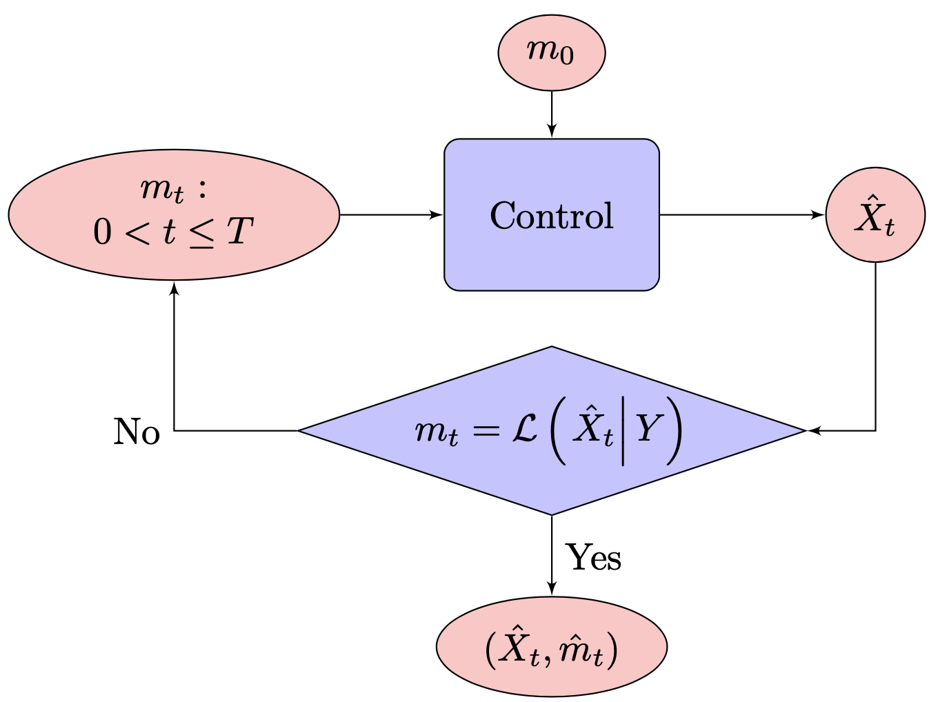
Figure 1. MFGs diagram.

The flowchart of MFGs diagram is given in Figure 1. It is noted from the optimality condition (4) and the fixed point condition (5) that

$$J[\hat{m}](y,x,\hat{\alpha})\leq J[\hat{m}](y,x,\alpha),\quad\forall\alpha$$

holds for the equilibrium measure $\hat{m}$ and its associated equilibrium control $\hat{\alpha}$, while it is not

$$J[\hat{m}](y,x,\hat{\alpha})\leq J[m](y,x,\alpha),\quad\forall\alpha,m.$$

Otherwise, this problem turns into a McKean-Vlasov control problem discussed in [24]. Furthermore, it’s important to note that the Continuous-Time Markov Chain $Y$ serves a role as common noise. This is due to the fact that the mean field term is conditioned on the distribution of $Y$.

2.3. Equilibrium of the $N$-player game

The discrete counterpart of MFGs is an $N$-player game, which is formulated below in the probability space $\Omega^{(N)}$, see Section 2.1 for more details on the probability setup.

Recall that, $W_{it}^{(N)}$ and $W_{jt}^{(N)}$ are independent Brownian motions for $j\neq i$ and they are called individual noises in the $N$-player game. The common noise $Y^{(N)}$ is the continuous time Markov chain in $\Omega^{(N)}$ with the generator given by (1). Let the player $i$ follow the dynamic, for $i=1,2,\dots,N$,

$$dX_{it}^{(N)}=\left(\tilde{b}_{1}(Y_{t}^{(N)},t)X_{it}^{(N)}+\tilde{b}_{2}(Y_{t}^{(N)},t)\alpha_{it}^{(N)}\right)dt+dW_{it}^{(N)},\quad X_{i0}^{(N)}=x^{(N)}_{i}.$$ (7)

The cost function for player $i$ associated to the control $\alpha^{(N)}=(\alpha_{i}^{(N)}:i=1,2,\dots,N)$ is

$$J_{i}^{N}(y,x^{(N)},\alpha^{(N)}) =\mathbb{E}\left[\int_{0}^{T}\left(\frac{1}{2}|\alpha_{it}^{(N)}|^{2}+F(Y_{t}^{(N)},X_{it}^{(N)},\rho(X_{t}^{(N)}))\right)dt+\right.$$ (8)

$$\hskip 72.26999pt\left.G(Y_{T}^{(N)},X_{iT}^{(N)},\rho(X_{T}^{(N)}))\Big{|}X_{0}^{(N)}=x^{(N)},Y_{0}^{(N)}=y\right],$$

where $x^{(N)}=(x_{1}^{(N)},x_{2}^{(N)},\dots,x_{N}^{(N)})$ is an $\mathbb{R}^{N}$-valued random vector in $\Omega^{(N)}$ to denote the initial state for $N$ player, $\alpha_{i}^{(N)}\in\mathcal{A}^{(N)}:=L_{\mathbb{F}^{(N)}}^{4}$, and

$$\rho(x^{(N)})=\frac{1}{N}\sum_{i=1}^{N}\delta_{x_{i}^{(N)}}$$

is the empirical measure of a vector $x^{(N)}$ with Dirac measure $\delta$. We use the notation for the control $\alpha^{(N)}=(\alpha_{i}^{(N)},\alpha_{-i}^{(N)})=(\alpha_{1}^{(N)},\alpha_{2}^{(N)},\ldots,\alpha_{N}^{(N)})$.

Definition 3.

1. The value function of player $i$ for $i=1,2,\ldots,N$ of the Nash game is defined by $V^{N}=(V^{N}_{i}:i=1,2,\ldots,N)$ satisfying the equilibrium condition

   $$\begin{array}[]{ll}V_{i}^{N}(y,x^{(N)})&=J_{i}^{N}(y,x^{(N)},\hat{\alpha}_{i}^{(N)},\hat{\alpha}_{-i}^{(N)})\leq J_{i}^{N}(y,x^{(N)},\alpha_{i}^{(N)},\ \hat{\alpha}_{-i}^{(N)}),\quad\forall\alpha_{i}^{(N)}\in\mathcal{A}^{(N)}.\end{array}$$ (9)

2. The equilibrium path of the $N$-player game is the random path $\hat{X}_{t}^{(N)}=(\hat{X}_{1t}^{(N)},X_{2t}^{(N)},\dots,\hat{X}_{Nt}^{(N)})$ driven by (7) associated to the control $\hat{\alpha}_{t}^{(N)}$ satisfying the equilibrium condition of (9).

2.4. The main result with quadratic cost structures

We consider the following two functions $F,G:\mathcal{Y}\times\mathbb{R}\times\mathcal{P}_{2}(\mathbb{R})\mapsto\mathbb{R}$ in the cost functional (2):

$$F(y,x,m)=h(y)\int_{\mathbb{R}}(x-z)^{2}m(dz),$$ (10)

and

$$G(y,x,m)=g(y)\int_{\mathbb{R}}(x-z)^{2}m(dz),$$ (11)

for some $h,g:\mathcal{Y}\mapsto\mathbb{R}^{+}$. In this case, the $F$ and $G$ terms in (8) of the $N$-player game can be written by

$$F(Y_{t}^{(N)},X_{it}^{(N)},\rho(X_{t}^{(N)}))=\frac{h(Y_{t}^{(N)})}{N}\sum_{j=1}^{N}(X_{it}^{(N)}-X_{jt}^{(N)})^{2},$$

and

$$G(Y_{T}^{(N)},X_{iT}^{(N)},\rho(X_{T}^{(N)}))=\frac{g(Y_{T}^{(N)})}{N}\sum_{j=1}^{N}(X_{iT}^{(N)}-X_{jT}^{(N)})^{2},$$

respectively.

Remark 4.

First, we note that $F$ and $G$ possess the quadratic structures in $x$. Secondly, the coefficients $h(y)$ and $g(y)$ provide the sensitivity to the mean field effects, which depend on the current CTMC state. For another remark, let us consider the scenario where the number of states is $2$ and sensitivities are invariant, say

$$h(0)=h(1)=h,\ g(0)=g(1)=0.$$

Then the cost function and hence the entire problem is free from the common noise. Interestingly, as shown in the Appendix 7.1, there is no global solution for MFGs when $h<0$, while there is a global solution when $h>0$.

Moreover, the uniqueness of Mean Field Game can be achieved under the displacement monotonicity condition. It is easy to check that (10)-(11) satisfy the displacement monotonicity condition. Note that

$$F_{x}(y,x,m)=2h(y)(x-[m]_{1}),\quad G_{x}(y,x,m)=2g(y)(x-[m]_{1}),$$

which gives that

$$\mathbb{E}\left[\left(F_{x}(y,X_{1},m_{X_{1}})-F_{x}(y,X_{2},m_{X_{2}})\right)(X_{1}-X_{2})\right]=2h(y)\left(\mathbb{E}\left[\left(X_{1}-X_{2}\right)^{2}\right]-\left(\mathbb{E}[X_{1}]-\mathbb{E}[X_{2}]\right)^{2}\right)\geq 0$$

for all $y\in\mathcal{Y}$ if $h>0$ on $\mathcal{Y}$, where $m_{X_{1}}$ and $m_{X_{2}}$ is the law of $X_{1}$ and $X_{2}$ respectively. Similarly, we can obtain that

$$\mathbb{E}\left[\left(G_{x}(y,X_{1},m_{X_{1}})-G_{x}(y,X_{2},m_{X_{2}})\right)(X_{1}-X_{2})\right]\geq 0$$

for all $y\in\mathcal{Y}$ if $g>0$ on $\mathcal{Y}$. Therefore, we require positive values for all sensitivities for simplicity. It is of course an interesting problem to investigate the explosion when some sensitivities are negative.

Wrapping up the above discussions, we impose the following assumptions:

• $\tilde{b}_{1}(y,\cdot),\tilde{b}_{2}(y,\cdot):[0,T]\mapsto\mathbb{R}$ are continuous functions for all $y\in\mathcal{Y}$.

• The cost functions are given by (10)-(11) with $h,g>0$; The initial $X_{0}$ of MFGs satisfies $\mathbb{E}[X_{0}^{2}]<\infty$.

• In addition to (A1), the initial $x^{(N)}=(x_{1}^{(N)},x_{2}^{(N)},\dots,x_{N}^{(N)})$ of the $N$-player game is a vector of i.i.d. random variables in $\Omega^{(N)}$ with the same distribution as the initial $\mathcal{L}(X_{0})$ of MFG.

Our objective for this paper is to understand the Nash equilibrium of MFGs and its connection to the $N$-player game equilibrium:

• With Assumptions (A0), (A1), and (A2), obtain the convergence rate of $(\hat{X}_{1t}^{(N)},Y^{(N)})$ from the $N$-player game of Definition 3 to $(\hat{X}_{t},Y)$ from MFGs of Definition 2 in distribution.

To answer (P1), it is critical to have a solid understanding of the joint distribution $(\hat{X}_{t},Y)$ for the underlying MFG, which yields another question:

• With Assumptions (A0) and (A1), characterize the MFG equilibrium path $\hat{X}$, as well as associated equilibrium measure $\hat{m}$ along the Definition 2;

For our first main result, we first answer (P2) via the following Riccati system for unknowns $(a_{y},b_{y},c_{y},k_{y}:y\in\mathcal{Y})$:

$$\begin{cases}\displaystyle a_{y}^{\prime}+2\tilde{b}_{1y}a_{y}-2\tilde{b}^{2}_{2y}a_{y}^{2}+\sum_{i=1}^{\kappa}q_{y,i}a_{i}+h_{y}=0,\\ \displaystyle b_{y}^{\prime}+\left(2\tilde{b}_{1y}-4\tilde{b}^{2}_{2y}a_{y}\right)b_{y}+\sum_{i=1}^{\kappa}q_{y,i}b_{i}+h_{y}=0,\\ \displaystyle c_{y}^{\prime}+a_{y}+b_{y}+\sum_{i=1}^{\kappa}q_{y,i}c_{i}=0,\\ \displaystyle k_{y}^{\prime}-2\tilde{b}^{2}_{2y}a_{y}^{2}+4\tilde{b}^{2}_{2y}a_{y}b_{y}+2\tilde{b}_{1y}k_{y}+\sum_{i=1}^{\kappa}q_{y,i}k_{i}=0,\\ \displaystyle a_{y}(T)=b_{y}(T)=g_{y}\text{ , }c_{y}(T)=k_{y}(T)=0,\end{cases}$$ (12)

where $h_{y}=h(y),\,g_{y}=g(y)$ for $y\in\mathcal{Y}$. Next, we present our first main result about the equilibrium path, the equilibrium control, and the value function in MFG.

Theorem 5 (MFG).

Under (A0)-(A1), there exists a unique solution $(a_{y},b_{y},c_{y},k_{y}:y\in\mathcal{Y})$ for the Riccati system (12). With these solutions, the MFG equilibrium path $\hat{X}=\hat{X}[\hat{m}]$ is given by

$$d\hat{X}_{t}=\left(\tilde{b}_{1}(Y_{t},t)\hat{X}_{t}-2\tilde{b}_{2}^{2}(Y_{t},t)a_{Y_{t}}(t)\left(\hat{X}_{t}-\hat{\mu}_{t}\right)\right)dt+dW_{t},\quad\hat{X}_{0}=X_{0},$$ (13)

with equilibrium control

$$\hat{\alpha}_{t}=-2\tilde{b}_{2}(Y_{t},t)a_{Y_{t}}(t)\left(\hat{X}_{t}-\hat{\mu}_{t}\right),$$ (14)

where

$$d\hat{\mu}_{t}=\tilde{b}_{1}(Y_{t},t)\hat{\mu}_{t}dt,\quad\hat{\mu}_{0}=\mathbb{E}[X_{0}].$$

Moreover, the value function $U$ is

$$U(m_{0},y,x)=a_{y}(0)x^{2}{-2a_{y}(0)x[m_{0}]_{1}+k_{y}(0)[m_{0}]_{1}^{2}}+b_{y}(0)[m_{0}]_{2}+c_{y}(0),\quad y\in\mathcal{Y}.$$

The proof of theorem 5 is based on the Markovian structure of the equilibrium and the fixed point condition of the MFG problem, and it is provided in Subsection 3.3. The next theorem establishes the convergence result and answers the problem (P1) with the convergence rate $\frac{1}{2}$.

Theorem 6 (Convergence rate).

Under Assumptions (A0)-(A1)-(A2), the joint law $(\hat{X}_{1t}^{(N)},Y_{t}^{(N)})$ of the $N$-player game converges in distribution to that of the MFG equilibrium $(\hat{X}_{t},Y_{t})$ for any $t\in(0,T]$ at the convergence rate

$$\mathbb{W}_{2}\left(\mathcal{L}(\hat{X}_{1t}^{(N)},Y_{t}^{(N)}),\mathcal{L}(\hat{X}_{t},Y_{t})\right)=O\left(N^{-\frac{1}{2}}\right),\quad\hbox{ as }N\to\infty.$$

The proof of Theorem 6 is given in Subsection 4.3 since it needs the comparison between the equilibrium path $\hat{X}_{1t}^{(N)}$ in $N$-player game and the equilibrium path $\hat{X}_{t}$ in MFG.

2.5. Remarks on the main results

One can interpret the main results in plain words: For $N$-player game with dynamic (7) and cost structure (8) for large $N$, the equilibrium control of the generic player can be effectively approximated by steering itself toward the population center $\hat{\mu}_{t}$ depending only on the function $\tilde{b}_{1}(\cdot)$ and the entire past of the common noise, whose velocity is dependent on only the function $\tilde{b}_{2}(\cdot)$ and the entire past of the common noise. The effectiveness can be quantified by the convergence rate of $1/2$ for the one-dimensional Mean Field Game under LQ structure and CMTC common noise. A natural question is whether the convergence rate can be generalized to more general settings.

This paper focuses on the one-dimensional problem to avoid unnecessary symbol complexity. Therefore, the main convergence rate $1/2$ still holds for multidimensional problems using the same coupling procedure. For convenience to check, we summarize the computation involved in multidimensional problems in Appendix 7.5.

The current coupling procedure can also be adapted with suitable modifications to the LQ Mean Field Game problems with Brownian common noise, see [19]. In particular, the reduction of the $O(N^{3})$-dimensional ODE can be conducted similarly and the convergence rate is still maintained as $1/2$. However, the dependence of the mean and variance process on the common noise and subsequent calculations are significantly different from the current paper, see Definition 4 of [19].

Indeed, choosing the CTMC common noise instead of Brownian motion does not simplify the underlying problem, since it preserves the path-dependence feature of the equilibrium measure. On the contrary, the advantage of CTMC common noise is that the applications aim to model less frequently changing environment settings, such as government policies implemented by multiple different regimes. Due to its realistic applications, stochastic control theory perturbed by CTMC is extensively studied in the context of hybrid control problems, see books [22, 28] and the references therein.

We close this section with a remark on the uniqueness. The uniqueness of Mean Field Game can be achieved under Lasry-Lions monotonicity [20] or displacement monotonicity [10] and our setting in Section 2.2 satisfies the displacement monotonicity. Thus, the convergence of Theorem 6 implies that the unique equilibrium path of $N$-player game converges to the unique equilibrium paths of the limiting MFG, which is characterized by Theorem 5.

3. Main results of MFG

This section is devoted to the proof of the first main result Theorem 5 on the MFG solution. First, we outline the scheme based on the Markovian structure of the equilibrium by reformulating the MFG problem in Subsection 3.1. Next, we solve the underlying control problem in Subsection 3.2 and provide the corresponding Riccati system. Finally, Subsection 3.3 proves Theorem 5 by checking the fixed point condition of MFG problem.

3.1. Overview

By Definition 3, to solve for the equilibrium measure, one shall search the infinite dimensional space of the random measure flows $m:(0,T]\times\Omega\mapsto\mathcal{P}_{2}(\mathbb{R})$, until a measure flow satisfies the fixed point condition $m_{t}=\mathcal{L}(\hat{X}_{t}|Y),\forall t\in(0,T]$, see Figure 1, which requires to check the following infinitely many conditions:

$$[m_{t}]_{k}=\mathbb{E}[\hat{X}^{k}_{t}|Y],\quad\forall k=1,2,\ldots,$$

if they exist.

The first observation is that the cost functions $F$ and $G$ in (10)-(11) are dependent on the measure $m$ only via the first two moments:

$$F(y,x,m) =h(y)(x^{2}-2x[m]_{1}+[m]_{2}),$$

$$G(y,x,m) =g(y)(x^{2}-2x[m]_{1}+[m]_{2}).$$

Therefore, the underlying stochastic control problem for MFGs can be entirely determined by the input given by $\mathbb{R}^{2}$ valued random process $\mu_{t}=[m_{t}]_{1}$ and $\nu_{t}=[m_{t}]_{2}$, which implies that the fixed point condition can be effectively reduced to check two conditions only:

$$\mu_{t}=\mathbb{E}[\hat{X}_{t}|Y],\ \nu_{t}=\mathbb{E}[\hat{X}_{t}^{2}|Y].$$

This observation effectively reduces our search from the space of random measure-valued processes $m:(0,T]\times\Omega\mapsto\mathcal{P}_{2}(\mathbb{R})$ to the space of $\mathbb{R}^{2}$-valued random processes $(\mu,\nu):(0,T]\times\Omega\mapsto\mathbb{R}^{2}$.

Note that, if underlying MFGs have no common noise $Y$, then $(\mu,\nu)$ is a deterministic mapping $[0,T]\mapsto\mathbb{R}^{2}$ and the above observation is enough to reduce the original infinite-dimensional MFGs into a finite-dimensional system. However, the following example shows that this is not the case for MFGs with a common noise and it becomes the main drawback to characterizing MFGs via a finite-dimensional system.

Example 1.

To illustrate, we consider the following uncontrolled mean field dynamics: Let the mean field term $\mu_{t}:=\mathbb{E}[\hat{X}_{t}|Y]$, where the underlying dynamic is given by

$$d\hat{X}_{t}=-\mu_{t}Y_{t}dt+dW_{t}.$$

• $\mu_{t}$ is path dependent on $Y$, i.e.

  $$\mu_{t}=\mu_{0}\exp\Big{\{}-\int_{0}^{t}Y_{s}ds\Big{\}}.$$

  This implies that no finite dimensional system is possible to characterize the process $\mu_{t}$, since the $(t,Y)\mapsto\mu_{t}$ is a function on an infinite dimensional domain.

• $\mu_{t}$ is Markovian, i.e.

  $$d\mu_{t}=-Y_{t}\mu_{t}dt.$$

  It might be possible to characterize $\mu_{t}$ via a function $(t,Y_{t},\mu_{t})\mapsto\frac{d\mu_{t}}{dt}$ on a finite dimensional domain.

To solidify the above idea, we need to postulate the Markovian structure for the first and second moments of the MFG equilibrium. More precisely, our search for the equilibrium will be confined to the space $\mathcal{M}$ of measure flows whose first and second moment exhibits Markovian structure.

Definition 7.

The space $\mathcal{M}$ is the collection of all $\mathcal{F}^{Y}_{t}$-adapted measure flows $m:[0,T]\times\Omega\mapsto\mathcal{P}_{2}(\mathbb{R})$, whose first moment $[m_{t}]_{1}:=\mu_{t}$ and second moment $[m_{t}]_{2}:=\nu_{t}$ satisfy

$$\mu_{t}=\mu_{0}+\int_{0}^{t}\left(w_{0}(Y_{s},s)\mu_{s}+w_{1}(Y_{s},s)\right)ds,$$ (15)

$$\nu_{t}=\nu_{0}+\int_{0}^{t}\left(w_{2}(Y_{s},s)\mu_{s}+w_{3}(Y_{s},s)\nu_{s}+w_{4}(Y_{s},s)\mu_{s}^{2}+w_{5}(Y_{s},s)\right)ds,$$

for all $t\in[0,T]$ and for some smooth deterministic functions $(w_{i}:i=0,1,\ldots,5)$.

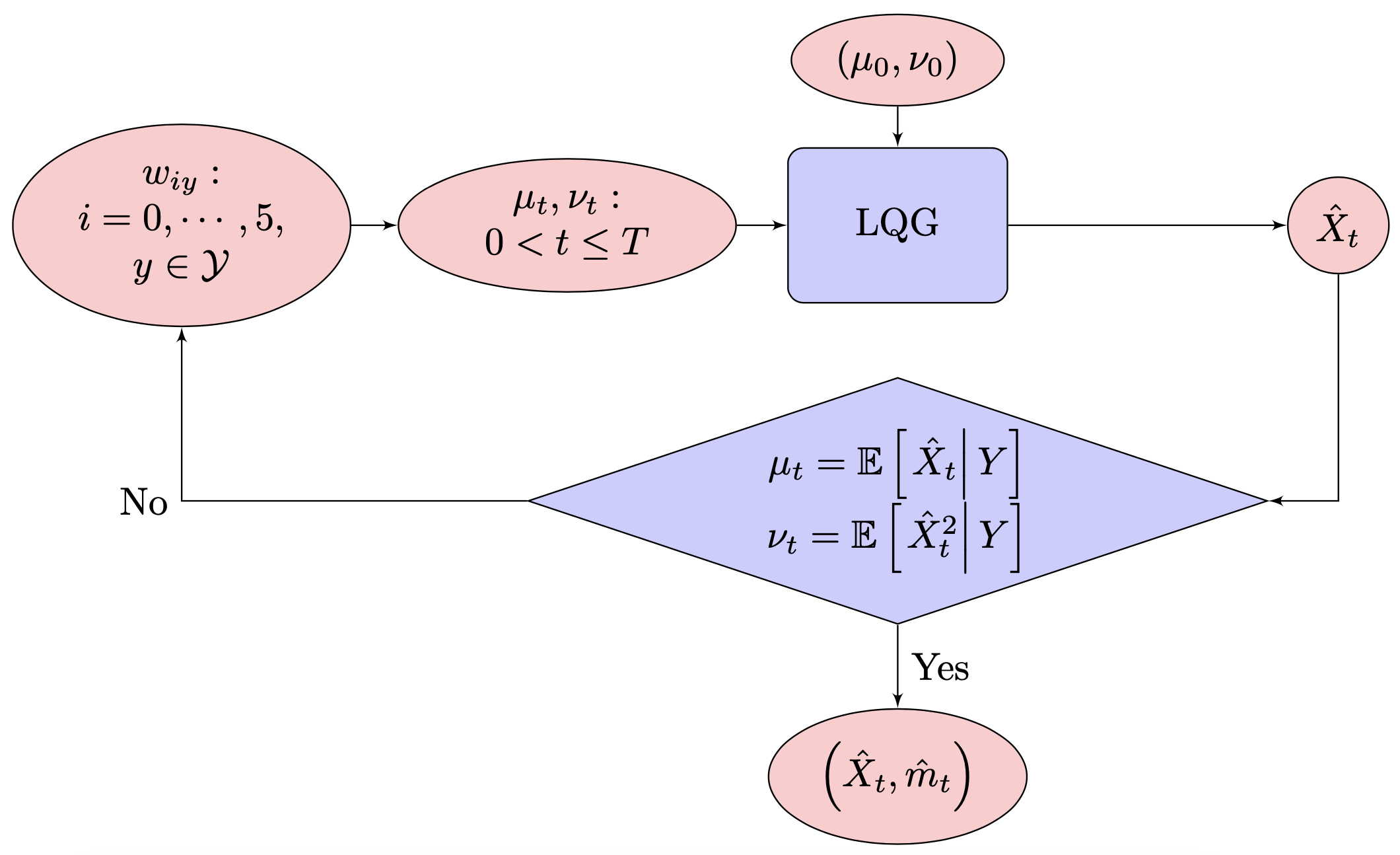
Figure 2. Equivalent MFGs diagram with $\mu_{0}=[m_{0}]_{1}$ and $\nu_{0}=[m_{0}]_{2}$.

The flowchart for our equilibrium is depicted in Figure 2. Subsection 3.2 covers the derivation of the Riccati system for the LQG system with a given population measure flow $m\in\mathcal{M}$, which provides the key building block to MFGs. In Subsection 3.3, we check the fixed point condition and provide a finite-dimensional characterization of MFGs, which gives the first main result Theorem 5.

3.2. The generic player’s control with a given population measure

The advantage of the generic player’s control problem associated with $m\in\mathcal{M}$ is that its optimal path can be characterized via the following classical stochastic control problem:

• (P3) Given smooth functions $w=(w_{i}:i=0,1,\ldots,5)$, find the optimal value $\bar{V}=\bar{V}[w]$

  $$\begin{array}[]{ll}\bar{V}(y,x,t,\bar{\mu},\bar{v})&\displaystyle=\inf_{\alpha\in\mathcal{A}}\mathbb{E}\left[\int_{t}^{T}\left(\frac{1}{2}\alpha_{s}^{2}+\bar{F}(Y_{s},X_{s},\mu_{s},\nu_{s})\right)ds\right.\\ &\displaystyle\hskip 36.135pt\left.+\bar{G}(Y_{T},X_{T},\mu_{T},\nu_{T})\right|Y_{t}=y,X_{t}=x,\mu_{t}=\bar{\mu},\nu_{t}=\bar{\nu}\Big{]}\end{array}$$

  underlying $\mathbb{R}^{4}$-valued processes $(Y,X,\mu,\nu)$ defined through (1)-(3)-(15) with the finite dimensional cost functions: $\bar{F},\bar{G}:\mathbb{R}^{4}\mapsto\mathbb{R}$ given by

  $$\bar{F}(y,x,\bar{\mu},\bar{\nu})=h(y)(x^{2}-2x\bar{\mu}+\bar{\nu}),$$

  $$\bar{G}(y,x,\bar{\mu},\bar{\nu})=g(y)(x^{2}-2x\bar{\mu}+\bar{\nu}),$$

  where $\bar{\mu},\bar{\nu}$ are scalars, while $\mu,\nu$ are used as processes.

Lemma 8.

Given $m\in\mathcal{M}$ associated with $w=(w_{i}:i=0,1,\dots,5)$, the player’s value (4) under assumption (A1) is

$$U[m_{0}](y,x)=\bar{V}(y,x,0,[m_{0}]_{1},[m_{0}]_{2}),$$

and the optimal control has a feedback form

$$\hat{\alpha}_{t}=\bar{\alpha}(Y_{t},X_{t},t,\mu_{t},\nu_{t})$$

underlying the processes $(Y,X,\mu,\nu)$ defined through (1)-(3)-(15), whenever there exists a feedback optimal control $\bar{\alpha}$ for the problem (P3).

Proof.

Due to the quadratic cost structure in (10)-(11), we have enough regularity to all concerned value functions and the details are omitted. ∎

Next, we turn to the solution to the control problem (P3).

3.2.1. HJB equation

For the simplicity of notations, for each $i\in\{0,1,2,3,4,5\}$ and $y\in\mathcal{Y}$, denote the function $(x,t,\bar{\mu},\bar{\nu})\mapsto v(y,x,t,\bar{\mu},\bar{\nu})$ as $v_{y}$, and denote $t\mapsto w_{i}(y,t)$ as $w_{iy}$. We apply similar notations for other functions whenever they have a variable $y\in\mathcal{Y}$. Formally, under enough regularity conditions, the value function $\bar{V}$ defined in (P3) is the solution $v$ of the following coupled HJBs

$$\begin{cases}\displaystyle\partial_{t}v_{y}+\tilde{b}_{1y}x\partial_{x}v_{y}-\frac{1}{2}\left(\tilde{b}_{2y}\partial_{x}v_{y}\right)^{2}+\frac{1}{2}\partial_{xx}v_{y}+\partial_{\mu}v_{y}\left(w_{0y}\bar{\mu}+w_{1y}\right)+\\ \hskip 72.26999pt\displaystyle\partial_{\nu}v_{y}\left(w_{2y}\bar{\mu}+w_{3y}\bar{\nu}+w_{4y}\bar{\mu}^{2}+w_{5y}\right)+\sum_{i=1}^{\kappa}q_{y,i}v_{i}+\bar{F}_{y}=0,\\ \displaystyle v_{y}(x,T,\mu_{T},\nu_{T})=\bar{G}_{y}(x,\mu_{T},\nu_{T}),\ y\in\mathcal{Y}.\end{cases}$$ (16)

Furthermore, the optimal control has to admit the feedback form of

$$\hat{\alpha}(t)=-\tilde{b}_{2}(Y_{t},t)\partial_{x}v({Y_{t}},\hat{X_{t}},t,\mu_{t},\nu_{t}).$$ (17)

Next, we identify what conditions are needed for equating the control problem (P3) and HJB equation. Denote

$$\mathbb{S}=\left\{v\in C^{\infty}:\begin{array}[]{ll}(1+|x|^{2})^{-1}(|v|+|\partial_{t}v|)+\\ \hskip 36.135pt(1+|x|)^{-1}(|\partial_{x}v|+|\partial_{\mu}v|+|\partial_{\nu}v|)+|\partial_{xx}v|<K,\forall(y,x,t,\mu,\nu),\hbox{ for some }K\end{array}\right\}.$$

Lemma 9.

(Verification theorem) Consider the control problem (P3) with some given smooth $w$. Suppose there exists a solution $v\in\mathbb{S}$ of (16). Then, $v_{y}(x,t,\bar{\mu},\bar{\nu})=\bar{V}(y,x,t,\bar{\mu},\bar{\nu})$ holds, and an optimal control is provided by (17).

Proof.

We first prove the verification theorem. Since $v\in\mathbb{S}$, for any admissible $\alpha\in L_{\mathbb{F}}^{4}$, the process $X^{\alpha}$ is well defined and one can use Dynkin’s formula given by Lemma 19 to write

$$\mathbb{E}\left[v(Y_{T},X_{T},T,\mu_{T},\nu_{T})\right]=v(y,x,t,\bar{\mu},\bar{\nu})+\mathbb{E}\left[\int_{t}^{T}\mathcal{G}^{\alpha(s)}v(Y_{s},X_{s},s,\mu_{s},\nu_{s})ds\right],$$

where

$$\mathcal{G}^{a}f(y,x,s,\bar{\mu},\bar{\nu}) =\left(\partial_{t}+\left(\tilde{b}_{1y}x+\tilde{b}_{2y}a\right)\partial_{x}+\frac{1}{2}\partial_{xx}+\mathcal{Q}+\left(w_{0y}\bar{\mu}+w_{1y}\right)\partial_{\bar{\mu}}+\right.$$

$$\quad\quad\quad\left.\left(w_{2y}\bar{\mu}+w_{3y}\bar{\nu}+w_{4y}\bar{\mu}^{2}+w_{5y}\right)\partial_{\bar{\nu}}\right)f(y,x,s,\bar{\mu},\bar{\nu}).$$

Note that HJB actually implies that

$$\inf_{a}\left\{\mathcal{G}^{a}v+\frac{1}{2}a^{2}\right\}=-\bar{F},$$

which again implies

$$-\mathcal{G}^{a}v\leq\frac{1}{2}a^{2}+\bar{F}.$$

Hence, we obtain that for all $\alpha\in L_{\mathbb{F}}^{4}$,

$$\begin{array}[]{ll}\quad v(y,x,t,\bar{\mu},\bar{\nu})\\ \displaystyle=\mathbb{E}\left[\int_{t}^{T}-\mathcal{G}^{\alpha(s)}v(Y_{s},X_{s},s,\mu_{s},\nu_{s})ds\right]+\mathbb{E}\left[v(Y_{T},X_{T},T,\mu_{T},\nu_{T})\right]\\ \displaystyle\leq\mathbb{E}\left[\int_{t}^{T}\left(\frac{1}{2}\alpha^{2}(s)+\bar{F}(Y_{s},X_{s},\mu_{s},\nu_{s})\right)ds\right]+\mathbb{E}\left[\bar{G}(Y_{T},X_{T},\mu_{T},\nu_{T})\right]\\ =J(y,x,t,\alpha,\bar{\mu},\bar{\nu}).\end{array}$$

In the above, if $\alpha$ is replaced by $\hat{\alpha}$ given by the feedback form (17), then since $\partial_{x}v$ is Lipschitz continuous in $x$, there exists corresponding optimal path $\hat{X}\in L_{\mathbb{F}}^{4}$. Thus, $\hat{\alpha}$ is also in $L_{\mathbb{F}}^{4}$. One can repeat all above steps by replacing $X$ and $\alpha$ by $\hat{X}$ and $\hat{\alpha}$, and $\leq$ sign by $=$ sign to conclude that $v$ is indeed the optimal value.

∎

3.2.2. LQG solution

Note that, the costs $\bar{F}$ and $\bar{G}$ of (P3) are quadratic functions in $(x,\bar{\mu},\bar{\nu})$, while the drift function of the process $\nu$ of (15) is not linear in $(x,\bar{\mu},\bar{\nu})$. Therefore, the control problem (P3) does not fall into the standard LQG control framework. Nevertheless, similar to the LQG solution, we guess the value function as a quadratic function in the form of

$$v_{y}(x,t,\bar{\mu},\bar{\nu})= a_{y}(t)x^{2}+d_{y}(t)x+e_{y}(t)\bar{\mu}+f_{y}(t)x\bar{\mu}+k_{y}(t)\bar{\mu}^{2}+b_{y}(t)\bar{\nu}+c_{y}(t),\quad y\in\mathcal{Y}.$$ (18)

With the above setup, for $t\in[0,T]$, the optimal control is

$$\hat{\alpha}_{t}=-\tilde{b}_{2}(Y_{t},t)\partial_{x}v(Y_{t},\hat{X}_{t},t,\mu_{t},\nu_{t})=-\tilde{b}_{2}(Y_{t},t)\left(2a_{Y_{t}}(t)\hat{X}_{t}+d_{Y_{t}}(t)+f_{Y_{t}}(t)\mu_{t}\right),$$ (19)

and the optimal path $\hat{X}$ is

$$d\hat{X}_{t}=\left(\tilde{b}_{1}(Y_{t},t)\hat{X}_{t}-\tilde{b}_{2}^{2}(Y_{t},t)\left(2a_{Y_{t}}(t)\hat{X}_{t}+d_{Y_{t}}(t)+f_{Y_{t}}(t)\mu_{t}\right)\right)dt+dW_{t}.$$ (20)

Denote the following ODE systems for $y\in\mathcal{Y}$,

$$\begin{cases}\displaystyle a_{y}^{\prime}+2\tilde{b}_{1y}a_{y}-2\tilde{b}_{2y}^{2}a_{y}^{2}+\sum_{i=1}^{\kappa}q_{y,i}a_{i}+h_{y}=0,\\ \displaystyle d_{y}^{\prime}+\tilde{b}_{1y}d_{y}-2\tilde{b}_{2y}^{2}a_{y}d_{y}+f_{y}w_{1y}+\sum_{i=1}^{\kappa}q_{y,i}d_{i}=0,\\ \displaystyle e_{y}^{\prime}-\tilde{b}_{2y}^{2}d_{y}f_{y}+2k_{y}w_{1y}+e_{y}w_{0y}+b_{y}w_{2y}+\sum_{i=1}^{\kappa}q_{y,i}e_{i}=0,\\ \displaystyle f_{y}^{\prime}+\tilde{b}_{1y}f_{y}-2\tilde{b}_{2y}^{2}a_{y}f_{y}+f_{y}w_{0y}+\sum_{i=1}^{\kappa}q_{y,i}f_{i}-2h_{y}=0,\\ \displaystyle k_{y}^{\prime}-\frac{1}{2}\tilde{b}_{2y}^{2}f_{y}^{2}+2k_{y}w_{0y}+b_{y}w_{4y}+\sum_{i=1}^{\kappa}q_{y,i}k_{i}=0,\\ \displaystyle b_{y}^{\prime}+b_{y}w_{3y}+\sum_{i=1}^{\kappa}q_{y,i}b_{i}+h_{y}=0,\\ \displaystyle c_{y}^{\prime}+a_{y}-\frac{1}{2}\tilde{b}_{2y}^{2}d_{y}^{2}+e_{y}w_{1y}+b_{y}w_{5y}+\sum_{i=1}^{\kappa}q_{y,i}c_{i}=0,\end{cases}$$ (21)

with terminal conditions

$$a_{y}(T)=g_{y},\ b_{y}(T)=g_{y},\ c_{y}(T)=0,\ d_{y}(T)=0,\ e_{y}(T)=0,\ f_{y}(T)=-2g_{y},\ k_{y}(T)=0.$$ (22)

Lemma 10.

Suppose there exists a unique solution $(a_{y},b_{y},c_{y},d_{y},e_{y},f_{y},k_{y}:y\in\mathcal{Y})$ to the ODE system (21)-(22) on $[0,T]$. Then the value function of (P3) is

$$\bar{V}(y,x,t,\bar{\mu},\bar{\nu})=v_{y}(x,t,\bar{\mu},\bar{\nu})$$ (23)

$$= a_{y}(t)x^{2}+d_{y}(t)x+e_{y}(t)\bar{\mu}+f_{y}(t)x\bar{\mu}+k_{y}(t)\bar{\mu}^{2}+b_{y}(t)\bar{\nu}+c_{y}(t)$$

for $y\in\mathcal{Y}$ and the optimal control and optimal path are given by (19) and (20), respectively.

Proof.

With the form of value function $v_{y}$ given in (18) and the first and second moment of the conditional population density given in (15), we have

$$\partial_{t}v_{y}=a_{y}^{\prime}(t)x^{2}+d_{y}^{\prime}(t)x+e_{y}^{\prime}(t)\bar{\mu}+f_{y}^{\prime}(t)x\bar{\mu}+k_{y}^{\prime}(t)\bar{\mu}^{2}+b_{y}^{\prime}(t)\bar{\nu}+c_{y}^{\prime}(t),$$

$$\partial_{x}v_{y}=2xa_{y}(t)+d_{y}(t)+f_{y}(t)\bar{\mu},$$

$$\partial_{xx}v_{y}=2a_{y}(t),$$

$$\partial_{\bar{\mu}}v_{y}=e_{y}(t)+f_{y}(t)x+2k_{y}(t)\bar{\mu},$$

$$\partial_{\bar{\nu}}v_{y}=b_{y}(t),$$

for $y\in\mathcal{Y}$. Plugging them back to the coupled HJBs in (16), we get a system of ODEs in (21) by equating $x$, $\bar{\mu}$, $\bar{\nu}$-like terms in each equation.

Therefore, any solution $(a_{y},b_{y},c_{y},d_{y},e_{y},f_{y},k_{y}:y\in\mathcal{Y})$ of ODE system (21) leads to the solution of HJB (16) in the form of the quadratic function given by (23). Since the $(a_{y},b_{y},c_{y},d_{y},e_{y},f_{y},k_{y}:y\in\mathcal{Y})$ are differentiable functions on the closed set $[0,T]$, they are also bounded, and the function $v$ meets regularity conditions required by Lemma 9 to conclude the desired result. ∎

3.3. Fixed point condition and the proof of Theorem 5

Going back to the ODE system (21), there are $7\kappa$ equations, while we have total $13\kappa$ deterministic functions of $[0,T]\times\mathbb{R}$ to be determined to characterize MFGs. Those are

$$(a_{y},b_{y},c_{y},d_{y},e_{y},f_{y},k_{y}:y\in\mathcal{Y})\hbox{ and }(w_{iy}:i=0,1,\dots 5,\ y\in\mathcal{Y}).$$

In the following, we identify the missing $6\kappa$ equations by checking the fixed point condition:

$$\mu_{s}=\mathbb{E}\left[\left.\hat{X}_{s}\right|Y\right],\ \nu_{s}=\mathbb{E}\left[\left.\hat{X}_{s}^{2}\right|Y\right],\quad\forall s\in[0,T],$$ (24)

where $\mu$ and $\nu$ are two auxiliary processes $(\mu,\nu)[w]$ defined in (15), see Figure 2. This leads to a complete characterization of the equilibrium for the MFG posed by (P2).

Note that based on the dynamic of the optimal $\hat{X}$ defined in (20), the fixed point condition (24) implies that the first moment $\hat{\mu}_{s}:=\mathbb{E}\left[\left.\hat{X}_{s}\right|Y\right]$ and the second moment $\hat{\nu}_{s}:=\mathbb{E}\left[\left.\hat{X}_{s}^{2}\right|Y\right]$ of the optimal path conditioned on $Y$ satisfy

$$\begin{cases}\displaystyle\hat{\mu}_{s}=\bar{\mu}+\int_{t}^{s}\left(\left(\tilde{b}_{1}(Y_{r},r)-\tilde{b}_{2}^{2}(Y_{r},r)\left(2a_{Y_{r}}(r)+f_{Y_{r}}(r)\right)\right)\hat{\mu}_{r}-\tilde{b}_{2}^{2}(Y_{r},r)d_{Y_{r}}(r)\right)dr,\\ \displaystyle\hat{\nu}_{s}=\bar{\nu}+\int_{t}^{s}\left(1+2\tilde{b}_{1}(Y_{r},r)\hat{\nu}_{r}-\tilde{b}_{2}^{2}(Y_{r},r)\left(4a_{Y_{r}}(r)\hat{\nu}_{r}+2d_{Y_{r}}(r)\hat{\mu}_{r}+2f_{Y_{r}}(r)\hat{\mu}_{r}^{2}\right)\right)dr,\end{cases}$$ (25)

for $s\geq t$. Note that under the optimal control in (19), comparing the terms in (15) and (25), we obtain another $6\kappa$ equations:

$$w_{0y}=\tilde{b}_{1y}-2\tilde{b}_{2y}^{2}a_{y}-\tilde{b}_{2y}^{2}f_{y},\ w_{1y}=-\tilde{b}_{2y}^{2}d_{y},\ w_{2y}=-2\tilde{b}_{2y}^{2}d_{y},$$ (26)

$$w_{3y}=-4\tilde{b}_{2y}^{2}a_{y}+2\tilde{b}_{1y},\ w_{4y}=-2\tilde{b}_{2y}^{2}f_{y},\ w_{5y}=1,$$

for $y\in\mathcal{Y}$. Using further algebraic structures, one can reduce the ODE system of $13\kappa$ equations composed by (21) and (26) into a system of $4\kappa$ equations of the form (12) for the MFG characterization in Theorem 5.

Proof of Theorem 5.

Since $a_{y}$ ($y\in\mathcal{Y}$) has the same expressions as (12), its existence, uniqueness and boundedness are shown in Lemma 23. Given $a_{y}$ ($y\in\mathcal{Y}$) and smooth bounded $w$’s,

$$\left(b_{y},d_{y},e_{y},f_{y}:y\in\mathcal{Y}\right)$$

is a coupled linear system, and their existence, uniqueness and boundedness is shown by Theorem 12.1 in [2]. Similarly, given $(b_{y},d_{y},f_{y}:y\in\mathcal{Y}$), $(k_{y},c_{y}:y\in\mathcal{Y}$) is a linear system, and their existence and uniqueness is also guaranteed by Theorem 12.1 in [2].

The ODE system (21) can be rewritten by

$$\begin{cases}\displaystyle a_{y}^{\prime}+2\tilde{b}_{1y}a_{y}-2\tilde{b}_{2y}^{2}a_{y}^{2}+\sum_{i=1}^{\kappa}q_{y,i}a_{i}+h_{y}=0,\\ \displaystyle d_{y}^{\prime}+\tilde{b}_{1y}d_{y}-2\tilde{b}_{2y}^{2}a_{y}d_{y}-\tilde{b}_{2y}^{2}f_{y}d_{y}+\sum_{i=1}^{\kappa}q_{y,i}d_{i}=0,\\ \displaystyle e_{y}^{\prime}-\tilde{b}_{2y}^{2}d_{y}f_{y}-2\tilde{b}_{2y}^{2}k_{y}d_{y}+e_{y}\left(\tilde{b}_{1y}-2\tilde{b}_{2y}^{2}a_{y}-\tilde{b}_{2y}^{2}f_{y}\right)-2\tilde{b}_{2y}^{2}b_{y}d_{y}+\sum_{i=1}^{\kappa}q_{y,i}e_{i}=0,\\ \displaystyle f_{y}^{\prime}+\tilde{b}_{1y}f_{y}-2\tilde{b}_{2y}^{2}a_{y}f_{y}+f_{y}\left(\tilde{b}_{1y}-2\tilde{b}_{2y}^{2}a_{y}-\tilde{b}_{2y}^{2}f_{y}\right)+\sum_{i=1}^{\kappa}q_{y,i}f_{i}-2h_{y}=0,\\ \displaystyle k_{y}^{\prime}-\frac{1}{2}\tilde{b}_{2y}^{2}f_{y}^{2}+2k_{y}\left(\tilde{b}_{1y}-2\tilde{b}_{2y}^{2}a_{y}-\tilde{b}_{2y}^{2}f_{y}\right)-2\tilde{b}_{2y}^{2}b_{y}f_{y}+\sum_{i=1}^{\kappa}q_{y,i}k_{i}=0,\\ \displaystyle b_{y}^{\prime}+b_{y}\left(-4\tilde{b}_{2y}^{2}a_{y}+2\tilde{b}_{1y}\right)+\sum_{i=1}^{\kappa}q_{y,i}b_{i}+h_{y}=0,\\ \displaystyle c_{y}^{\prime}+a_{y}-\frac{1}{2}\tilde{b}_{2y}^{2}d_{y}^{2}-2\tilde{b}_{2y}^{2}d_{y}e_{y}+b_{y}+\sum_{i=1}^{\kappa}q_{y,i}c_{i}=0,\end{cases}$$

with the terminal conditions

$$a_{y}(T)=g_{y},\ b_{y}(T)=g_{y},\ c_{y}(T)=0,\ d_{y}(T)=0,\ e_{y}(T)=0,\ f_{y}(T)=-2g_{y},\ k_{y}(T)=0.$$

Since $a_{y},b_{y}$ ($y\in\mathcal{Y}$) has the same expressions as (12), its existence, uniqueness and boundedness are shown in Lemma 23. Meanwhile, with the given $(a_{y},b_{y}:y\in\mathcal{Y})$, we denote $l_{y}=2a_{y}+f_{y}$, and then

$$l_{y}^{\prime}+2\tilde{b}_{1y}l_{y}-\tilde{b}_{2y}^{2}l_{y}^{2}+\sum_{i=1}^{\kappa}q_{y,i}l_{i}=0\text{ , }l_{y}(T)=0.$$

By Lemma 21 and Lemma 22 in Appendix, there exists a unique solution for $l_{y}\ (y\in\mathcal{Y})$, which is $l_{y}=0,y\in\mathcal{Y}$. This gives $f_{y}=-2a_{y}$ and $d_{y}^{\prime}+\tilde{b}_{1y}d_{y}+\sum_{i=1}^{\kappa}q_{y,i}d_{i}=0$, which implies $d_{y}=0,y\in\mathcal{Y}$. Then, the equation for $e_{y}$ can be simplified as $e_{y}^{\prime}+\tilde{b}_{1y}e_{y}+\sum_{i=1}^{\kappa}q_{y,i}e_{i}=0$, which indicates that $e_{y}=0,y\in\mathcal{Y}$. For $k_{y},c_{y}$, with the given of $(a_{y},b_{y}:y\in\mathcal{Y})$, we have

$$k_{y}^{\prime}+2\tilde{b}_{1y}k_{y}-2\tilde{b}_{2y}^{2}a_{y}^{2}+4\tilde{b}_{2y}^{2}a_{y}b_{y}+\sum_{i=1}^{\kappa}q_{y,i}k_{i}=0\text{ , }k_{y}(T)=0,$$

$$c_{y}^{\prime}+a_{y}+b_{y}+\sum_{i=1}^{\kappa}q_{y,i}c_{i}=0\text{ , }c_{y}(T)=0.$$

The existence and uniqueness of the solution for $k_{y},c_{y}\ (y\in\mathcal{Y})$ are yielded by Theorem 12.1 in [2].

Note that in this case, since $2a_{y}+f_{y}=0$ and $d_{y}=0$ for $y\in\mathcal{Y}$, from (25) we have

$$\hat{\mu}_{s}=\bar{\mu}+\int_{t}^{s}\tilde{b}_{1}(Y_{r},r)\hat{\mu}_{r}\ dr$$

for all $s\in[t,T]$. Then

$$\hat{\nu}_{s}=\bar{\nu}+\int_{t}^{s}\left(1+2\tilde{b}_{1}(Y_{r},r)\hat{\nu}_{r}-4\tilde{b}_{2}^{2}(Y_{r},r)a_{Y_{r}}(r)\hat{\nu}_{r}+4\tilde{b}_{2}^{2}(Y_{r},r)a_{Y_{r}}(r)\hat{\mu}_{r}^{2}\right)\,dr.$$

Plugging $d_{y}=0$ for $y\in\mathcal{Y}$ back to (19), we obtain the optimal control by

$$\hat{\alpha}_{s}=-2\tilde{b}_{2}^{2}(Y_{s},s)a_{Y_{s}}(s)\left(\hat{X}_{s}-\hat{\mu}_{s}\right).$$

Since we have $d_{y}=0$ for $y\in\mathcal{Y}$, the value function can be simplified from (18) to

$$v_{y}(x,t,\bar{\mu},\bar{\nu})=a_{y}(t)x^{2}{-2a_{y}(t)x\bar{\mu}+k_{y}(t)\bar{\mu}^{2}}+b_{y}(t)\bar{\nu}+c_{y}(t).$$

By the equivalence Lemma 8, it yields the value function $U$ of Theorem 5 . Moreover, since $f_{y}=-2a_{y}$ and $k_{y}\neq 0$, the ODE system (21) together with (26) can be reduced into (12). From the Lemma 23, the existence and uniqueness of $(a_{y},b_{y},c_{y},k_{y}:y\in\mathcal{Y})$ in (12) is guaranteed.

∎

4. The $N$-Player Game and its Convergence to MFGs

In this section, we show the convergence of the $N$-player game to MFGs. To simplify the presentation, we may omit the superscript $(N)$ for the processes in the probability space $\Omega^{(N)}$, whenever there is no confusion. First, we solve the $N$-player game in Subsection 4.1, which provides a Riccati system consisting of $O(N^{3})$ equations. Subsection 4.2 reduces the corresponding Riccati system into an ODE system whose dimension is independent of $N$. This becomes the key building block of the convergence rate obtained in Subsection 4.3. To obtain the convergence rate, Subsection 4.3 provides an explicit embedding of some processes in $\Omega^{(N)}$ into the probability space $\Omega$. Note that, $\Omega^{(N)}$ is much richer than $\Omega$ since $\Omega^{(N)}$ contains $N$ Brownian motions while $\Omega$ has only two Brownian motions. Therefore, careful treatment has to be carried out to some processes of our interest, otherwise, such an embedding is in general implausible.

4.1. Characterization of the $N$-player game by Riccati system

The $N$-player game is indeed an $N$-coupled stochastic LQG problem by its very own definition, see Subsection 2.3. Therefore, the solution can be derived via Riccati system with the existing LQG theory given below: For $i=1,2,\ldots,N$, $y\in\mathcal{Y}$,

$$\begin{cases}\displaystyle A_{iy}^{\prime}+2\tilde{b}_{1y}e_{i}e_{i}^{\top}A_{iy}-2\tilde{b}_{2y}^{2}A_{iy}^{\top}e_{i}e_{i}^{\top}A_{iy}+\sum_{j\neq i}^{N}\left(2\tilde{b}_{1y}e_{j}e_{j}^{\top}A_{iy}-4\tilde{b}_{2y}^{2}A_{jy}^{\top}e_{j}e_{j}^{\top}A_{iy}\right)\\ \displaystyle\hskip 108.405pt+\sum_{j=1}^{\kappa}q_{y,j}A_{ij}+\frac{h_{y}}{N}\sum_{j\neq i}^{N}\left(e_{i}-e_{j}\right)\left(e_{i}-e_{j}\right)^{\top}=0,\\ \displaystyle B_{iy}^{\prime}+\sum_{j\neq i}^{N}\left(\tilde{b}_{1y}e_{j}e_{j}^{\top}B_{iy}-2\tilde{b}_{2y}^{2}A_{iy}^{\top}e_{j}e_{j}^{\top}B_{jy}-2\tilde{b}_{2y}^{2}A_{jy}^{\top}e_{j}e_{j}^{\top}B_{iy}\right)\\ \displaystyle\hskip 108.405pt+\tilde{b}_{1y}e_{i}e_{i}^{\top}B_{iy}-2\tilde{b}_{2y}^{2}A_{iy}^{\top}e_{i}e_{i}^{\top}B_{iy}+\sum_{j=1}^{\kappa}q_{y,j}B_{ij}=0,\\ \displaystyle C_{iy}^{\prime}-\frac{1}{2}\tilde{b}_{2y}^{2}B_{iy}^{\top}e_{i}e_{i}^{\top}B_{iy}-\sum_{j\neq i}^{N}\tilde{b}_{2y}^{2}B_{jy}^{\top}e_{j}e_{j}^{\top}B_{iy}+\sum_{j=1}^{N}tr(A_{jy})+\sum_{j=1}^{\kappa}q_{y,j}C_{ij}=0,\\ \displaystyle A_{iy}(T)=\frac{g_{y}}{N}\Lambda_{i},\ B_{iy}(T)=0\cdot\mathds{1}_{N},\ C_{iy}(T)=0,\end{cases}$$ (27)

where the solutions consist of $N\times N$ symmetric matrices $A_{iy}$’s, $N$-dimensional vectors $B_{iy}$’s, and $C_{iy}\in\mathbb{R}$. In the above, $\mathds{1}_{N}$ is the $N$-dimensional vector with all entries are $1$, $\Lambda_{i}$’s are $N\times N$ matrices with diagonal $1$ except $(\Lambda_{i})_{ii}=N-1$, $\left(\Lambda_{i}\right)_{ij}=\left(\Lambda_{i}\right)_{ji}=-1$ for any $j\neq i$ and the rest entries as 0, and $e_{i}$’s are the $N$-dimensional natural basis.

Lemma 11.

Suppose $(A_{iy},B_{iy},C_{iy}:i=1,2,\ldots,N,\ y\in\mathcal{Y})$ is the solution of (27). Then, the value functions of $N$-player game defined by (9) are

$$V_{i}(y,x^{(N)})=(x^{(N)})^{\top}A_{iy}(0)x^{(N)}+(x^{(N)})^{\top}B_{iy}(0)+C_{iy}(0),\quad i=1,2,\dots,N.$$

Moreover, the path and the control under the equilibrium are

$$d\hat{X}_{it}=\left(\tilde{b}_{1}(Y_{t},t)\hat{X}_{it}-\tilde{b}_{2}^{2}(Y_{t},t)\left(2(A_{iY_{t}})_{i}^{\top}\hat{X}_{t}+(B_{iY_{t}})_{i}\right)\right)dt+dW_{it},\quad i=1,2,\dots,N,$$ (28)

and

$$\hat{\alpha}_{it}=-\tilde{b}_{2}(Y_{t},t)\left(2(A_{iY_{t}})_{i}^{\top}\hat{X}_{t}+(B_{iY_{t}})_{i}\right),$$

where $(A)_{i}$ denotes the $i$-th column of matrix $A$, $(B)_{i}$ denotes the $i$-th entry of vector $B$ and $\hat{X}_{t}=[\hat{X}_{1t},\hat{X}_{2t},\dots,\hat{X}_{Nt}]^{\top}$.

Proof.

It is standard that, under enough regularities, the value function $V(y,x^{(N)})=(V_{1},V_{2},\dots,V_{N})(y,x^{(N)})$ of the $N$-player game can be lifted to the solution $v_{iy}(x^{(N)},t)$ of the following system of HJB equations, for $i=1,2,\ldots,N$ and $y\in\mathcal{Y}$,

$$\begin{cases}\displaystyle\partial_{t}v_{iy}+\tilde{b}_{1y}x_{i}\partial_{i}v_{iy}-\frac{1}{2}\left(\tilde{b}_{2y}\partial_{i}v_{iy}\right)^{2}+\sum_{j\neq i}^{N}\left(\tilde{b}_{1y}x_{j}-\tilde{b}_{2y}^{2}\partial_{j}v_{jy}\right)\partial_{j}v_{iy}\\ \displaystyle\hskip 108.405pt+\frac{1}{2}\Delta v_{iy}+\sum_{j=1}^{\kappa}q_{y,j}v_{ij}+\frac{h_{y}}{N}\sum_{j\neq i}^{N}\left(\left(e_{i}-e_{j}\right)^{\top}x^{(N)}\right)^{2}=0,\\ \displaystyle v_{iy}(x^{(N)},T)=\frac{g_{y}}{N}\sum_{j\neq i}^{N}\left((e_{i}-e_{j})^{\top}x^{(N)}\right)^{2}.\end{cases}$$ (29)

Then, the value functions $V$ of $N$-player game defined by (9) is $V_{i}(y,x^{(N)})=v_{iy}(x^{(N)},0)$ for all $i=1,2,\dots,N$. Moreover, the path and the control under the equilibrium are

$$d\hat{X}_{it}=\left(\tilde{b}_{1}(Y_{t},t)\hat{X}_{it}-\tilde{b}_{2}^{2}(Y_{t},t)\partial_{i}v_{iY_{t}}(\hat{X}_{t},t)\right)dt+dW_{it},\quad i=1,2,\dots,N,$$

and

$$\hat{\alpha}_{it}=-\tilde{b}_{2}(Y_{t},t)\partial_{i}v_{iY_{t}}(\hat{X}_{t},t).$$

The proof is the application of Dynkin’s formula and the details are omitted here. Due to its LQG structure, the value function leads to a quadratic function of the form

$$v_{iy}(x^{(N)},t)=(x^{(N)})^{\top}A_{iy}(t)x^{(N)}+(x^{(N)})^{\top}B_{iy}(t)+C_{iy}(t).$$

For each $i=1,2,\dots,N$, after plugging $V_{iy}$ into (29), and matching the coefficient of variables, we get the desired results. ∎

4.2. Reduced Riccati form for the equilibrium

So far, the $N$-player game and MFG have been characterized by Lemma 11 and Theorem 5, respectively. One of our main objectives is to investigate the convergence of the generic optimal path $\hat{X}_{1t}^{(N)}$ of $N$-player game generated (27)-(28) to the optimal path $\hat{X}_{t}$ of MFG generated by (12)-(13).

Note that $\hat{X}_{t}$ relies only on $\kappa$ functions $(a_{y}:y\in\mathcal{Y})$ from the simple ODE system (12) while $\rho(\hat{X}_{t}^{(N)})$ depends on $O(N^{3})$ functions from $(A_{iy}:i=1,2,\ldots,N,\ y\in\mathcal{Y})$ solved from a huge Riccati system (27). Therefore, it is almost a hopeless task for a meaningful comparison between these two processes without gaining further insight into the complex structure of the Riccati system (27).

To proceed, let us first observe some hidden patterns from a numerical result for the solution of Riccati (27). The following matrix shows $A_{20}$ at $t=1$ for $N=5$ with the same parameters as in Figure 3 and Figure 4 in Section 5.1:

$$A_{20}(1)=\begin{bmatrix}0.1319&-0.1924&0.0202&0.0202&0.0202\\ -0.1924&0.7696&-0.1924&-0.1924&-0.1924\\ 0.0202&-0.1924&0.1319&0.0202&0.0202\\ 0.0202&-0.1924&0.0202&0.1319&0.0202\\ 0.0202&-0.1924&0.0202&0.0202&0.1319\end{bmatrix}.$$

Interestingly enough, we observe that the entire 25 entries of $A_{20}(1)$ indeed consists of $4$ distinct values. Moreover, similar computation with different values of $N$ only yields a larger table depending on $N$, but always consists of $4$ values. Inspired by this accidental discovery from the above numerical example, we may want to believe and prove a pattern of the matrix $A_{iy}$ in the following form:

$$(A_{iy})_{pq}=\begin{cases}a_{1y}(t),&\text{ if }p=q=i,\\ a_{2y}(t),&\text{ if }p=q\neq i,\\ a_{3y}(t),&\text{ if }p\neq q,p=i\text{ or }q=i,\\ a_{4y}(t),&\text{ otherwise},\end{cases}$$ (30)

for $y\in\mathcal{Y}$. The next result justifies the above pattern: the $N^{2}$ entries of the matrix $A_{iy}$ can be embedded to a $2\kappa$-dimensional vector space no matter how big $N$ is.

Lemma 12.

There exists a unique solution $(a_{1y}^{N},a_{2y}^{N})$ from the ODE system(31)

$$\begin{cases}\displaystyle a_{1y}^{\prime}+2\tilde{b}_{1y}a_{1y}-\frac{2(N+1)}{N-1}\tilde{b}_{2y}^{2}a_{1y}^{2}+\sum_{j=1}^{\kappa}q_{y,j}a_{1j}+\frac{N-1}{N}h_{y}=0,\\ \displaystyle a_{2y}^{\prime}+2\tilde{b}_{1y}a_{2y}+\frac{2}{(N-1)^{2}}\tilde{b}_{2y}^{2}a_{1y}^{2}-\frac{4N}{N-1}\tilde{b}_{2y}^{2}a_{1y}a_{2y}+\sum_{j=1}^{\kappa}q_{y,j}a_{2j}+\frac{h_{y}}{N}=0,\\ \displaystyle a_{1y}(T)=\frac{N-1}{N}g_{y},\ a_{2y}(T)=\frac{g_{y}}{N},\end{cases}$$ (31)

for $y\in\mathcal{Y}$. Moreover, the path and the control of player $i$ under the equilibrium are

$$d\hat{X}_{it}^{(N)}=\left(\tilde{b}_{1}(Y_{t}^{(N)},t)\hat{X}_{it}^{(N)}-2\tilde{b}_{2}^{2}(Y_{t}^{(N)},t)a_{1Y_{t}^{(N)}}^{N}(t)\left(\hat{X}_{it}^{(N)}-\frac{1}{N-1}\sum_{j\neq i}^{N}\hat{X}_{jt}^{(N)}\right)\right)dt+dW_{it}^{(N)},$$ (32)

and

$$\hat{\alpha}_{it}^{(N)}=-2\tilde{b}_{2}(Y_{t}^{(N)},t)a_{1Y_{t}^{(N)}}^{N}(t)\left(\hat{X}_{it}^{(N)}-\frac{1}{N-1}\sum_{j\neq i}^{N}\hat{X}_{jt}^{(N)}\right)$$

for $i=1,2,\dots,N$.

Proof.

It is obvious to see that in the Riccati system (27), $B_{iy}=0$ for all $i=1,2,\dots,N$ and $y\in\mathcal{Y}$. Note that in this case, for $i=1,2,\dots,N$, the optimal control is given by

$$\hat{\alpha}_{i}^{(N)}=-2\tilde{b}_{2}(Y_{t}^{(N)},t)\sum_{j=1}^{N}(A_{iY_{t}^{(N)}})_{ij}\hat{X}_{jt}^{(N)}=-2\tilde{b}_{2}(Y_{t}^{(N)},t)\left(A_{iY_{t}^{(N)}}\right)_{i}^{\top}\hat{X}^{(N)}_{t}.$$

Plugging the pattern (30) into the differential equation of $A_{iy}$, we have

$$a_{1y}^{\prime}+2\tilde{b}_{1y}a_{1y}-2\tilde{b}_{2y}^{2}a_{1y}^{2}-4(N-1)\tilde{b}_{2y}^{2}a_{3y}^{2}+\sum_{j=1}^{\kappa}q_{y,j}a_{1j}+\frac{N-1}{N}h_{y}=0,$$

$$a_{2y}^{\prime}+2\tilde{b}_{1y}a_{2y}-2\tilde{b}_{2y}^{2}a_{3y}^{2}-4\tilde{b}_{2y}^{2}\left(a_{1y}a_{2y}+(N-2)a_{3y}a_{4y}\right)+\sum_{j=1}^{\kappa}q_{y,j}a_{2j}+\frac{h_{y}}{N}=0,$$

$$a_{3y}^{\prime}+2\tilde{b}_{1y}a_{3y}-2\tilde{b}_{2y}^{2}a_{1y}a_{3y}-4\tilde{b}_{2y}^{2}\left(a_{1y}a_{3y}+(N-2)a_{3y}^{2}\right)+\sum_{j=1}^{\kappa}q_{y,j}a_{3j}-\frac{h_{y}}{N}=0,$$

$$a_{3y}^{\prime}+2\tilde{b}_{1y}a_{3y}-2\tilde{b}_{2y}^{2}a_{1y}a_{3y}-4\tilde{b}_{2y}^{2}\left(a_{2y}a_{3y}+(N-2)a_{3y}a_{4y}\right)+\sum_{j=1}^{\kappa}q_{y,j}a_{3j}-\frac{h_{y}}{N}=0,$$

$$a_{4y}^{\prime}+2\tilde{b}_{1y}a_{4y}-2\tilde{b}_{2y}^{2}a_{3y}^{2}-4\tilde{b}_{2y}^{2}\left(a_{2y}a_{3y}+a_{1y}a_{4y}+(N-3)a_{3y}a_{4y}\right)+\sum_{j=1}^{\kappa}q_{y,j}a_{4j}=0,$$

which gives $a_{1y}+(N-2)a_{3y}=a_{2y}+(N-2)a_{4y}$ since two expressions for $a_{3y}$ should be identical. This implies that $\left(a_{1y}+(N-2)a_{3y}\right)^{\prime}=\left(a_{2y}+(N-2)a_{4y}\right)^{\prime}$ or

$$-2\tilde{b}_{1y}a_{1y}+2\tilde{b}_{2y}^{2}a_{1y}^{2}+4(N-1)\tilde{b}_{2y}^{2}a_{3y}^{2}-\frac{N-1}{N}h_{y}-\sum_{j=1}^{\kappa}q_{y,j}a_{1j}$$

$$+(N-2)\left(-2\tilde{b}_{1y}a_{3y}+2\tilde{b}_{2y}^{2}a_{1y}a_{3y}+4\tilde{b}_{2y}^{2}\left(a_{2y}a_{3y}+(N-2)a_{3y}a_{4y}\right)-\sum_{j=1}^{\kappa}q_{y,j}a_{3j}+\frac{h_{y}}{N}\right)$$

$$= -2\tilde{b}_{1y}a_{2y}+2\tilde{b}_{2y}^{2}a_{3y}^{2}+4\tilde{b}_{2y}^{2}\left(a_{1y}a_{2y}+(N-2)a_{3y}a_{4y}\right)-\sum_{j=1}^{\kappa}q_{y,j}a_{2j}-\frac{h_{y}}{N}$$

$$+(N-2)\left(-2\tilde{b}_{1y}a_{4y}+2\tilde{b}_{2y}^{2}a_{3y}^{2}+4\tilde{b}_{2y}^{2}\left(a_{1y}a_{4y}+a_{2y}a_{3y}+(N-3)a_{3y}a_{4y}\right)-\sum_{j=1}^{\kappa}q_{y,j}a_{4j}\right).$$

After combining terms and substituting $a_{2y}+(N-2)a_{4y}$ with $a_{1y}+(N-2)a_{3y}$, we get $a_{1y}^{2}+(N-2)a_{1y}a_{3y}-(N-1)a_{3y}^{2}=0$, which yields $a_{3y}=a_{1y}$ or $a_{3y}=-\frac{1}{N-1}a_{1y}$. Note that $a_{3y}\neq a_{1y}$ due to their different differential equations. Hence, we can conclude that $a_{3y}=-\frac{1}{N-1}a_{1y}$. In conclusion, for $i=1,2,\dots,N$, $A_{iy}$ ($y\in\mathcal{Y}$) has the following expressions:

$$(A_{iy})_{pq}=\begin{cases}a_{1y}(t),&\text{ if }p=q=i,\\ a_{2y}(t),&\text{ if }p=q\neq i,\\ -\frac{1}{N-1}a_{1y}(t),&\text{ if }p\neq q,p=i\text{ or }q=i,\\ \frac{1}{(N-1)(N-2)}a_{1y}(t)-\frac{1}{N-2}a_{2y}(t),&\text{ otherwise}.\end{cases}$$

The existence and uniqueness of (27) is equivalent to the existence and uniqueness of (31). For $a_{1y}$, the existence and uniqueness can be deduced from Lemma 21 and 22. Given $a_{1y}$’s, $a_{2y}$’s are linear equations, thus their existence and uniqueness are guaranteed by Theorem 12.1 in [2]. Together with previous discussions, we conclude the results. ∎

4.3. Convergence

Based on the current progress, let us reiterate our goal (P1) for the convergence. Our objective is the convergence of the joint distribution $\mathcal{L}(\hat{X}_{1t}^{(N)},Y_{t}^{(N)})$ of $N$-player game generated (31)-(32) in the probability space $\Omega^{(N)}$ to the distribution $\mathcal{L}(\hat{X}_{t},Y_{t})$ of MFG generated by (12)-(13) in the probability space $\Omega$. More precisely, we want to find a number $\eta>0$ satisfying

$$\mathbb{W}_{2}\left(\mathcal{L}(\hat{X}_{1t}^{(N)},Y_{t}^{(N)}),\mathcal{L}(\hat{X}_{t},Y_{t})\right)=O\left(N^{-\eta}\right),$$ (33)

where $\mathbb{W}_{2}$ is the 2-Wasserstein metric. This procedure is given in the following two steps:

1. We will construct a process $Z^{N}$ in the probability space $\Omega$, who provides exact copy of the joint distribution in the sense of

   $$\mathcal{L}(\hat{X}_{1t}^{(N)},Y_{t}^{(N)})=\mathcal{L}(Z^{N},Y).$$

   Note that, the (32) shows that $\hat{X}_{1t}^{(N)}$ correlates to $N$ many Brownian motions $\{W_{i}^{(N)}:i=1,2,\ldots,N\}$ from a much richer space $\Omega^{(N)}$ while $\Omega$ is a much smaller space having only two Brownian motions $W$ and $B$. Therefore, such an embedding essentially requires to represent $\hat{X}_{1t}^{(N)}$ by two independent Brownian motions and is in general not possible. However, due to the symmetric structure of MFG (or the nature of the mean field effect), the embedding is possible and the details are provided in Lemma 13.

2. By Proposition 1, we can use distribution copy $(Z^{N},Y)$ in $\Omega$ to write

   $$\mathbb{W}_{2}^{2}\left(\mathcal{L}(\hat{X}_{1t}^{(N)},Y_{t}^{(N)}),\mathcal{L}(\hat{X}_{t},Y_{t})\right)\leq\mathbb{E}\left[\left|Z_{t}^{N}-\hat{X}_{t}\right|^{2}\right].$$ (34)

   To obtain the estimate of the above right hand side, we shall compare the (35) of $Z^{N}$ and (13) of $\hat{X}$, and it becomes essential to obtain the convergence rate of the ODE system (31) towards the ODE system (12). The details are provided in Lemma 14.

Lemma 13.

Let $\{X_{0}^{i}:i\in\mathbb{N}\}$ be i.i.d. random variables in $\Omega$ independent to $(W,B,Y)$ with $X_{0}^{1}=X_{0}$. Let $Z^{N}$ be the solution of

$$Z_{t}^{N}=X_{0}+\int_{0}^{t}\tilde{b}_{1}(Y_{s},s)Z_{s}^{N}ds-\int_{0}^{t}2\tilde{b}_{2}^{2}(Y_{s},s)\hat{a}_{1Y_{s}}^{N}(s)\left(Z_{s}^{N}-\bar{X}_{s}^{N}\right)ds+W_{t},$$ (35)

where

$$d\bar{X}_{t}^{N}=\tilde{b}_{1}(Y_{t},t)\bar{X}_{t}^{N}dt+\frac{\sqrt{N-1}}{N}dB_{t}+\frac{1}{N}dW_{t},\quad\bar{X}_{0}^{N}=\frac{1}{N}\sum_{i=1}^{N}X_{0}^{i},$$

and

$$\hat{a}_{1y}^{N}=\frac{N}{N-1}a_{1y}^{N},$$

where $a_{1y}^{N}$ is from the ODE system(31). Then, $(Z^{N}_{t},Y_{t})$ in $(\Omega,\mathcal{F}_{T},\mathbb{P})$ has the same distribution as $(\hat{X}_{1t}^{(N)},Y_{t}^{(N)})$ in $(\Omega^{(N)},\mathcal{F}_{T}^{(N)},\mathbb{P}^{(N)})$.

Proof.

Continued from the Lemma 12, player $i$’s path in the $N$-player game follows

$$\hat{X}_{it}^{(N)}=x_{i}^{(N)}+\int_{0}^{t}\tilde{b}_{1}(Y_{s}^{(N)},s)\hat{X}_{is}^{(N)}ds-\int_{0}^{t}2\tilde{b}_{2}^{2}(Y_{s}^{(N)},s)a_{1Y_{s}^{(N)}}^{N}(s)\left(\hat{X}_{is}^{(N)}-\frac{1}{N-1}\sum_{j\neq i}^{N}\hat{X}_{js}^{(N)}\right)ds+W_{it}^{(N)}.$$

With the notation

$$\bar{X}^{(N)}_{s}=\frac{1}{N}\sum_{i=1}^{N}\hat{X}_{is}^{(N)},$$

one can rewrite the path by

$$\hat{X}_{it}^{(N)}=x_{i}^{(N)}+\int_{0}^{t}\tilde{b}_{1}(Y_{s}^{(N)},s)\hat{X}_{is}^{(N)}ds-\int_{0}^{t}2\tilde{b}_{2}^{2}(Y_{s}^{(N)},s)\hat{a}_{1Y_{s}^{(N)}}^{N}(s)\left(\hat{X}_{is}^{(N)}-\bar{X}_{s}^{(N)}\right)ds+W_{it}^{(N)}.$$ (36)

By adding up the above equations (36) indexed by $i=1$ to $N$, one can have

$$\bar{X}^{(N)}_{t} =\bar{x}^{(N)}+\int_{0}^{t}\tilde{b}_{1}(Y_{s}^{(N)},s)\bar{X}_{s}^{(N)}ds+\frac{1}{N}\sum_{i=1}^{N}W_{it}^{(N)}$$ (37)

$$=\bar{x}^{(N)}+\int_{0}^{t}\tilde{b}_{1}(Y_{s}^{(N)},s)\bar{X}_{s}^{(N)}ds+\frac{\sqrt{N-1}}{N}\left(\sqrt{N-1}\bar{W}_{-it}^{(N)}\right)+\frac{1}{N}W_{it}^{(N)},$$

where $\bar{W}_{-it}^{(N)}:=\frac{1}{N-1}\sum_{j\neq i}W_{jt}^{(N)}$.

Next, we define solution maps of (36) and (37):

$$\bar{G}_{t}(x,\phi,W_{1},W_{2})=\mathcal{E}_{t}(\phi)\left(x+\int_{0}^{t}\mathcal{E}_{s}(-\phi)d(W_{1s}+W_{2s})\right)$$ (38)

and

$$G_{t}(x,\phi_{1},\phi_{2},\phi_{3},W)=x\mathcal{E}_{t}(\phi_{1}-\phi_{2})+\mathcal{E}_{t}(\phi_{1}-\phi_{2})\int_{0}^{t}\mathcal{E}_{s}(-\phi_{1}+\phi_{2})\left(\phi_{2}(s)\phi_{3}(s)ds+dW_{s}\right),$$ (39)

where

$$\mathcal{E}_{t}(\phi)=\exp\left\{\int_{0}^{t}\phi_{s}ds\right\}.$$

Now, we can rewrite $\bar{X}_{t}^{(N)}$ of (37) and $\hat{X}_{1t}^{(N)}$ of (36) as

$$\bar{X}_{t}^{(N)}=\bar{G}_{t}\left(\frac{1}{N}\sum_{i=1}^{N}x_{i}^{(N)},\tilde{b}_{1}(Y_{.}^{(N)},\cdot),\frac{\sqrt{N-1}}{N}\left(\sqrt{N-1}\bar{W}_{-1}^{(N)}\right),\frac{1}{N}W_{1}^{(N)}\right),$$

and

$$\hat{X}_{1t}^{(N)}=G_{t}\left(x_{1}^{(N)},\tilde{b}_{1}(Y^{(N)}_{\cdot},\cdot),2\tilde{b}_{2}(Y^{(N)}_{\cdot},\cdot)\hat{a}^{N}_{1}(Y^{(N)}_{\cdot},\cdot),\bar{X}^{(N)}(\cdot),W_{1}^{(N)}\right)$$

Meanwhile, $(Z^{N},\bar{X}^{N})$ of (35) can also be written in the form of

$$\bar{X}_{t}^{N}=\bar{G}_{t}\left(\frac{1}{N}\sum_{i=1}^{N}X_{0}^{i},\tilde{b}_{1}(Y_{.},\cdot),\frac{\sqrt{N-1}}{N}B,\frac{1}{N}W\right),$$

and

$$Z_{t}^{N}=G_{t}\left(X_{0},\tilde{b}_{1}(Y_{\cdot},\cdot),2\tilde{b}_{2}(Y_{\cdot},\cdot)\hat{a}^{N}_{1}(Y_{\cdot},\cdot),\bar{X}^{N}(\cdot),W\right)$$ (40)

Finally, the fact that the distribution of $(Z^{N},Y)$ in the space $\Omega$ is identical distribution to $(\hat{X}_{1}^{(N)},Y^{(N)})$ in $\Omega^{(N)}$ comes from the followings:

• $\tilde{b}_{1},\tilde{b}_{2},\hat{a}_{1}^{N}$ are deterministic functions.

• The random processes $(\sqrt{N-1}\bar{W}_{-1}^{(N)},W_{1}^{(N)},Y^{(N)})$ are independent mutually in $\Omega^{(N)}$, while the random elements $(B,W,Y)$ are also independent triples. Moreover, two random triples have identical joint distributions.

• Initial states are generated from identical joint distributions $\{x_{i}^{(N)}:i=1,2,\dots,N\}$ and $\{X_{0}^{i}:i=1,2,\dots,N\}$.

Therefore, $(Z^{N},Y)$ and $(\hat{X}_{1}^{(N)},Y^{(N)})$ have the same distributions. This completes the proof. ∎

In view of (34), we shall estimate the second moment $\mathbb{E}\left[\left|Z_{t}^{N}-\hat{X}_{t}\right|^{2}\right]$. First, we can rewrite $\hat{X}$ of (13) using above representations via $G_{t}$:

$$\hat{X}_{t}=G_{t}\left(X_{0},\tilde{b}_{1}(Y_{\cdot},\cdot),2\tilde{b}_{2}(Y_{\cdot},\cdot)a(Y_{\cdot},\cdot),\hat{\mu}(\cdot),W\right),$$

which leads to a better comparison with $Z^{N}$ in the form of (40). To proceed, the following properties of $G_{t}$ are useful for the estimate of the second moment, whose proof is relegated to the Appendix 7.3. Throughout the proof of the next lemma, we will use $K$ in various places as a generic constant which varies from line to line.

Lemma 14.

The convergence rate under the Wasserstein metric $\mathbb{W}_{2}(\cdot,\cdot)$ is

$$\mathbb{W}_{2}\left(\mathcal{L}(\hat{X}_{1t}^{(N)},Y_{t}^{(N)}),\mathcal{L}(\hat{X}_{t},Y_{t})\right)=O\left(N^{-\frac{1}{2}}\right).$$

Proof.

In view of (34), we start with

$$\mathbb{W}_{2}^{2}\left(\mathcal{L}(\hat{X}_{1t}^{(N)},Y_{t}^{(N)}),\mathcal{L}(\hat{X}_{t},Y_{t})\right)\leq\mathbb{E}\left[\left|Z_{t}^{N}-\hat{X}_{t}\right|^{2}\right]$$

$$= \mathbb{E}\left[\left|G_{t}\left(X_{0},\tilde{b}_{1}(Y_{\cdot},\cdot),2\tilde{b}_{2}(Y_{\cdot},\cdot)\hat{a}^{N}_{1}(Y_{\cdot},\cdot),\bar{X}^{N}(\cdot),W\right)-G_{t}\left(X_{0},\tilde{b}_{1}(Y_{\cdot},\cdot),2\tilde{b}_{2}(Y_{\cdot},\cdot)a(Y_{\cdot},\cdot),\hat{\mu}(\cdot),W\right)\right|^{2}\right]$$

$$:= \mathbb{E}\left[\left|I_{1}(t)-I_{2}(t)\right|\right].$$

Applying the Lipschitz continuity of $(\phi_{2},\phi_{3})\mapsto G_{t}(x,\phi_{1},\phi_{2},\phi_{3},W)$ by Appendix 7.3 on the conditional expectation $\mathbb{E}\left[\left|I_{1}(t)-I_{2}(t)\right|\Big{|}Y\right]$, we have

$$\mathbb{E}|Z_{t}^{N}-\hat{X}_{t}|^{2} \leq K\mathbb{E}\left[\sup_{0\leq t\leq T}\left(2\tilde{b}_{2}(Y_{t},t)\hat{a}_{1Y_{t}}^{N}(t)-2\tilde{b}_{2}(Y_{t},t)a_{Y_{t}}(t)\right)^{2}+\sup_{0\leq t\leq T}\left(\bar{X}^{N}(t)-\hat{\mu}(t)\right)^{2}\right]$$

$$\leq K\mathbb{E}\left[\sup_{0\leq t\leq T}\left|\tilde{b}_{2}(Y_{t},t)\right|^{2}\sup_{0\leq t\leq T}\left|\hat{a}_{1Y_{t}}^{N}(t)-a_{Y_{t}}(t)\right|^{2}+\sup_{0\leq t\leq T}\left|\bar{X}^{N}(t)-\hat{\mu}(t)\right|^{2}\right]$$

$$\leq K\mathbb{E}\left[\sup_{0\leq t\leq T}\left|\hat{a}_{1Y_{t}}^{N}(t)-a_{Y_{t}}(t)\right|^{2}+\sup_{0\leq t\leq T}\left|\bar{X}^{N}(t)-\hat{\mu}(t)\right|^{2}\right]$$

From the dynamic of $\bar{X}^{N}$ and $\hat{\mu}$,

$$\begin{cases}\displaystyle d\left(\bar{X}_{t}^{N}-\hat{\mu}_{t}\right)=\tilde{b}_{1}(Y_{t},t)\left(\bar{X}_{t}^{N}-\hat{\mu}_{t}\right)dt+\frac{\sqrt{N-1}}{N}dB_{t}+\frac{1}{N}dW_{t},\\ \displaystyle\bar{X}_{0}^{N}-\hat{\mu}_{0}=\frac{1}{N}\sum_{i=1}^{N}X_{0}^{i}-\hat{\mu}_{0},\end{cases}$$

which can be written in terms of $\bar{G}_{t}$ of (38):

$$\bar{X}^{N}(t)-\hat{\mu}(t)=\bar{G}_{t}\left(\frac{1}{N}\sum_{i=1}^{N}X_{0}^{i}-\hat{\mu}_{0},\tilde{b}_{1}(Y_{.},\cdot),\frac{\sqrt{N-1}}{N}B,\frac{1}{N}W\right).$$

Using the fact of $\left|\tilde{b}_{1y}\right|_{\infty}<\infty$ and Ito’s isometry, this yields the following estimation:

$$\mathbb{E}\left[\sup_{0\leq t\leq T}\left|\bar{X}^{N}(t)-\hat{\mu}(t)\right|^{2}\right]\leq K\left(\frac{1}{N}+\mathbb{E}\left|\frac{1}{N}\sum_{i=1}^{N}X_{0}^{i}-\hat{\mu}_{0}\right|^{2}\right).$$

Note that, by central limit theorem, we have

$$N\mathbb{E}\left[\left|\frac{1}{N}\sum_{i=1}^{N}X_{0}^{i}-\hat{\mu}_{0}\right|^{2}\right]=\mathbb{E}\left[\left|\frac{\sum_{i=1}^{N}(X_{0}^{i}-\hat{\mu}_{0})}{\sqrt{N}}\right|^{2}\right]\to Var(X_{0}^{1})<\infty,\quad N\to\infty,$$

and we conclude that

$$\mathbb{E}\left[\sup_{0\leq t\leq T}\left|\bar{X}^{N}(t)-\hat{\mu}(t)\right|^{2}\right]=O(N^{-1}).$$ (41)

Next we investigate the boundness of

$$\sup_{0\leq t\leq T}\left|\hat{a}_{1Y_{t}}^{N}(t)-a_{Y_{t}}(t)\right|^{2}.$$

From (31) and $\hat{a}_{1y}^{N}=\frac{N}{N-1}a_{1y}^{N}$, we have

$$\begin{cases}\displaystyle\left(\hat{a}^{N}_{1y}\right)^{\prime}+2\tilde{b}_{1y}\hat{a}_{1y}^{N}-\frac{2(N+1)}{N}\tilde{b}_{2y}^{2}\left(\hat{a}_{1y}^{N}\right)^{2}+\sum_{i=1}^{\kappa}q_{y,i}\hat{a}_{1i}^{N}+h_{y}=0\\ \displaystyle\hat{a}^{N}_{1y}(T)=g_{y}.\end{cases}$$

Define $u_{y}=a_{y}-\hat{a}^{N}_{1y}$, let $\tau=T-t$ and denote $u_{y}(\tau):=u_{y}(T-t)$, we have

$$\begin{cases}\displaystyle u_{y}^{\prime}(\tau)=2\tilde{b}_{1y}(\tau)u_{y}(\tau)-2\tilde{b}_{2y}^{2}(\tau)\left(a_{y}(\tau)+\hat{a}^{N}_{1y}(\tau)\right)u_{y}(\tau)+\frac{2}{N}\tilde{b}_{2y}^{2}(\tau)\left(\hat{a}_{1y}^{N}(\tau)\right)^{2}+\sum_{i=1}^{\kappa}q_{y,i}u_{i}(\tau)\\ u_{y}(0)=0,\end{cases}$$ (42)

which gives that

$$u_{y}(\tau)=\int_{0}^{\tau}\left(2\tilde{b}_{1y}(s)u_{y}(s)-2\tilde{b}_{2y}^{2}(s)\left(a_{y}(s)+\hat{a}^{N}_{1y}(s)\right)u_{y}(s)+\frac{2}{N}\tilde{b}_{2y}^{2}(s)\left(\hat{a}_{1y}^{N}(s)\right)^{2}+\sum_{i=1}^{\kappa}q_{y,i}u_{i}(s)\right)ds.$$

Thus for $\tau\in[0,T]$,

$$|u_{y}(\tau)| \leq\int_{0}^{\tau}\left(2\left|\tilde{b}_{1y}\right|_{\infty}|u_{y}(s)|+2\left|\tilde{b}_{2y}\right|_{\infty}^{2}\left(|a_{y}|_{\infty}+\left|\hat{a}^{N}_{1y}\right|_{\infty}\right)|u_{y}(s)|\right.$$

$$\hskip 36.135pt\left.+\frac{2}{N}\left|\tilde{b}_{2y}\right|_{\infty}^{2}\left|\hat{a}_{1y}^{N}\right|_{\infty}^{2}+\sum_{i=1}^{\kappa}|q_{y,i}||u_{i}(s)|\right)ds.$$

Let $\left(\left|\tilde{b}_{1y}\right|_{\infty},\left|\tilde{b}_{2y}\right|_{\infty},|a_{y}|_{\infty},\left|\hat{a}_{1y}^{N}\right|_{\infty},\sup_{i\in\mathcal{Y}}|q_{y,i}|\right)\leq K_{1}$, then

$$|u_{y}(\tau)|\leq\frac{2}{N}K_{1}^{4}T+\int_{0}^{\tau}\left(\left(2K_{1}+4K_{1}^{3}\right)|u_{y}(s)|+K_{1}\sum_{i=1}^{\kappa}|u_{i}(s)|\right)ds.$$

By adding up the above equation indexed by $y=1$ to $\kappa$, one can have

$$\sum_{y=1}^{\kappa}|u_{y}(\tau)|\leq\frac{2\kappa K_{1}^{4}T}{N}+\left(2K_{1}+4K_{1}^{3}+\kappa K_{1}\right)\int_{0}^{\tau}\sum_{y=1}^{\kappa}|u_{y}(s)|ds.$$

Let $K_{2}=2\kappa K_{1}^{4}T$ and $K_{3}=2K_{1}+4K_{1}^{3}+\kappa K_{1}$, by the Grönwall’s inequality,

$$\sum_{y=1}^{\kappa}|u_{y}(\tau)|\leq\frac{K_{2}}{N}e^{K_{3}\tau}\leq\frac{K_{2}}{N}e^{K_{3}T},\quad\forall\tau\in[0,T],$$

which implies that

$$\sum_{y=1}^{\kappa}|u_{y}(\tau)|\leq\frac{K}{N},\quad\forall\tau\in[0,T].$$

Thus, we have

$$\sup_{0\leq t\leq T}\left|\hat{a}_{1Y_{t}}^{N}(t)-a_{Y_{t}}(t)\right|^{2}\leq\frac{K}{N^{2}},\hbox{ almsot surely }.$$ (43)

Therefore, the convergence is obtained from (41) and (43):

$$\mathbb{W}_{2}^{2}\left(\mathcal{L}(Z_{t}^{N}),\mathcal{L}(\hat{X}_{t})\right)\leq K\mathbb{E}\left[\sup_{0\leq t\leq T}\left|\hat{a}_{1Y_{t}}^{N}(t)-a_{Y_{t}}(t)\right|^{2}+\sup_{0\leq t\leq T}\left|\bar{X}^{N}(t)-\hat{\mu}(t)\right|^{2}\right]=O(N^{-1}).$$

∎

5. Numerical results

5.1. Simulations of Riccati system, the value function and optimal control of the generic palyer

We have derived a $4\kappa$ dimensional Riccati ODE system (12) to determine the parameter functions

$(a_{y},b_{y},c_{y},k_{y}:y\in\mathcal{Y})$

needed for the characterization of the equilibrium and the value function. Meanwhile, we also show the solvability of the Riccati ODE system in Section 3.

As mentioned earlier, different from the MFG characterization with the common noise, the derived Riccati system is essentially finite-dimensional. In this subsection, we present a numerical experiment and show some numerical results for solving the Riccati system to demonstrate its computational advantages.

For the illustration purpose, assume the finite time horizon is given with $T=5$ and that the coefficients of the dynamic equation are listed below:

$$\mathcal{Y}=\{0,1\},$$

$$Q=\left[\begin{array}[]{cc}-0.5&0.5\\ 0.6&-0.6\end{array}\right],$$

$$\tilde{b}_{1}(\cdot,\cdot)=0,\ \tilde{b}_{2}(\cdot,\cdot)=1,$$

$$h_{0}=2,\ h_{1}=5,\ g_{0}=3,\ g_{1}=1,$$

$$\mu_{0}=0,\nu_{0}=2.$$

Firstly, using the forward Euler’s method with the step size $\delta=10^{-2}$, we can obtain trajectories of $(a_{y},b_{y},c_{y}:y\in\mathcal{Y})$, which is the solution of ODE system (12). Next, using the trajectories of the parameter functions and Markov chain $Y_{t}$, we can achieve the simulations for $\hat{\alpha_{t}}$ and $\hat{X_{t}}$. The Matlab code can be found at https://github.com/JiaminJIAN/Regime_switching_MFG.

(a) $a_{y}(t)$

(b) Value function $V$, optimal control $\alpha$, and conditional second moment $\nu$

Figure 3. Simulations for $a_{y},V,\alpha$ and $\nu$.

(a) $b_{y}(t)$

(b) $c_{y}(t)$

Figure 4. Simulations for $b_{y}$ and $c_{y}$.

As shown in figure 3, people tend to centralize since the conditional second moment of the population density $\nu_{t}$ is always decreasing.

5.2. Convergence of the $N$-player game

In section 4, we showed that the generic player’s path for the $N$-player game is convergent to the generic player’s path for MFGs. In this subsection, we demonstrate the convergence of the conditional first moment, conditional second moment, and the value functions of the $N$-player game to the corresponding terms of the generic player in the Mean Field Game setup by using some numerical examples.

The following figures show the value functions, $\mu^{(N)}$ and $\nu^{(N)}$ under $N\in\{10,20,50,100\}$ with the same parameters’ settings as in figure 3 and figure 4 in section 5.1. We can clearly see the convergence to the solution of the generic player.

(a) $\mu_{t}$: conditional mean of the population density

(b) $\nu_{t}$: conditional 2nd moment of the population density

Figure 5. Simulations for $\mu_{t}$ and $\nu_{t}$.

Figure 6. Simulation of player 1’s optimal value function $V$.

6. Conclusion

This paper investigates the convergence rate of the $N$-player game, governed by a Markov chain common noise, towards its asymptotic MFG under the Linear-Quadratic-Gaussian structure. To achieve this, firstly, we introduce a Markovian structure using two auxiliary processes for the first and second moments of the MFG equilibrium and employ the fixed point condition in MFG. By doing so, we characterize the equilibrium measure in MFG with a finite-dimensional Riccati system of ODEs. Consequently, we obtain the equilibrium path, equilibrium control, and the value function in MFG.

Subsequently, we address the $N$-player game under the LQG structure, and we characterize its equilibrium path, equilibrium control, and the value function through a Riccati system of ODEs with a dimension of $O(N^{3})$. Leveraging the $N$-invariant algebraic structure of this system of ODEs, we establish a dimension reduction result, facilitating a comparison between the equilibrium path $\hat{X}_{1}^{(N)}$ in the $N$-player game and the equilibrium path $\hat{X}$ in the MFG.

To demonstrate the convergence between the two equilibrium paths, we embed $\hat{X}_{1}^{(N)}$ from $\Omega^{(N)}$ to $\Omega$ using a distribution copy $Z^{N}\in\Omega$, leading to the achievement of the convergence result and the computation of the convergence rate. Lastly, some numerical examples are presented to demonstrate the convergence result.

In the future, firstly, we can consider the MFG in more general settings, such as with time delays and Poisson jumps. Next, except for considering the LQG structure, we could consider the convergence of MFG with common noise under more general structures. Furthermore, in this paper, we require positive values for all sensitivities in the cost functional. We find that there is no global solution for MFG when the coefficient of the cost functional is negative, while there is a global solution when the coefficient is positive. So, it is also an interesting problem to investigate the explosion when some sensitivities take negative.

7. Appendix

7.1. Some explicit solutions on LQG-MFGs

In this part, we only provide explicit solutions to some LQG-MFGs without the common noise. The methodology could be the utilization of the standard Stochastic Maximum Principle or Dynamic Programming approach, and all proofs will be omitted.

Suppose the position of a generic player $X_{t}$ follows

$$dX_{t}=\alpha_{t}dt+\sigma dW_{t},\ X_{0}\sim\mathcal{N}(0,1).$$

The goal of the generic player is to minimize the running cost

$$\inf_{\alpha\in\mathcal{A}}\mathbb{E}\left[\int_{0}^{T}\left(\frac{1}{2}\alpha_{t}^{2}+h\int_{\mathbb{R}}(X_{t}-y)^{2}m(t,dy)\right)dt\right],$$

subject to

$$m_{t}=\mathcal{L}aw(X_{t}),\quad\forall t\in[0,T],$$

where $h\in\mathbb{R}$ is a constant.

Denote

$$V(x,t)=\inf_{\alpha}\mathbb{E}\left[\left.\int_{t}^{T}\left(\frac{1}{2}\alpha_{s}^{2}+h\int_{\mathbb{R}}(X_{s}-y)^{2}m(s,dy)\right)ds\right\rvert X_{t}=x\right].$$

Note that the model can be characterized by Hamilton-Jacobian-Bellman equation coupled by Fokker-Planck-Kolmogorov equation:

$$\begin{array}[]{ll}\begin{cases}\partial_{t}V+\frac{1}{2}\sigma^{2}\partial_{xx}V-\frac{1}{2}(\partial_{x}V)^{2}+F(x,m)=0,&(t,x)\in[0,T]\times\mathbb{R},\\ \partial_{t}m-\frac{1}{2}\sigma^{2}\partial_{xx}m-\partial_{x}(m\partial_{x}V)=0,&(t,x)\in[0,T]\times\mathbb{R},\\ m_{0}\sim\mathcal{N}(0,1),V(x,T)=0,&x\in\mathbb{R},\end{cases}\end{array}$$

where $F(x,m)=h\int_{\mathbb{R}}(x-y)^{2}m(dy)$.

The monotonicity condition on the source term $F$ in the variable $m$ plays a crucial role in the uniqueness of the MFG system. A monotone function $f:\mathbb{R}\mapsto\mathbb{R}$ is said to be increasing if it satisfies $(f(x_{1})-f(x_{2}))(x_{1}-x_{2})\geq 0$ , and decreasing if $-f$ is increasing. This definition can be generalized to an infinite dimensional function $F(x,m)$.

Definition 15.

The real function $F$ on $\mathbb{R}\times\mathcal{P}_{2}(\mathbb{R})$ is said to be monotone, if, for all $m\in\mathcal{P}_{2}(\mathbb{R})$, the mapping $\mathbb{R}\ni x\mapsto F(x,m)$ is at most of quadratic growth, and for all $m_{1}$, $m_{2}$ it satisfies

$$\int_{\mathbb{R}}\left(F(x,m_{1})-F(x,m_{2})\right)d(m_{1}-m_{2})(x)\geq 0.$$

$F$ is said to be anti-monotone, if $(-F)$ is monotone.

According to [5], if $F$ is monotone, then MFGs have at most one solution. Interestingly, the monotonicity of $F$ is dependent on the sign of $h$.

Lemma 16.

$F(x,m)=h\int_{\mathbb{R}}(x-y)^{2}m(dy)$ is monotone if $h<0$, and anti-monotone if $h>0$.

A natural question is how the MFG system behaves differently to the monotonicity of $F$?

7.1.1. Case I: $h>0$

Lemma 17.

For $h>0$, there exists a solution (may not be unique) to the MFG system in the form of $V(x,t)=f_{1}(t)x^{2}+f_{3}(t)$ and $m(t)\sim\mathcal{N}(0,\gamma(t))$, where

$$f_{1}(t)=\sqrt{\frac{h}{2}}\frac{1-e^{-2\sqrt{2h}(T-t)}}{1+e^{-2\sqrt{2h}(T-t)}}\text{ , }\gamma(t)=e^{-\int_{0}^{t}4f_{1}(s)ds}\left(1+\int_{0}^{t}\sigma^{2}e^{\int_{0}^{s}4f_{1}(u)du}ds\right),$$

$$f_{3}(t)=\int_{t}^{T}(\sigma^{2}f_{1}(s)+h\gamma(s))ds.$$

7.1.2. Case II: $h<0$

Lemma 18.

For $h<0$, there exists a unique solution in $(t_{0},T]$ to the MFG system in the form of $V(x,t)=g_{1}(t)x^{2}+g_{3}(t)$ and $m(t)\sim\mathcal{N}(0,\lambda(t))$, where

$$g_{1}(t)=-\sqrt{-\frac{h}{2}}\tan\left(\sqrt{-2h}(T-t)\right)\text{ , }\lambda(t)=e^{-\int_{0}^{t}4g_{1}(s)ds}\left(1+\int_{0}^{t}\sigma^{2}e^{\int_{0}^{s}4g_{1}(u)du}ds\right),$$

$$g_{3}(t)=\int_{t}^{T}(\sigma^{2}g_{1}(s)+h\lambda(s))ds\text{ , }t_{0}=max\left(0,T-\frac{1}{\sqrt{-2h}}\frac{\pi}{2}\right).$$

7.1.3. Remark

When $h>0$, the cost is anti-monotone, and there exists at least one global solution. When $h<0$, the cost is monotone, and there exists at most one solution. Unfortunately, this solution lives in a short period. Lemma 18 coincides with the notes in Section 3.8 of [7] saying that due to the opposite time evolution of the system of HJB-FPK, the existence of the solution may exist for only a short period.

7.2. Dynkin’s formula for a regime-switching diffusion with a quadratic function

Since the running cost (10) has a quadratic growth in the state variable, the value function $V[\hat{m}](y,x,t)$ is expected to possess similar growth. Next, we present a version of Dynkin’s formula for the functions of quadratic growth, which is sufficient for our purpose. Throughout this subsection, we will use $K$ in various places as a generic constant that varies from line to line. The notions of this subsection are independent of other parts of the paper.

Lemma 19.

Let $X$ be the $\mathbb{R}^{d}$-valued process satisfying

$$X_{t}=X_{0}+\int_{0}^{t}\left(\tilde{b}_{1}(Y_{s},s)X_{s}+\tilde{b}_{2}(Y_{s},s)\alpha_{s}\right)ds+\int_{0}^{t}\sigma(s)dW_{s},$$

where $Y$ is CTMC with a generator

$$Y\sim Q=(q_{ij})_{i,j=1,2,\ldots,\kappa},$$

Suppose $\sigma(\cdot)$, $\tilde{b}_{1}(y,\cdot)$ and $\tilde{b}_{2}(y,\cdot)$ are continuous functions on $[0,T]$ for every $y\in\mathcal{Y}:=\{1,2,\ldots,\kappa\}$. If $X_{0}\in L^{4}$, $\alpha\in L_{\mathbb{F}}^{4}$ and $f:\mathcal{Y}\times R^{d}\times\mathbb{R}\mapsto\mathbb{R}$ satisfies, for some large $K$

$$\sup_{y\in\mathcal{Y},t\in[0,T]}\{|f(y,x,t)|+(1+|x|)|\nabla f(y,x,t)|+(1+|x|)^{2}|\Delta f(y,x,t)|+|\partial_{t}f(y,x,t)|\}\leq K(|x|^{2}+1),$$

then the following identity holds for all $t\in[0,T]$:

$$\mathbb{E}\left[f(Y_{t},X_{t},t)\right]=\mathbb{E}\left[f(Y_{0},X_{0},0)\right]+\mathbb{E}\left[\int_{0}^{t}(\partial_{t}+\mathcal{L}^{\alpha_{s}}+\mathcal{Q})f(Y_{s},X_{s},s)ds\right],$$

where

$$\mathcal{L}^{a}f(y,x,s)=\left(\frac{1}{2}\text{Tr}\left(\sigma_{s}\sigma_{s}^{\top}\Delta\right)+\left(\tilde{b}_{1y}x+\tilde{b}_{2y}a\right)\cdot\nabla_{x}\right)f(y,x,s)$$

and

$$\mathcal{Q}f(y,x,s)=\sum_{i=1}^{n}q_{y,i}f(i,x,s).$$

Proof.

It’s enough to show that the local martingale defined by Itô’s formula

$$M_{t}^{f}=f(Y_{t},X_{t},t)-f(Y_{0},X_{0},0)-\int_{0}^{t}(\partial_{t}+\mathcal{L}^{\alpha_{s}}+\mathcal{Q})f(Y_{s},X_{s},s)ds$$ (44)

is uniformly integrable, hence is a true martingale.

First, note that from the assumptions on $X_{0}$ and $\alpha$, we have

$$\mathbb{E}\left[\|X_{t}\|^{4}\right] \leq K\mathbb{E}\left[\|X_{0}\|^{4}+\int_{0}^{t}\|\tilde{b}_{1}(Y_{s},s)X_{s}+\tilde{b}_{2}(Y_{s},s)\alpha_{s}\|^{4}ds+\int_{0}^{t}\|\sigma_{s}W_{s}\|^{4}ds\right]$$

$$\leq K\mathbb{E}\left[\|X_{0}\|^{4}+\int_{0}^{t}\|X_{s}\|^{4}ds+\int_{0}^{t}\|\alpha_{s}\|^{4}ds+\int_{0}^{t}\|\sigma_{s}W_{s}\|^{4}ds\right]$$

$$\leq K+K\int_{0}^{t}\mathbb{E}\left[\|X_{s}\|^{4}\right]ds,$$

where $K$ is a generic constant that varies from line to line. Then, by the Grönwall’s inequality,

$$\mathbb{E}\left[\|X_{t}\|^{4}\right]\leq Ke^{Kt}\leq K,$$

which implies that $\{X_{t}:0\leq t\leq T\}$ is $L^{4}$ bounded uniformly in $t$.

On the other hand, since $x\mapsto f(y,x,t)$ is at most quadratic growth uniformly in $(y,t)$, we conclude that $f(Y_{t},X_{t},t)$ is uniformly $L^{2}$ bounded from the fact

$$\sup_{t\in[0,T]}\mathbb{E}\left[f^{2}(Y_{t},X_{t},t)\right]\leq K\sup_{t\in[0,T]}\mathbb{E}\left[\|X_{t}\|^{4}\right]+K\leq K.$$

The uniform $L^{2}$-boundedness of $\int_{0}^{t}\partial_{t}f(Y_{s},X_{s},s)ds$ follows from our assumption on $\partial_{t}f$. Similarly, since $\mathcal{Q}f$ has a quadratic growth uniformly in $y$ and $t$, and

$$\left\{\int_{0}^{t}\mathcal{Q}f(Y_{s},X_{s},s)ds:0\leq t\leq T\right\}$$

is $L^{2}$ bounded. At last, we have

$$\begin{array}[]{ll}\displaystyle\mathbb{E}\left[\left(\int_{0}^{t}\mathcal{L}^{\alpha_{s}}f(Y_{s},X_{s},s)ds\right)^{2}\right]\\ \displaystyle\leq K\mathbb{E}\left[\int_{0}^{t}\left(\left(\tilde{b}_{1}(Y_{s},s)X_{s}+\tilde{b}_{2}(Y_{s},s)\alpha_{s}\right)\cdot\nabla f+\frac{1}{2}\text{Tr}\left(\sigma_{s}\sigma_{s}^{\top}\Delta f\right)\right)^{2}(Y_{s},X_{s},s)ds\right]\\ \displaystyle\leq K\mathbb{E}\left[\int_{0}^{t}\|\tilde{b}_{1}(Y_{s},s)X_{s}+\tilde{b}_{2}(Y_{s},s)\alpha_{s}\|^{2}\|\nabla f\|^{2}(Y_{s},X_{s},s)ds\right]\\ \displaystyle\hskip 72.26999pt+K\mathbb{E}\left[\int_{0}^{t}\frac{1}{4}\|\text{Tr}\left(\sigma_{s}\sigma_{s}^{\top}\Delta f\right)\|^{2}(Y_{s},X_{s},s)ds\right]\\ \displaystyle\leq K\mathbb{E}\left[\int_{0}^{t}\|\alpha_{s}\|^{4}ds\right]+K\mathbb{E}\left[\int_{0}^{t}\|X_{s}\|^{4}ds\right]+K\mathbb{E}\left[\int_{0}^{t}|\nabla f|^{4}(Y_{s},X_{s},s)ds\right]\\ \displaystyle\hskip 72.26999pt+K\mathbb{E}\left[\int_{0}^{t}\frac{1}{4}\|\text{Tr}\Delta f\|^{2}\left(Y_{s},X_{s},s\right)ds\right].\\ \end{array}$$

Since $\nabla f$ is linear growth in $x$, the second term $\sup_{t\in[0,T]}\mathbb{E}\left[\int_{0}^{t}\|\nabla f\|^{4}(Y_{s},X_{s},s)ds\right]$ is finite. Together with assumptions on $\Delta f$ and $\alpha$, we have uniform $L^{2}$-boundedness of $\int_{0}^{t}\mathcal{L}^{\alpha_{s}}f(Y_{s},X_{s},s)ds$.

As a result, each term of the right-hand side of (44) is uniform $L^{2}$-bounded in $t$, and thus $M_{t}^{f}$ belongs to $L^{2}_{\mathbb{F}}$ and this implies the uniform integrability. ∎

7.3. Proof of the property of G

Lemma 20.

Define

$$\mathcal{E}_{t}(\phi)=\exp\left\{\int_{0}^{t}\phi_{s}ds\right\},$$

and

$$G_{t}(x,\phi_{1},\phi_{2},\phi_{3},W)=x\mathcal{E}_{t}(\phi_{1}-\phi_{2})+\mathcal{E}_{t}(\phi_{1}-\phi_{2})\int_{0}^{t}\mathcal{E}_{s}(-\phi_{1}+\phi_{2})\left(\phi_{2}(s)\phi_{3}(s)ds+dW_{s}\right),$$

where $x$ is a given constant, $\phi_{1},\phi_{2},\phi_{3}$ are RCLL functions on $[0,T]$. Then

$$\mathbb{E}\left[\left|G_{t}(x^{1},\phi_{1},\phi_{2}^{1},\phi_{3}^{1},W)-G_{t}(x^{2},\phi_{1},\phi_{2}^{2},\phi_{3}^{2},W)\right|^{2}\right]$$

$$\leq K\left(|x^{1}-x^{2}|^{2}+\sup_{0\leq t\leq T}|\phi_{2}^{1}(t)-\phi_{2}^{2}(t)|^{2}+\sup_{0\leq t\leq T}|\phi_{3}^{1}(t)-\phi_{3}^{2}(t)|^{2}\right).$$

Proof.

Firstly, it can be shown that $G(\cdot,\phi_{1},\phi_{2},\phi_{3},W)$ is Lipschitz continuous with respect to $x$

$$\mathbb{E}\left[\left|G_{t}(x^{1},\phi_{1},\phi_{2},\phi_{3},W)-G(x^{2},\phi_{1},\phi_{2},\phi_{3},W)\right|\right] \leq\left|x^{1}\mathcal{E}_{t}(\phi_{1}-\phi_{2})-x^{2}\mathcal{E}_{t}(\phi_{1}-\phi_{2})\right|$$

$$\leq\mathcal{E}_{t}(\phi_{1}-\phi_{2})|x^{1}-x^{2}|$$

$$\leq K(|\phi_{1}|_{\infty},|\phi_{2}|_{\infty},T)\mathbb{|}x^{1}-x^{2}|.$$

Next, we have

$$\mathbb{E}\left[\left|G_{t}(x,\phi_{1},\phi_{2},\phi_{3}^{1},W)-G(x,\phi_{1},\phi_{2},\phi_{3}^{2},W)\right|^{2}\right]$$

$$= \left|\mathcal{E}_{t}(\phi_{1}-\phi_{2})\int_{0}^{t}\mathcal{E}_{s}(\phi_{1}-\phi_{2})\phi_{2}(s)(\phi_{3}^{1}(s)-\phi_{3}^{2}(s))ds\right|^{2}$$

$$\leq \mathcal{E}_{t}(2\phi_{1}-2\phi_{2})\left(\int_{0}^{t}\mathcal{E}_{s}(\phi_{1}-\phi_{2})|\phi_{2}(s)||(\phi_{3}^{1}(s)-\phi_{3}^{2}(s))|ds\right)^{2}$$

$$\leq K(|\phi_{1}|_{\infty},|\phi_{2}|_{\infty},T)\left(\int_{0}^{T}|\phi_{3}^{1}(s)-\phi_{3}^{2}(s)|ds\right)^{2}$$

$$\leq K(|\phi_{1}|_{\infty},|\phi_{2}|_{\infty},T)\sup_{0\leq t\leq T}\left|\phi_{3}^{1}(t)-\phi_{3}^{2}(t)\right|^{2}.$$

Similarly, for $\phi_{2}^{1}(\cdot),\phi_{2}^{2}(\cdot)\in C([0,T])$,

$$\mathbb{E}\left[\left|G_{t}(x,\phi_{1},\phi_{2}^{1},\phi_{3},W)-G(x,\phi_{1},\phi_{2}^{2},\phi_{3},W)\right|^{2}\right]$$

$$\leq K\left|x\mathcal{E}_{t}(\phi_{1}-\phi_{2}^{1})-x\mathcal{E}_{t}(\phi_{1}-\phi_{2}^{2})\right|^{2}$$

$$\hskip 14.45377pt+K\left|\mathcal{E}_{t}(\phi_{1}-\phi_{2}^{1})\int_{0}^{t}\mathcal{E}_{s}(-\phi_{1}+\phi_{2}^{1})\phi_{2}^{1}(s)\phi_{3}(s)ds-\mathcal{E}_{t}(\phi_{1}-\phi_{2}^{2})\int_{0}^{t}\mathcal{E}_{s}(-\phi_{1}+\phi_{2}^{2})\phi_{2}^{2}(s)\phi_{3}(s)ds\right|^{2}$$

$$\hskip 14.45377pt+K\mathbb{E}\left[\left|\mathcal{E}_{t}(\phi_{1}-\phi_{2}^{1})\int_{0}^{t}\mathcal{E}_{s}(-\phi_{1}+\phi_{2}^{1})dW_{s}-\mathcal{E}_{t}(\phi_{1}-\phi_{2}^{2})\int_{0}^{t}\mathcal{E}_{s}(-\phi_{1}+\phi_{2}^{2})dW_{s}\right|^{2}\right]$$

$$:= K(J_{1}+J_{2}+J_{3}).$$

Note that by the mean-value theorem and the continuity of $\phi_{1},\phi_{2}^{1}$ and $\phi_{2}^{2}$ on $[0,T]$, we can get

$$J_{1} =\left|x\mathcal{E}_{t}(\phi_{1}-\phi_{2}^{1})-x\mathcal{E}_{t}(\phi_{1}-\phi_{2}^{2})\right|^{2}$$

$$=x^{2}\left(e^{\int_{0}^{t}(\phi_{1}(s)-\phi_{2}^{1}(s))ds}-e^{\int_{0}^{t}(\phi_{1}(s)-\phi_{2}^{2}(s))ds}\right)^{2}$$

$$\leq K\left(x,\left|\phi_{2}^{1}\right|_{\infty},\left|\phi_{2}^{2}\right|_{\infty},T\right)e^{\int_{0}^{t}2\phi_{1}(s)ds}\left|\phi_{2}^{1}-\phi_{2}^{2}\right|_{\infty}^{2}$$

$$\leq K\left(x,|\phi_{1}|_{\infty},\left|\phi_{2}^{1}\right|_{\infty},\left|\phi_{2}^{2}\right|_{\infty},T\right)\left|\phi_{2}^{1}-\phi_{2}^{2}\right|_{\infty}^{2},$$

and

$$J_{3} =\mathbb{E}\left[\left|\mathcal{E}_{t}(\phi_{1}-\phi_{2}^{1})\int_{0}^{t}\mathcal{E}_{s}(-\phi_{1}+\phi_{2}^{1})dW_{s}-\mathcal{E}_{t}(\phi_{1}-\phi_{2}^{2})\int_{0}^{t}\mathcal{E}_{s}(-\phi_{1}+\phi_{2}^{2})dW_{s}\right|^{2}\right]$$

$$=\mathbb{E}\left[\left|\mathcal{E}_{t}(\phi_{1}-\phi_{2}^{1})\int_{0}^{t}\mathcal{E}_{s}(-\phi_{1}+\phi_{2}^{1})dW_{s}-\mathcal{E}_{t}(\phi_{1}-\phi_{2}^{1})\int_{0}^{t}\mathcal{E}_{s}(-\phi_{1}+\phi_{2}^{2})dW_{s}\right.\right.$$

$$\hskip 36.135pt+\left.\left.\mathcal{E}_{t}(\phi_{1}-\phi_{2}^{1})\int_{0}^{t}\mathcal{E}_{s}(-\phi_{1}+\phi_{2}^{2})dW_{s}-\mathcal{E}_{t}(\phi_{1}-\phi_{2}^{2})\int_{0}^{t}\mathcal{E}_{s}(-\phi_{1}+\phi_{2}^{2})dW_{s}\right|^{2}\right]$$

$$\leq 2\mathcal{E}_{t}(2\phi_{1}-2\phi_{2}^{1})\int_{0}^{t}\left(\mathcal{E}_{s}(-\phi_{1}+\phi_{2}^{1})-\mathcal{E}_{s}(-\phi_{1}+\phi_{2}^{2})\right)^{2}ds$$

$$\hskip 36.135pt+2\left(\mathcal{E}_{t}(\phi_{1}-\phi_{2}^{1})-\mathcal{E}_{t}(\phi_{1}-\phi_{2}^{2})\right)^{2}\int_{0}^{t}\mathcal{E}_{s}(-2\phi_{1}+2\phi_{2}^{2})ds$$

$$\leq K\left(|\phi_{1}|_{\infty},\left|\phi_{2}^{1}\right|_{\infty},\left|\phi_{2}^{2}\right|_{\infty},T\right)\left|\phi_{2}^{1}-\phi_{2}^{2}\right|_{\infty}^{2}.$$

Lastly, using the similar argument, we have

$$J_{2} =\left|\mathcal{E}_{t}(\phi_{1}-\phi_{2}^{1})\int_{0}^{t}\mathcal{E}_{s}(-\phi_{1}+\phi_{2}^{1})\phi_{2}^{1}(s)\phi_{3}(s)ds-\mathcal{E}_{t}(\phi_{1}-\phi_{2}^{2})\int_{0}^{t}\mathcal{E}_{s}(-\phi_{1}+\phi_{2}^{2})\phi_{2}^{2}(s)\phi_{3}(s)ds\right|^{2}$$

$$=\left|\mathcal{E}_{t}(\phi_{1}-\phi_{2}^{1})\int_{0}^{t}\mathcal{E}_{s}(-\phi_{1}+\phi_{2}^{1})\phi_{2}^{1}(s)\phi_{3}(s)ds-\mathcal{E}_{t}(\phi_{1}-\phi_{2}^{2})\int_{0}^{t}\mathcal{E}_{s}(-\phi_{1}+\phi_{2}^{1})\phi_{2}^{1}(s)\phi_{3}(s)ds\right.$$

$$\hskip 36.135pt+\left.\mathcal{E}_{t}(\phi_{1}-\phi_{2}^{2})\int_{0}^{t}\mathcal{E}_{s}(-\phi_{1}+\phi_{2}^{1})\phi_{2}^{1}(s)\phi_{3}(s)ds-\mathcal{E}_{t}(\phi_{1}-\phi_{2}^{2})\int_{0}^{t}\mathcal{E}_{s}(-\phi_{1}+\phi_{2}^{2})\phi_{2}^{2}(s)\phi_{3}(s)ds\right|^{2}$$

$$\leq 2\left|\left(\mathcal{E}_{t}(\phi_{1}-\phi_{2}^{1})-\mathcal{E}_{t}(\phi_{1}-\phi_{2}^{2})\right)\int_{0}^{t}\mathcal{E}_{s}(-\phi_{1}+\phi_{2}^{1})\phi_{2}^{1}(s)\phi_{3}(s)ds\right|^{2}$$

$$\hskip 36.135pt+2\left|\mathcal{E}_{t}(\phi_{1}-\phi_{2}^{2})\left(\int_{0}^{t}\mathcal{E}_{s}(-\phi_{1}+\phi_{2}^{1})\phi_{2}^{1}(s)\phi_{3}(s)ds-\int_{0}^{t}\mathcal{E}_{s}(-\phi_{1}+\phi_{2}^{2})\phi_{2}^{2}(s)\phi_{3}(s)ds\right)\right|^{2}$$

$$\leq K\left(|\phi_{1}|_{\infty},\left|\phi_{2}^{1}\right|_{\infty},\left|\phi_{2}^{2}\right|_{\infty},\left|\phi_{3}\right|_{\infty},T\right)\left|\phi_{2}^{1}-\phi_{2}^{2}\right|_{\infty}^{2}$$

$$\hskip 36.135pt+2\left|\mathcal{E}_{t}(\phi_{1}-\phi_{2}^{2})\left(\int_{0}^{t}\mathcal{E}_{s}(-\phi_{1}+\phi_{2}^{1})\phi_{2}^{1}(s)\phi_{3}(s)ds-\int_{0}^{t}\mathcal{E}_{s}(-\phi_{1}+\phi_{2}^{2})\phi_{2}^{1}(s)\phi_{3}(s)ds\right)\right.$$

$$\hskip 36.135pt+\left.\mathcal{E}_{t}(\phi_{1}-\phi_{2}^{2})\left(\int_{0}^{t}\mathcal{E}_{s}(-\phi_{1}+\phi_{2}^{2})\phi_{2}^{1}(s)\phi_{3}(s)ds-\int_{0}^{t}\mathcal{E}_{s}(-\phi_{1}+\phi_{2}^{2})\phi_{2}^{2}(s)\phi_{3}(s)ds\right)\right|^{2}$$

$$\leq K\left(|\phi_{1}|_{\infty},\left|\phi_{2}^{1}\right|_{\infty},\left|\phi_{2}^{2}\right|_{\infty},\left|\phi_{3}\right|_{\infty},T\right)\left|\phi_{2}^{1}-\phi_{2}^{2}\right|_{\infty}^{2}.$$

Sum up the above inequalities for $J_{1},J_{2}$ and $J_{3}$, then

$$\mathbb{E}\left[\left|G_{t}(x,\phi_{1},\phi_{2}^{1},\phi_{3},W)-G(x,\phi_{1},\phi_{2}^{2},\phi_{3},W)\right|^{2}\right]\leq K\left(x,|\phi_{1}|_{\infty},\left|\phi_{2}^{1}\right|_{\infty},\left|\phi_{2}^{2}\right|_{\infty},\left|\phi_{3}\right|_{\infty},T\right)\left|\phi_{2}^{1}-\phi_{2}^{2}\right|_{\infty}^{2}.$$

Thus, we can obtain the desired result.

∎

7.4. Proof of the existence and uniqueness of the ODE system

Consider the following ODE system

$$\begin{cases}\displaystyle a_{y}^{\prime}+C_{1}\tilde{b}_{1y}a_{y}-C_{2}\tilde{b}_{2y}^{2}a_{y}^{2}+\sum_{i=1}^{\kappa}q_{y,i}a_{i}+h_{y}=0,\\ \displaystyle a_{y}(T)=g_{y},\end{cases}$$ (45)

for $y\in\mathcal{Y}=\{1,2,\dots,\kappa\}$, where $C_{1},C_{2},h_{y},g_{y}$ are in $\mathbb{R}^{+}$. We need to show the existence and uniqueness of the solution to (45). Define $T_{y}^{(N)}$ as

$$T_{y}^{(N)}[a](t)=\left[\left(g_{y}+\int_{t}^{T}\left(h_{y}+C_{1}\tilde{b}_{1y}(s)a_{y}(s)-C_{2}\tilde{b}^{2}_{2y}(s)a_{y}^{2}(s)+\sum_{i=1}^{\kappa}q_{y,i}a_{i}(s)\right)ds\right)\wedge N\right]\vee 0,$$

where $a=[a_{1},a_{2},\dots,a_{\kappa}]^{\top}$. Let $D=\{f\in C([0,T]):0\leq\sup_{t\in[0,T]}f(t)\leq N\}$. Note that $T_{y}^{(N)}(y\in\mathcal{Y})$ maps $D^{\kappa}$ to $D^{\kappa}$.

Lemma 21.

For fixed $N$, there exists a unique solution in $C([0,T])$ to

$$a=T_{y}^{(N)}[a].$$ (46)

Proof.

Denote the norm $\|f\|_{k}=\left\|e^{kt}\max_{y\in\mathcal{Y}}\lvert f_{y}\rvert\right\|_{\infty}$, where $k$ needs to be determined later and $f$ is a $\kappa$ dimensional vector with entry of $f_{y},y\in\mathcal{Y}$, which is equivalent to the infinite norm. Define the iteration rule $a_{y}^{(n+1)}=T_{y}^{(N)}\left[a_{y}^{(n)}\right]$ for $y\in\mathcal{Y}$. Note that

$$\left\|e^{kt}\left(a_{y}^{(n+1)}(t)-a_{y}^{(n)}(t)\right)\right\|_{\infty}$$

$$\leq \sup_{t\in[0,T]}e^{kt}\int_{t}^{T}\left(C_{1}\left\lvert\tilde{b}_{1y}\right\rvert_{\infty}\left\lvert a_{y}^{(n)}(s)-a_{y}^{(n-1)}(s)\right\rvert+C_{2}\left\lvert\tilde{b}_{2y}\right\rvert^{2}_{\infty}\left\lvert\left(a_{y}^{(n)}(s)\right)^{2}-\left(a_{y}^{(n-1)}(s)\right)^{2}\right\rvert\right.$$

$$\hskip 72.26999pt+\left.\sum_{i=1}^{\kappa}q_{y,i}\left\lvert a_{i}^{(n)}(s)-a_{i}^{(n-1)}(s)\right\rvert\right)ds$$

$$\leq \sup_{t\in[0,T]}e^{kt}\int_{t}^{T}\left(C_{1}\left\lvert\tilde{b}_{1y}\right\rvert_{\infty}\left\lvert a_{y}^{(n)}(s)-a_{y}^{(n-1)}(s)\right\rvert+2NC_{2}\left\lvert\tilde{b}_{2y}\right\rvert^{2}_{\infty}\left\lvert a_{y}^{(n)}(s)-a_{y}^{(n-1)}(s)\right\rvert\right.$$

$$\hskip 72.26999pt+\left.\sum_{i=1}^{\kappa}q_{y,i}\left\lvert a_{i}^{(n)}(s)-a_{i}^{(n-1)}(s)\right\rvert\right)ds$$

$$\leq \sup_{t\in[0,T]}e^{kt}\int_{t}^{T}e^{-ks}\left(C_{1}\left\lvert\tilde{b}_{1y}\right\rvert_{\infty}+2NC_{2}\left\lvert\tilde{b}_{2y}\right\rvert^{2}_{\infty}+\kappa\max_{i\in\mathcal{Y}}|q_{y,i}|\right)\left\|a^{(n)}-a^{(n-1)}\right\|_{k}ds$$

$$\leq \frac{C_{1}\left\lvert\tilde{b}_{1y}\right\rvert_{\infty}+2NC_{2}\left\lvert\tilde{b}_{2y}\right\rvert^{2}_{\infty}+\kappa\max_{i\in\mathcal{Y}}|q_{y,i}|}{k}\left\|a^{(n)}-a^{(n-1)}\right\|_{k}.$$

Choose $k>C_{1}\left\lvert\tilde{b}_{1y}\right\rvert_{\infty}+2NC_{2}\left\lvert\tilde{b}_{2y}\right\rvert^{2}_{\infty}+\kappa\max_{i\in\mathcal{Y}}|q_{y,i}|$, then

$$\left\|a^{(n+1)}-a^{(n)}\right\|_{k}\leq\frac{C_{1}\left\lvert\tilde{b}_{1y}\right\rvert_{\infty}+2NC_{2}\left\lvert\tilde{b}_{2y}\right\rvert^{2}_{\infty}+\kappa\max_{i\in\mathcal{Y}}|q_{y,i}|}{k}\left\|a^{(n)}-a^{(n-1)}\right\|_{k},$$

which gives us a contraction mapping from $D^{\kappa}$ to $D^{\kappa}$. Hence, by the Banach fixed point theorem, there exists a unique solution to (46). ∎

Next, we want to show that for large enough $N$, the solution to (46) is also the solution to (45).

Lemma 22.

For

$$N\geq e^{KT}\left(\sum_{y=1}^{\kappa}g_{y}+T\sum_{y=1}^{\kappa}h_{y}\right),$$

where $K:=C_{1}\max_{y\in\mathcal{Y}}\left\lvert\tilde{b}_{1y}\right\rvert_{\infty}+\max_{i\in\mathcal{Y}}\sum_{y=1}^{\kappa}|q_{y,i}|$, the solution $a^{(N)}$ to (46) satisfies the inequalities

$$0\leq g_{y}+\int_{t}^{T}\left(h_{y}+C_{1}\tilde{b}_{1y}(s)a_{y}^{(N)}(s)-C_{2}\tilde{b}_{2y}^{2}(s)\left(a_{y}^{(N)}(s)\right)^{2}+\sum_{i=1}^{\kappa}q_{y,i}a_{i}^{(N)}(s)\right)ds\leq N$$ (47)

for all $t\in[0,T]$, where $y\in\mathcal{Y}$.

Proof.

For simplicity of notations, $a_{y}$ is used instead of $a_{y}^{(N)}$ for $y\in\mathcal{Y}$ if there is no confusion.

First, for $y\in\mathcal{Y}$, we prove the positiveness of $a_{y}$ by contradiction. Suppose $a_{y}\ (y\in\mathcal{Y})$ are not positive functions on $[0,T]$. Since $a_{1}$ is continuous and $a_{1}(T)=g_{1}>0$, there exists some $\tau_{1}\in[0,T]$ as the closest time to $T$ such that $a_{1}(\tau_{1})=0$. Note that finding such a $\tau_{1}$ is possible. Let $t_{n}\in[0,T]$ be a non-decreasing sequence such that $a_{1}(t_{n})=0$, there exists some $\tau_{1}$ such that $t_{n}\rightarrow\tau_{1}<T$ as $n\to\infty$ since $a_{1}$ is continuous and $a_{1}(T)=g_{1}>0$. By the continuity of $a_{1}$, we have $a_{1}(\tau_{1})=0$, which gives the desirable point $\tau_{1}$. Then for all $t\in(\tau_{1},T]$, $a_{1}(t)>0$ and it implies that $a_{1}^{\prime}(\tau_{1})>0$. In this case, plugging $t=\tau_{1}$ to (45), we have

$$a_{1}^{\prime}(\tau_{1})=-h_{1}-\sum_{i\neq 1}^{\kappa}q_{1,i}a_{i}(\tau_{1})>0,$$

which implies there is some $y\in\mathcal{Y}$ and $y\neq 1$ such that $a_{y}(\tau_{1})<0$. Without loss of generality, we let $a_{2}(\tau_{1})<0$. Since $a_{2}$ is continuous on $[0,T]$ and $a_{2}(T)=g_{2}>0$, from the intermediate value theorem, there exists some $\tau_{2}\in(\tau_{1},T)$ such that $a_{2}(\tau_{2})=0$ and $a_{2}^{\prime}(\tau_{2})>0$. This indicates that $a_{2}^{\prime}(\tau_{2})=-h_{2}-\sum_{i\neq 2}^{\kappa}q_{2,i}a_{i}(\tau_{2})>0$ by plugging $t=\tau_{2}$ back to (45), and it implies that there is some $y\in\mathcal{Y}$ and $y\neq 1,2$ such that $a_{y}(\tau_{2})<0$ since we already know $a_{1}(\tau_{2})>0$. Without loss of generality, we can let $a_{3}(\tau_{2})<0$. By induction with the same argument, there is a $\tau_{\kappa}\in(\tau_{\kappa-1},T)$ such that $a_{\kappa}(\tau_{\kappa})=0$ and $a_{\kappa}^{\prime}(\tau_{\kappa})>0$, which gives

$$a_{\kappa}^{\prime}(\tau_{\kappa})+h_{\kappa}+\sum_{i\neq\kappa}^{\kappa}q_{\kappa,i}a_{i}(\tau_{\kappa})=0.$$

But it contradicts with the fact that

$$a_{\kappa}^{\prime}(\tau_{\kappa})>0,\ h_{\kappa}>0,\ q_{\kappa,i}>0,\ a_{i}(\tau_{\kappa})>0$$

for $i\in\{1,2,\dots,\kappa-1\}$. Thus the positiveness of $a_{y}$ on $[0,T]$ for all $y\in\mathcal{Y}$ is obtained.

Next, we prove the upper boundness for the integral in (47). Note that for all $t\in[0,T]$ and $y\in\mathcal{Y}$, let $\tau=T-t$, we have

$$a_{y}^{\prime}(\tau)=h_{y}+C_{1}\tilde{b}_{1y}(\tau)a_{y}(\tau)-C_{2}\tilde{b}^{2}_{2y}(\tau)a_{y}^{2}(\tau)+\sum_{i=1}^{\kappa}q_{y,i}a_{i}(\tau),$$

and thus

$$\sum_{y=1}^{\kappa}a_{y}^{\prime}(\tau) =\sum_{y=1}^{\kappa}h_{y}+C_{1}\sum_{y=1}^{\kappa}\tilde{b}_{1y}(\tau)a_{y}(\tau)-C_{2}\sum_{y=1}^{\kappa}\tilde{b}^{2}_{2y}(\tau)a_{y}^{2}(\tau)+\sum_{y=1}^{\kappa}\sum_{i=1}^{\kappa}q_{y,i}a_{i}(\tau)$$

$$\leq\sum_{y=1}^{\kappa}h_{y}+C_{1}\max_{y\in\mathcal{Y}}\left\lvert\tilde{b}_{1y}\right\rvert_{\infty}\sum_{y=1}^{\kappa}a_{y}(\tau)+\sum_{y=1}^{\kappa}\sum_{i=1}^{\kappa}|q_{y,i}|a_{i}(\tau)$$

$$\leq\sum_{y=1}^{\kappa}h_{y}+\sum_{i=1}^{\kappa}\left(C_{1}\max_{y\in\mathcal{Y}}\left\lvert\tilde{b}_{1y}\right\rvert_{\infty}+\sum_{y=1}^{\kappa}|q_{y,i}|\right)a_{i}(\tau)$$

$$\leq\sum_{y=1}^{\kappa}h_{y}+K\sum_{i=1}^{\kappa}a_{i}(\tau),$$

where

$$K:=C_{1}\max_{y\in\mathcal{Y}}\left\lvert\tilde{b}_{1y}\right\rvert_{\infty}+\max_{i\in\mathcal{Y}}\sum_{y=1}^{\kappa}|q_{y,i}|$$

with $\sum_{y=1}^{\kappa}a_{y}(T)=\sum_{y=1}^{\kappa}g_{y}$. By Grönwall’s inequality, for all $\tau\in[0,T]$,

$$\sum_{y=1}^{\kappa}a_{y}(\tau)\leq e^{KT}\left(\sum_{y=1}^{\kappa}g_{y}+T\sum_{y=1}^{\kappa}h_{y}\right).$$

Hence $a_{y}(t)\leq e^{KT}\left(\sum_{y=1}^{\kappa}g_{y}+T\sum_{y=1}^{\kappa}h_{y}\right)$ for all $t\in[0,T]$ and $y\in\mathcal{Y}$. Hence, when

$$e^{KT}\left(\sum_{y=1}^{\kappa}g_{y}+T\sum_{y=1}^{\kappa}h_{y}\right)\leq N,$$

(47) holds. ∎

Lemma 23.

With the given of $h_{y},g_{y}\in\mathbb{R}^{+}$, $y\in\mathcal{Y}$, there exists a unique solution to the Riccati system (12).

Proof.

The existence, uniqueness and boundedness of the solution to $a_{y}$ ($y\in\mathcal{Y}$) are shown in Lemma 21 and Lemma 22. Given $(a_{y}:y\in\mathcal{Y})$, the coefficient functions $b_{y}$ ($y\in\mathcal{Y}$) form a linear ordinary differential equation system. Their existence and uniqueness are guaranteed by Theorem 12.1 in [2]. Similarly, with the given of $(a_{y},b_{y}:y\in\mathcal{Y})$, the coefficient functions $c_{y},k_{y}$ ($y\in\mathcal{Y}$) also form a linear ordinary differential equation system. Applying the Theorem 12.1 in [2], we can obtain the existence and uniqueness of $c_{y},k_{y}$ ($y\in\mathcal{Y}$). ∎

7.5. Multidimensional Problem

In this subsection, we consider the multidimensional problem, which is a straightforward extension of the previous one-dimensional setup. The same type of Ricatti system to characterize the equilibrium and the value function is obtained, and we have a similar result as the Theorem 5.

Suppose that $X_{t}$, $W_{t}$ and $\alpha_{t}$ take values in $\mathbb{R}^{d}$, and all components of $W_{t}$ are independent. Suppose that the dynamic of the generic player is given by

$$X_{t}=X_{0}+\int_{0}^{t}\left(\tilde{b}_{1}(Y_{s},s)X_{s}+\tilde{b}_{2}(Y_{s},s)\alpha_{s}\right)ds+W_{t}.$$

Consider the cost function

$$J[m](y,x,t,\bar{\mu},\bar{\nu})$$

$$= \mathbb{E}\left[\int_{t}^{T}\left(\frac{1}{2}\|\alpha_{s}\|_{2}^{2}+h(Y_{s})\int_{\mathbb{R}^{d}}\|X_{s}-z\|_{2}^{2}m(dz)\right)ds+\right.$$

$$\left.\left.g(Y_{T})\int_{\mathbb{R}^{d}}\|X_{T}-z\|_{2}^{2}m(dz)\right|X_{t}=x,Y_{t}=y,\mu_{t}=\bar{\mu},\nu_{t}=\bar{\nu}\right]$$

$$= \mathbb{E}\left[\int_{t}^{T}\left(\frac{1}{2}\alpha_{s}^{\top}\alpha_{s}+h(Y_{s})\left(X_{s}^{\top}X_{s}-2\mu_{s}^{\top}X_{s}+\nu_{s}\cdot\mathds{1}_{d}\right)\right)ds+\right.$$

$$\left.\left.g(Y_{T})\left(X_{T}^{\top}X_{T}-2\mu_{T}^{\top}X_{T}+\nu_{T}\cdot\mathds{1}_{d}\right)\right|X_{t}=x,Y_{t}=y,\mu_{t}=\bar{\mu},\nu_{t}=\bar{\nu}\right],$$

where $m$ is the joint density function in $\mathbb{R}^{d}$, and $\mu,\nu$ take value in $\mathbb{R}^{d}$. For $y\in\mathcal{Y}$, define the Riccati system

$$\begin{cases}\displaystyle a_{y}^{\prime}+2\tilde{b}_{1y}a_{y}-2\tilde{b}^{2}_{2y}a_{y}^{2}+\sum_{i=1}^{\kappa}q_{y,i}a_{i}+h_{y}=0,\\ \displaystyle b_{y}^{\prime}+\left(2\tilde{b}_{1y}-4\tilde{b}^{2}_{2y}a_{y}\right)b_{y}+\sum_{i=1}^{\kappa}q_{y,i}b_{i}+h_{y}=0,\\ \displaystyle c_{y}^{\prime}+da_{y}+db_{y}+\sum_{i=1}^{\kappa}q_{y,i}c_{i}=0,\\ \displaystyle k_{y}^{\prime}-2\tilde{b}^{2}_{2y}a_{y}^{2}+4\tilde{b}^{2}_{2y}a_{y}b_{y}+2\tilde{b}_{1y}k_{y}+\sum_{i=1}^{\kappa}q_{y,i}k_{i}=0,\\ \displaystyle a_{y}(T)=b_{y}(T)=g_{y}\text{ , }c_{y}(T)=k_{y}(T)=0.\end{cases}$$ (48)

Theorem 24 (Verification theorem for MFGs).

There exists a unique solution $(a_{y},b_{y},c_{y},k_{y}:y\in\mathcal{Y})$ for the Riccati system (48). With these solutions, for $t\in[0,T]$, the MFG equilibrium path follows $\hat{X}=\hat{X}[\hat{m}]$ is given by

$$d\hat{X}_{t}=\left(\tilde{b}_{1}(Y_{t},t)\hat{X}_{t}-2\tilde{b}_{2}^{2}(Y_{t},t)a_{Y_{t}}(t)\left(\hat{X}_{t}-\hat{\mu}_{t}\right)\right)dt+dW_{t},\quad\hat{X}_{0}=X_{0},$$

with equilibrium control $\hat{\alpha}_{t}=-2\tilde{b}_{2}(Y_{t},t)a_{Y_{t}}(t)\left(\hat{X}_{t}-\hat{\mu}_{t}\right),$ where

$$d\hat{\mu}_{t}=\tilde{b}_{1}(Y_{t},t)\hat{\mu_{t}}dt,\quad\hat{\mu}_{0}=\mathbb{E}[X_{0}].$$

Moreover, the value function $U$ is

$$U(m_{0},y,x)=a_{y}(0)x^{\top}x-2a_{y}(0)x^{\top}[m_{0}]_{1}+k_{y}(0)[m_{0}]_{1}^{\top}[m_{0}]_{1}+b_{y}(0)[m_{0}]_{2}^{\top}\mathds{1}_{d}+c_{y}(0)$$

for $y\in\mathcal{Y}$.

The proof is similar to the one-dimensional problem, and we don’t show the details here.

References

• [1] Saran Ahuja. Mean Field Games with Common Noise. Stanford University, 2015.
• [2] Panos J Antsaklis and Anthony N Michel. Linear systems. Springer Science & Business Media, 2006.
• [3] Martino Bardi. Explicit solutions of some linear-quadratic mean field games. Networks & Heterogeneous Media, 7(2):243, 2012.
• [4] Martino Bardi and Fabio S Priuli. Lqg mean-field games with ergodic cost. In 52nd IEEE Conference on Decision and Control, pages 2493–2498. IEEE, 2013.
• [5] Pierre Cardaliaguet. Notes on mean field games. Technical report, Technical report, 2010.
• [6] Pierre Cardaliaguet, François Delarue, Jean-Michel Lasry, and Pierre-Louis Lions. The Master Equation and the Convergence Problem in Mean Field Games:(AMS-201), volume 201. Princeton University Press, 2019.
• [7] René Carmona, François Delarue, et al. Probabilistic Theory of Mean Field Games with Applications I-II. Springer, 2018.
• [8] Xinwei Feng, Jianhui Huang, and Zhenghong Qiu. Mixed social optima and nash equilibrium in linear-quadratic-gaussian mean-field system. IEEE Transactions on Automatic Control, 67(12):6858–6865, 2021.
• [9] Dena Firoozi, Sebastian Jaimungal, and Peter E Caines. Convex analysis for lqg systems with applications to major-minor lqg mean-field game systems. Systems & Control Letters, 142:104734, 2020.
• [10] Wilfrid Gangbo, Alpár R Mészáros, Chenchen Mou, and Jianfeng Zhang. Mean field games master equations with nonseparable hamiltonians and displacement monotonicity. The Annals of Probability, 50(6):2178–2217, 2022.
• [11] Shuang Gao, Peter E Caines, and Minyi Huang. Lqg graphon mean field games. arXiv preprint arXiv:2004.00679, 2020.
• [12] Jianhui Huang and Minyi Huang. Mean field lqg games with model uncertainty. In 52nd IEEE Conference on Decision and Control, pages 3103–3108. IEEE, 2013.
• [13] Jianhui Huang, Xun Li, and Tianxiao Wang. Mean-field linear-quadratic-gaussian (lqg) games for stochastic integral systems. IEEE Transactions on Automatic Control, 61(9):2670–2675, 2015.
• [14] Minyi Huang. Large-population LQG games involving a major player: the Nash certainty equivalence principle. SIAM Journal on Control and Optimization, 48(5):3318–3353, 2009/10.
• [15] Minyi Huang, Peter E Caines, and Roland P Malhamé. Social optima in mean field lqg control: centralized and decentralized strategies. IEEE Transactions on Automatic Control, 57(7):1736–1751, 2012.
• [16] Minyi Huang, Roland P Malhamé, Peter E Caines, et al. Large population stochastic dynamic games: closed-loop mckean-vlasov systems and the nash certainty equivalence principle. Communications in Information & Systems, 6(3):221–252, 2006.
• [17] Minyi Huang and Xuwei Yang. Linear quadratic mean field games: decentralized $O(1/N$)-Nash equilibria. Journal of Systems Science & Complexity, 34(5):2003–2035, 2021.
• [18] Joe Jackson and Ludovic Tangpi. Quantitative convergence for displacement monotone mean field games with controlled volatility. arXiv preprint arXiv:2304.04543, 2023.
• [19] Jiamin Jian, Qingshuo Song, and Jiaxuan Ye. Convergence rate of lqg mean field games with common noise. arXiv preprint arXiv:2307.00695, 2023.
• [20] Jean-Michel Lasry and Pierre-Louis Lions. Mean field games. Japanese journal of mathematics, 2(1):229–260, 2007.
• [21] Siyu Lv, Jie Xiong, and Xin Zhang. Linear quadratic leader-follower stochastic differential games for mean-field switching diffusions. arXiv, 2022.
• [22] Xuerong Mao and Chenggui Yuan. Stochastic differential equations with Markovian switching. Imperial college press, 2006.
• [23] Son L. Nguyen and Minyi Huang. Mean field lqg games with mass behavior responsive to a major player. In 2012 IEEE 51st IEEE Conference on Decision and Control (CDC), pages 5792–5797. IEEE, 2012.
• [24] Son L. Nguyen, Dung T Nguyen, and George Yin. A stochastic maximum principle for switching diffusions using conditional mean-fields with applications to control problems. ESAIM: Control, Optimisation and Calculus of Variations, 26:69, 2020.
• [25] Son L. Nguyen, George Yin, and Tuan A. Hoang. On laws of large numbers for systems with mean-field interactions and markovian switching. Stochastic Processes and their Applications, 130(1):262–296, 2020.
• [26] Rinel Foguen Tchuendom. Uniqueness for linear-quadratic mean field games with common noise. Dynamic Games and Applications, 8(1):199–210, 2018.
• [27] Ky Tran, George Yin, and Le Yi Wang. A generalized goodwin business cycle model in random environment. Journal of Mathematical Analysis and Applications, 438(1):311–327, 2016.
• [28] George Yin and Chao Zhu. Hybrid switching diffusions, volume 63 of Stochastic Modelling and Applied Probability. Springer, New York, 2010. Properties and applications.
• [29] Qing Zhang, George Yin, and El-Kébir Boukas. Controlled markov chains with weak and strong interactions: asymptotic optimality and applications to manufacturing. Journal of optimization theory and applications, 94:169–194, 1997.
• [30] Xun Yu Zhou and George Yin. Markowitz’s mean-variance portfolio selection with regime switching: A continuous-time model. SIAM Journal on Control and Optimization, 42(4):1466–1482, 2003.
• [31] Chao Zhu and George Yin. On competitive lotka–volterra model in random environments. Journal of Mathematical Analysis and Applications, 357(1):154–170, 2009.