Probing jets from young embedded sources: clues from HST near-IR [Fe II] images

Abstract

We present near-infrared [Fe II] images of four Class 0/I jets (HH 1/2, HH 34, HH 111, HH 46/47) observed with the Hubble Space Telescope Wide Field Camera 3. The unprecedented angular resolution allows us to measure proper motions, jet widths and trajectories, and extinction along the jets. In all cases, we detect the counter-jet which was barely visible or invisible at shorter wavelengths. We measure tangential velocities of a few hundred km/s, consistent with previous HST measurements over 10 years ago. We measure the jet width as close as a few tens of au from the star, revealing high collimations of about 2 degrees for HH 1, HH 34, HH 111 and about 8 degrees for HH 46, all of which are preserved up to large distances. For HH 34, we find evidence of a larger initial opening angle of about 7 degrees. Measurement of knot positions reveals deviations in trajectory of both the jet and counter-jet of all sources. Analysis of asymmetries in the inner knot positions for HH 111 suggests the presence of a low mass stellar companion at separation 20-30 au. Finally, we find extinction values of 15-20 mag near the source which gradually decreases moving downstream along the jet. These observations have allowed us to study the counter-jet at unprecedented high angular resolution, and will be a valuable reference for planning future JWST mid-infrared observations which will peer even closer into the jet engine.

1 Introduction

Bipolar jets are a key ingredient in the star formation process, but the role they play is not yet fully understood (Frank et al., 2014). They are found to transport significant amounts of mass and momentum away from the newly forming star, but theoretical models still struggle to agree on their basic formation mechanism (e.g. Ferreira et al., 2006).

Most research to-date has focused on more evolved (Class II) sources which have already cleared their surrounding envelopes and therefore are easier to observe with optical instrumentation (Frank et al., 2014). However, to understand the earlier evolutionary stages, we must also study jets from less evolved (Class 0/I) sources. These sources are still highly embedded in their dusty envelope and dense cloud of material and the resulting large extinction prevents an accurate determination of their physical properties close to the star. Consequently, detailed studies of extended jets from these objects are usually performed only far from the central source (i.e. $\gtrsim$ 10$"$), where the problem of extinction becomes less severe. In these regions, however, the jet has already interacted with the ambient medium through multiple shocks, loosing the pristine information about its acceleration mechanism.

Hence, studies of the jet base require observations at longer wavelengths, which can penetrate the circumstellar envelope, combined with an accurate estimate of the associated extinction to allow correct interpretation of plasma conditions. In this respect, [Fe II] lines in the near-IR have been shown to be important tracers of embedded jets (e.g. Davis et al., 2003; Nisini et al., 2002). Ground-based observations of the bright 1.64 and 1.25$\mu$m transitions, in particular, have been widely used to probe Class 0/I dense jets and to measure their extinction (e.g. Nisini et al., 2005; Davis et al., 2011; Garcia Lopez et al., 2010).

Sub-arcsecond spatial resolution observations are needed to allow identification of the morphology of internal shock fronts (a.k.a. knots) within the jet stream, and to resolve their widths, allowing jet collimation to be measured. However, ground-based IR facilities can provide only limited spatial resolution on embedded targets, because such sources do not constitute suitable natural guide stars for adaptive optics. Observations from space are therefore needed to reach the required resolution.

Here we present Hubble Space Telescope (HST) Wide Field Camera 3 (WFC3) images in [Fe II] lines of four well known Class 0/I sources, namely HH 1/2, HH 34, HH 46/47 and HH 111, that have been extensively studied by HST in the optical through multi-epoch imaging in the H$\alpha$ and [S II] emission. In particular, comprehensive studies of HH 1 (Reipurth et al., 2000a; Bally et al., 2002), HH 34 and HH 47 (Reipurth et al., 2002; Hartigan et al., 2005, 2011), and HH 111 (Hartigan et al., 2001; Noriega-Crespo et al., 2011a) have addressed their morphological changes, brightness variations and proper motions, mainly in the outer, optical bright part of these jets. Previous HST Near Infrared Camera and Multi-Object Spectrometer (NICMOS) images of these sources (Reipurth et al., 2000a, b) have revealed details hidden in optical observations, tracing the jet emission closer to the driving source than previously possible. However, these previous NIR images, obtained with broad-band filters, were not suited to infer properties of the inner jets, where the emission from source continuum nebulosity dominates over the jet line emission.

In our study, we have acquired narrow band images centred on [Fe II] 1.64 and 1.25 $\mu$m together with images taken in continuum emission at adjacent wavelengths, in order to perform an optimum continuum subtraction and analyse the jet emission as close as possible to the source. These images allow us to study jet physics by examining the initial jet collimation and velocities, extinction along the jets, and counter-jet asymmetries. These observations will also have a legacy value for future mid-IR observations on these outflow with the James Webb Space Telescope (JWST), which opens an important wavelength window on jet launching in Class 0/I sources.

The paper is structured in the following way: Section 2 presents the image acquisition and data reduction performed in order to obtain flux calibrated and continuum subtracted images of the four outflows. Section 3 presents the general morphology of the [Fe II] emission, in comparison with previous optical images of the same jets, and describes the analysis performed on the images. In Section 4 we discuss our results and we give our main conclusions in Section 5.

Table 1: Properties of the four targets

Target	Class	RA	DEC	Ref.	Distance	Jet PA	Inclination	Ref.
					(pc)	(∘)	(∘)
HH 1/2	0	05:36:22.840	-06:46:06.20	1	383	325.5	10	5,6
HH 34	I	05:35:29.846	-06:26:58.08	2	383	165.7	34	7,6
HH 46/47	I	08:25:43.800	-51:00:36.00	3	450	52.3	34	8
HH 111	I	05:51:46.254	+02:48:29.65	4	400	277.3	10	4,9

(1)Rodríguez et al. (2000); (2) Rodríguez et al. (2014); (3) Arce et al. (2013); (4) Lee et al. (2016); (5) Bally et al. (2002); (6) Großschedl et al. (2018); (7) Raga et al. (2012); (8) Reipurth et al. (2000b); (9) Raga et al. (2002)

2 Observations & Data Reduction

2.1 Observations

Using HST WFC3 we observe four Class 0/I jets (HH 1/2, HH 34 (d=383 pc), HH 111 (d=400 pc) in the Orion Nebula and HH 46/47 in the Gum nebula, (d=450 pc)(Program ID: 15178, PI: B. Nisini). The WFC3 field of view (FoV) is 136$\arcsec$ $\times$ 123$\arcsec$ in the IR and 162$\arcsec$ $\times$ 162$\arcsec$ in the UVIS channel, while the spatial sampling is 0$\farcs$13 and 0$\farcs$04, respectively. For three sources (HH 34, HH 46/47 and HH 111), a single FoV position was sufficient to include the relevant sections of the jet, while for the fourth target (HH 1/2) two overlapping FoV positions were required to achieve full spatial coverage that includes both the HH1 and HH2 bow shocks. In all cases, the jet was positioned diagonally across the field of view to maximise spatial coverage. Images were obtained in three narrowband filters: F126N and F164N (IR channel); and F631N (UVIS channel). In addition, images in adjacent narrowband filters (F130N, F167N and F645N) were obtained to facilitate continuum subtraction. Exposure times vary between $\approx$ 500-2000 seconds in each filter. Details of the observations are summarised in Table LABEL:table:observations.

Table 2: Summary of HST WFC3 observation dates and exposure times for each filter used. We also include the central wavelength and FWHM of each filter.

Target	Date	F126N	F130N	F164N	F167N	F631N	F645N
		(s)	(s)	(s)	(s)	(s)	(s)
HH 1 (North)	20 Jan 2019	1105	455	905	705	700	746
HH 1 (South)	20 Jan 2019	1105	555	805	705	700	700
HH 34	31 Jan 2019	1958	1305	1958	1958	1764	1168
HH 46	29 Mar 2019	1958	1605	1958	1958	1920	1385
HH 111	28 Mar 2019	2108	1005	2108	1958	1761	1167
$\lambda_{cen}$ (nm)		1258.5	1300.9	1645.1	1667.1	630.3	645.3
FWHM (Å)		151.19	156.28	208.5	210.85	61.33	85.12

2.2 Data Reduction

The data were calibrated through the standard HST data reduction pipeline. IRAF software was used for further data reduction as follows.

First, the continuum images were aligned to the line+continuum images. Using the ccxymatch and ccmap routines, pixel coordinates and RA/DEC coordinates for between 3-6 background stars in each image were provided to identify the required transformation to align the images. The new positions of the same stars in each image were compared using 2D Gaussian fits to ensure the images were indeed correctly aligned. Additionally, for HH 1 which was observed with two FoV positions, the frames were combined using the imcombine routine with the offsets keyword set to use the WCS header information to align each frame.

To flux calibrate the data, each image was multiplied by the PHOTFLAM header keyword which converts the data units to flux units of ergs cm^-2 s^-1 Å^-1. This calibration was checked to be accurate for continuum sources by converting the binned counts to magnitudes, for a selection of stars in the image. The magnitudes were found to be within 0.5 mag of the 2MASS catalogue value. The images were then multiplied by the filter width to obtain flux units of ergs/s/cm² in the line images. This procedure gives correct results only if the filter transmission is uniform, so that the average filter throughput, used in the calibration with the PHOTFLAM parameter, does not significantly differ from the throughput at the exact wavelength where the lines were emitting. In the case of the adopted filters, the transmission curve is quite flat and we found that the average throughput value differs from the throughput at the line wavelength by only about 1% .

The aligned, flux-calibrated images were then continuum subtracted to remove the strong nebulosity around the source and observe the jet base close to the star. A direct subtraction of the continuum image, however, still leaves some residual nebulosity around the source, likely due to scattered line emission in the envelope cavities.

3 Results

We present the large scale structure first, and then the inner jet channel closest to the star to examine the small scale structure.

3.1 Large Scale Structure

3.1.1 Jet morphology

For each target, we present in Figures 1-4 the jet morphology using images in the [Fe II] 1.64 $\mu$m emission line, as this line gives the richest detail. Images in [Fe II] 1.25 $\mu$m and [O I] $\lambda$6300 are shown in Appendix A. The [O I] $\lambda$6300 images are very noisy, especially close to the source where the line emission is weak due to high extinction, and so will not be discussed further here. In Appendix C we show the [O I]/[Fe II] images for regions where [O I] emission is detected above the threshold (greater than 2 $\times$ RMS).

The top panel of Figures 1 to 4 gives the entire FoV, while the bottom panel provides an enlarged view of the region marked by the green box. A number of observed features are labelled in each figure.

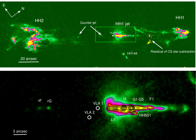
Figure 1: [Fe II] 1.64$\mu$m continuum subtracted image of the HH 1/2 region. The bottom panel is an enlarged view of the inner HH 1 jet region, marked by a green box in the top panel. Contour levels are at 1, 2, 3, 4, 6, 8, 10, 15 and 20$\times$10^-19 erg s^-1 cm^-2 Å^-1 pixel^-1.

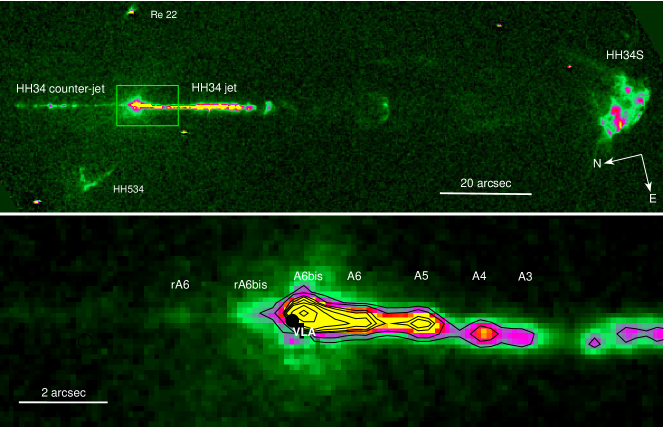
Figure 2: The same as Fig. 1 for the HH 34 region. Contour levels are at 1.2, 2, 4, 5, 7, 10, 20 and 40$\times$10^-19 erg s^-1 cm^-2 Å^-1 pixel^-1.

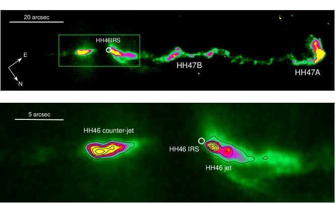
Figure 3: The same as Fig. 1 for the HH 46/47 region. Contour levels are at 1.3, 2.6, 4.9, 7.0, 10, and 15$\times$10^-19 erg s^-1 cm^-2 Å^-1 pixel^-1.

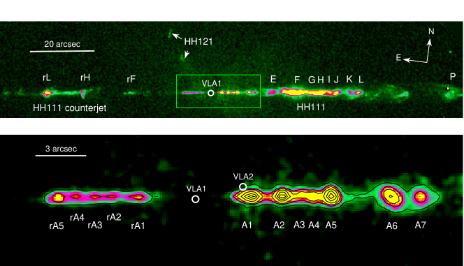
Figure 4: The same as Fig. 1 for the HH 111 region. Contour levels are at 0.2, 0.5, 0.8, 1.5, 2.5, 3.5 and 4.5$\times$10^-19 erg s^-1 cm^-2 Å^-1 pixel^-1.

Figure 1 shows the image of the HH 1 and HH 2 region, that includes the HH 1 (blue-shifted) jet, driven by the radio source VLA1. The other radio source of the system, VLA2, driving the HH 144 outflow, is also indicated. Few weak knots of the counter-jet are also observed here. In the bottom panel, a region covering the HH 1 jet is enlarged. Here we see that the jet is detected as close as 2$\farcs$5 from the driving source while the innermost region is obscured due to high extinction, consistent with previous reports by Reipurth et al. (2000a); Davis et al. (2000); Nisini et al. (2005). Various jet knots are labelled from L to F following the nomenclature of Reipurth et al. (2000a). The HH 501 knots, which differ in orientation with respect to the main HH 1 jet knots, are also labelled. The two knots in the red-shifted HH 1 counter-jet, correspond to similar distances from the source as knots G and F, and so are here labelled as rG and rF.

Figure 2 shows the HH 34 jet and associated HH34S bow shock to the south. The red-shifted counter-jet is clearly detected, at variance with optical and even [Fe II] 1.25$\mu$m images. Stapelfeldt et al. (1991) first imaged the HH 34 jet in the NIR [Fe II] 1.64$\mu$m line, and also faintly detected the counterjet (see Figure 7f in their paper). The counterjet was detected in further IR spectroscopic and imaging observations (Garcia Lopez et al., 2010; Antoniucci, S. et al., 2014) and Spitzer images (Raga et al., 2011), but never with the level of details shown here. The bottom panel shows the various observed jet knots, which are labelled following the nomenclature of Reipurth et al. (2002). The jet driving source, VLA, is also marked.

Figure 3 shows the complex structure of the HH 46/47 target, which was first observed in the NIR by Eislöffel et al. (1994). Our image covers most of the blue-shifted outflow, that includes the HH 46 jet and its red-shifted counter-jet, the HH 47B knots chain, and the bright bow shock towards the North-East, HH 47A. The position of the jet driving source, HH 46 IRS, is also marked. The enlarged figure of the continuum subtracted central region shows the detailed structure of the inner jet better than previous optical and IR HST images as these were dominated by the strong reflection nebula in which the jet is embedded (Reipurth et al., 2000a; Hartigan et al., 2005). In fact, significant residual scattered line emission is still visible in the image on the northern side of the jet. Bright jet knots are seen that follow the arc-shaped structure of the jet. The red-shifted jet does not emerge until about 5 arcsec from the central source and it is not symmetrically displaced with respect to the blue-shifted jet.

Figure 4 shows the HH 111 bipolar jet, driven by the radio source VLA1 with the bright blue-shifted lobe and its dimmer red-shifted counterpart. Many individual knots are revealed in the enlarged view of the inner jet region. Near the HH 111 jet we observe also knots from the HH 121 jet, driven by the VLA2 radio source. The [Fe II] 1.64$\mu$m image reveals many details of the jet structure within $\sim$ 20 arcsec from the driving source (VLA1) that remained hidden in optical images, where the jet is seen only at larger distances (knots from E to L, Reipurth et al., 1997; Hartigan et al., 2001), when it emerges from a cone-shaped cavity. This is shown in Fig. 5, where the image taken in the F167 continuum filter is presented, with superimposed contours of the [O I] emission.

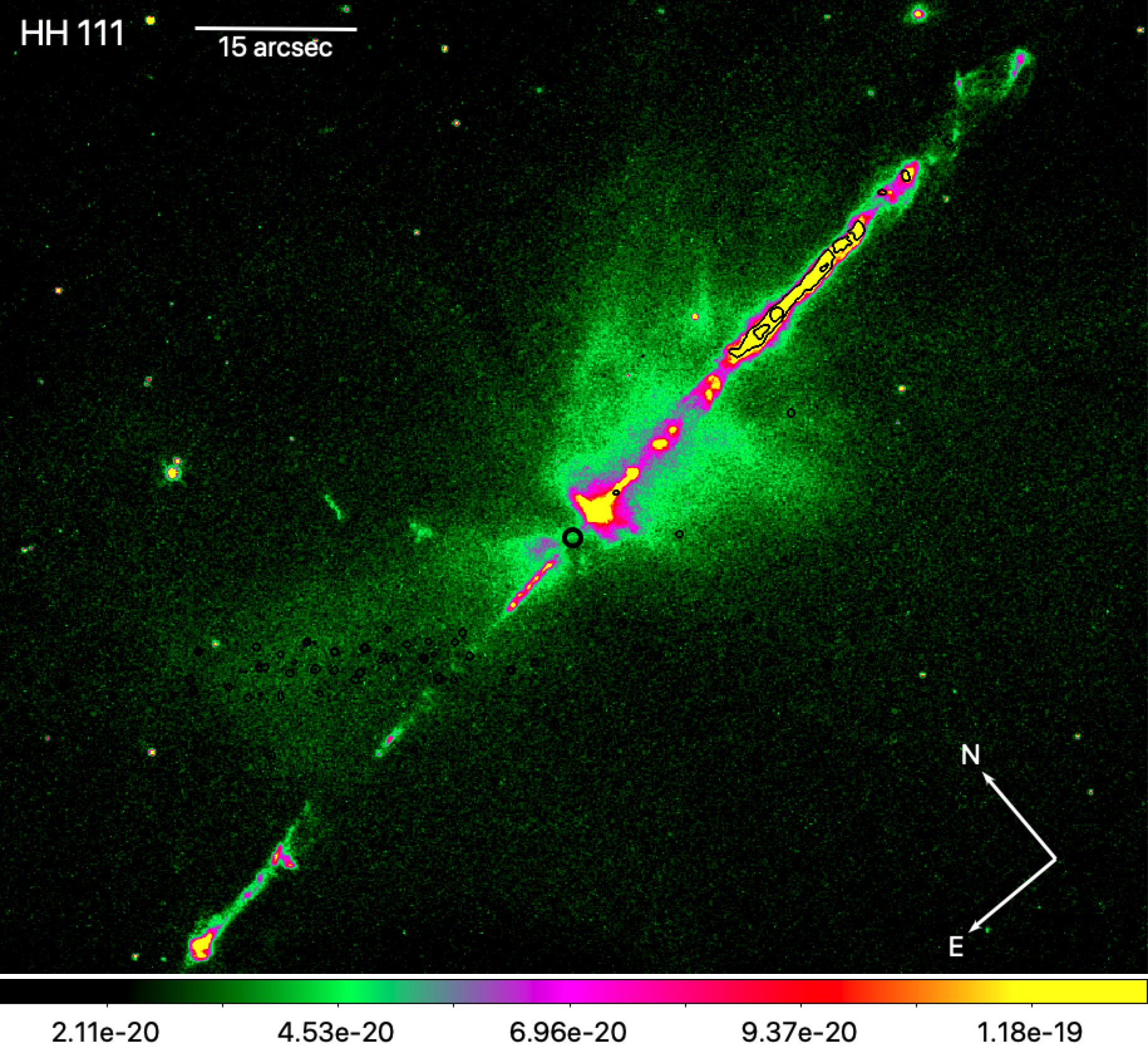
Figure 5: [Fe II] 1.64$\mu$m line+continuum image of the HH 111 jet and cavity. [O I] contours are overplotted in black (levels are 0.2 and 1 $\times$10^-19 erg s^-1 cm^-2 Å^-1 pixel^-1), showing that at optical wavelengths the jet is observed only at large distances from the source (marked by the black circle). The red-shifted jet is not detected in the optical.

Some of the red-shifted knots observed here were already discovered in previous HST/NICMOS and Spitzer images of the jet (Reipurth et al., 2000a; Noriega-Crespo et al., 2011a) as well as in ground-based 2.12$\mu$m observations (Coppin et al., 1998). However, our continuum subtracted image, where the large nebulosity around the central source is removed, reveals the sequence of symmetric blue- and red-shifted knots with an unprecedented level of detail. We name the inner knots, observed only in the IR in the blue-shifted jet, A1 - A7. We name corresponding counter-jet knots rA1 - rA5.

3.1.2 Proper Motions

We compare the [Fe II] images of our targets with archival images taken in previous epochs with HST in the [S II] filter (top two panels of Figures 6-8). The [S II] images of the HH 34 and HH 46 jets used here were first published in Hartigan et al. (2011); and for HH 111 we use the [S II] image from Hartigan et al. (2001).

The jet morphology, when both lines are detected, is very similar with only minor changes in individual knots. The major difference between the two tracers is that [Fe II] emission is observed close to the source, unlike [S II]. This is particularly evident for HH 111 (see Figure 8), where [S II] is observed only where the jet emerges from the cone-like cavity.

As the [S II] images were taken typically 10-20 years before the [Fe II] images, combining the two datasets allows us to measure the secular proper motions of the jets with great accuracy, as although the tracers are different, the [S II] and [Fe II] emission is expected to peak in the same post-shock region for a given epoch (Nisini et al., 2005).

Firstly, the [Fe II] and [S II] images were registered to each other using field stars detected in both filters. For HH 1 however, only one star in common was found in the two fields, therefore it was not possible to align the images. We therefore report on the proper motion for the HH 34, HH 46/47 and HH 111 jets only. The images were also rotated such that the direction of the flow was aligned to the horizontal according to the jet PAs listed in Table LABEL:table:targets, and defined on the inner jet/counter-jet knots. The proper motions were derived by measuring the shifts between the individual knots in the [Fe II] and [S II] images. These shifts are clearly observed in the [Fe II] - [S II] difference images for each target as presented in the bottom panels of Figures 6-8. We identified knots that do not present major structural changes between one epoch and the next, and we measure the difference in position between the photo-centres of the knots in the two epochs. Proper motions converted to tangential velocities using the adopted distance, together with values reported in recent literature based on a smaller time interval corrected for our adopted distance, are presented in Figure 10 and listed in the tables of Appendix C

For the HH 34 jet, the measured tangential velocities (top panel of Figure 10) tend to decrease with distance from the source, as already reported by Raga et al. (2012), with differences of within 20-30 km s^-1 in most of the knots. Ground based images of the HH 34 jet (Eislöffel & Mundt, 1992) report a similar trend for the inner part of the jet, however a large increase in tangential velocity was measured further from the source which is not seen in our results. At the position of about 5$\arcsec$, we see an abrupt decrease of tangential velocity which is not recorded by Raga et al. However, the same rapid decrease at similar distances is measured in previous proper motion studies by Eislöffel & Mundt (1992) and Reipurth et al. (2002).

For the HH 111 jet, the tangential velocities decrease with distance in the first 40$\arcsec$ from the star, with small fluctuations of about 15-20 km s^-1. This trend was also found by Hartigan et al. (2001), with higher absolute values by approximately 20-30 km s^-1. The velocity seems then to increase again at further distance from the star.

The deceleration of jets with distance is a known phenomenon observed in several extended outflows. It has been interpreted as either due to an intrinsic variability of the ejection velocity or to a braking in the interaction of the jet with the surrounding medium. Jet precession was also suggested as a possible cause for the jet slow down (e.g. Masciadri et al., 2002).

At variance with the other two outflows, the HH 46/47 jet appears to be accelerating with distance from the star. If we exclude the knots at 40$\arcsec$ and 70$\arcsec$, the derived tangential velocities correspond to those found by Hartigan et al. (2005) within 20 km s^-1. Ground based images (Eislöffel & Mundt, 1994) measure similar tangential velocities which generally remain more constant along the jet length.

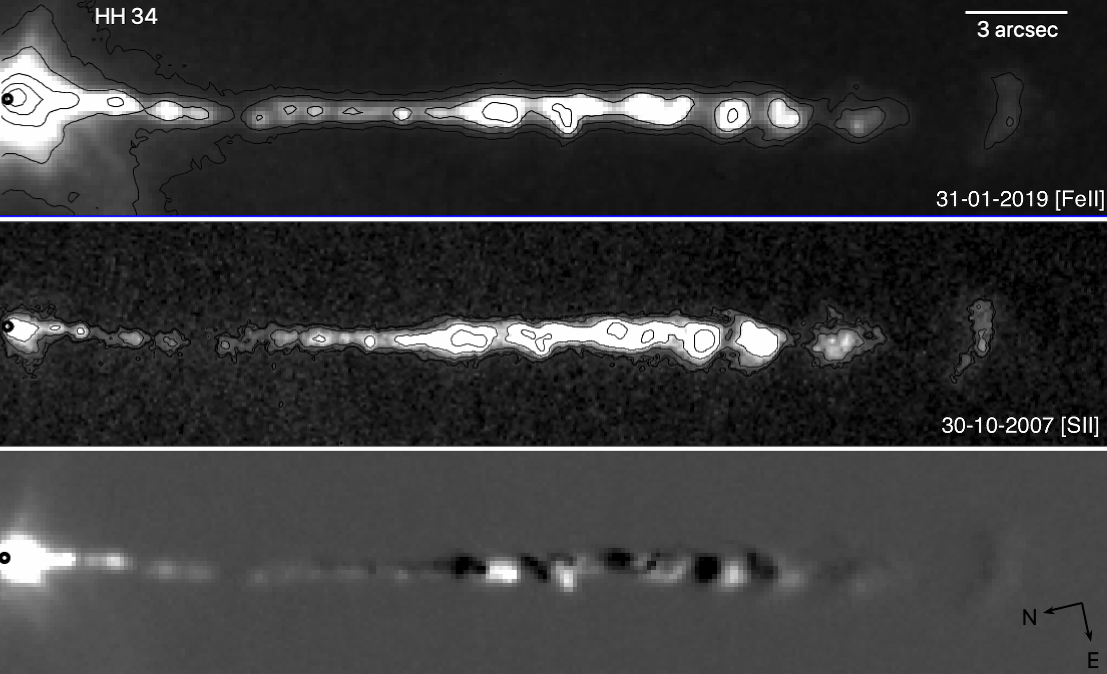
Figure 6: Comparison of the HH 34 knot positions in [Fe II] with contour levels at 0.05, 0.08, 0.19, 0.67, 2.5 and 9.9 $\times$10^-18 erg s^-1 cm^-2 Å^-1 pixel^-1. (top) and [S II] with contour levels at 0.6, 0.63, 0.74, 1.2, 2.9 and 9.9 $\times$10^-16 erg s^-1 cm^-2 Å^-1 pixel^-1. (middle) images with an eleven year baseline. The circle marks the driving source position. The bottom panel shows the subtraction image for [Fe II]-[S II]

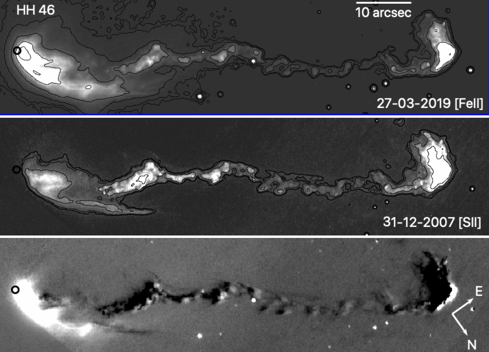
Figure 7: Same as Fig. 6 for the HH 46 outflow. [Fe II] contour levels are 0.2, 0.23, 0.35, 0.8, 2.6 and 9.9 $\times$10^-19 erg s^-1 cm^-2 Å^-1 pixel^-1. [S II] contour levels are 0.9, 0.94, 1.1, 2.5 and 9.9 $\times$10^-16 erg s^-1 cm^-2 Å^-1 pixel^-1.

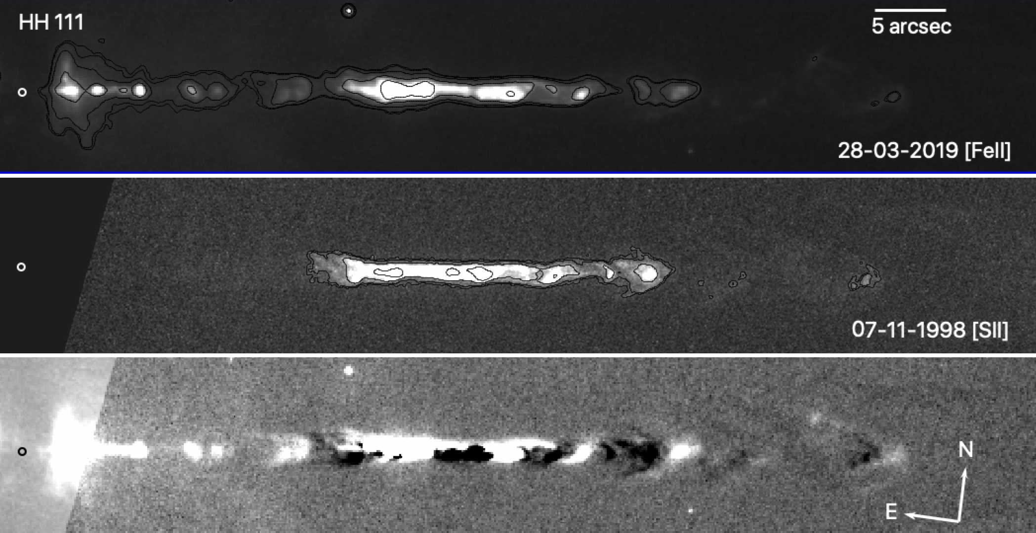
Figure 8: Same as Fig. 6 for the HH 111 outflow. [Fe II] contour levels are 0.55, 0.58, 0.75, 1.7 and 7 $\times$10^-19 erg s^-1 cm^-2 Å^-1 pixel^-1. [S II] contour levels are 0.1, 0.12, 0.25, 0.9 and 5 $\times$10^-15 erg s^-1 cm^-2 Å^-1 pixel^-1.

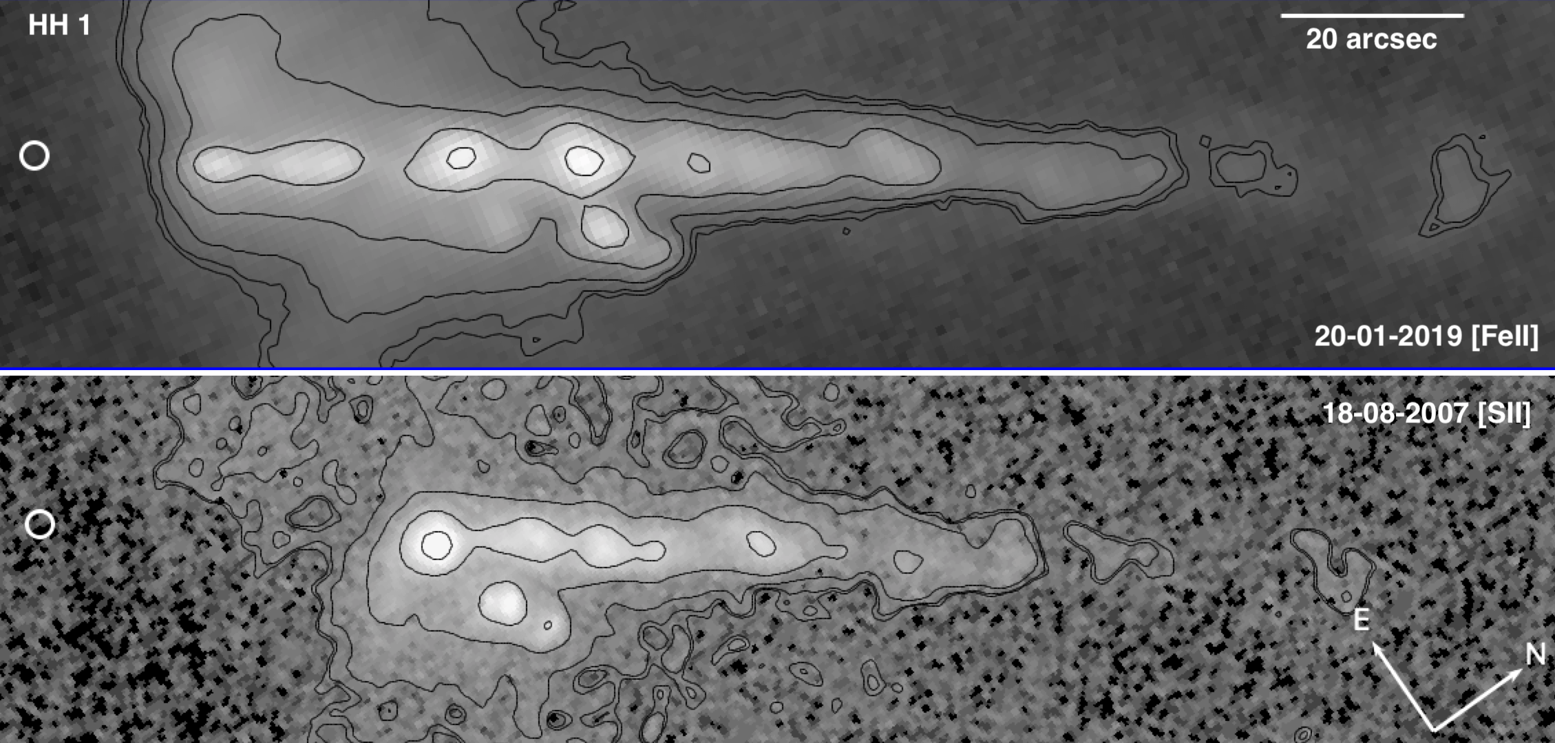
Figure 9: Comparison of HH 1 [Fe II] (top) and [S II] (bottom) images with an eleven year baseline. Only one star is present in both images so it was not possible to accurately align the images to create the subtraction image. However, we still see the jet in the [Fe II] image is detected much closer to the star than in [S II]. [Fe II] contour levels are 0.07, 0.08, 0.1, 0.25, 0.8 and 3 $\times$10^-18 erg s^-1 cm^-2 Å^-1 pixel^-1. [S II] contour levels are 0.4, 0.42, 0.5, 0.8, 2 and 7 $\times$10^-15 erg s^-1 cm^-2 Å^-1 pixel^-1.

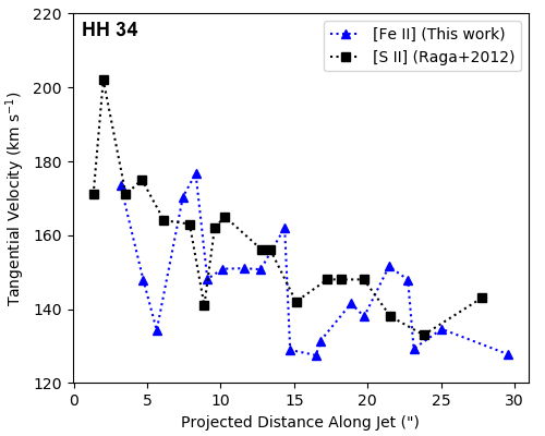
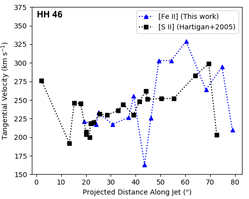
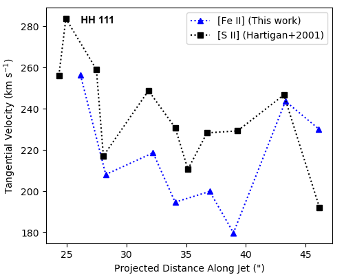
Figure 10: Tangential velocities for HH 34 (top), HH 46 (middle) and HH 111 (bottom). The black markers show literature values, while the blue markers are the values found from the [Fe II] knot positions in this work.

3.2 Inner Jet Region

HST infrared images allow us to trace the jet targets closer to the central source than was previously possible with optical images, and to detect the fainter counter-jet in all cases. These images can therefore provide insights into some properties of the inner jet region which have so far remained unexplored. In this section we analyse the width of the jets and its variation with distance from the central source, the symmetry between the jet and the counter-jet, and the extinction in the inner jet region.

3.2.1 Jet Collimation

The degree of collimation of the jets can be estimated by measuring how the jet width varies with distance from the driving source. In order to measure the jet width, the continuum-subtracted [Fe II] 1.64 $\mu$m images were first rotated to align the jet PA with the x-axis (see Section 3.1.2). Two approaches were then considered. In the first, we measured the jet width as the FWHM of the transverse intensity profile with a single or double Gaussian, depending on the presence of low-intensity wings. The second approach, was to directly measure the width of the transverse intensity profile at half the height of the peak, without Gaussian fitting. The two methods give similar results within the errors. In some cases, as in HH 1 at the position where the HH 501 knots intersect the main jet, a triple-Gaussian fit was required. Lastly, the jet widths were deconvolved by subtracting in quadrature the instrumental FWHM of 0$\farcs$153.

Figure 11 shows the measurements of jet widths for each of the targets as a function of distance from the central source. For comparison, the binned flux along the jet is plotted in the top panels. In all cases, a gradual increase in jet width with distance is found, with an undulation in the jet width for the HH 1 and HH 111 jets, anticorrelated with the intensity. This effect is due to the fact that in the dimmer points the residual nebulosity dominates the emission and consequently the jet FWHM is overestimated. This undulation is not observed at HH 34 or HH 46. In all cases, the jet width could not be measured closer than $\sim$100 au to the star either because of a lack of jet emission, or residual continuum emission close to the star.

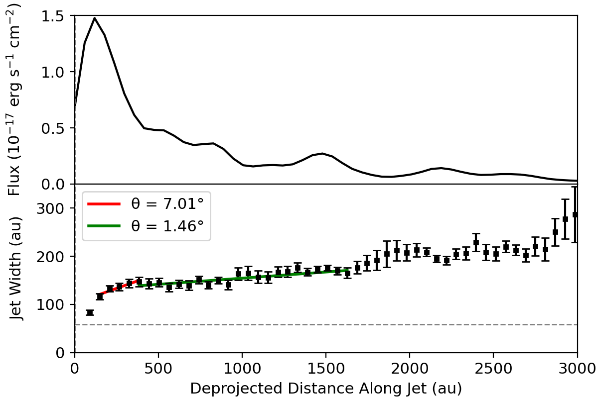
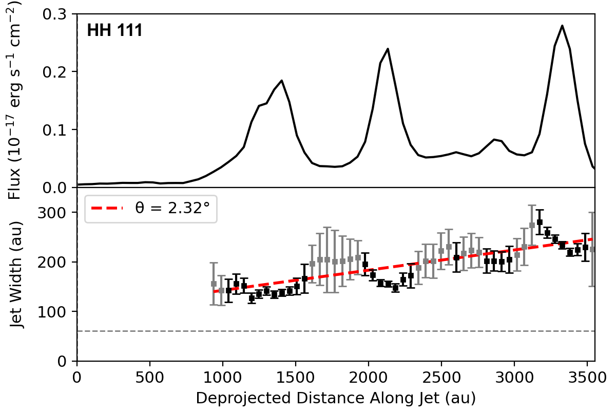
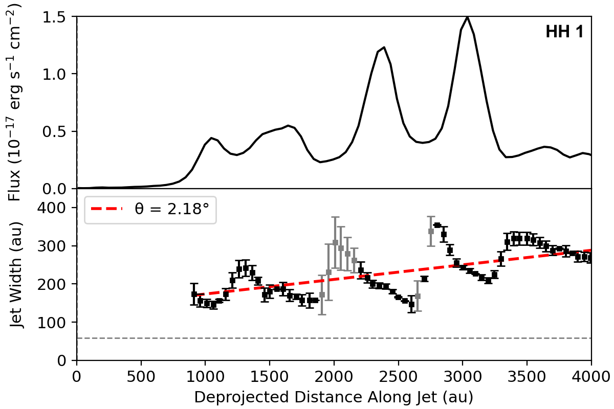
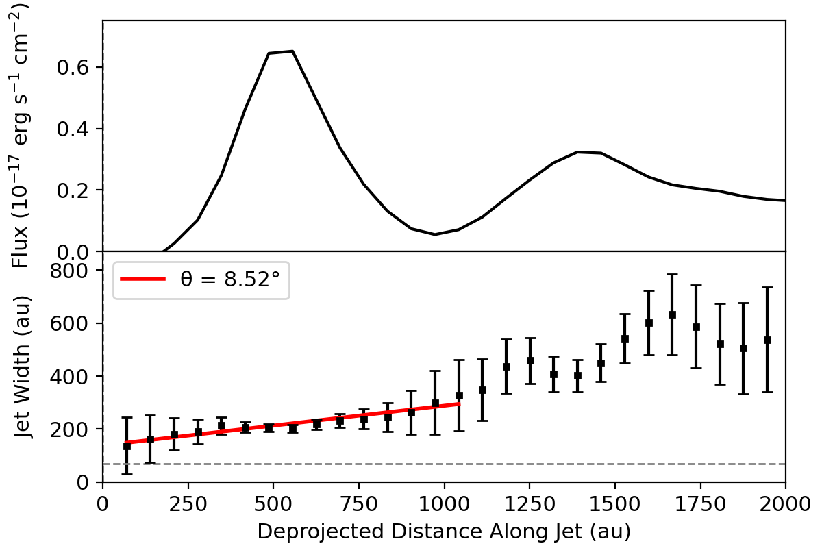
Figure 11: Top: Binned flux along the jet. Bottom: Jet FWHM from 1D Gaussian fits at each pixel. Errors are 3$\sigma$. In HH 34, we measure the opening angle with a linear fit over the regions in the jet marked by red and green solid lines. In HH 46, the opening angle is measured at every point along the jet up to approx 1000 au, marked by the solid red line. For HH 1 and HH 111, the opening angle is measured by fitting all points with a 3$\sigma$ smaller than 30 au (dashed red lines). The grey points in for HH 1 and HH 111 are those with 3$\sigma$ larger than 30 au, which are not fitted when measuring the opening angle. The dashed grey line is the instrumental FWHM of 0$\farcs$153.

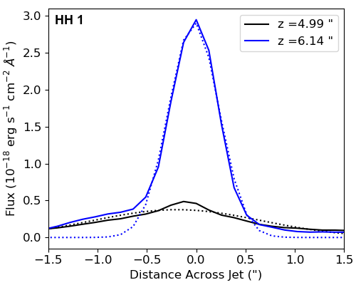
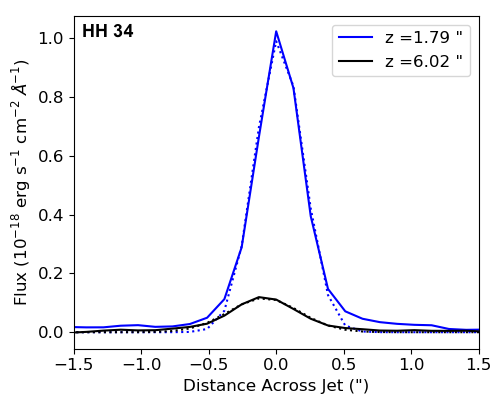
Figure 12: Top: Comparison of the brightness profile and 1D Gaussian fits for two sample positions along the HH 1 jet. The dim profile (black) shows how the jet width may be overestimated by the presence of low intensity emission, leading to the undulating pattern of the jet width seen in Figure 11. Bottom: Comparison of the brightness profile and 1D Gaussian fits for two sample positions along the HH 34 jet which does not appear to be affected by residual low intensity emission.

The observed expansion of the de-projected jet width with distance gives a measure of the opening angle of the jet. As shown in Figure 11, opening angles of $\approx$ 2^∘ are found for the outer regions of the jets (i.e. at deprojected distances larger than a few hundred au from the source). However, for HH 46, we observe a wider opening angle of $\approx$ 8.5^∘. Furthermore, for HH 34 we observe a change in opening angle, where in the innermost part of the jet we measure an opening angle of 7^∘, decreasing to 1.5^∘ measured between $\approx$ 400 - 1500 au from the star. Table 3 provides the values measured for each target.

Estimates of the widths for individual knots of the HH 1, HH 34 and HH 111 jets were given from previous HST images in Reipurth et al. (2000a), Reipurth et al. (2002), Reipurth et al. (2000b), respectively. However these works, which are based on images without continuum subtraction of the source nebulosity, mainly addressed jet collimation at larger distances from the source. In Reipurth et al. (2000a, b) the jet widths and opening angles of HH 111 and HH 1 were measured for images in both [S II] and [Fe II] emission, the latter being acquired with HST/NICMOS observations. In HH 111, these previous measurements give a width of about 150 au at a distance of $\sim$ 1200 au, i.e. compatible with our estimates. For HH 1, Reipurth et al. (2000b) derive a width of about 80 au at a distance of 1000 au, but we measure about 150 au. Meanwhile, at larger distances (e.g. knot H and G) there is better agreement. For the HH 34 jet, Reipurth et al. (2002) report a variation of the [S II] width with distance. Their measured widths are smaller than ours for the inner knots (at $<$ 2 arcsec from the source), while at larger distances the two become comparable. We think that these differences are caused by the increased difficulty in separating the jet from the source nebulosity in images where the continuum is not subtracted.

Table 3: Opening angles for each target measured over various distances along the jet

Target	z	Opening angle
	(au)	(∘)
HH 1	>1000	2.2
HH 34	<400	7.0
	400 - 1500	1.5
HH 46	<1000	8.5
HH 111	>1000	2.3

3.2.2 Jet/counter-jet asymmetries

Since we observe both jet and counter-jet in all sources, we can investigate asymmetries between them. To this aim, we have mapped the jet and counter-jet trajectory, identifying the position of each jet knot photocentre by using a 2D Gaussian fit. The errors on the knot centroids were found using 1D Gaussian fits across the jet. We considered only the knots in the main body of the collimated jets, as they are more compact and thus their centroids are less prone to uncertainty caused by the presence of diffuse emission, unlike in extended bow shocks at the jet apex. The knot positions with respect to the jet axis (defined according to the PA given in Table 1) are plotted in Figure 13. The driving source position has been taken as the origin of the jets. All jets show a systematic displacement with respect to their axis. For HH 34 and HH 111, the driving source position, taken as coincident with the VLA sources, appears shifted by about 0$\farcs$1 with respect to the jet axis. It is unlikely that this is an effect due to extinction, since we use the radio source coordinates which should not be affected by diffuse emission, therefore this apparent shift indicates a possible misplacement of the source coordinates with respect to the HST images.

In HH 111, HH 34 and HH 46, we observe symmetry between the corresponding blue- and red-shifted knots with respect to the plane perpendicular to the jet passing through the source. In particular, the HH 111 jet is very well traced at distances up to $\pm$ 60$\arcsec$ from the central source and both the jet and counter-jet show mirror symmetry in their trajectories. This configuration can be caused by the orbital motion of the jet source around a companion, as we will discuss in Section 4.2. In HH 34 and HH 46, while the blue- and red-shifted knots also appear to show mirror symmetry, we cannot identify a clear undulation with a jet/counter-jet symmetry. Therefore, we cannot exclude other possible causes of the observed pattern given the large error bars in the red-shifted knots (for HH 34) and the low number of knots (for HH 46). For HH 1, an insufficient number of red-shifted knots are observed to allow differentiation between mirror symmetry and point symmetry patterns in the trajectory. Note, however, that identifying the exact jet PA using the inner knots is tricky, and can significantly influence the interpretation of the asymmetry. We will discuss the observed asymmetries in more detail in Section 4.2.1.

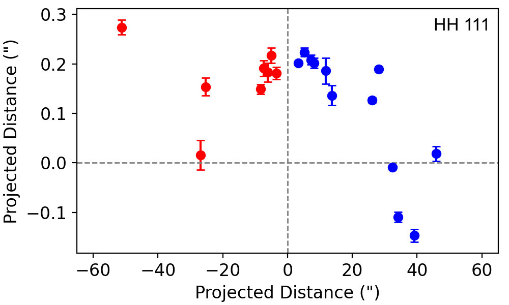
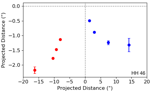
Figure 13: Position of the 2D photocentres of knots along the jets with respect to the jet axis and the plane perpendicular to it passing through the source (horizontal and vertical grey dashed lines, respectively). Error bars are 1$\sigma$.

3.3 Extinction along the jets

The [Fe II]1.25 $\mu$m/1.64 $\mu$m line ratio is independent on the gas physical conditions (temperature and density), since the two lines originate from the same upper level. Consequently, this ratio depends only on the atomic physics and on the reddening along the line of sight. We can therefore use our maps obtained in the two narrow band filters to estimate the extinction along the jet. This method assumes that the emission entering our narrow band filters is only due to the reddened lines. However, as already noted, close to the source there is a significant contribution from nebulosity due to continuum scattered light. Therefore, we measured the line ratio using images which were first continuum-subtracted. The presence of fainter [Fe II] lines falling within the bandwidth of the continuum filter can also contaminate the continuum-subtracted flux measurements. We evaluate this contamination in the Appendix D and estimate it to be 5% at most in the dense jet sections close to the source.

To measure the line ratio along the length of each jet, the jet images were binned across the width of the jet, producing the 1D line flux curves in Figure 14. The extinction values were calculated by averaging the flux in each knot along the jet and assuming the empirically determined intrinsic value for the [Fe II]1.25/1.64 $\mu$m ratio of 1.1 (Giannini et al., 2015). The Cardelli et al. (1989) extinction law has been used to estimate $A_{V}$. The errors in the extinction calculation were taken to be 14% based on the HST/WFC3 PHOTFLAM calibration errors of 10%.

Figure 14 and Table 4 show high visual extinction values close to the source, typically 10-15 mag, that gradually decrease towards negligible values at further distances. In the inner regions, residuals of continuum emission and noise introduced by continuum subtraction may influence the results. Red-shifted counter-jets have consistently larger values with respect to the corresponding blue-shifted jets. In HH 34 and HH 1, where the counter-jet has been detected only in the 1.64 $\mu$m line, lower limits on the A_V of about 10 mag have been estimated.

Figure 14: Extinction curves for all four sources. Extinction values calculated from averaged flux values of the [Fe II] 1.25 $\mu$m and 1.64 $\mu$m lines, assuming a theoretical ratio value of 1.1 (Giannini et al., 2015). Upper limits were calculated at points where the SNR of the 1.25 $\mu$m line was less than 3.

Table 4: Extinction (A_ν) values along each of the four jets. The error is 14%.

HH 1		HH 34		HH 46		HH 111
z ($"$)	Aν (mag)	z ($"$)	Aν (mag)	z ($"$)	Aν (mag)	z ($"$)	Aν (mag)
-13.5	7.7	-25.47	8.1	-10.05	6.5	-42.82	3.69
-11.3	12.1	-21.7	8.5	-7.17	14.5	-40.19	3.57
2.11	10.9	-19.71	14.0	-4.99	21.5	-27.07	10.05
3.97	9.4	-17.73	15.9	-0.70	14.9	-25.02	8.49
5.76	3.1	-15.42	11.5	0.32	13.5	-8.51	12.68
7.23	2.3	-12.99	5.9	1.66	8.2	-5.70	16.01
		-2.56	6.6			-3.01	15.99
		1.41	4.7			2.69	14.43
		3.33	4.6			5.82	7.48
						8.32	6.57
						9.47	3.86
						12.16	2.67
						13.36	3.36
						14.59	2.60

4 Discussion

4.1 Comparing Class 0/I to Class II jet widths and collimation

Figure 15 compares the widths of our four jets measured in [Fe II] with those of T Tauri jets in the literature which are based on high spatial resolution observations (i.e. using HST or using ground-based observations with adaptive optics). The HH 1 and HH 111 widths appear only in the right panel of Figure 15 because we do not observe these jets close to the source. Similarly, the HH 46 jet is not shown in the right panel because it becomes wider than the y-axis range of the plot.

Our results directly compare with those of the T Tauri jets, which are based on [Fe II] or [S II] lines tracing the same parts of the jet, as we discussed in previous section.

As seen in Section 3.2.1, HH 34 and HH 46 have opening angles of $\sim$ 1.5 and 8.5 ^∘ (respectively) and this collimation, similar also for the other jets, is preserved up to very large distances. In HH 34, however, the widths measured in the first points at z $<$ 400 au suggest an initial wider opening angle of $\sim$ 7^∘ that however would need confirmation with observations at higher spatial resolution.

The more striking difference emerging from Figure 15 is that the HH 34 and HH 46 jet widths are much wider than for the T Tauri sources when compared on the same spatial scale. T Tauri jets actually show a wide range of jet widths, which also depend on the velocity component that one is analysing. In DG Tau, for example, spectro-imaging observations show that the jet component at high velocity (the HVC in Figure 15) is narrower and more collimated than the component at medium velocity (the MVC Agra-Amboage et al., 2011; Maurri et al., 2014). In any case, the velocity integrated widths measured on HH 34 and HH 46 are a factor of 2-3 larger than those estimated for the wider DG Tau velocity component. From Figure 15, we also note that the widths measured on the Class 0 source HH 212 by means of SiO observations (Lee et al., 2017) is in line with the values measured on T Tauri stars, which suggests that jet collimation does not necessarily depend on evolution.

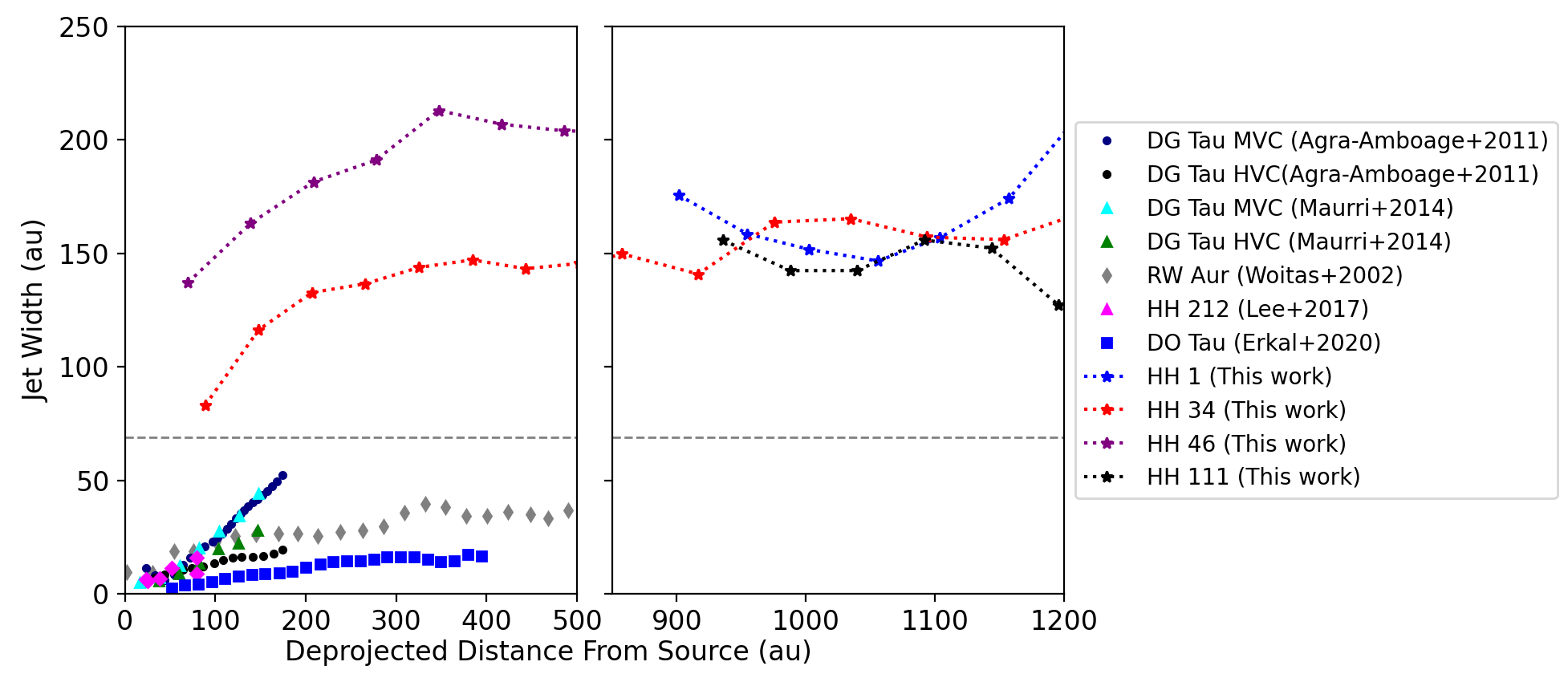
Figure 15: Comparison of Class 0/I jet widths derived in this paper with the widths measured for several T Tauri jets in the literature. The horizontal dashed line is the instrumental FWHM (0.153$\farcs$) in our measurements.

Given our measured widths at a distance of $\sim$ 100 au, a simple linear extrapolation of the observed jet opening angle back to the disk plane would project an initial diameter of about 70 au and 125 au for HH 34 and HH 46, respectively. These represent upper limits on the jet launching regions, if one considers magneto-centrifugal mechanisms where the jet initially expands and is then recollimated at few au above the disk (e.g. Pelletier & Pudritz, 1992). Estimates of jet launch radii performed through observed jet rotation give values between 0.1-4 au for the high velocity atomic component of T Tauri jets (Bacciotti et al., 2002, Coffey et al., 2004, 2007), while for the Class I sources HH 26 and HH 72 Chrysostomou et al. (2008) measured slighting larger launch radii of 2-4 au through H₂ observations. Also, HST observations of the HN Tau and UZ Tau E jets indicate an original width at the jet source $<$ 5 au (Hartigan et al., 2004). If we assume that the HH34 and HH46 jets originate from similar launching radii at $<5$ au, then the widths measured at 100 au distance imply that the jets should initially undergo a fast expansion with an opening angle of $>$ 40 degrees.

An additional possibility is that at large distance we are not measuring the intrinsic jet diameter but rather the width of internal, unresolved, bow shocks or that the width appears larger because of the additional contribution from envelope material entrained in a turbulent mixing layer (e.g. Binette et al., 1999). Observations at higher spatial resolution would be needed to explore the various possibilities.

4.2 Asymmetric lobes

There are several studies in the literature which together show that protostellar jets are rarely well-centred on their propagation axis. In many cases, jet knots exhibit a regular wiggling pattern that cannot be explained by a change in the trajectory of the jet due to obstacles along the path. Alternatively, observed wiggling may be due to variations in the direction of the ejection at the jet origin. Such direction changes can have various causes. The possibility that the observed undulations are due to a misalignment of the jet axis with the source rotational axis is generally ruled out, because it would produce precession on timescales which are too short. It is more likely that the wiggling originates from the presence of one or more companions, in which case the wiggling pattern may be due either to the orbital motion of the driving source around the companion, or to precession of the disk plane due to tidal interactions in non co-planar binary systems (e.g. Masciadri & Raga, 2002; Terquem et al., 1999). These two scenarios can be disentangled through examination of the symmetry pattern of the trajectory presented by the jet and counter-jet with respect to the central source: a mirror-symmetry in the case of orbital motion, and a point-symmetry in the case of precession.

The jet/counter-jet symmetry has been studied in many sources, both Class II (T Tauri) and Class 0/I. Mirror-symmetric jets seem more common than point-symmetric jets (e.g. Noriega-Crespo et al., 2020; Estalella et al., 2012) although well-known examples of precessing jets have been observed, e.g. the Class 0 outflows L1157 (Gueth et al., 1996; Takami et al., 2011) and Cep E (Eislöffel et al., 1996). In our study, we find that three out of four targets (i.e. HH 34, HH 111 and HH 46) show mirror-symmetry in the red- and blue-shifted knot positions. However, as noted in Section 3.2.2, we find some evidence of a mirror-symmetry pattern caused by orbital motion of the jet source only for HH 111, due to the difficulty in identifying a clear wiggling pattern in HH 34 and HH 46. In the HH 1 jet (see Figure 13), the detected red-shifted knots are too few and faint to ascertain the type of symmetry.

The HH 46 blue-shifted outflow has a very pronounced large scale helicoidal pattern. Masciadri & Raga (2002) interpreted this pattern as due to the orbital motion of the jet source around the companion found by Reipurth et al. (2000b) at $\lambda\sim 2\mu$m with a separation of approximately 120 au. Both Masciadri & Raga (2002) and Reipurth et al. (2000b) however conclude that the complex morphology of the outflow cannot be reproduced by this simple interpretation and could require the presence of a triple system.

For HH 34, the symmetry between the jet and counter-jet was discussed in Raga et al. (2011), where the counter-jet at distances $>$ 5$\arcsec$ was for the first time revealed by means of Spitzer observations. They observed an offset in the positions of corresponding jet/counter-jet knots, and interpreted it as due to a velocity difference and a time delay in ejection between the corresponding knot pairs.

We now observe the HH 34 counter-jet at a higher spatial resolution and closer to the source than was previously possible. In order to better compare the knot displacement in the two lobes, we show in figure 16 the offsets as a function of distance, where the positions of the red-shifted knots have been folded over so as to be plotted on the same x-scale as the blue-shifted knots. Note that, for both the blue and red data-points, there is a sharp increase of the offsets with respect to the jet axis for distances $<\sim$ 10$\arcsec$. However, this increase in offsets occurs much more rapidly in the blue-shifted jet, followed by an abrupt change in direction at about 7$\arcsec$ after which the jet and counter-jet axes seem to align. It is not clear whether such a sharp kink of the jet axis exists in the counter-jet, because the corresponding region is extincted by the large nebulosity and so the jet trajectory cannot be well traced in this region. Although the knots do not follow a straight trajectory, it is difficult to identify any clear undulation with a jet/counter-jet symmetry. Jet/counter-jet knot positions are also slightly shifted with respect to each other, but we cannot find evidence of any regular pattern in these shifts.

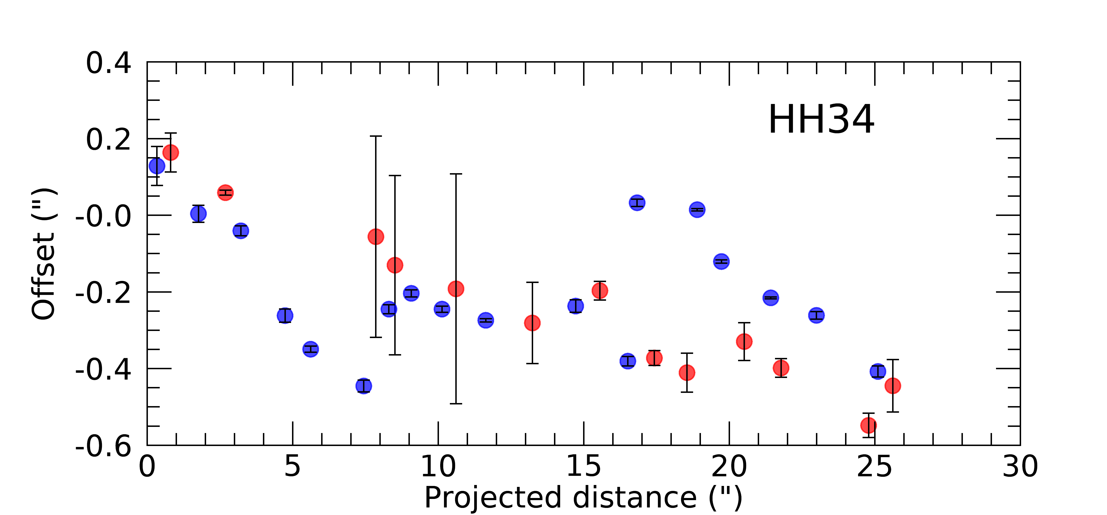
Figure 16: Offsets of the knots in the HH 34 jet (blue) and counter-jet (red) with respect to the jet axis originating from the VLA driving source. The counter-jet knot positions have been folded to be superimposed on the jet distance scale.

4.2.1 Modelling the orbital motion of HH 111

The HH 111 jet shows a clearer symmetry between jet and counter-jet, with a defined mirror-symmetric pattern. Such a symmetric pattern was noticed by Noriega-Crespo et al. (2011b), who studied the positional distribution of the jet knots in both lobes observed by Spitzer. Thanks to our higher spatial resolution, we can interpret the observed pattern as orbital motion of a binary system.

We model the spiral pattern seen in HH 111, adopting the formulation given in Anglada et al. (2007) and Masciadri & Raga (2002) for a ballistic jet of a star in circular orbit, assuming a constant jet velocity. The parameters that enter into the model are directly linked to observable quantities. In particular, the orbital radius of the jet source around the binary centre of mass, $r_{o}$, is given by:

$$r_{o}=\frac{\lambda\,\rm{tan}\,\alpha}{2\pi}\,D$$ (1)

where $\lambda$ is the angular distance in the plane of the sky between the positions of two maximum elongations, $\alpha$ is the half opening angle of the jet and $D$ is the distance. In addition, if $v_{j}$ and $v_{o}$ are the velocities perpendicular and parallel to the orbital plane, their ratio is given as:

$$k=v_{j}/v_{o}={\rm tan}\,\alpha\,{\rm cos}\,\phi=v_{t}/v_{o}$$ (2)

where $\phi$ is the inclination angle of the jet with respect to the plane of the sky, and $v_{t}$ is the jet tangential velocity.

Once $r_{o}$ and $v_{o}$ are measured, the orbital period $\tau_{o}$ can be also given by:

$$\tau_{o}=2\pi\,r_{o}/v_{o}$$ (3)

In addition, if $m_{1}$ is the mass of the jet source and $m_{2}$ the mass of the companion, we have :

$$m=m_{1}+m_{2}=\mu^{-3}\,{r_{o}}^{3}\,{\tau_{o}}^{-2}$$ (4)

where $\mu$ is $m_{2}/m$. Finally, the binary separation $a$ is given by $r_{o}/\mu$.

For our model of the the HH 111 jet, we assume a distance of 400 pc and $v_{t}$ = 320 km s^-1, i.e. the jet velocity at origin, estimated by extrapolating the tangential velocities measured along the jet in Section 3.1.2. An opening angle and $\lambda$ value of 2^∘ and 20$"$, respectively, are given as initial guesses for the model. Finally, we allow a slight change in the position of the driving source and the jet inclination in order to adjust the alignment with the jet axis.

We first tried to fit the observed offsets measured along the $\pm$ 60$\arcsec$ length of the jet with the binary orbital model described above. However, we could not find a good solution that reproduced the observed wiggling for all the knots. We then fitted only the internal knots ($\pm$ 20$\arcsec$), and the result is shown in Figure 17 where the best fit is superimposed on the observed offsets. We note that the more external knots show the same amplitude and period predicted by the fitted curve, but they are out of phase with respect to expectations. This behaviour is consistent with the decrease in velocity seen in Figure 10.

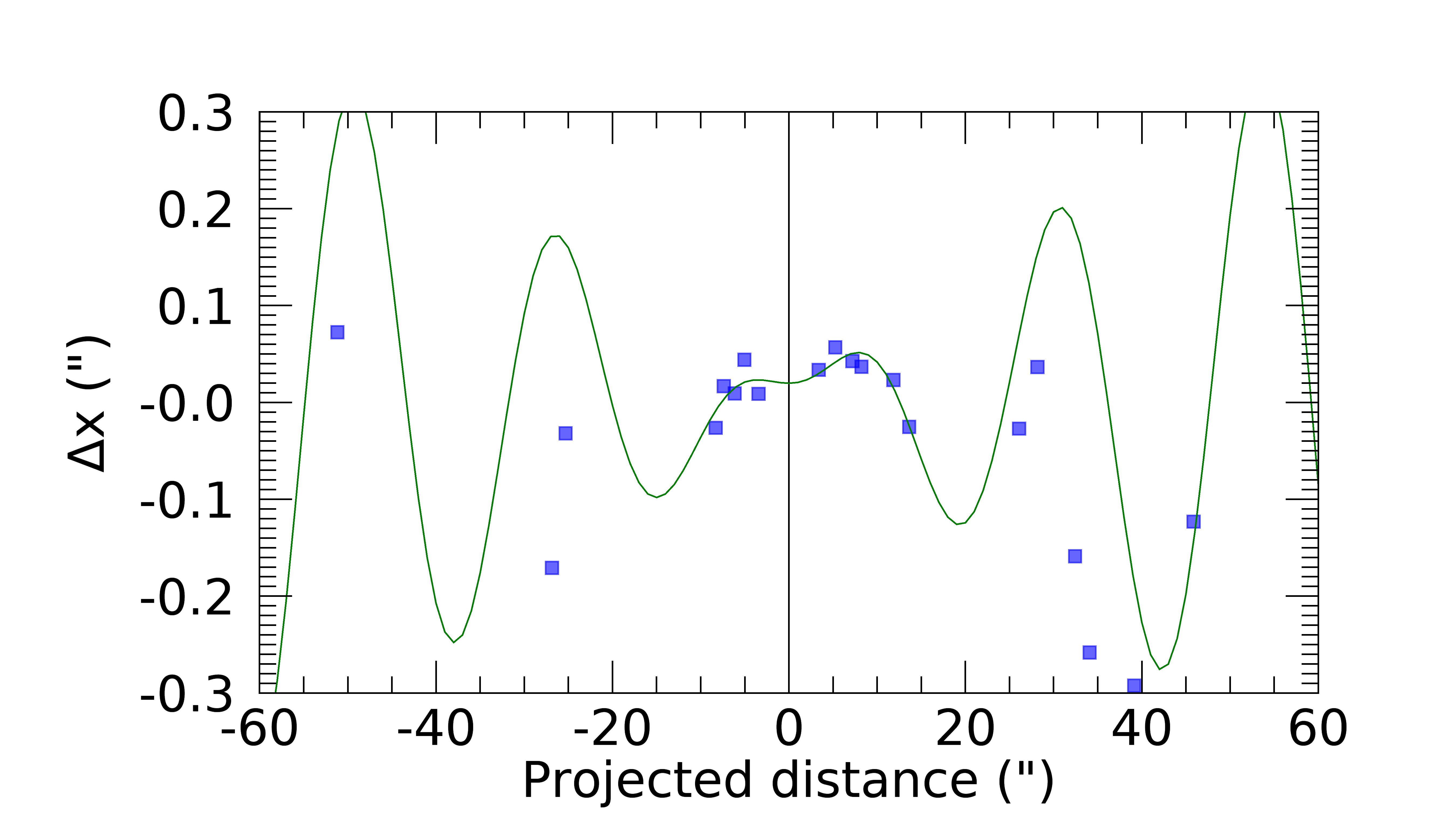
Figure 17: A model fit to the observed photocentre offset positions of the HH 111 inner knots as a function of distance from the exciting source. Blue boxes indicate the measured offsets. The solid green line is the best fit of the internal knots wiggle produced by an orbital motion of the jet source around a companion.

Table 5: Parameters of the orbital motion model for the inner knots.

Assumed parameters
$v_{t}$	320 km s-1
Mtot	1.0-2.0 M⊙	Lee et al. (2020)
$D$	400 pc	Lee et al. 2016
Derived parameters
$m_{1}$	0.8-1.4 M⊙
$m_{2}$	0.4-0.6 M⊙
Separation $a$	28-33 au
Period $\tau_{o}$	140 yr
Orbital velocity $v_{o}$	2.0 km s-1

The model fit gives as output $v_{o}$, $r_{o}$ and $\tau_{o}$. ALMA observations give an estimate for the mass of the VLA 1 source of 1.5$\pm$0.5 M_⊙. Assuming this value as the total mass of the binary, we derive, from equation (4) the masses of the individual sources and their separation (a=$r_{o}$/$\mu$).

Table 5 summarises all the assumed and derived parameters that we find by fitting the binary orbital model to the offsets of the inner knots for HH 111. Allowing for the total mass to lie in the range 1 - 2 M_⊙, the mass of the primary is in the range 0.8 - 1.4 M_⊙ and the mass of the secondary is in the range 0.4 - 0.6 M_⊙, while their separation ranges between 28 and 33 au. Such a separation is below the resolution achieved by the most recent ALMA observations (Lee et al., 2020). These ALMA observations detected a pair of symmetric spiral structures in the massive disk of VLA1. The authors discuss the origin of these structures as due to either gravitational instabilities or the presence of a companion. In this latter scenario, the separation of the companion with respect to the primary source is estimated to be $\sim$ 40 au. Our results would thus be consistent with this proposed hypothesis.

Noriega-Crespo et al. (2011b) modelled, with a binary orbital motion, the jet displacements observed in a Spitzer 4.5 $\mu$m image. They found that the jet wiggling, observed on scales between 15 and 300$\arcsec$, was consistent with an orbital motion of a binary formed by two $\sim$ 1 M_⊙ stars with a separation of 186 au and an orbital period of 1800 years. Such a binary separation and period would have been produced in the inner jet a much larger $\lambda$ step, inconsistent with our HST observations. In addition, such a companion would have been detected by the recent Lee et al. (2020) ALMA observations.

5 Conclusions

We have presented HST/WFC3 images of the protostellar outflows HH 1/2, HH 34, HH 46/47 and HH 111 acquired in near-IR narrow band filters centred on the [Fe II] 1.64 $\mu$m and 1.25 $\mu$m lines. The acquisition of images in adjacent filters has allowed us to construct continuum-subtracted emission line images which trace the jets as close to their origin as $\sim$ 50 au for the less obscured objects (i.e. HH 34 and HH 46). In all sources, we clearly detect several knots of the counter-jet in the [Fe II] 1.64 $\mu$m line, which were barely visible or invisible at shorter wavelengths. In particular, the counter-jets of HH 1 and HH 34 are not detected even at 1.25 $\mu$m, testifying to a large envelope and cloud obscuration.

The infrared images were used to measure key properties of these jets including proper motions, jet widths, wiggling patterns, and extinction. The main results can be summarised as follow:

• By comparing our [Fe II] 1.64 $\mu$m images with archival [S II] HST images taken more than 10 years before, we have revised previous measurements of the jets’ tangential velocities, finding values of the order of a few hundred km s^-1 for each jet, consistent with previous measurements to within 20-30 km s^-1.

• The continuum subtracted [Fe II] 1.64 $\mu$m images have been used to determine with high accuracy the jet width from large distances down to a few tens of au close to the star. In particular, we find that the HH 46 has a wide opening angle of $\approx$ 8.5^∘ while the HH 34 jet has an initial wide opening angle of about 7^∘, while after $\sim$ 400 au it presents a higher collimation ($\sim$ 1.5^∘) which is preserved up to large distances. Widths close to the source have been found to be wider than more evolved Class II sources reported in the literature by at least a factor of two. This finding suggests that either these jets are launched from larger regions in the disk or that the jets appear wider due to a contribution from the envelope material entrained in a turbulent mixing layer.

• We have analysed the jet and counter-jet trajectory through measurements of knot positions with respect to the jet axis. We observe symmetry between the red- and blue-shifted knots of three of our four targets (i.e. HH 111, HH 34 and HH 46), however a clear wiggling pattern is only observed in HH 111. The analysis of the knot position asymmetries in the HH 111 inner region suggests that these are due to the presence of a low mass stellar companion located at about 20-30 au from the primary source. While the binary parameters calculated for HH 111 differ significantly from low resolution Spitzer observations, our observations do agree with the Spitzer data that a binary affects the position of the observed knots. This hypothesis is further supported by recent ALMA observations of the VLA 1 disk which revealed spiral structures possibly driven by the dynamics within a binary system.

• We have calculated the extinction along the jets using the [Fe II] 1.25/1.64 $\mu$m ratio. We find visual extinction values of 15-20 mag near the source which gradually decreases moving downstream along the jet. We determine that the contribution of weaker emission lines in our HST narrow band filters introduce an uncertainty of 5$\%$ at most in our calculation of the [Fe II] 1.25/1.64 $\mu$m ratio.

This work highlights the importance of high spatial resolution IR observations in understanding of the jet origin in Class 0/I sources. JWST has the ability to provide observations of these jets in the mid-IR with the same resolution that HST achieves in the optical/near-IR. In particular, with JWST it will be possible to peer even deeper in the source natal envelope through imaging of low excitation [Fe II] lines such as the 5.3 and 26 $\mu$m transitions. The images presented here will represent important complementary information on the [Fe II] emission at higher excitation and, furthermore, will provide information on the extinction along the jet crucial for a correct quantitative interpretation of the mid-IR emission.

Appendix A [Fe II] 1.25$\mu$m and [O I] 6300Å  images of the jets

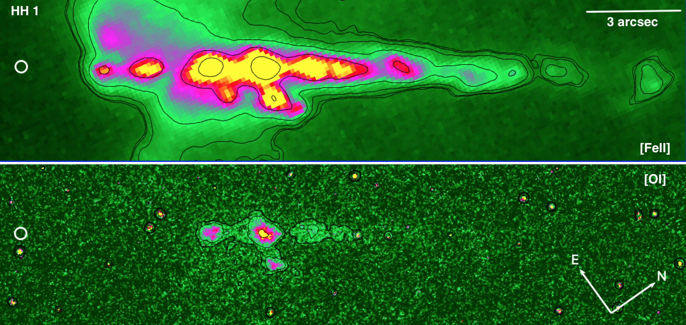
Figure 18: The HH 1 jet imaged in [Fe II] 1.25$\mu$m (top) and [O I] 6300Åemission (bottom). These images are not continuum-subtracted. [Fe II] contours are 0.1, 0.11, 0.13, 0.22, 0.57 and 2 $\times$10^-18 erg s^-1 cm^-2 Å^-1 pixel^-1. [O I] contours are 0.5, 0.53, 0.85 and 4 $\times$10^-19 erg s^-1 cm^-2 Å^-1 pixel^-1.

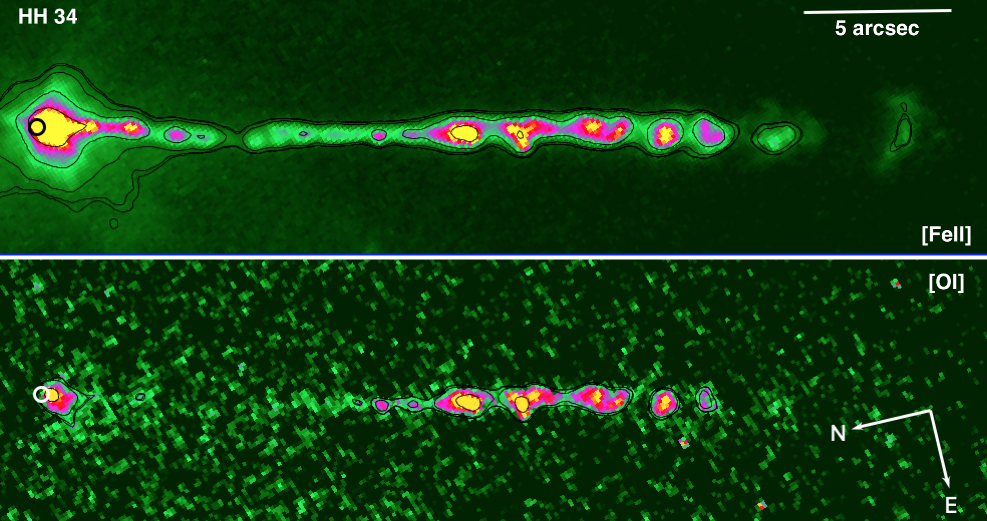
Figure 19: Same as Figure 18. [Fe II] contours are 0.9, 0.95, 1.2, 2.5 and 10 $\times$10^-19 erg s^-1 cm^-2 Å^-1 pixel^-1. [O I] contours are 2, 2.05, 2.5 and 7 $\times$10^-20 erg s^-1 cm^-2 Å^-1 pixel^-1.

Figure 20: Same as Figure 18.[Fe II] contours are 0.08, 0.09, 0.1, 0.2, 0.56 and 2 $\times$10^-18 erg s^-1 cm^-2 Å^-1 pixel^-1. [O I] contours are 4, 5.2, 6.5, 7.7 and 9 $\times$10^-20 erg s^-1 cm^-2 Å^-1 pixel^-1.

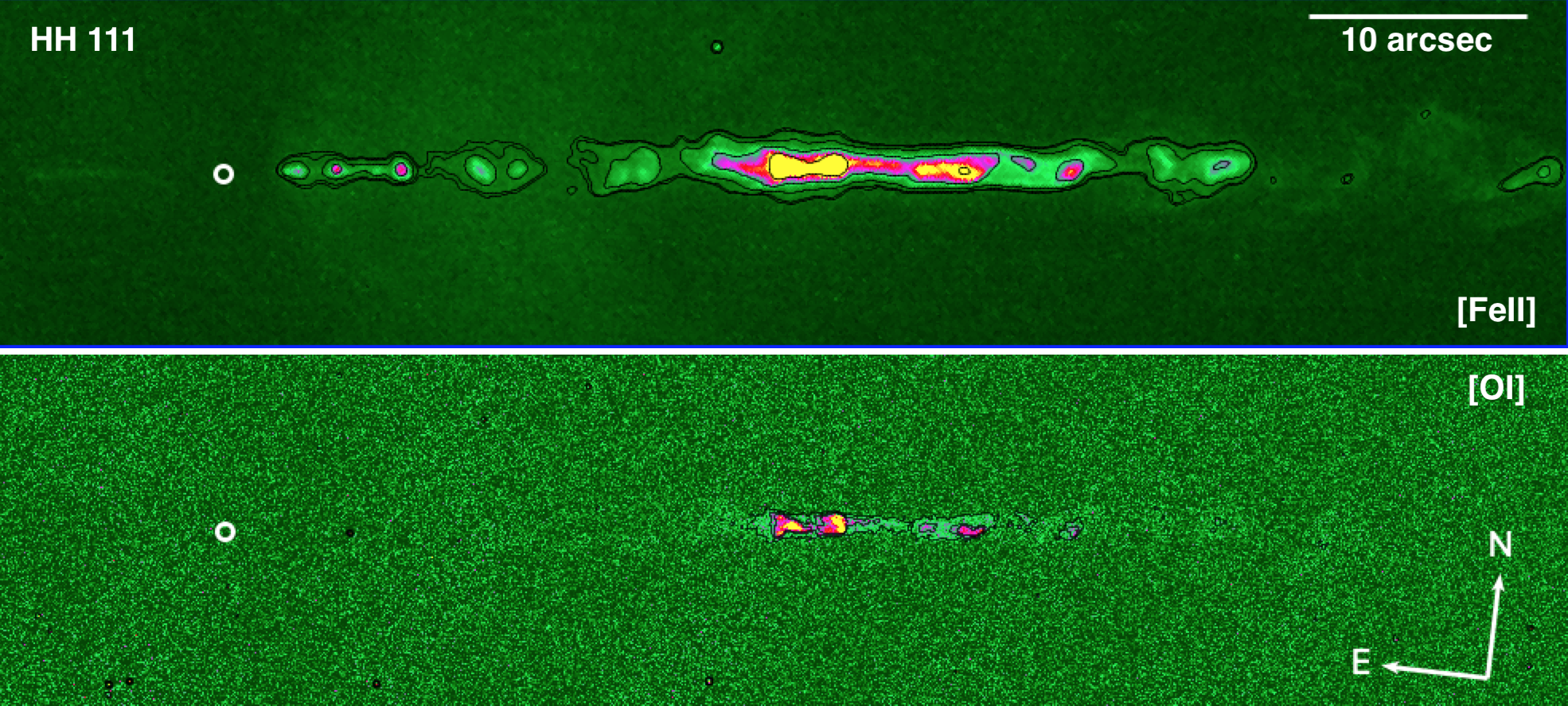
Figure 21: Same as Figure 18. [Fe II] contours are 0.6, 0.65, 0.9, 2.2 and 10 $\times$10^-19 erg s^-1 cm^-2 Å^-1 pixel^-1. [O I] contours are 0.3, 0.65 and 1 $\times$10^-19 erg s^-1 cm^-2 Å^-1 pixel^-1.

Appendix B [O I] 6300 Å/[Fe II] 1.64 $\mu$m line ratio maps

Figure 22 shows the images of the [O I] 6300 Å/[Fe II] 1.64 $\mu$m line ratio in the four observed objects. The images were obtained using the non-continuum subtracted images, to avoid introducing additional noise to the [O I] images. We masked the ratio images to include only the ratio in the jet and bowshocks where both [O I] and [Fe II] emission are above the set RMS threshold. HH 1, HH 34 and HH 111 were masked so that only emission above 2 $\times$ RMS are present. HH 46 was masked at 1 $\times$ RMS. The ratios appear rather uniform in the different regions. In bow shock regions, e.g. HH 1/2 and HH 46/47, the observed ratio is typically between 0.5 and 2, while along the jets it is lower, with values of $\sim$ 0.2 - 0.3. This is mainly an extinction effect: if we correct the observed values for the extinction derived from the [Fe II] line ratio, we find that the [O I] 6300 Å/[Fe II] 1.64 $\mu$m ratio is consistent with what is expected from a gas with a temperature between 6000-10000 K, and electron density between 10³-10⁴ cm^-3, as estimated in the literature for these jets (e.g Giannini et al., 2015; Nisini et al., 2005, 2016). Spatial gradients of the ratio are also observed within the individual structures (e.g. in the HH 1 and HH 47 bow shocks) and are likely due to gradients in temperature in the post-shock regions.

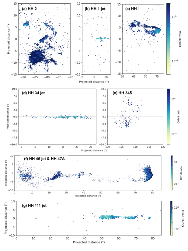
Figure 22: [O I] 6300 Å/[Fe II] 1.64 $\mu$m line ratio maps for various parts of each of our sources. Panels (a)-(c) show the [O I]/[Fe II] ratio for the HH 2 bowshock, HH 1 inner jet region and the HH 1 bowshock, respectively. Panels (d) and (e) show the [O I]/[Fe II] ratio for the HH 34 inner jet region and the HH 34S bowshock, respectively. Panel (f) shows the ratio for the HH 46 jet and bowshock HH 47A and panel (g) is the inner region of the HH 111 jet. All figures are masked above where the [O I] emission is above 2 $\times$ RMS, except for HH 46 (panel (f)) where it is masked above 1 $\times$ RMS.

Appendix C Tables of Jet Tangential Velocities

Table 6: Proper motions and tangential velocities for the knots in the HH 34 jet compared to velocities reported by Raga et al. (2012). Velocities are calculated assuming d=383 pc and Raga et al. (2012) values were corrected to d=383 pc.

Knot	z	$\Delta$z	v2019	v2012
	(”)	(”)	(km s-1)	(km s-1)
1	1.806	-	-	-
2	3.195	1.076	173.4	171 (1)
3	4.733	0.918	148.0	202 (2)
4	5.651	0.833	134.3	171 (3)
5	7.437	1.057	170.4	175 (4)
6	8.305	1.096	176.7	164 (5)
7	9.099	0.919	148.2	163 (6)
8	10.141	0.936	150.9	141 (7)
9	11.604	0.937	151.1	162 (8)
10	12.722	0.935	150.7	165 (9)
11	14.359	1.005	162.0	156 (10)
12	14.730	0.800	129.0	156 (11)
13	16.493	0.791	127.5	142 (12)
14	16.788	0.815	131.4
15	18.873	0.878	141.5	148 (13)
16	19.767	0.856	138.0	148 (14)
17	21.454	0.940	151.5	148 (15)
18	22.743	0.918	148.0	138 (16)
19	23.140	0.802	129.3
20	25.049	0.835	134.6	133 (17)
21	29.515	0.793	127.8	143 (18)

Table 7: Proper motions and tangential velocities for the knots in the HH 46 jet compared to velocities reported by Hartigan et al. (2005), assuming a distance of 450 pc.

Knot	z	$\Delta$z	v2019	v2005
	(”)	(”)	(km s-1)	(km s-1)
1	19.3	1.165	220.9	192 (Js2)
2	22.2	1.154	218.9	246 (Js3)
3	24.1	1.145	217.2	207 (Js6)
4	25.2	1.229	233.1	200 (Js7)
5	30.6	1.145	217.2	231 (Js10)
6	37.2	1.196	226.8	236 (Js12)
7	39.2	1.346	255.3	244 (Js13)
8	43.6	0.860	163.1	230 (Js14)
9	46.2	1.192	226.1	248 (Js15)
10	49.3	1.598	303.1	251 (Js17)
11	54.3	1.598	303.1	252 (Js18)
12	60.2	1.734	328.9	252 (Js19)
13	68.3	1.391	263.8	283 (Js20)
14	74.7	1.554	294.8	299 (As1)
15	78.9	1.107	209.9	236 (As18)

Table 8: Proper motions and tangential velocities for the knots in the HH 111 jet compared to velocities reported by Hartigan et al. (2001). Velocities are calculated assuming d=400pc and Hartigan et al. (2001) values were corrected to d=400pc.

Knot	z	$\Delta$z	v2019	v2001
	(”)	(”)	(km s-1)	(km s-1)
E	26.2	2.758	256.4	256 (E3)
				284 (E2)
F	28.3	2.239	208.1	259 (F2)
				217 (F1)
G	32.2	2.352	218.7	249 (G1)
H	34.1	2.095	194.8	231 (H)
I	36.9	2.151	199.9	211 (I2)
				228 (I1)
J	38.9	1.935	179.9	229 (J)
K	43.3	2.621	243.7	247 (K)
L	46.1	2.476	230.2	192 (L)

Appendix D Contamination of various [Fe II] lines in the WFC3 narrow band filters

The WFC3 narrow band filters used in this study cover several emission lines whose contribution can contaminate the measurement of the [Fe II] 1.25, 1.64$\mu$m line flux, in particular when considering continuum-subtracted images. Hydrogen lines of the Brackett series, like the Br 11 at 1.681$\mu$m and Br 12 at 1.641$\mu$m fall into the F167N and F164N filter band widths, respectively. However, their emission in the investigated jets is negligible, as testified by IR spectroscopy of some of them (i.e. Nisini et al., 2005, Podio et al. 2010). More relevant is the emission of the other numerous [Fe II] lines, whose relative intensity is a function of the electron density (Nisini et al., 2002).

Table 9 lists the [Fe II] lines that are covered by the filters and their relative intensity with respect to the 1.64$\mu$m line for temperature $T_{e}$ = 10 000 K and density $n_{e}$ = 10³ and 10⁴ cm^-3. At low density, the contribution of these lines within each filter is a few % and can be thus considered negligible. However, at higher density the contribution of some of the lines falling into the continuum filters is up to 20%. Consequently, the flux measured in the continuum-subtracted images can be underestimated by up to this factor. This is the case in the inner and denser jet region, where densities as large as 5 10⁴ cm^-3 have been estimated (Nisini et al., 2005, Podio et al., 2006, Nisini et al., 2016). We note, however, that the contamination of weaker lines in the F130N filter is comparable to that of the F167N filter, being in both cases a similar fraction of the 1.25 and 1.64 $\mu$m emission. Consequently, when the line ratio is estimated from the ratio of the relative continuum-subtracted images, the uncertainty introduced by the contaminating lines is not larger than 5% at most.

Table 9: [Fe II] lines falling within the HST filters

Line	$\lambda$	$I(n_{e}=10^{3}cm^{-3})$	$I(n_{e}=10^{4}cm^{-3})$
F126N, $\lambda_{o}$ = 1258.5 nm, $\Delta\lambda$ = 15.2 nm
Fe II a4D7/2-a6D9/2	1.257 $\mu$m	1	1
Fe II a4D1/2-a6D3/2	1.252 $\mu$m	0.003	0.01
F130N, $\lambda_{o}$ = 1300.0 nm, $\Delta\lambda$ = 15.6 nm
Fe II a4D5/2-a6D5/2	1.2946 $\mu$m	0.05	0.17
Fe II a4D3/2-a6D1/2	1.2981 $\mu$m	0.01	0.04
F164N, $\lambda_{o}$ = 1640.4 nm, $\Delta\lambda$ = 20.9 nm		0.73	0.73
Fe II a4D7/2-a4F9/2	1.6440 $\mu$m
F167N, $\lambda_{o}$ = 1664.2 nm, $\Delta\lambda$ = 21.0 nm
Fe II a4D1/2-a4F5/2	1.6642 $\mu$m	0.013	0.05
Fe II a4D5/2-a4F7/2	1.6773 $\mu$m	0.04	0.1

References

- Agra-Amboage et al. (2011) Agra-Amboage, V., Dougados, C., Cabrit, S., & Reunanen, J. 2011, Astronomy & Astrophysics, 532, A59, doi: 10.1051/0004-6361/201015886
- Anglada et al. (2007) Anglada, G., López, R., Estalella, R., et al. 2007, AJ, 133, 2799, doi: 10.1086/517493
- Antoniucci, S. et al. (2014) Antoniucci, S., La Camera, A., Nisini, B., et al. 2014, A&A, 566, A129, doi: 10.1051/0004-6361/201423944
- Arce et al. (2013) Arce, H. G., Mardones, D., Corder, S. A., et al. 2013, ApJ, 774, 39, doi: 10.1088/0004-637X/774/1/39
- Bacciotti et al. (2002) Bacciotti, F., Ray, T. P., Mundt, R., Eislöffel, J., & Solf, J. 2002, ApJ, 576, 222, doi: 10.1086/341725
- Bally et al. (2002) Bally, J., Heathcote, S., Reipurth, B., et al. 2002, The Astronomical Journal, 123, 2627
- Binette et al. (1999) Binette, L., Cabrit, S., Raga, A., & Cantó, J. 1999, A&A, 346, 260
- Cardelli et al. (1989) Cardelli, J. A., Clayton, G. C., & Mathis, J. S. 1989, ApJ, 345, 245, doi: 10.1086/167900
- Chrysostomou et al. (2008) Chrysostomou, A., Bacciotti, F., Nisini, B., et al. 2008, A&A, 482, 575, doi: 10.1051/0004-6361:20078494
- Coffey et al. (2004) Coffey, D., Bacciotti, F., Woitas, J., Ray, T. P., & Eislöffel, J. 2004, ApJ, 604, 758, doi: 10.1086/382019
- Coppin et al. (1998) Coppin, K. E. K., Davis, C. J., & Micono, M. 1998, MNRAS, 301, L10, doi: 10.1046/j.1365-8711.1998.02146.x
- Davis et al. (2000) Davis, C. J., Smith, M. D., & Eislöffel, J. 2000, MNRAS, 318, 747, doi: 10.1046/j.1365-8711.2000.03766.x
- Davis et al. (2003) Davis, C. J., Whelan, E., Ray, T. P., & Chrysostomou, A. 2003, A&A, 397, 693, doi: 10.1051/0004-6361:20021545
- Davis et al. (2011) Davis, C. J., Cervantes, B., Nisini, B., et al. 2011, A&A, 528, A3, doi: 10.1051/0004-6361/201015897
- Eislöffel et al. (1994) Eislöffel, J., Davis, C. J., Ray, T. P., & Mundt, R. 1994, ApJ, 422, L91, doi: 10.1086/187220
- Eislöffel & Mundt (1992) Eislöffel, J., & Mundt, R. 1992, Astronomy and Astrophysics, 263, 292
- Eislöffel & Mundt (1994) Eislöffel, J., & Mundt, R. 1994, A&A, 284, 530
- Eislöffel et al. (1996) Eislöffel, J., Smith, M. D., Davis, C. J., & Ray, T. P. 1996, AJ, 112, 2086, doi: 10.1086/118165
- Estalella et al. (2012) Estalella, R., López, R., Anglada, G., et al. 2012, AJ, 144, 61, doi: 10.1088/0004-6256/144/2/61
- Ferreira et al. (2006) Ferreira, J., Dougados, C., & Cabrit, S. 2006, A&A, 453, 785, doi: 10.1051/0004-6361:20054231
- Frank et al. (2014) Frank, A., Ray, T., Cabrit, S., et al. 2014, Protostars and planets VI, 451
- Garcia Lopez et al. (2010) Garcia Lopez, R., Nisini, B., Eislöffel, J., et al. 2010, A&A, 511, A5, doi: 10.1051/0004-6361/200913304
- Giannini et al. (2015) Giannini, T., Antoniucci, S., Nisini, B., Bacciotti, F., & Podio, L. 2015. https://arxiv.org/abs/1510.06880
- Giannini et al. (2015) Giannini, T., Antoniucci, S., Nisini, B., et al. 2015, ApJ, 798, 33, doi: 10.1088/0004-637X/798/1/33
- Großschedl et al. (2018) Großschedl, J. E., Alves, J., Meingast, S., et al. 2018, A&A, 619, A106, doi: 10.1051/0004-6361/201833901
- Gueth et al. (1996) Gueth, F., Guilloteau, S., & Bachiller, R. 1996, A&A, 307, 891
- Hartigan et al. (2004) Hartigan, P., Edwards, S., & Pierson, R. 2004, ApJ, 609, 261, doi: 10.1086/386317
- Hartigan et al. (2005) Hartigan, P., Heathcote, S., Morse, J. A., Reipurth, B., & Bally, J. 2005, AJ, 130, 2197, doi: 10.1086/491673
- Hartigan et al. (2001) Hartigan, P., Morse, J. A., Reipurth, B., Heathcote, S., & Bally, J. 2001, ApJ, 559, L157, doi: 10.1086/323976
- Hartigan et al. (2011) Hartigan, P., Frank, A., Foster, J. M., et al. 2011, ApJ, 736, 29, doi: 10.1088/0004-637X/736/1/29
- Lee et al. (2017) Lee, C.-F., Ho, P. T. P., Li, Z.-Y., et al. 2017, Nature Astronomy, 1, 0152, doi: 10.1038/s41550-017-0152
- Lee et al. (2016) Lee, C.-F., Hwang, H.-C., & Li, Z.-Y. 2016, ApJ, 826, 213, doi: 10.3847/0004-637X/826/2/213
- Lee et al. (2020) Lee, C.-F., Li, Z.-Y., & Turner, N. J. 2020, Nature Astronomy, 4, 142, doi: 10.1038/s41550-019-0905-x
- Masciadri et al. (2002) Masciadri, E., de Gouveia Dal Pino, E. M., Raga, A. C., & Noriega-Crespo, A. 2002, ApJ, 580, 950, doi: 10.1086/343797
- Masciadri & Raga (2002) Masciadri, E., & Raga, A. 2002, The Astrophysical Journal, 568, 733
- Maurri et al. (2014) Maurri, L., Bacciotti, F., Podio, L., et al. 2014, A&A, 565, A110, doi: 10.1051/0004-6361/201117510
- Nisini et al. (2005) Nisini, B., Bacciotti, F., Giannini, T., et al. 2005, A&A, 441, 159, doi: 10.1051/0004-6361:20053097
- Nisini et al. (2002) Nisini, B., Caratti o Garatti, A., Giannini, T., & Lorenzetti, D. 2002, A&A, 393, 1035, doi: 10.1051/0004-6361:20021062
- Nisini et al. (2016) Nisini, B., Giannini, T., Antoniucci, S., et al. 2016, A&A, 595, A76, doi: 10.1051/0004-6361/201628853
- Noriega-Crespo et al. (2020) Noriega-Crespo, A., Raga, A. C., Lora, V., & Rodríguez-Ramírez, J. C. 2020, Rev. Mexicana Astron. Astrofis., 56, 29, doi: 10.22201/ia.01851101p.2020.56.01.05