Stochastic Whitening Batch Normalization

Abstract

Batch Normalization (BN) is a popular technique for training Deep Neural Networks. BN uses scaling and shifting to normalize activations of mini-batches to accelerate convergence and improve generalization. The recently proposed Iterative Normalization (IterNorm) method improves these properties by whitening the activations iteratively using Newton’s method. However, since Newton’s method initializes the whitening matrix independently at each training step, no information is shared between consecutive steps. In this work, instead of exact computation of whitening matrix at each time step, we estimate it gradually during training in an online fashion, using our proposed Stochastic Whitening Batch Normalization (SWBN) algorithm. We show that while SWBN improves the convergence rate and generalization of DNNs, its computational overhead is less than that of IterNorm. Due to the high efficiency of the proposed method, it can be easily employed in most DNN architectures with a large number of layers. We provide comprehensive experiments and comparisons between BN, IterNorm, and SWBN layers to demonstrate the effectiveness of the proposed technique in conventional (many-shot) image classification and few-shot classification tasks.

1 Introduction

Gradient descent-based methods are the de-facto training algorithms for DNN, and mini-batch Stochastic Gradient Decent (SGD) has become the most popular first-order optimization algorithm. In mini-batch SGD, instead of computing the gradients for the entire training set as in batch gradient descent, or based on one training sample as in conventional SGD, the gradients are computed based on a small random subset of the training set called mini-batch. The stochastic nature of mini-batch SGD helps a DNN find better local optima or even the global optima than batch gradient descent. We use SGD to refer to mini-batch SGD in the rest of the paper.

Due to the change in the distribution of the inputs of DNN layers at each training step, the network experiences Internal Covariate Shift (ICS) as defined in the seminal work of  [17]. ICS affects the input statistics of the subsequent layers, and as a result, it degrades the training efficiency.

Eliminating the effect of ICS can accelerate the training of DNN by helping the gradient flow through the network, stabilizing the distributions of the activations, and enabling the use of a larger learning rate. To alleviate these effects, BN has been proposed in [17].

Recent studies have shown that whitening (decorrelating) the activations can further reduce the training time and improve the generalization [8, 24, 15]. However, when dealing with high-dimensional data, the requirement of eigen-decomposition [8, 24], Singular Value Decomposition (SVD), or Newton’s iteration [15] for computing whitening matrices has been the bottleneck of these methods.

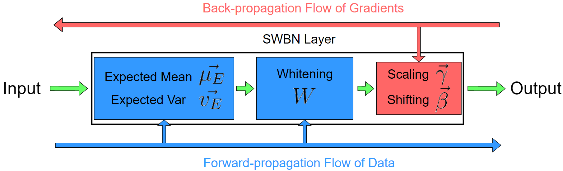
Figure 1: The SWBN diagram shows how whitening parameters and task parameters inside an SWBN layer are updated in a decoupled way. Whitening parameters (in blue rectangles) are updated only in the forward phase, and are fixed in the backward phase. Task parameters (in red rectangles) are fixed in the forward phase, and are updated only in the backward phase.

In this paper, we propose a method called SWBN, which gradually learns whitening matrices separately in each layer during training. The proposed method eliminates the need for expensive matrix decomposition and inversion for whitening data as SWBN learns the whitening matrix in an online fashion. Our formulation clearly shows the computational advantage of SWBN to other whitening techniques applied in DNNs, such as [8], [15] and [14].

In Section 2, we review the related works on normalization and whitening techniques for DNN. In Section 3, we derive and discuss the SWBN algorithm. In Section 4, we present extensive experimental results to show the effectiveness of the proposed method for different network architectures and datasets. In summary, the key advantages of the proposed method are as follows:

• SWBN is designed to be a drop-in replacement for BN. It decouples the learning process of whitening matrices from the back-propagation algorithm. Thus there is no need to modify the network architecture, task loss, or the optimization algorithm to enable whitening.

• SWBN takes advantages of both BN and whitening to improve convergence rate and generalization performance of DNN models with small computational overhead.

• There are a few whitening approaches that aim to serve as drop-in replacements for BN layers. However, they can only replace a small number of BN layers in a DNN with their whitening layers due to the computational burden. In contrast, SWBN learns whitening matrices without expensive matrix decomposition or matrix inversion operations, enabling SWBN layers to replace a large number of BN layers.

2 Related Works

Activation normalization is known to be a very effective technique in speeding up the training of DNNs [25]. A straightforward solution is to center the input mean to zero, and use nonlinear activation functions that range from -1 to 1 [22]. Although this method limits the activation values, activation distribution may still largely vary during the training, as caused by the change in the parameters of the previous layers known as ICS.

To alleviate ICS, BN was proposed as a technique that employs the mean and variance of the mini-batch to normalize the activations [17]. At training time, this technique stabilizes the distributions of the activations and allows the use of larger learning rates. BN, however, may not work well with small mini-batches, because mean and variance estimates are less accurate. To improve the estimation accuracy for small mini-batches, other variants have been proposed, such as Batch Renormalization [16], Weight Normalization [26], Layer Normalization [1], Group Normalization [32], Online Normalization [5], PowerNorm [27], and Streaming Normalization [23], etc.

Whitening (decorrelating) the activations may further improve the training time and generalization of DNN models. This usually happens as a result of improving the conditioning of the input covariance matrix, which leads to better conditioning of the Hessian matrix or Fisher information matrix of network parameters. One way to whiten activations is to add regularization terms to the task loss. Cogswell et al. [6] have proposed a regularizer, DeCov, that adds decorrelation loss to the task loss function, which encourages decorrelation between activations and non-redundant representations in DNNs. An extended version of DeCov based on group-based decorrelation loss has been proposed in [34]. In [35], spectral norm regularization is proposed. It designs a penalty term added to the task loss function, which regularizes parameter matrices by the approximated largest singular values and their corresponding singular vectors via the Power Iteration method. Although these methods are shown to improve network generalization, they introduce extra hyper-parameter to merge the decorrelation regularizer with the task loss.

Some approaches do not introduce any extra term to the task loss. Natural neural networks [8] and generalized whitened neural networks [24] propose two types of Zero-phase Component Analysis (ZCA)-based whitening layers to improve the conditioning of the Fisher information matrix of a DNN. To avoid the high cost of eigenvalue decomposition that is required to compute the whitening matrix, both methods amortize the cost over multiple consecutive updates, by performing the whitening step only at every certain number of iterations. Similarly, Decorrelated Batch Normalization (DBN) [14] directly whitens the activations by eigenvalue decomposition of the sample covariance matrix computed over each mini-batch, but its usage in a large DNN is limited due to its high computational cost. Further, [31] proposes back-propagation friendly eigen-decomposition to whiten the activations by combining the Power Iteration method and the truncated SVD. IterNorm [15], as an improved version of DBN, uses Newton’s method to compute the square root inverse of the covariance matrix, iteratively. Although Newton’s method improves the whitening efficiency, IterNorm still has the following drawbacks: First, ZCA whitening is used for each mini-batch independently. In other words, at each training step, the exact whitening matrix is computed specifically for the current mini-batch. As a result, the information of this whitening matrix does not carry over to the computation of the whitening matrix at the next step. Second, because Newton’s method requires multiple iterations of matrix multiplication, applying IterNorm to all the layers of a very deep neural network is computationally inefficient.

3 Stochastic Whitening Batch Normalization

In this section, we first review the whitening techniques and explain the issues that arise when these techniques are employed directly in the training of DNN models. Later, we introduce our stochastic whitening batch normalization algorithm and provide explanations and complexity analysis of how and why SWBN works.

3.1 Whitening Transformation

A random vector $\vec{z}\in\mathbb{R}^{d}$, with zero mean, is said to be white if the expectation of the covariance of $\vec{z}$ satisfies $E[\vec{z}\vec{z}^{T}]=I_{d}$, where $I_{d}$ is an identity matrix. Therefore, elements of $\vec{z}$ have unit variance and are mutually uncorrelated. Whitening is a process that transforms a zero-mean random vector $\vec{x}\in\mathbb{R}^{d}$ into $\vec{z}$ by a linear transformation. Existing methods for data whitening are to search for a transformation matrix $W\in\mathbb{R}^{d\times d}$, such that $\vec{z}=W\vec{x}$ [19]. Principal Component Analysis (PCA) whitening and ZCA whitening algorithms are two commonly used methods. Both of these algorithms require the covariance matrix $\Sigma_{\vec{x}}=E[\vec{x}\vec{x}^{T}]$, and its decomposition via eigenvalue decomposition, or Cholesky decomposition on its inverse matrix $\Sigma_{\vec{x}}^{-1}$.

The eigenvalue decomposition decomposes the covariance matrix as $\Sigma_{\vec{x}}=UDU^{T}$, where $U$ is an orthogonal matrix and $D$ is a diagonal matrix with eigenvalues of the covariance matrix on its diagonal. In the case of Cholesky decomposition, we have $\Sigma_{\vec{x}}^{-1}=LL^{T}$, where $L$ is a lower triangular matrix with positive diagonal values. In practice, the sample covariance matrix $\hat{\Sigma}_{\vec{x}}$ is used. In this work, we only consider PCA and ZCA whitening algorithms. In PCA whitening, the transformation matrix $W$ is of the form $W=D^{-1/2}U^{T}$, and in ZCA whitening $W$ is of the form $W=UD^{-1/2}U^{T}$. It is worth mentioning that left-multiplying any orthogonal matrix to the PCA whitening matrix $W$ forms a new whitening matrix [19]. The ZCA whitening matrix is the only whitening matrix that is symmetric.

More details of these whitening algorithms are included in [2], [9], [18], and [19].

3.2 Introduction to SWBN

The computational cost of whitening matrices usually becomes the bottleneck when applying any of the above-mentioned whitening algorithms to train a DNN, especially for networks with millions or billions of parameters. One important question to answer is whether the complete whitening process is necessary at each training step. Because of ICS, a whitening matrix computed at one step could be very different from the one computed at the next step, making the full computation of the whitening matrix at the previous step a waste. Therefore, it will be ideal if the whitening algorithm can reduce the computational cost via gradually whitening the data over training iterations.

In this work, we introduce SWBN, a stochastic algorithm that gradually learns whitening matrices and whitens activations simultaneously. SWBN whitens the activations by stochastically minimizing a whitening loss with respect to an internal matrix. A whitening loss is a function of the covariance matrix. The internal matrix keeps track of the changes of the input distribution through the loss minimization, and eventually becomes a whitening matrix. However, unlike DeCov, spectral norm, or any other methods involving modification of the loss functions, in SWBN, the whitening loss is decoupled from the task loss. Decoupling them not only reduces the chance of divergence at training time but also speeds up convergence. Also, as shown in [15], although fully whitening the activations helps accelerate convergence, partial whitening on each mini-batch may yield better generalization due to the noise introduced from partial whitening. In addition, different from DBN or IterNorm that completely whiten activations at each step, an SWBN layer uses its internal matrix to “slightly” whiten the activations with respect to a predefined whitening loss before they are fed into the next layer. As training continues, the matrix gets closer to the final whitening matrix, and the output of an SWBN layer becomes whiter. We discuss two whitening criteria in the next subsection.

3.3 Whitening Criteria

We define the whitening criterion as the whitening loss function, which is a measure of distance between a covariance matrix and the identity matrix.

Definition 1.

A whitening criterion for a positive semi-definite matrix $\Sigma$ is a function $C:\mathbb{S}^{n}_{+}\mapsto\mathbb{R}^{+}\cup\{0\}$ that maps $\Sigma$ to a non-negative real number which quantifies the dissimilarity between $\Sigma$ and the identity matrix $I$. $\mathbb{S}^{n}_{+}$ represents a set of positive semi-definite matrices of size $n\times n$.

With this definition, we can define a whitening matrix under a criterion $C$ for a random vector $\vec{x}$.

Definition 2.

Let $\vec{x}\in\mathbb{R}^{d}$ be a zero-mean $d$-dimensional random vector and $\Sigma_{\vec{x}}=E[\vec{x}\vec{x}^{T}]$. A matrix $W^{*}$ is called a whitening matrix under a criterion C, or C-whitening matrix, of $\vec{x}$, $W$ satisfies:

$$W^{*}=\arg\min_{W}\,\,C(\Sigma_{\vec{y}})=\arg\min_{W}C(W\Sigma_{\vec{x}}W^{T})$$

where $\vec{y}=W\vec{x}$, and $\Sigma_{\vec{y}}=E[\vec{y}\vec{y}^{T}]=WE[\vec{x}\vec{x}^{T}]W^{T}$.

In this work, we consider the following two whitening criteria derived by Kullback–Leibler (KL) divergence and Frobenius norm:

$$C_{\text{KL}}(W\Sigma_{\vec{x}}W^{T}) =\frac{1}{2}(tr(W\Sigma_{\vec{x}}W^{T})-\ln\det(W\Sigma_{\vec{x}}W^{T})-d)$$ (1)

$$C_{\text{Fro}}(W\Sigma_{\vec{x}}W^{T}) =\frac{1}{2}||I-W\Sigma_{\vec{x}}W^{T}||_{\text{Fro}}$$ (2)

It is obvious that both criteria reach their minimum values of $0$ if $W\Sigma_{\vec{x}}W^{T}=I_{d}$. The first criterion is derived from KL divergence based on the assumption of having two zero-mean Gaussian distributions with covariance matrices equal to $\Sigma_{\vec{y}}$ and $I_{d}$. The second criterion directly computes the Frobenius norm of the difference between the identity matrix $I_{d}$ and the sample covariance matrix. Unlike $C_{KL}$, $C_{Fro}$ has no assumptions on the probability distribution. These two criteria are the core of the proposed SWBN algorithm. More details can be found in Appendix B.

3.4 Update Rules for SWBN Layer

Assume $\vec{x}$ is an input vector to a hidden layer of a DNN model. We find the $C$-whitening matrix $W$ of each layer by minimizing the whitening criterion using SGD. We update $W$ by $W\leftarrow W-\alpha\Delta W$, where $\alpha$ is the step size and $\Delta W$ is the update matrix. The update rules with respect to the criteria in Eq. ($1$) and Eq. ($2$) mentioned above are:

$$\Delta W=\left\{\begin{matrix}(W\hat{\Sigma}_{\vec{x}}W^{T}-I_{d})W,\quad\hfill{\text{for $C_{\text{KL}}$}},\\ \frac{(W\hat{\Sigma}_{\vec{x}}W^{T}-I_{d})W\hat{\Sigma}_{\vec{x}}}{||I_{d}-W\hat{\Sigma}_{\vec{x}}W^{T}||_{Fro}},\quad\hfill{\text{for $C_{\text{Fro}}$}},\end{matrix}\right.$$ (3)

where $\hat{\Sigma}_{\vec{x}}$ is the sample covariance matrix.

Cardoso et al. [4] shows that optimizing $W$ to be a minimizer of $C_{\text{KL}}$ by its update rule in Eq. (3) results in a whitening matrix. To our knowledge, this is the first time that the update rule of $C_{KL}$ is applied in a mini-batch SGD setting for training DNNs. The proposed update rule of $C_{Fro}$ is not only less sensitive to the whitening step size and the batch size, but also shows better performance on few-shot classification, based on the experimental results in Section 4. Unlike the update rule of $C_{\text{Fro}}$, the update rule of $C_{\text{KL}}$ is derived by relative gradients. The derivation of these update rules and the detailed discussion are given in Appendix B.

3.5 SWBN Algorithm

Input :  Input batch $X\in\mathbb{R}^{d\times n}=[\vec{x}_{1},\cdots,\vec{x}_{n}]$

Output :  Processed data $\hat{X}\in\mathbb{R}^{d\times n}$

Initialization:

Whitening parameters: $W=I_{d}$;

Task parameters: $\vec{\gamma}$, $\vec{\beta}\in\mathbb{R}^{d}$;

Hyperparameters: tolerance $\epsilon=10^{-8}$, moving average momentum $\eta=0.95$, step size $\alpha$;

Criterion: $C=C_{\text{KL}}$ or $C_{\text{Fro}}$;

Expected mean and variance: $\vec{\mu}_{E}=\vec{0}$, $\vec{v}_{E}=\vec{1}$.

1. Calculate batch mean: $\vec{\mu}\leftarrow\frac{1}{n}\Sigma_{i=1}^{n}\vec{x}_{i}$

2. Calculate batch variance: $\vec{v}\leftarrow\frac{1}{n-1}\Sigma_{i=1}^{n}(\vec{x}_{i}-\vec{\mu})\odot(\vec{x}_{i}-\vec{\mu})$

3. Update the expected mean: $\vec{\mu}_{E}\leftarrow\eta\vec{\mu}_{E}+(1-\eta)\vec{\mu}$

4. Update the expected variance: $\vec{v}_{E}\leftarrow\eta\vec{v}_{E}+(1-\eta)\vec{v}$

5. Standardize data: $X^{S}\leftarrow\Lambda^{-\frac{1}{2}}(X-\vec{\mu}\vec{1}_{n}^{T})$, where $\Lambda\leftarrow diag(\vec{v})+\epsilon I_{d}$

6. Calculate sample covariance matrix: $\hat{\Sigma}_{B}\leftarrow\frac{1}{n}X^{S}(X^{S})^{T}$

7. Compute and update matrix from Eq. (3): $W\leftarrow W-\alpha\Delta W$

8. Enforce symmetry constraint: $W\leftarrow 0.5(W+W^{T})$

9. Multiply $W$ to standardized data: $X^{W}\leftarrow WX^{S}$

10. Compute output: $\hat{X}\leftarrow X^{W}\odot(\vec{\gamma}\vec{1}^{T}_{n})+(\vec{\beta}\vec{1}^{T}_{n})$

Algorithm 1 Forward Propagation of SWBN Layers at Training Phase

Input :  Gradients of task loss $L$ w.r.t output $\frac{\partial L}{\partial\hat{X}}\in\mathbb{R}^{d\times n}$

Intermediate data from Algorithm 1, $X^{S}$, $X^{W}$, $\vec{\mu}$, $\vec{v}$

Whitening matrix from Algorithm 1, $W$

Output :  Gradients w.r.t. $X$, $\vec{\gamma}$, $\vec{\beta}$ i.e. $\frac{\partial L}{\partial X}\in\mathbb{R}^{d\times n}$, $\frac{\partial L}{\partial\vec{\gamma}}\in\mathbb{R}^{d}$, $\frac{\partial L}{\partial\vec{\beta}}\in\mathbb{R}^{d}$

Initialization: $\frac{\partial L}{\partial X}\leftarrow\mathbf{0}_{d\times n}$, $\frac{\partial L}{\partial\vec{\gamma}}\leftarrow\vec{0}_{d}$, $\frac{\partial L}{\partial\vec{\beta}}\leftarrow\vec{0}_{d}$

for $k=1,\dots,d$ do

       $[\frac{\partial L}{\partial\vec{\gamma}}]_{k}\leftarrow\Sigma_{j=1}^{n}\frac{\partial L}{\partial\hat{X}_{kj}}X^{W}_{kj}$

       $[\frac{\partial L}{\partial\vec{\beta}}]_{k}\leftarrow\Sigma_{j=1}^{n}\frac{\partial L}{\partial\hat{X}_{kj}}$

       for $l=1,\dots,n$ do

             $\frac{\partial X^{S}_{kl}}{\partial v_{k}}\leftarrow-\frac{1}{2}(X^{S}_{kl}-\mu_{k})(v_{k}+\epsilon)^{-\frac{3}{2}}$

             $\frac{\partial X^{S}_{kl}}{\partial\mu_{k}}\leftarrow-\frac{1}{\sqrt{v_{k}+\epsilon}}$

             $\frac{\partial v_{k}}{\partial X_{kl}}\leftarrow\frac{2}{n-1}(X_{kl}-\mu_{k})$

             $\frac{\partial\mu_{k}}{\partial X_{kl}}\leftarrow\frac{1}{n}$

             $\frac{\partial X^{S}_{kl}}{\partial X_{kl}}\leftarrow\frac{1}{\sqrt{v_{k}+\epsilon}}+\frac{\partial X^{S}_{kl}}{\partial v_{k}}\frac{\partial v_{k}}{\partial X_{kl}}+\frac{\partial X^{S}_{kl}}{\partial\mu_{k}}\frac{\partial\mu_{k}}{\partial X_{kl}}$

             $[\frac{\partial L}{\partial X}]_{kl}\leftarrow\frac{\partial X^{S}_{kl}}{\partial X_{kl}}\Sigma_{i=1}^{d}\gamma_{i}W_{ik}\frac{\partial L}{\partial\hat{X}_{il}}$

       end for

      

end for

Algorithm 2 Back-propagation of SWBN Layers at Training Phase

Forward propagation steps for SWBN layer in training and prediction phases are shown in Algorithms 1 and 3, respectively. We define two sets of parameters in the algorithm: whitening parameters and task parameters. Figure 1 illustrates how these two sets of parameters are updated in the training and prediction phases.

For a DNN model with a convolutional layer, the input to an SWBN layer is a tensor $T\in\mathbb{R}^{d\times h\times w\times n}$, where $d$, $h$, $w$ and $n$ stand for the number of feature channels, height, width and batch size, respectively. Note that in the test phase, $n$ is equal to $1$. To apply any of the above algorithms to $T$, we just need to reshape it into a matrix $X\in\mathbb{R}^{d\times(hwn)}$ before feeding it to the layer, and reshape the output $\hat{X}$ back to the original shape.

Steps $1$ to $5$ of Algorithm 1 standardize each element of the input $\vec{x}$ to have zero mean and unit variance. Standardization can stabilize and improve the training convergence rate in a way similar to BN. More importantly, it avoids potential numerical issues on covariance matrix estimation. Since the sample covariance matrix $\hat{\Sigma}$ is used to compute the update $\Delta W$, it has a direct influence on the convergence of $W$ as well as the training of the whole DNN. If we estimate $\hat{\Sigma}$ simply by the centered data $X-\vec{\mu}\vec{1}^{T}$, due to the stochastic nature of training a DNN, the numerical range of entries of $\hat{\Sigma}$ could have a large variation, especially at the early stages of training. This can make the learning of $W$ unstable, or may cause the training to diverge. IterNorm [15] avoids this problem by normalizing the sample covariance matrix by its trace. In SWBN, standardizing $\vec{x}$ solves the problem, because the resulting sample covariance matrix $\hat{\Sigma}_{B}$ of the standardized data becomes the sample correlation matrix, whose entries are in the range $[-1,1]$. In step $7$ of Algorithm 1, we use the update rule of Eq. 3 to optimize $W$. For stable convergence, the step size $\alpha$ needs to be a small positive number, e.g. $10^{-5}$. Note that in the beginning of training, $W$ dose not fully whiten the data. As training continues, the updates to $W$ make it a better whitening matrix with respect to the chosen criterion $C$. As discussed in Section 3.1, to render the ZCA whitening matrix symmetric, we also enforce the symmetry constraint on $W$ in step $8$. In step $10$, following the same procedure as BN to scale and shift the standardized input of each layer, we apply an affine transformation $\Gamma\in\mathbf{R}^{d\times d}$ to the whitened activations and shift it by a vector $\vec{\beta}$. To keep the number of parameters and thus the computational complexity low, we employ a diagonal matrix for $\Gamma$, as in [17], which is the same as applying the scaling factor $\gamma_{i}$ to each channel.

During the back-propagating step, we only need to compute the gradients for the preceding layers $\frac{\partial L}{\partial X}$, and the gradients for the scaling and shifting parameters $\frac{\partial L}{\partial\vec{\gamma}}$ and $\frac{\partial L}{\partial\vec{\beta}}$, as described in Algorithm 2. We do not compute the gradients of the whitening matrix $W$. The detailed derivation of the gradients in Algorithm 2 are given in Appendix C.

In the prediction phase, as described in Algorithm 3, we standardize the input to the layer by the fixed expected mean $\vec{\mu}_{E}$, and the variance $\vec{v}_{E}$. Then we whiten the standardized data by the whitening matrix $W$ obtained from Algorithm 1. The output vector is then computed by scaling and shifting the whitened standardized input.

Input :  Input feature vector to the layer $\vec{x}\in\mathbb{R}^{d}$

Output :  Output feature vector $\vec{x}^{\prime}\in\mathbb{R}^{d}$

1. $\vec{x}^{S}\leftarrow\Lambda_{E}^{-\frac{1}{2}}(\vec{x}-\vec{\mu}_{E})$, where $\Lambda_{E}\leftarrow diag(\vec{v}_{E})+\epsilon I_{d}$

2. $\vec{x}^{\prime}\leftarrow(W\vec{x}^{S})\odot\vec{\gamma}+\vec{\beta}$

Algorithm 3 Forward Propagation of SWBN Layers at Prediction Phase

3.6 Computational Complexity

We choose to compare SWBN only with IterNorm, because DBN adopts eigenvalue decomposition to compute the whitening matrix and thus has much higher computational cost. We consider the total number of multiplications required by matrix multiplications in these algorithms, as they dominate computation.

Let’s assume the input data matrix is of size $\mathbf{R}^{d\times n}$, where $d$ is the number of feature channels, and $n$ is the number of data samples. At training time, the IterNorm algorithm has three steps that depend on matrix multiplications: 1) calculation of the sample covariance matrix, 2) Newton iterations for the whitening matrix, 3) and whitening the input data. Steps $1$ and $3$ require $2d^{2}n$ multiplications. The update formula of Newton iteration for the whitening matrix is given by $W_{k}=\frac{1}{2}(3W_{k-1}-W^{3}_{k-1}\hat{\Sigma}_{N})$ [15], where $W_{k}\in\mathbb{R}^{d\times d}$ is the whitening matrix at the $k$th iteration, and $\hat{\Sigma}_{N}\in\mathbb{R}^{d\times d}$ is the sample covariance matrix normalized by its trace. The number of matrix multiplications for $T$ iterations is $3Td^{3}$. Thus, IterNorm requires $2d^{2}n+3Td^{3}$ multiplications in total.

In SWBN, the majority of the computation during training time comes from steps $6$, $7$, and $8$ in Algorithm 1. Similar to IterNorm, the cost of steps $6$ and $8$ stems from the computation of the sample covariance matrix and whitening the input data. It is trivial to show that step $7$ in Algorithm 1 requires $3$ matrix multiplications for both $C_{KL}$ and $C_{Fro}$, which result in the total number of multiplications $2d^{2}n+3d^{3}$. IterNorm requires $T=5$ to give stable performance, resulting in $2d^{2}n+15d^{3}$ multiplications, while SWBN-KL and SWBN-Fro need $2d^{2}n+3d^{3}$ multiplications. SWBN’s constant of the leading term $d^{3}$ is five times smaller than that of IterNorm. As a result, SWBN is computationally more efficient. At inference time, similar to BN and IterNorm, the SWBN layer can be merged into its adjacent fully-connected layers or convolutional layers. Therefore, the SWBN algorithm adds no extra computational overhead at inference time.

In addition, SWBN is more memory efficient than IterNorm. As indicated in [15], in the forward phase, IterNorm needs to store all intermediate whitening matrices $W_{k}$’s from the Newton iterations, as they are required to compute gradients in the backward propagation phase. SWBN only needs to store one $W$, as this matrix is static in the backward propagation phase. In other words, for IterNorm, if $T=5$, then $5d^{2}$ memory space is needed, whereas SWBN only takes $d^{2}$.

4 Experiments

In this section, we show the effectiveness of SWBN in terms of convergence speed and generalization through ablation studies and experiments on benchmark datasets for the classification task. In section 4.1, We demonstrate the effect of whitening step size $\alpha$ and the batch size on each model loss and convergence rate, both at training and test phases. Also, we conduct experiments to show how effectively the proposed SWBN-KL and SWBN-Fro layers can whiten the features maps. The computational complexity comparison between SWBN and IterNorm is given in Section 4.1.4. In Section 4.2, we show that by replacing BN layers with SWBN layers, DNN models achieve better generalization performance and training efficiency on benchmark classification datasets CIFAR-$10$, CIFAR-$100$ [21] and ILSVRC-$2012$ [7], as well as few-shot classification benchmark datasets CIFAR-FS [3] and mini-Imagenet [30].

4.1 Ablation Studies

We conduct all the experiments for ablation studies in a controlled configuration. For each experiment on a dataset, we first implement a model with BN layers. Next, we make exact copies of this model and replace their BN layers with SWBN-KL, SWBN-Fro layers, and IterNorm layers, respectively. All the scaling and shifting parameters $\vec{\gamma}$ and $\vec{\beta}$ in SWBN layers are initialized to $1$’s and $0$’s, respectively. This insures that all the models in an experiment have identical model parameters before training. We use SGD with the learning rate of $0.1$ with momentum of $0.9$ as the optimization algorithm. We set the batch size to $128$ for all the experiments, unless stated otherwise. To remove any possible factor that may affect network performance other than these normalization layers, we do not use any regularization techniques, such as weight decay or dropout [29]. CIFAR-$10$ [21] is used for the experiments, which has $60$K, $32\times 32$ pixels color images, $50$K in the training set and $10$K in the test set. The task is to classify images into $10$ categories.

4.1.1 Effect of Whitening Step Size

The step size $\alpha$ in Algorithm 1 is an important hyper-parameter which controls the convergence speed of a whitening matrix. To investigate how this number affects the training of a model, we use a common VGG model architecture given in Appendix A, and train it on CIFAR-$10$ dataset. Each experiment is run for $100$ epochs. The learning rate is divided by $2$ at every $30$ epochs. The loss curves for $\alpha\in\{10^{-4},10^{-5},10^{-6}\}$ are depicted in Figure 2. For $\alpha=10^{-4}$, the convergence behavior is not as stable as that of $\alpha=10^{-5}$ and $10^{-6}$. In comparison with SWBN-KL, SWBN-Fro shows slightly better stability. We conjecture that the Frobenius norm denominator $||I_{d}-W\hat{\Sigma}_{\vec{x}}W^{T}||_{Fro}$ normalizes the gradients.

When $\alpha=10^{-6}$, although the convergence is more stable than $10^{-4}$, it yields larger test loss than $\alpha=10^{-5}$, and the generalization improvement of SWBN seems negligible. In comparison with SWBN-KL, SWBN-Fro yields lower test loss. The experiment results show that $\alpha=10^{-5}$ gives a better trade-off between convergence rate and stability.

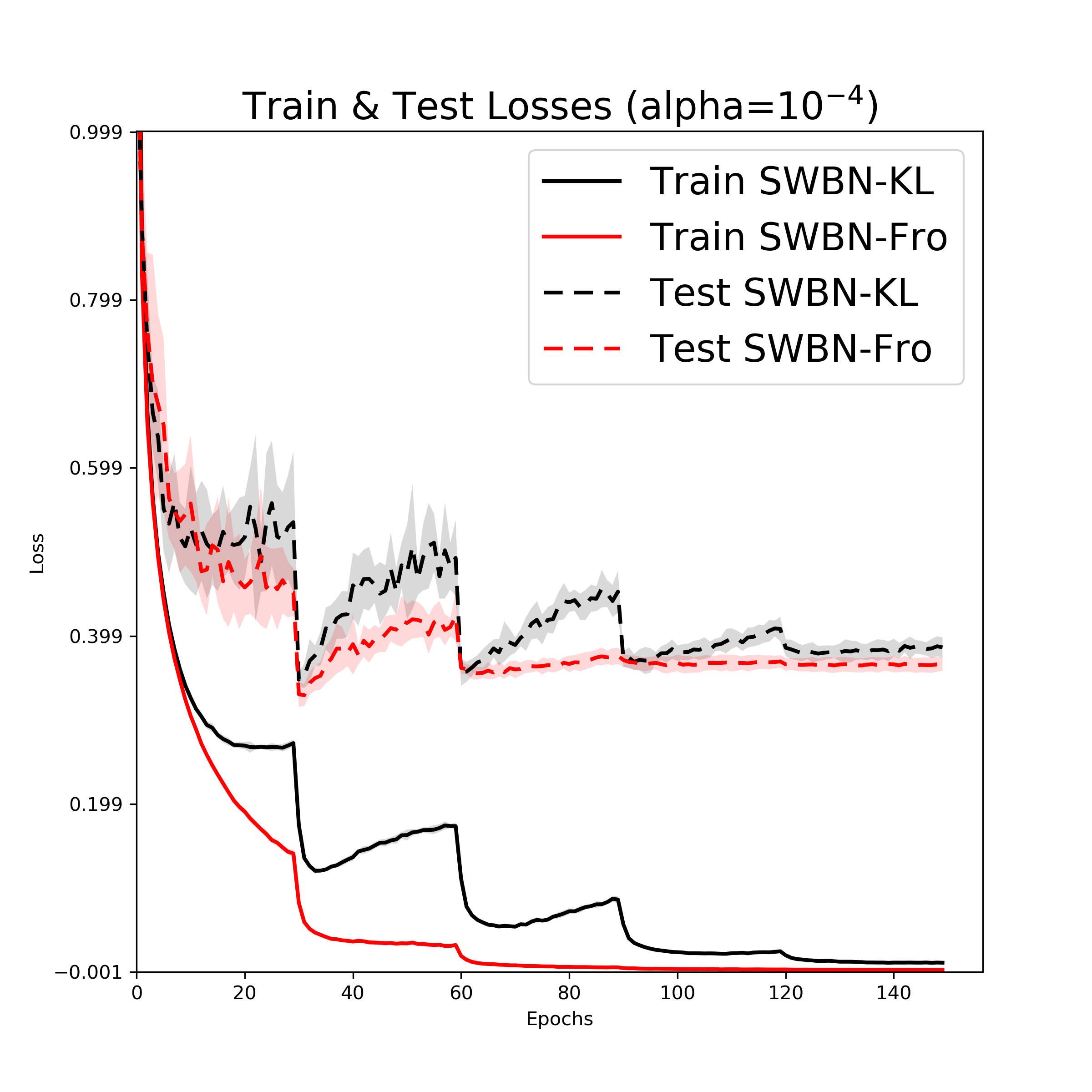
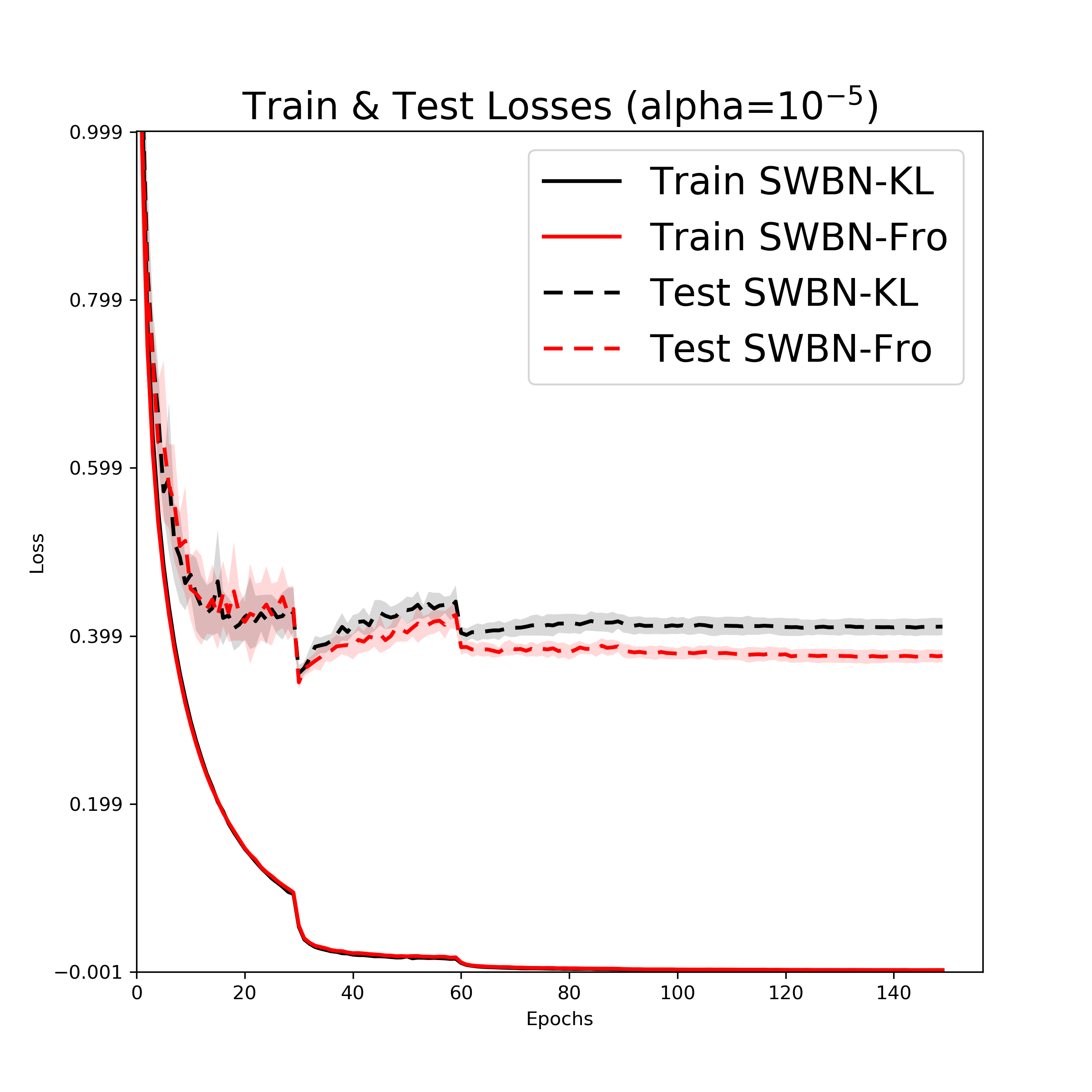
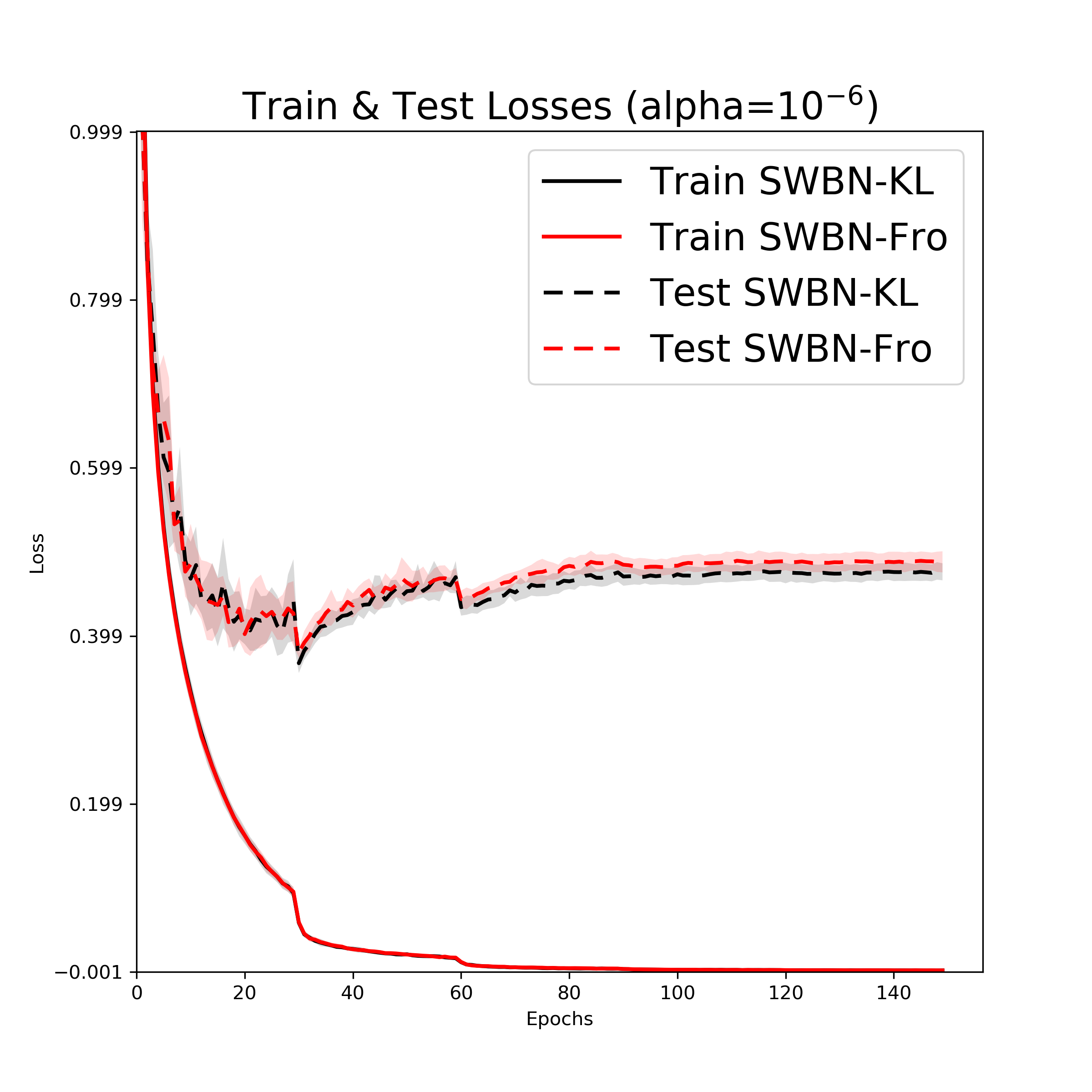
Figure 2: Effect of whitening step sizes on training and test loss. The plots show the mean curves of $10$ runs with $\pm 1$ standard deviation. Best viewed in color.

4.1.2 Effect of Batch Size

We also show the effect of different batch sizes on the performance of SWBN. We also include the results of IterNorm for comparison. We follow the same configuration, except each experiment is run for $150$ epochs, and the learning rate is divided by $10$ at every $30$ epochs. The loss curves with $1$ standard deviation error bars for batch sizes $32$, $128$ and $512$ are shown in Figure 3. As seen, the lowest test losses for different batch sizes are achieved by SWBN-Fro. The models with SWBN layers outperform those with BN and IterNorm layers in terms of test loss.

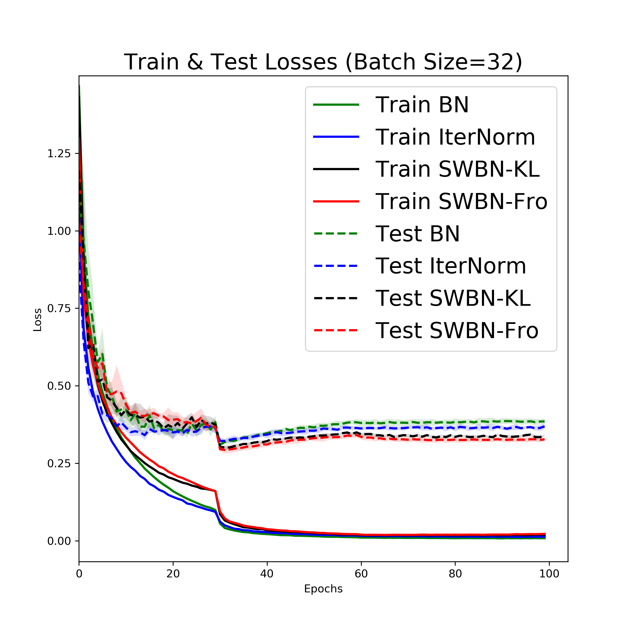
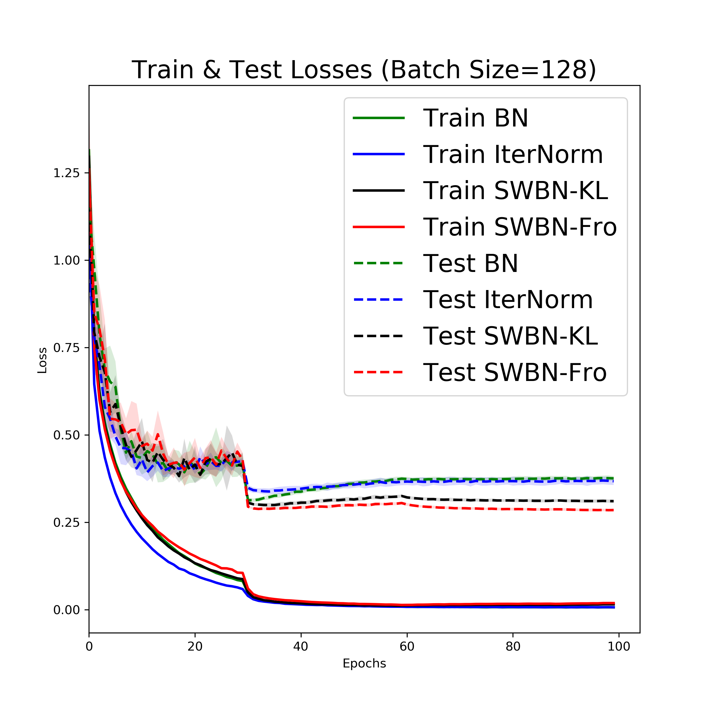
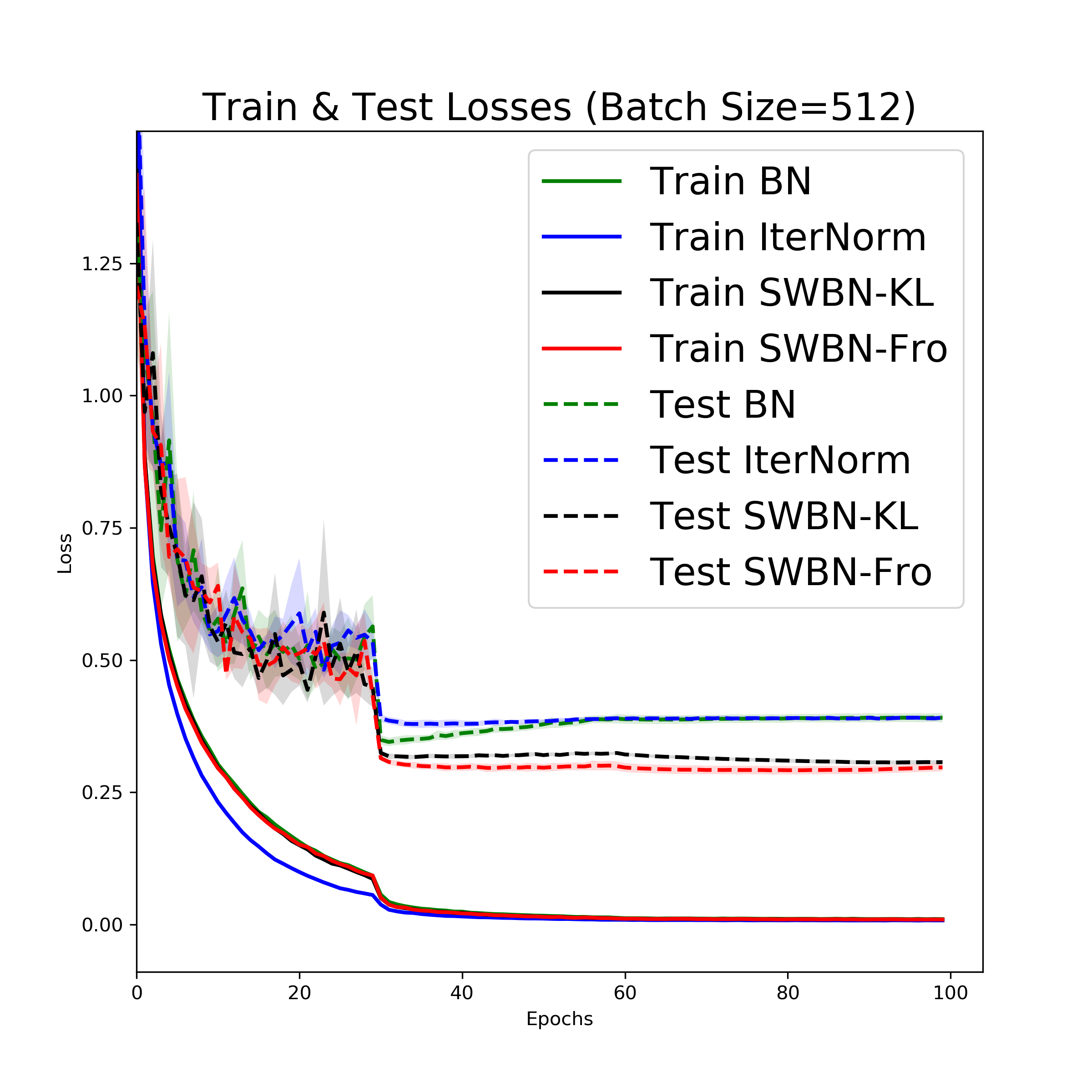
Figure 3: Effect of different batch sizes. The plots show the mean curves of 5 runs with $\pm 1$ standard deviation. Best viewed in color.

4.1.3 Whitening Effect of SWBN

To demonstrate the whitening effect of the SWBN algorithm, we feed in random $5000$ CIFAR-$10$ images to a trained VGG model, and extract its output of the last normalization layer, i.e. the features before being scaled and shifted by parameters $\vec{\gamma}$ and $\vec{\beta}$, respectively. Figure 4 shows the heatmap plots of the correlation matrices generated from the hidden features before training (i.e., epoch 0), and after $150$ epochs. For better visualization, we only show the correlation heatmaps for randomly selected $128$ features. In these plots, darker pixels represent smaller values in the correlation matrix. The plots in the first column show that BN layers can not whiten the feature maps as batch normalized features remain highly correlated throughout training. The second and third columns of the plots show that the correlation matrices of the features after the SWBN layers are close to the identity matrix, indicating that the features are highly whitened.

Epoch $0$

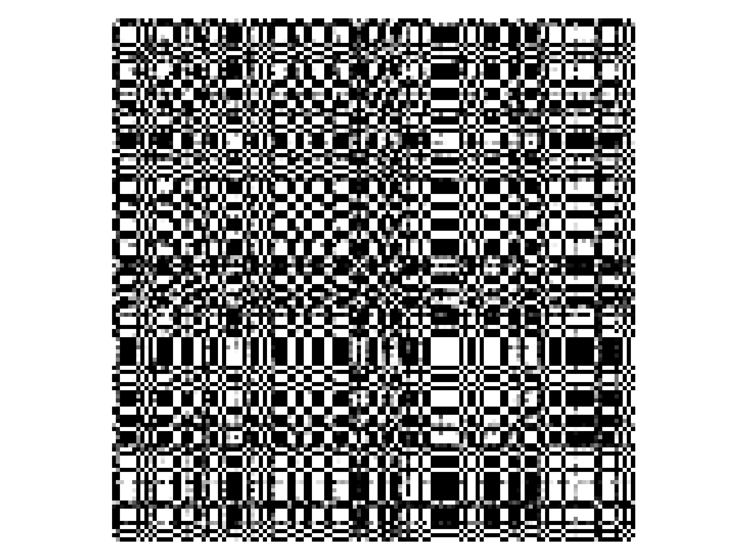
Epoch $150$

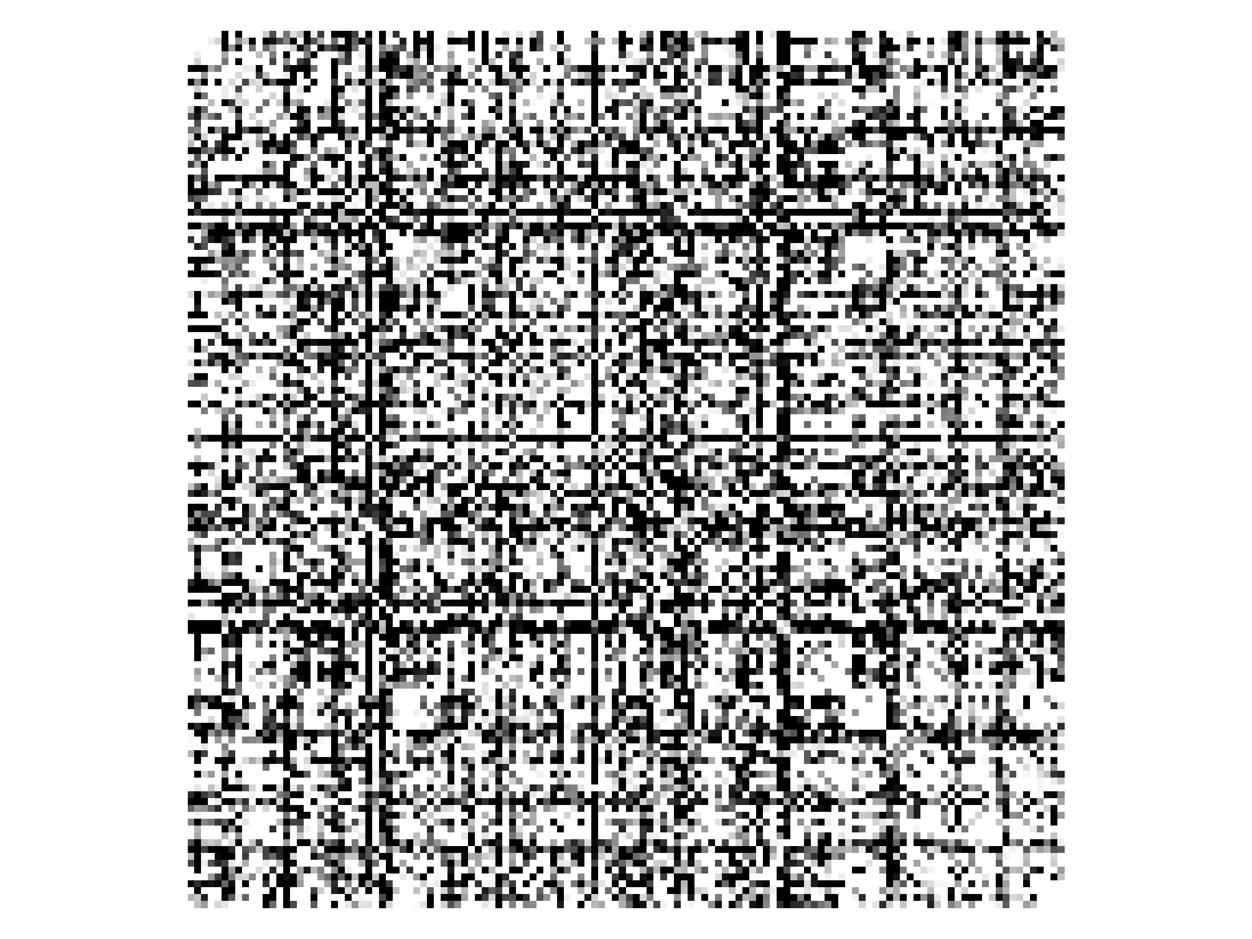
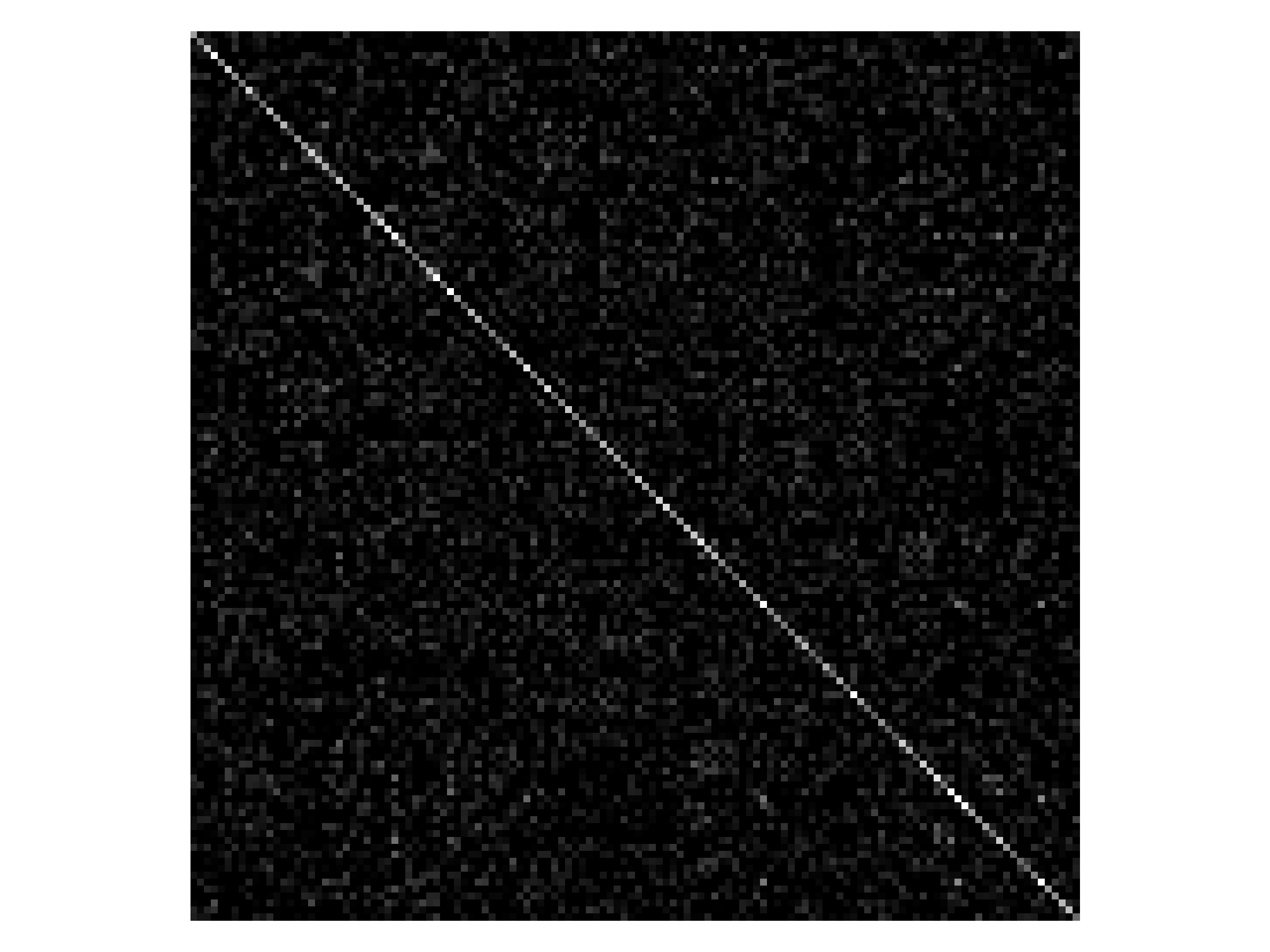
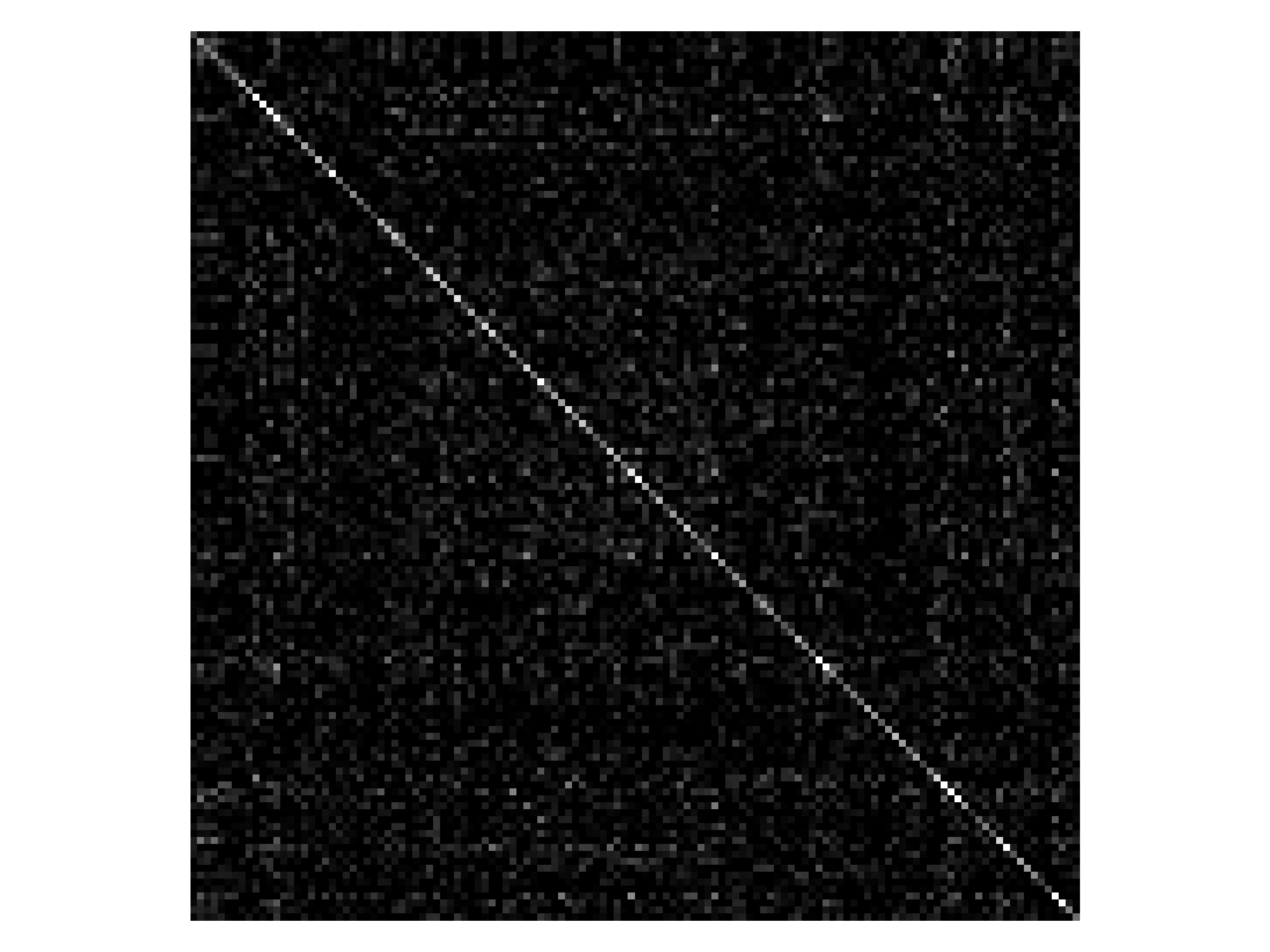
(a)           BN                   SWBN-KL                SWBN-Fro

Figure 4: Comparison of heatmaps of correlation matrices. Columns, from left to right, represent heatmaps for the models with BN, SWBN-KL, and SWBN-Fro layers, respectively. Rows, from top to bottom, represent heatmaps of the corresponding models before and after training, respectively.

4.1.4 Wall-clock Time Comparison

To demonstrate the efficiency of SWBN, we perform a series of experiments to measure the training time of SWBN and IterNorm. We follow the same procedures as described in [15] to measure wall-clock time. We use TITAN Xp with Pytorch v$1.3$ and CUDA $10.1$ for the experiments. We define the input tensor $X\in\mathbf{R}^{h\times w\times d\times m}$ and the $3\times 3$ convolutional tensor $W\in\mathbf{R}^{3\times 3\times d\times d}$, where $h=w=32$, $d$ and $m=64$ are height, width, number of channels and batch size, respectively. Pytorch implementations of SWBN and IterNorm are used to run these experiments. For each dimension $d\in\{256,1024,2048\}$, wall-clock time of one forward pass plus backward pass for a single layer is averaged over $100$ runs. Experimental results are summarized in Table 1.

	d=256	d=1024	d=2048
BatchNorm	1.7ms	5.01ms	11.44ms
SWBN-KL	13.5ms	72.5ms	256.4ms
SWBN-Fro	13.2ms	72.3ms	260.12ms
IterNorm	15.5ms	111.8ms	475.34ms

Table 1: Single layer wall-clock time (in ms), averaged over $100$ runs, for BatchNorm, IterNorm and SWBN.

CIFAR-10 (1 GPU)	SWBN-KL	SWBN-Fro	IterNorm
ResNetV2-164	123s	125s	187s
WRN-40-10	226s	230s	299s
ImageNet (8 GPUs)	SWBN-KL	SWBN-Fro	IterNorm
ResNetV2-50	27min	31min	97min
ResNetV2-101	38min	43min	184min

Table 2: Training time per epoch of IterNorm and SWBN layers on CIFAR-10 and ImageNet datasets, averaged over $3$ runs.

To show the efficiency of SWBN with popular DNN models, we select the wide architecture Wide ResNet(WRN) [36] and the deep architecture ResNetV2 [12]. All BN layers in these models are replaced with SWBN and IterNorm, and the models are trained on CIFAR-$10$ dataset with images of size $32\times 32\times 3$. Further, we do the same experiments with ResNetV2 on the ImageNet dataset with images of size $224\times 224\times 3$. The batch size is fixed to $128$ for CIFAR-$10$ and $256$ for ImageNet. On ImageNet, we use $8$ Tesla V$100$ GPUs for acceleration. Table 2 summarizes training time of one epoch for models with different whitening layers. As seen, SWBN models are significantly faster than their IterNorm counterparts, especially for very deep CNNs with a large input size.

4.2 Image Classification

In this section, we evaluate the performance of SWBN on image classification benchmarks CIFAR-$10$, CIFAR-$100$ and ILSVRC-$2012$ (ImageNet). The performance of SWBN is compared with that of the state-of-the-art whitening methods, such as DBN [14] and IterNorm [15].

4.2.1 CIFAR-$10$ and CIFAR-$100$

In this section, we provide SWBN’s performance on CIFAR-$10$ and CIFAR-$100$ datasets using deep and wide CNNs. We select a deep model architecture, ResNetV2 [12], and a wide model architecture, Wide ResNet (WRN) [36]. We use the same architecture as reported in [36] and [12], and replace all BN layers with SWBN or IterNorm layers. CIFAR-$100$ is a variant dataset of CIFAR-$10$, which has $60$K color images of size $32\times 32$: $50$K in the training set and $10$K in the test set. The task is to classify images into $100$ categories instead of $10$, making it more challenging than CIFAR-$10$ because there are fewer data samples for each category. Every experiment was repeated $10$ times with different random seeds. The mean test accuracies are reported in Tables 4 and 4. We use the same training configuration, hyper-parameters and data augmentation setups as described in the original papers. The whitening step size $\alpha$ is set to $10^{-5}$ for all the experiments. Because no results on CIFAR-$100$ dataset are reported in [15], we used the released code from [15] to run these experiments. We don’t conduct additional experiments for DBN because IterNorm is faster and has better performance [15].

As shown in Table 4, for CIFAR-$10$ dataset models with SWBN layers generally outperform the ones with BN layers, and have similar performance as those with IterNorm layers. However, as shown in Table 4, for CIFAR-$100$ dataset, SWBN layers improve the generalization performance of these models. Surprisingly, IterNorm layers reduce the generalization performance of deep CNN models like ResNetV$2$ comparing with BN layers.

Models	BN Baseline	DBN	IterNorm	SWBN-KL	SWBN-Fro
ResNetV2-56	92.92	N/A	$93.11^{*}$	93.4	93.23
ResNetV2-164	94.54 [12]	N/A	$94.45^{*}$	94.68	94.59
WRN-28-10	96.11 [36]	96.21 [14]	$96.19^{*}$	96.23	96.18
WRN-40-10	96.2 [36]	96.26 [14]	$96.23^{*}$	96.39	96.35

Table 3: CIFAR-$10$ Results. All numbers for SWBN models are averaged test accuracies (%) of $10$ runs. Best average accuracies are highlighted in bold face, and N/A indicates that the accuracy is not reported in the referenced paper. ^∗ indicates results produced by the released code of [15].

Models	BN Baseline	IterNorm	SWBN-KL	SWBN-Fro
ResNetV2-56	73.01	$72.1^{*}$	73.12	72.9
ResNetV2-164	75.56	$74.12^{*}$	76.13	76.02
WRN-28-10	81.15 [36]	$79.83^{*}$	81.41	81.31
WRN-40-10	81.7 [36]	$80.56^{*}$	81.7	81.78

Table 4: CIFAR-$100$ Results. All numbers for SWBN models are average test accuracies (%) of $10$ runs. Best average accuracies are highlighted in bold face. ^∗ indicates results produced by the released code of [15]. The BN baseline accuracies reported for WRN in [36] are the best single run results.

4.2.2 ILSVRC-$2012$ (ImageNet)

In this section, we compare SWBN with IterNorm on ILSVRC-$2012$, a.k.a. ImageNet dataset. The dataset has $1.28$ million images for training and $50,000$ images for testing. The task is to classify an image into $1000$ classes.

In [15], to speed up the training of ResNet [11] with IterNorm on this dataset, the authors only replaced the first BN layer with an IterNorm layer and added one IterNorm layer before the last linear layer, a total of two IterNorm layers used in their models. To make a fair comparison, we use the same setting, by replacing $2$ BN layers with SWBN layers at the exact locations in the model. The results are shown in the first row of Table 5.

To further test the scalability and performance improvement of SWBN for larger state-of-the-art models, we train two ResNeXt models [33] with SWBN layers. We employ the same configuration as defined in [33], and choose ResNeXt-$50$, $32$x$4$d and ResNeXt-$101$, $32$x$4$d, which have $\sim 25$M and $\sim 44$M parameters, respectively. Experimental configurations can be found in Appendix D.

Both top-$1$ and top-$5$ test accuracies are reported in Table 5. The test accuracies were evaluated on the single-cropped $224\times 224$ test images. As seen, the ResNeXt models that use SWBN layers outperform the ones with BN layers, both in top-1 and top-5 accuracies. This validates the scalability of the proposed SWBN layer for large networks and datasets. We were not able to perform identical experiments for IterNorm on ResNeXt due to high computational cost of IterNorm, as discussed in Section 3.6 and indicated in Table 1 and 2.

Model	BN		IterNorm		SWBN-KL		SWBN-Fro
	top-1	top-5	top-1	top-5	top-1	top-5	top-1	top-5
ResNet-50	75.3 [10]	92.2 [10]	77.09 [15]	93.53 [15]	77.03	93.61	76.95	93.23
ResNeXt-50	77.8	N/A	N/A	N/A	78.1	93.71	78.2	93.68
ResNeXt-101	78.8	94.4	N/A	N/A	79.39	94.51	79.27	94.48

Table 5: Single run results of ILSVRC-$2012$. N/A indicates the accuracy is not reported in the referenced paper or not available for high computational cost.

4.3 Few-shot Classification

Few-shot classification aims to recognize unlabeled samples of newly observed classes given only one or a few labeled samples. Unknown data distributions of unseen classes and the scarce amount of labeled data make few-shot classification particularly difficult. In terminology of the few-shot classification, if the few-shot training (a.k.a support) dataset contains K labeled samples for each of C categories, the target few-shot task is called a C-way K-shot task. Metric learning, which stands for approaches designed to learn transferable data representations, is commonly used to tackle this task. Siamese networks [20], matching networks [30], and prototypical networks [28] are examples of metric learning models. Recently proposed cross attention networks [13] shows the-state-of-the-art performance on benchmark datasets. Most of these approaches require training backbone networks for extracting representations from input data. We choose matching networks, prototypical networks, and cross attention networks with small backbone networks to compare the performance of BN, SWBN, and IterNorm layers. Experimental details are included in Appendix D. Table 6 shows results on two few-shot classification benchmark datasets, namely mini-Imagenet and CIFAR-FS. We choose Resnet12 and Resnet20 as the backbone networks for mini-Imagenet and CIFAR-FS, respectively. As shown in Table 6, all the whitening layers outperform the BN layer, and SWBN-Fro is generally better than IterNorm while having lower memory consumption and better computational efficiency.

Dataset	Approach	Backbone	BN		SWBN-KL		SWBN-Fro		IterNorm
			5W1S	5W5S	5W1S	5W5S	5W1S	5W5S	5W1S	5W5S
mini- Imagenet	MN [30]	Resnet12	57.37	68.22	57.79	68.88	57.55	68.47	57.49	68.64
	PN [28]		55.29	73.63	55.44	73.74	56.55	74.5	55.66	73.26
	CAN [13]		62.58	78.64	64.37	79.19	64.97	79.22	64.12	79.64
CIFAR-FS	MN [30]	Resnet20	61.28	72.8	62.32	73.98	62.73	74.26	62.35	74.21
	PN [28]		55.73	73.47	56.76	74.51	57.38	75.02	56.61	74.48
	CAN [13]		65.28	79.39	65.71	79.84	66.08	80.45	65.95	80.76

Table 6: Results of mini-Imagenet and CIFAR-FS datasets. Best test accuracies are highlighted in bold face. The abbreviations in the Approach column stand for: matching network (MN), prototypical network (PN), and cross attention network (CAN). $c$W$k$S stands for $c$-way $k$-shot.

5 Conclusions

In this paper, we propose the Stochastic Whitening Batch Normalization (SWBN) technique with two whitening criteria $C_{KL}$ and $C_{Fro}$. SWBN is a new extension to Batch Normalization (BN), which further whitens data in an online fashion. The proposed data whitening algorithm outperforms the newly proposed IterNorm in terms of computational efficiency. The SWBN layers accelerate training convergence of deep neural networks and enable them to have better generalization performance by incrementally whitening and rescaling activations. Ablation experiments demonstrate that SWBN is capable of efficiently whitening data in a stochastic way. The wall-clock time records show that SWBN is more efficient than IterNorm. We also show the performance improvement by replacing BN layers inside the state-of-the-art CNN models with SWBN layers on CIFAR-$10$/$100$ and the ImageNet dataset, as well as few-shot classification benchmark datasets mini-Imagenet and CIFAR-FS.

References

- [1] J. Ba, R. Kiros, and G. E. Hinton. Layer normalization. ArXiv, abs/1607.06450, 2016.
- [2] A. J. Bell and T. J. Sejnowski. The “independent components” of natural scenes are edge filters. Vision research, 37(23):3327–3338, 1997.
- [3] L. Bertinetto, J. F. Henriques, P. H. Torr, and A. Vedaldi. Meta-learning with differentiable closed-form solvers. arXiv preprint arXiv:1805.08136, 2018.
- [4] J.-F. Cardoso and B. H. Laheld. Equivariant adaptive source separation. IEEE Transactions on signal processing, 44(12):3017–3030, 1996.
- [5] V. Chiley, I. Sharapov, A. Kosson, U. Koster, R. Reece, S. Samaniego de la Fuente, V. Subbiah, and M. James. Online normalization for training neural networks. Advances in Neural Information Processing Systems, 32:8433–8443, 2019.
- [6] M. Cogswell, F. Ahmed, R. B. Girshick, L. Zitnick, and D. Batra. Reducing overfitting in deep networks by decorrelating representations. In 4th International Conference on Learning Representations, ICLR 2016, San Juan, Puerto Rico, May 2-4, 2016, Conference Track Proceedings, 2016.
- [7] J. Deng, W. Dong, R. Socher, L.-J. Li, K. Li, and L. Fei-Fei. ImageNet: A Large-Scale Hierarchical Image Database. In IEEE/CVF Conference on Computer Vision and Pattern Recognition, 2009.
- [8] G. Desjardins, K. Simonyan, R. Pascanu, and k. kavukcuoglu. Natural neural networks. In C. Cortes, N. D. Lawrence, D. D. Lee, M. Sugiyama, and R. Garnett, editors, Advances in Neural Information Processing Systems 28, pages 2071–2079. Curran Associates, Inc., 2015.
- [9] Y. C. Eldar and A. V. Oppenheim. Mmse whitening and subspace whitening. IEEE Transactions on Information Theory, 49(7):1846–1851, 2003.
- [10] K. He, R. S. Zhang, Xiangyu, and J. Sun. Deep Residual Networks.
- [11] K. He, X. Zhang, S. Ren, and J. Sun. Deep residual learning for image recognition. In Proceedings of the IEEE conference on computer vision and pattern recognition, pages 770–778, 2016.
- [12] K. He, X. Zhang, S. Ren, and J. Sun. Identity mappings in deep residual networks. In European conference on computer vision, pages 630–645. Springer, 2016.
- [13] R. Hou, H. Chang, M. Bingpeng, S. Shan, and X. Chen. Cross attention network for few-shot classification. In Advances in Neural Information Processing Systems, pages 4003–4014, 2019.
- [14] L. Huang, D. Yang, B. Lang, and J. Deng. Decorrelated batch normalization. In Proceedings of the IEEE Conference on Computer Vision and Pattern Recognition, pages 791–800, 2018.
- [15] L. Huang, Y. Zhou, F. Zhu, Y. Liu, and L. Shao. Iterative normalization: Beyond standardization towards efficient whitening. In Proceedings of the IEEE Conference on Computer Vision and Pattern Recognition, pages 4874–4883, 2019.
- [16] S. Ioffe. Batch renormalization: Towards reducing minibatch dependence in batch-normalized models. In I. Guyon, U. V. Luxburg, S. Bengio, H. Wallach, R. Fergus, S. Vishwanathan, and R. Garnett, editors, Advances in Neural Information Processing Systems 30, pages 1945–1953. Curran Associates, Inc., 2017.
- [17] S. Ioffe and C. Szegedy. Batch normalization: Accelerating deep network training by reducing internal covariate shift. pages 448–456, 2015.
- [18] I. Jolliffe. Principal Component Analysis. Springer Berlin Heidelberg, Berlin, Heidelberg, 2011.
- [19] A. Kessy, A. Lewin, and K. Strimmer. Optimal whitening and decorrelation. The American Statistician, 72(4):309–314, 2018.
- [20] G. Koch. Siamese neural networks for one-shot image recognition. 2015.
- [21] A. Krizhevsky, V. Nair, and G. Hinton. Cifar-10 (canadian institute for advanced research).
- [22] Y. LeCun, L. Bottou, G. B. Orr, and K.-R. Müller. Efficient backprop. In Neural Networks: Tricks of the Trade, This Book is an Outgrowth of a 1996 NIPS Workshop, pages 9–50, London, UK, UK, 1998. Springer-Verlag.
- [23] Q. Liao, K. Kawaguchi, and T. A. Poggio. Streaming normalization: Towards simpler and more biologically-plausible normalizations for online and recurrent learning. ArXiv, abs/1610.06160, 2016.
- [24] P. Luo. Learning deep architectures via generalized whitened neural networks. In D. Precup and Y. W. Teh, editors, Proceedings of the 34th International Conference on Machine Learning, volume 70 of Proceedings of Machine Learning Research, pages 2238–2246, International Convention Centre, Sydney, Australia, 06–11 Aug 2017. PMLR.
- [25] T. Raiko, H. Valpola, and Y. Lecun. Deep learning made easier by linear transformations in perceptrons. In N. D. Lawrence and M. Girolami, editors, Proceedings of the Fifteenth International Conference on Artificial Intelligence and Statistics, volume 22 of Proceedings of Machine Learning Research, pages 924–932, La Palma, Canary Islands, 21–23 Apr 2012. PMLR.
- [26] T. Salimans and D. P. Kingma. Weight normalization: A simple reparameterization to accelerate training of deep neural networks. In D. D. Lee, M. Sugiyama, U. V. Luxburg, I. Guyon, and R. Garnett, editors, Advances in Neural Information Processing Systems 29, pages 901–909. Curran Associates, Inc., 2016.
- [27] S. Shen, Z. Yao, A. Gholami, M. Mahoney, and K. Keutzer. Powernorm: Rethinking batch normalization in transformers. In International Conference on Machine Learning, pages 8741–8751. PMLR, 2020.
- [28] J. Snell, K. Swersky, and R. Zemel. Prototypical networks for few-shot learning. In Advances in neural information processing systems, pages 4077–4087, 2017.
- [29] N. Srivastava, G. Hinton, A. Krizhevsky, I. Sutskever, and R. Salakhutdinov. Dropout: a simple way to prevent neural networks from overfitting. The Journal of Machine Learning Research, 15(1):1929–1958, 2014.
- [30] O. Vinyals, C. Blundell, T. Lillicrap, D. Wierstra, et al. Matching networks for one shot learning. In Advances in neural information processing systems, pages 3630–3638, 2016.
- [31] W. Wang, Z. Dang, Y. Hu, P. Fua, and M. Salzmann. Backpropagation-friendly eigendecomposition. In Advances in Neural Information Processing Systems, pages 3162–3170, 2019.
- [32] Y. Wu and K. He. Group normalization. In Proceedings of the European Conference on Computer Vision (ECCV), pages 3–19, 2018.
- [33] S. Xie, R. Girshick, P. Dollár, Z. Tu, and K. He. Aggregated residual transformations for deep neural networks. In Proceedings of the IEEE conference on computer vision and pattern recognition, pages 1492–1500, 2017.
- [34] W. Xiong, B. Du, L. Zhang, R. Hu, and D. Tao. Regularizing deep convolutional neural networks with a structured decorrelation constraint. 2016 IEEE 16th International Conference on Data Mining (ICDM), pages 519–528, 2016.
- [35] Y. Yoshida and T. Miyato. Spectral norm regularization for improving the generalizability of deep learning. arXiv preprint arXiv:1705.10941, 2017.
- [36] S. Zagoruyko and N. Komodakis. Wide residual networks. arXiv preprint arXiv:1605.07146, 2016.