Estimating Reeb Chords using Microlocal Sheaf Theory

Abstract.

We show that for a closed Legendrian submanifold in a 1-jet bundle, if there is a sheaf with compact support, perfect stalk and singular support on that Legendrian, then (1) the number of Reeb chords has a lower bound by half of the sum of Betti numbers of the Legendrian; (2) the number of Reeb chords between the original Legendrian and its Hamiltonian pushoff has a lower bound in terms of Betti numbers when the oscillation norm of the Hamiltonian is small comparing with the length of Reeb chords. In the proof we develop a duality exact triangle and use the persistence structure (which comes from the action filtration) of microlocal sheaves.

1. Introduction

1.1. Motivation and Background

A contact manifold $(Y,\xi)$ is a $(2n+1)$-manifold $Y$ together with a maximal nonintegrable hyperplane distribution $\xi$. Assume that there exists a 1-form $\alpha\in\Omega^{1}(Y)$ called a contact form such that $\xi=\ker\alpha$ (this is equivalent to saying that $\xi$ is coorientable). Given a contact form $\alpha$, we define the Reeb vector field $R_{\alpha}$ to be the vector field satisfying

$$\iota(R_{\alpha})\alpha=1,\,\,\,\iota(R_{\alpha})(d\alpha)=0.$$

In a contact manifold $(Y,\ker\alpha)$, we consider Legendrian submanifolds $\Lambda\subset Y$ that are $n$-manifolds such that $T\Lambda\subset\xi|_{\Lambda}$. Reeb chords on $\Lambda$ are Reeb trajectories that both start and end on $\Lambda$.

Estimating the number of Reeb chords has been a basic question on Legendrian submanifolds since Arnold’s time [Arnold]. When the contact manifold is $(Y,\xi)=(P\times\mathbb{R}_{t},\ker(dt-\theta_{P}))$ where $(Y,d\theta_{P})$ is an exact symplectic manifold, one can pick the contact form $\alpha=dt-\theta_{P}$, and then the Reeb vector field is $\partial/\partial t$. For $\Lambda$ a closed Legendrian, consider the Lagrangian projection

$$\pi_{\text{Lag}}:\Lambda\hookrightarrow P\times\mathbb{R}\rightarrow P.$$

The Reeb chords between Legendrian submanifolds correspond bijectively to intersection points of their Lagrangian projections.

For the number of self Reeb chords, when $n$ is even, there is a topological lower bound coming from $[\pi_{\text{Lag}}(\Lambda)]\cdot[\pi_{\text{Lag}}(\Lambda)]=\chi(\Lambda)/2$. Some flexibility results tell us that this is sometimes the best bound one can expect [Fewdoublepoints]. However, under some extra assumptions, there are rigid behaviours beyond this purely algebraic topological bound.

Using pseudo-holomorphic curves, a number of celebrated theorems on the number of self Reeb chords have been found [Mohnkechord, Cieliechord, Rittertqft]. In particular, for Legendrians $\Lambda\subset P\times\mathbb{R}$, using Legendrian contact homology, works by Ekholm-Etnyre-Sullivan, Ekholm-Etnyre-Sabloff and Dimitroglou Rizell-Golovko [EESorientation, EESduality, RizGolestimating] showed that, under some assumptions, the number of self Reeb chords is bounded from below by half of the sum of Betti numbers.

Other than estimating self Reeb chords, estimating the number of Reeb chords between $\Lambda$ and some Hamiltonian pushoff $\varphi_{H}^{1}(\Lambda)$ has also been an important question. When the contact Hamiltonian comes from a symplectic Hamiltonian on $P$, this question reduces to the Arnold conjecture for (immersed) Lagrangian submanifolds $\pi_{\text{Lag}}(\Lambda)$ [Arnold].

Many Legendrians can be displaced from themselves so that there are no Reeb chords between $\Lambda$ and $\varphi_{H}^{1}(\Lambda)$. However, when the norm of the Hamiltonian is sufficiently small, one can get estimates on the number of Reeb chords between $\Lambda$ and $\varphi_{H}^{1}(\Lambda)$ using pseudo-holomorphic curves [Akaho, Chekanov, LiuCuplength, RizSenergy]. In particular a recent result by Dimitroglou Rizell-Sullivan [RizSpersist], using the persistence of Legendrian contact homology, showed that for Legendrians $\Lambda\subset P\times\mathbb{R}$, under certain assumptions, there is a lower bound of the number of Reeb chords in terms of Betti numbers, when the oscillation norm of the Hamiltonian is small comparing to the length of Reeb chords.

On the other hand, in recent years microlocal sheaf theory has also shown to be a powerful tool in symplectic and contact geometry [NadZas, Nad, Tamarkin1, Shendeconormal, STZ, STWZ, Gui, GuiGEthm, Guithree, Chiu, Arborealloose, CasalsZas]. In symplectic geometry, microlocal sheaf theory has already been used to show estimations on number of intersection points of Lagrangians (in particular, to solve non-displaceability problems) [Tamarkin1, GKS, GS, AsanoIkeimmersion].

In contact geometry, conjecturally microlocal sheaves should be equivalent to certain representations of the Chekanov-Eliashberg dg algebra defined by pseudo-holomorphic curves, and for $\mathbb{R}^{3}_{\text{std}}$ it is known that a category of augmentations of the Chekanov-Eliashberg dg algebra is indeed a microlocal sheaf category consisting of microlocal rank 1 (i.e. simple) objects [AugSheaf] (in higher dimensions, also some results can be obtained [CasalsMurphydga, AugSheafknot, AugSheafsurface]). Therefore one may expect that we can use sheaf theory to study the number of Reeb chords.

However, even though conjecturally augmentations are sheaves, it doesn’t seem clear how the homomorphisms of sheaves should correspond to Reeb chords geometrically. The main purpose of this paper is to set up the correspondence and estimate the number of Reeb chords using microlocal sheaf theory.

1.2. Results and Methods

We will show the following theorems on Reeb chord estimations, using microlocal sheaf theory. In order to apply microlocal sheaf theory, we consider only contact manifolds $J^{1}(M)=T^{*}M\times\mathbb{R}$ where $\dim M=n$, which are contactomorphic to

$$T^{*,\infty}_{\tau>0}(M\times\mathbb{R})=\{(x,t,\xi,\tau)||\xi|^{2}+|\tau|^{2}=1,\tau>0\}.$$

The contact form we choose will be $\alpha=dt-(\xi/\tau)dx$, and thus the Reeb vector field is $R_{\alpha}=\partial/\partial t$. Recall that the support of a complex of sheaves in $M\times\mathbb{R}$ is

$$\mathrm{supp}(\mathscr{F})=\overline{\bigcup_{j\in\mathbb{Z}}\{x\in M\times\mathbb{R}|(H^{j}\mathscr{F})_{x}\neq 0\}}.$$

Remark 1.1.

Throughout the paper, $Sh^{b}_{\Lambda}(M\times\mathbb{R})$ will represent the dg category of sheaves over $\Bbbk$ with perfect cohomologies, localized along acyclic objects.

For self Reeb chords of a Legendrian $\Lambda\subset T^{*,\infty}_{\tau>0}(M\times\mathbb{R})$, we have the following results analogous to Ekholm-Etnyre-Sullivan [EESorientation], Ekholm-Etnyre-Sabloff [EESduality] and Dimitroglou Rizell-Golovko [RizGolestimating], where they showed the same inequality under the existence of a finite dimensional representation of the Chekanov-Eliashberg dg algebra, or Sabloff-Traynor [Genfamily] where they used generating families.

A Legendrian submanifold $\Lambda\subset T^{*,\infty}_{\tau>0}(M\times\mathbb{R})$ is chord generic, if the Lagrangian projection $\pi_{\text{Lag}}(\Lambda)$ is immersed with only transverse double points. Let $\mathcal{Q}(\Lambda)$ be the set of Reeb chords on $\Lambda$. Assume that the Maslov class $\mu(\Lambda)=0$. Then there is a grading on Reeb chords of $\Lambda$ (where the degree is given by the Conley-Zehnder index; see Section 2.3). Let $\mathcal{Q}_{i}(\Lambda)$ be the set of degree $i$ Reeb chords on $\Lambda$.

Theorem 1.1.

Let $M$ be orientable, $\Lambda\subset T^{*,\infty}_{\tau>0}(M\times\mathbb{R})$ be a closed chord generic Legendrian submanifold and $\Bbbk$ be a field (and $\Lambda$ is spin when $\mathrm{char}\Bbbk\neq 2$). If there exists a $\Bbbk$-coefficient pure sheaf $\mathscr{F}\in Sh^{b}_{\Lambda}(M\times\mathbb{R})$ with microlocal rank $r$ such that $\mathrm{supp}(\mathscr{F})$ is compact, then

$$|\mathcal{Q}_{i}(\Lambda)|+|\mathcal{Q}_{n-i}(\Lambda)|\geq b_{i}(\Lambda;\Bbbk).$$

In particular, the number of Reeb chords

$$|\mathcal{Q}(\Lambda)|\geq\frac{1}{2}\sum_{i=0}^{n}b_{i}(\Lambda;\Bbbk).$$

Here $b_{i}(\Lambda;\Bbbk)=\dim_{\Bbbk}H^{i}(\Lambda;\Bbbk)$.

Theorem 1.2.

Let $M$ be orientable, $\Lambda\subset T^{*,\infty}_{\tau>0}(M\times\mathbb{R})$ be a closed chord generic Legendrian submanifold and $\Bbbk$ be a field (and $\Lambda$ is spin when $\mathrm{char}\Bbbk\neq 2$). If there exists a $\Bbbk$-coefficient sheaf $\mathscr{F}\in Sh^{b}_{\Lambda}(M\times\mathbb{R})$ with perfect stalk such that $\mathrm{supp}(\mathscr{F})$ is compact, then

$$|\mathcal{Q}(\Lambda)|\geq\frac{1}{2}\sum_{i=0}^{n}b_{i}(\Lambda;\Bbbk).$$

Here $b_{i}(\Lambda;\Bbbk)=\dim_{\Bbbk}H^{i}(\Lambda;\Bbbk)$.

Remark 1.2.

The condition that $\mathrm{supp}(\mathscr{F})$ is compact may be thought of as an analogue of the linear at infinity condition on generating families [Genfamily]. If we drop this condition, then there will be counterexamples. Consider the positive conormal $\nu^{*,\infty}_{M,\tau>0}(M\times\mathbb{R})\subset T^{*,\infty}_{\tau>0}(M\times\mathbb{R})$ (which is just the zero section $M\subset J^{1}(M)$). There is an obvious sheaf $\Bbbk_{M\times[0,+\infty)}$ with the prescribed singular support. However that Legendrian has no Reeb chords.

Remark 1.3.

When there is a sheaf $\mathscr{F}\in Sh^{b}_{\Lambda}(M\times\mathbb{R})$ with perfect stalk, then one can show that [Gui] necessarily the Maslov class $\mu(\Lambda)=0$. However this condition is not necessary to get estimates on number of Reeb chords. In general, one can consider the triangulated orbit category $Sh^{b}_{\Lambda}(M\times\mathbb{R})_{/[1]}$ consisting of sheaves of $1$-cyclic complexes (see [Orbitcat] and [Gui, Section 3]). When there is a sheaf $\mathscr{F}\in Sh^{b}_{\Lambda}(M\times\mathbb{R})_{/[1]}$, then we still expect that

$$|\mathcal{Q}(\Lambda)|\geq\frac{1}{2}\sum_{i=0}^{n}b_{i}(\Lambda;\Bbbk),$$

but we do not work out the details here.

Remark 1.4.

In [EESorientation, EESduality, RizGolestimating] they imposed the condition that the Legendrian $\Lambda$ is horizontally displaceable, meaning that there exists a Hamiltonian isotopy $\varphi_{H}^{s}\,(s\in I)$ such that there are no Reeb chords between $\Lambda$ and $\varphi_{H}^{1}(\Lambda)$. In Section 6.4 we show that if $\Lambda$ is horizontally displaceable, then any $\mathscr{F}\in Sh^{b}_{\Lambda}(M\times\mathbb{R})$ necessarily has compact support.

However, there are Legendrians that are not horizontally displaceable but admit sheaves with compact support. For example let

$$T_{c}:M\times\mathbb{R}\rightarrow M\times\mathbb{R},\,\,(x,t)\mapsto(x,t+c)$$

be the vertical translation. Then the double copy of positive conormals $\nu^{*,\infty}_{M\cup T_{c}(M),\tau>0}(M\times\mathbb{R})\subset T^{*,\infty}_{\tau>0}(M\times\mathbb{R})$ (which is the zero section and its Reeb pushoff in $J^{1}(M)$) is not horizontal displaceable but it admits a nontrivial sheaf with compact support. This means that our theorems work in a slightly more general setting.

Remark 1.5.

Conjecturally $r$ dimensional representations of the Chekanov-Eliashberg dg algebra should be equivalent to microlocal rank $r$ pure sheaves (see [RepSheaf]). Therefore Theorem 1.1 is just an analogue of [EESorientation, EESduality, RizGolestimating]. However, Theorem 1.2 has no direct analogue in the literature to our knowledge.

For Reeb chords between a Legendrian $\Lambda$ and its Hamiltonian pushoff $\varphi_{H}^{1}(\Lambda)$, we have the following results, analogous to Dimitroglou Rizell and Sullivan [RizSpersist]. Define the oscillation norm of the Hamiltonian to be

$$\|H_{s}\|_{\text{osc}}=\int_{0}^{1}\left(\max_{x\in P\times\mathbb{R}}H_{s}-\min_{x\in P\times\mathbb{R}}H_{s}\right)\,ds.$$

Denote by $l(\gamma)$ the length of a Reeb chord $\gamma$. Assume that the Maslov class $\mu(\Lambda)=0$, which ensures the existence of a grading on chords of $\Lambda$ (see Section 2.3), and let

$$c_{i}(\Lambda)=\min\{l(\gamma)|\gamma\text{ is a Reeb chord,}\,\deg(\gamma)=i\text{ or }n-i\}.$$

Order them so that $c_{j_{0}}(\Lambda)\geq c_{j_{1}}(\Lambda)\geq...\geq c_{j_{n}}(\Lambda)$.

Theorem 1.3.

Let $M$ be orientable, $\Lambda\subset T^{*,\infty}_{\tau>0}(M\times\mathbb{R})$ be a closed Legendrian submanifold of dimension $n$, and $\Bbbk$ be a field ($\Lambda$ is spin if $\mathrm{char}\mathrm{\Bbbk}\neq 2$). Suppose there exists a $\Bbbk$-coefficient pure sheaf $\mathscr{F}\in Sh_{\Lambda}^{b}(M\times\mathbb{R})$ such that $\mathrm{supp}(\mathscr{F})$ is compact. Let $H_{s}$ be any compactly supported Hamiltonian $T^{*,\infty}_{\tau>0}(M\times\mathbb{R})$ such that for some $0\leq k\leq n$

$$\|H_{s}\|_{\text{osc}}<c_{j_{k}}(\Lambda)$$

and $\varphi_{H}^{1}(\Lambda)$ is transverse to the Reeb flow applied to $\Lambda$. Then the number of Reeb chords between $\Lambda$ and $\varphi_{H}^{1}(\Lambda)$ is

$$\mathcal{Q}(\Lambda,\varphi_{H}^{1}(\Lambda))\geq\sum_{i=0}^{k}b_{j_{i}}(\Lambda;\Bbbk).$$

Here $b_{j}(\Lambda;\Bbbk)=\dim H^{j}(\Lambda;\Bbbk)$.

Remark 1.6.

It is shown [RizSpersist] that this bound is sharp for Legendrian unknotted spheres with a single Reeb chord.

Remark 1.7.

Dimitroglou Rizell-Sullivan considered [RizSpersist] Legendrians that only admit augmentations over a subalgebra of the Chekanov-Eliashberg dg algebra $\mathcal{A}^{l}(\Lambda)\subset\mathcal{A}(\Lambda)$. We conjecture that, by combining our technique and Asano-Ike’s technique [AsanoIkeimmersion], if there exists $\mathscr{F}\in Sh^{b}_{\Lambda_{q}\cup\Lambda_{r}}(M\times\mathbb{R}\times(0,l))$ (see Definition 1.2), one might get analogous results.

We are also able to recover the nonsqueezing result of Legendrians admitting sheaves into a stablized/loose Legendrian [RizSpersist] as a byproduct. For the definition of a stablized or loose Legendrian submanifold, see [Loose] or [CE, Chapter 7].

Definition 1.1 (Dimitroglou Rizell-Sullivan [RizSpersist]).

Let $U\subset P\times\mathbb{R}$ be an open subset with $H_{n}(U;\mathbb{Z}/2\mathbb{Z})\neq 0$. Then a Legendrian submanifold $\Lambda\subset P\times\mathbb{R}$ can be squeezed into $U$ if there is a Legendrian isotopy $\Lambda_{t}$ with $\Lambda_{0}=\Lambda$ and

$$\Lambda_{1}\subset U,\,\,\,[\Lambda_{1}]\neq 0\in H_{n}(U;\mathbb{Z}/2\mathbb{Z}).$$

Theorem 1.4.

Let $\Lambda_{\text{loose}}\subset T^{*,\infty}_{\tau>0}(\mathbb{R}^{n+1})$ be a closed stablized/loose Legendrian, and $\Lambda\subset T^{*,\infty}_{\tau>0}(\mathbb{R}^{n+1})$ be a Legendrian so that there exists $\mathscr{F}\in Sh^{b}_{\Lambda}(\mathbb{R}^{n+1})$ whose microstalk has odd dimensional cohomology. Then $\Lambda$ cannot be squeezed into a tubular contact neighbourhood of $\Lambda_{\text{loose}}$.

There are two main difficulties to prove these results using microlocal sheaf theory. Firstly we cannot directly see the Reeb chords from the homomorphism of sheaves $Hom(\mathscr{F,F})$. Secondly we do not have the algebraic results, for example a duality and exact triangle, that gives bounds on the rank of $Hom(\mathscr{F,F})$.

1.2.1. Relating Reeb chords to sheaves

What we do to solve the first problem is to add in an extra $\mathbb{R}$ factor corresponding to the $\mathbb{R}$-filtration on Reeb chords and extend the sheaf from $M\times\mathbb{R}$ to $M\times\mathbb{R}^{2}$ in order to see the Reeb chords explicitly in the extra $\mathbb{R}$ factor, following the construction of Shende, which goes back to the idea of Tamarkin [Tamarkin1, Chapter 3], and is also related to the ones in Guillermou [Gui, Section 13 & 16], Nadler-Shende [NadShen, Section 6], and very recently in Kuo [Kuo].

Definition 1.2.

Let $q:M\times\mathbb{R}^{2}\rightarrow M\times\mathbb{R}$ be $q(x,t,u)=(x,t)$ and $r:M\times\mathbb{R}^{2}\rightarrow M\times\mathbb{R}$ be $r(x,t,u)=(x,t-u)$. For a Legendrian submanifold $\Lambda\subset J^{1}(M)\cong T^{*,\infty}_{\tau>0}(M\times\mathbb{R})$, let

$$\begin{split}\Lambda_{q}&=\{(x,\xi,t,\tau,u,0)|(x,\xi,t,\tau)\in\Lambda\},\\ \Lambda_{r}&=\{(x,\xi,t+u,\tau,u,-\tau)|(x,\xi,t,\tau\in\Lambda)\}.\end{split}$$

For a sheaf $\mathscr{F}\in Sh^{b}(M\times\mathbb{R})$, let

$$\mathscr{F}_{q}=q^{-1}\mathscr{F},\,\,\,\mathscr{F}_{r}=r^{-1}\mathscr{F}.$$

In the definition $\Lambda_{q}$ (resp. $\mathscr{F}_{q}$) is the movie of $\Lambda$ (resp. $\mathscr{F}$) under the identity contact flow, while $\Lambda_{r}$ (resp. $\mathscr{F}_{r}$) is the movie of $\Lambda$ (resp. $\mathscr{F}$) under the vertical translation $T_{l}\,(l\in\mathbb{R})$ defined by the Reeb flow. As we isotope the Legendrian $\Lambda$ via the Reeb flow to $T_{l}(\Lambda)$, the lengths of Reeb chords from $\Lambda$ to $T_{l}(\Lambda)$ coming from self chords of $\Lambda$ will decrease. The time when the length of some chord shrinks to zero will be detected by the microlocal behaviour of $\mathscr{H}om(\mathscr{F}_{q},\mathscr{F}_{r})$.

We denote the projection to the last factor $M\times\mathbb{R}^{2}\rightarrow\mathbb{R},\,(x,t,u)\mapsto s$ by $u$.

Definition 1.3.

For $\Lambda\subset T^{*,\infty}_{\tau>0}(M\times\mathbb{R})$ and $\mathscr{F,G}\in Sh^{b}_{\Lambda}(M\times\mathbb{R})$, let

$$\begin{split}Hom_{-}(\mathscr{F,G})=\Gamma(u^{-1}([0,+\infty)),\mathscr{H}om(\mathscr{F}_{q},\mathscr{G}_{r})),\\ Hom_{+}(\mathscr{F,G})=\Gamma(u^{-1}((0,+\infty)),\mathscr{H}om(\mathscr{F}_{q},\mathscr{G}_{r})).\end{split}$$

Remark 1.8.

For those who are familiar with generating families of Legendrians [ViterboGen, TrayGen, Genfamily], they may notice that this definition is similar to the generating family homology and cohomology. In fact our definition is inspired by that.

In Section 6, we will provide a systematic way to relate Reeb chords to the positive homomorphism of sheaves $Hom_{+}(\mathscr{F,F})$. The idea is similar to relating singular (co)homology with Morse critical points. In particular, the following Morse inequality holds.

Theorem 1.5.

For $\Lambda\subset T^{*,\infty}_{\tau>0}(M\times\mathbb{R})$ a chord generic Legendrian and $\mathscr{F}\in Sh^{b}_{\Lambda}(M\times\mathbb{R})$ a microlocal rank $r$ sheaf. Suppose $\mathrm{supp}(\mathscr{F})$ is compact. Then for any $k\in\mathbb{Z}$

$$r^{2}\sum_{j\leq k}(-1)^{k-j}|\mathcal{Q}_{j}(\Lambda)|\geq\sum_{j\leq k}(-1)^{k-j}\dim H^{j}Hom_{+}(\mathscr{F,F}).$$

In particular, for any $j\in\mathbb{Z}$, $r^{2}|\mathcal{Q}_{j}(\Lambda)|\geq\dim H^{j}Hom_{+}(\mathscr{F,F})$.

1.2.2. Duality exact triangle

We prove a duality exact triangle in microlocal sheaf theory, which is parallel to the duality exact triangle in Legendrian contact homologies [Sabduality, EESduality], in order to deduce Theorem 1.1 and 1.2. Conjecturally microlocal sheaves are equivalent to representations of Chekanov-Eliashberg dg algebras, but as far as we know, the duality exact sequence has not been proved in sheaf theory literature.

We will denote the linear dual of $\mathscr{F}\in Sh^{b}(M\times\mathbb{R})$ by $D^{\prime}\mathscr{F}=\mathscr{H}om(\mathscr{F},\Bbbk).$

Theorem 1.6 (Sabloff Duality).

Let $M$ be orientable. For $\Lambda\subset T^{*,\infty}_{\tau>0}(M\times\mathbb{R})$ and $\mathscr{F,G}\in Sh^{b}_{\Lambda}(M\times\mathbb{R})$ such that $\mathrm{supp}(\mathscr{F}),\mathrm{supp}(\mathscr{G})$ are compact,

$$Hom_{+}(\mathscr{F,G})\simeq D^{\prime}Hom_{-}(\mathscr{G,F})[-n-1].$$

Theorem 1.7 (Sabloff-Sato Exact Triangle).

For $\Lambda\subset T^{*,\infty}_{\tau>0}(M\times\mathbb{R})$ and $\mathscr{F}\in Sh^{b}_{\Lambda}(M\times\mathbb{R})$ a microlocal rank $r$ sheaf such that $\mathrm{supp}(\mathscr{F})$ is compact, we have an exact triangle

$$Hom_{-}(\mathscr{F,F})\rightarrow Hom_{+}(\mathscr{F,F})\rightarrow C^{*}(\Lambda;\Bbbk^{r^{2}})\xrightarrow{+1}.$$

Remark 1.9.

As is shown in the name, this exact triangle is coming from Sato’s exact triangle which is well known in microlocal sheaf theory. See [Gui, Equation 2.17] or [Guisurvey, Equation 1.3.5].

Remark 1.10.

Theorem 1.7 also holds for different sheaves $\mathscr{F}$ and $\mathscr{G}$ (though the third term may be replaced by cochains on $\Lambda$ twisted by a local system). In fact we conjecture that the duality and exact sequence fit into a commutative diagram. Namely suppose $Sh^{b}_{\Lambda,+}(M\times\mathbb{R})_{0}$ (resp. $Sh^{b}_{\Lambda,-}(M\times\mathbb{R})_{0}$) be the subcategory consisting only of sheaves with compact support with morphisms being $Hom_{+}(-,-)$ (resp. $Hom_{-}(-,-)$). Then

which should suggest that $m_{\Lambda}:Sh^{b}_{\Lambda,+}(M\times\mathbb{R})_{0}\rightarrow Loc^{b}_{\Lambda}(\Lambda)$ is a relative right Calabi-Yau functor [relativeCY].

We also show that our definition of $Hom_{+}(-,-)$ coincides with the ordinary $Hom(-,-)$. Since the augmentation category $\mathcal{A}ug_{+}$ is equivalent to the microlocal sheaf category with morphism space $Hom(-,-)$ [AugSheaf], this tells us that $Hom_{+}(-,-)$ is indeed the correct analogue of morphisms in $\mathcal{A}ug_{+}$.

Theorem 1.8.

For $\Lambda\subset T^{*,\infty}_{\tau>0}(M\times\mathbb{R})$ and $\mathscr{F,G}\in Sh^{b}_{\Lambda}(M\times\mathbb{R})$ such that $\mathrm{supp}(\mathscr{F}),\mathrm{supp}(\mathscr{G})$ are compact,

$$Hom_{-}(\mathscr{F,G})\simeq\Gamma(D^{\prime}\mathscr{F}\otimes\mathscr{G}),\,\,\,Hom_{+}(\mathscr{F,G})\simeq Hom(\mathscr{F,G}).$$

1.2.3. Persistence structure

For more careful analysis on the differentials of the chain complexes so as to prove Theorem 1.3 and 1.4, we will consider the extra $\mathbb{R}$-factor corresponding to the action filtration of Reeb chords. Indeed we should not only consider numerical invariants, but construct a persistence module $\mathscr{H}om_{(-\infty,+\infty)}$ and study the persistence structure, as in [Proximitypersist, PolShe, UsherZpersist, AsanoIke, Zhang], and in particular following Dimitroglou Rizell-Sullivan [RizSpersist].

Definition 1.4.

Let $q:M\times\mathbb{R}^{2}\rightarrow M\times\mathbb{R}$ be $q(x,t,u)=(x,t)$ and $r:M\times\mathbb{R}^{2}\rightarrow M\times\mathbb{R}$ be $r(x,t,u)=(x,t-u)$. For sheaves $\mathscr{F,G}\in Sh^{b}(M\times\mathbb{R})$, let

$$\mathscr{H}om_{(-\infty,+\infty)}(\mathscr{F,G})=u_{*}\mathscr{H}om(\mathscr{F}_{q},\mathscr{G}_{r}).$$

It turns out that the sheaf $\mathscr{H}om_{(-\infty,+\infty)}(\mathscr{F,G})$ on $\mathbb{R}$ has a canonical decomposition

$$\mathscr{H}om_{(-\infty,+\infty)}(\mathscr{F,G})\simeq\bigoplus_{\alpha\in I}\Bbbk^{n_{\alpha}}_{(a_{\alpha},b_{\alpha}]}[d_{\alpha}],$$

and thus can be viewed as a persistence module on $\mathbb{R}$. In addition, the endpoints of the intervals $(a_{\alpha},b_{\alpha}]$ are exactly lengths of Reeb chords.

The difference of a family of persistence modules is controlled by the persistence distance or interleaving distance. In the setting of sheaf theory the relation between persistence distance and Hamiltonian has been studied by Asano-Ike in [AsanoIke]. Here we apply their result and get the following critical estimate.

Theorem 1.9.

Let $\Lambda\subset T^{*,\infty}_{\tau>0}(M\times\mathbb{R})$ be a closed Legendrian, $H$ be a Hamiltonian on $T^{*,\infty}_{\tau>0}(M\times\mathbb{R})$ and $\Phi_{H}^{s}\,(s\in I)$ be the equivalence functor induced by the Hamiltonian. Then for $\mathscr{F,G}\in Sh^{b}_{\Lambda}(M\times\mathbb{R})$ with compact support,

$$d(\mathscr{H}om_{(-\infty,+\infty)}(\mathscr{F,G}),\mathscr{H}om_{(-\infty,+\infty)}(\mathscr{F},\Phi_{H}^{1}(\mathscr{G})))\leq\|H\|_{\text{osc}}.$$

Combining all these ingredients, we are able to get the results on Reeb chord estimations stated at the beginning of this section.

1.3. Organization of the Paper

Section 2 reviews basic contact geometry, genericity conditions and gradings of Reeb chords. Section 3 reviews basic sheaf theory, singular supports, microlocal Morse theory, microlocalization and how the sheaf category changes with respect to certain operations. In Section 4 we define $Hom_{\pm}(-,-)$ and prove Theorem 1.6, 1.7 and 1.8. In Section 5 we review basic concepts in persistence modules, Asano-Ike’s results and use that to prove Theorem 1.9. In Section 6 we relate Reeb chords with homomorphisms of sheaves. In particular we prove Theorem 1.5, and finish the proof of Theorem 1.1, 1.2 and 1.3. Finally in Section 7 we prove Theorem 1.4.

1.4. Conventions

Throughout the paper we will work with dg category of sheaves, all the functors will be functors between dg categories, and in particular all sheaf categories $Sh^{b}(M\times\mathbb{R}),Sh^{b}_{\Lambda}(M\times\mathbb{R}),\mu Sh^{b}_{\Lambda}(\Lambda)$ and local system categories $Loc^{b}_{\Lambda}(\Lambda)$ are the subcategories consisting of objects with perfect cohomologies. We will use $D^{\prime}(-)=\mathscr{H}om(-,\Bbbk_{M})$ for the linear dual and $D(-)=\mathscr{H}om(-,\omega_{M})$ for the Verdier dual, where $\omega_{M}$ is the dualizing sheaf. The convolution functor we use will be $\mathscr{F}\star\mathscr{G}=s_{*}(\pi_{1}^{-1}\mathscr{F}\otimes\pi_{2}^{-1}\mathscr{G})$ (instead of using the proper push forward). For a cone in a vector space $\gamma\subset V$, its polar set $\{v^{\vee}\in V^{\vee}|\left<v^{\vee},\gamma\right>\geq 0\}$ will be denoted by $\gamma^{\vee}$ and the interior of it $(\gamma^{\vee})^{\circ}$.

$T^{*,\infty}M=(T^{*}M\backslash M)/\mathbb{R}_{>0}$ is the contact boundary of $T^{*}M$, and will be identified with the unit cosphere bundle of $T^{*}M$. For a closed submanifold $N\subset M$, $\nu^{*}_{N}M\subset T^{*}M$ is the conormal bundle and $\nu^{*,\infty}_{N}M\subset T^{*,\infty}M$ is its intersection with the unit sphere bundle. For an open subset $U\subset M$ with smooth boundary, $\nu^{*,\infty}_{U,+}M$ is the outward conormal bundle along $\partial U$ (and $\nu^{*,\infty}_{U,-}M$ the inward conormal bundle). $SS(-)$ will be the singular support in $T^{*}M$, and $SS^{\infty}(-)$ is the singular support at infinity in $T^{*,\infty}M$. $\Lambda$ will be a subset in $T^{*,\infty}M$ while $\widehat{\Lambda}$ will be a conical subset in $T^{*}M$.

Acknowledgements

I would like to thank my advisors Emmy Murphy and Eric Zaslow for plenty of helpful discussions and comments, in particular Emmy Murphy for suggesting the topic on the estimation of self Reeb chords and explaining to me the results in generating families and Eric Zaslow for discussion on relative Calabi-Yau functors in Remark 1.10. I am also grateful to Vivek Shende for his online lecture notes on microlocal sheaf theory. Finally I would thank Yuichi Ike and Joshua Sabloff for helpful comments.

2. Preliminaries in Contact Topology

2.1. Jet Bundles and Cotangent Bundles

In this section we explain the contactomorphism $J^{1}(M)\xrightarrow{\sim}T^{*,\infty}_{\tau>0}(M\times\mathbb{R})$, and the contact form and Reeb vector field we are going to work with. We also explain the contact Hamiltonians and their vector fields with respect to the specific contact form.

The 1-jet bundle $J^{1}(M)=T^{*}M\times\mathbb{R}$. Consider local coordinates $(x_{0},\xi_{0},t_{0})\in T^{*}M\times\mathbb{R}$, where $x_{0}$ is the coordinate on $M$, $\xi_{0}$ is the coordinate on the fiber of $T^{*}M$ and $t_{0}$ is the coordinate on $\mathbb{R}$. The contact structure given by $\xi_{0}=\ker(dt_{0}-\xi_{0}dx_{0})$. We choose the contact form to be $\alpha_{0}=dt_{0}-\xi_{0}dx_{0}$. Now consider

$$\begin{array}[]{ccc}T^{*}_{\tau>0}(M\times\mathbb{R})&\rightarrow&J^{1}(M),\\ (x,\xi,t,\tau)&\mapsto&(x,\xi/\tau,t).\end{array}$$

After taking the quotient of $T^{*}_{\tau>0}(M\times\mathbb{R})$ by the dilation $(x,\xi,t,\tau)\mapsto(x,a\xi,t,a\tau)$ by $a\in\mathbb{R}_{>0}$, we get a diffeomorphism

$$T^{*,\infty}_{\tau>0}(M\times\mathbb{R})\xrightarrow{\sim}J^{1}(M)$$

where $T^{*,\infty}_{\tau>0}(M\times\mathbb{R})=\{(x,\xi,t,\tau)||\xi|^{2}+|\tau|^{2}=1,\tau>0\}\cong T^{*}_{\tau>0}(M\times\mathbb{R})/\mathbb{R}_{>0}$ (If you consider the standard Liouville flow on $T^{*}(M\times\mathbb{R})$ and think of contact manifolds in the way that each contact form corresponds to a specific choice of a hypersurface transverse to the Liouville vector field, maybe it’s better think of $T^{*,\infty}_{\tau>0}(M\times\mathbb{R})$ as $\{(x,\xi,t,\tau)|\tau\equiv 1\}$). There is a natural contact structure on $T^{*,\infty}_{\tau>0}(M\times\mathbb{R})$ given by restriction of the symplectic structure on $T^{*}(M\times\mathbb{R})$

$$\xi=\ker(\tau dt-\xi dx).$$

Then one can check that $(T^{*,\infty}_{\tau>0}(M\times\mathbb{R}),\xi)$ and $(J^{1}(M),\xi_{0})$ are contactomorphic through that map defined above.

Under the contactomorphism, the contact form $\alpha_{0}=dt_{0}-\xi_{0}dx_{0}$ is mapped to

$$\alpha=dt-(\xi/\tau)dx,$$

and the Reeb vector field $R_{\alpha_{0}}=\partial/\partial t$ is mapped to

$$R_{\alpha}=\frac{\partial}{\partial t}.$$

This contact form and Reeb vector field are the ones we will be dealing with in the paper.

Remark 2.1.

In the cotangent bundle $T^{*,\infty}(M\times\mathbb{R})$, the Reeb vector field that people are more familiar with may be the vector field producing the geodesic flow. The Reeb vector field we work with here is different because the contact form $\alpha=dt-(\xi/\tau)dx$ is different from the canonical one $\tau dt-\xi dx$. Indeed the contactomorphism we write down does not preserve the canonical contact forms on both sides.

Now we consider the correspondence between contact Hamiltonians and contact vector fields determined by this contact form $\alpha=dt-(\xi/\tau)dx$. Given $H\in C^{\infty}(T^{*,\infty}_{\tau>0}(M\times\mathbb{R}))$, the corresponding contact vector field $X_{H}$ is defined by [Geiges]

$$H=\alpha(X_{H}),\,\,\,\iota(X_{H})d\alpha=dH(R_{\alpha})\alpha-dH.$$

We claim that this contact Hamiltonian can be lifted to a homogeneous symplectic Hamiltonian on $T^{*}_{\tau>0}(M\times\mathbb{R})$ in the following way. Let

$$\widehat{H}(x,\xi,t,\tau)=\tau H(x,\xi/\tau,t).$$

Its corresponding symplectic Hamiltonian vector field is defined by

$$\iota(X_{\widehat{H}})\omega=-d\widehat{H},$$

where $\omega=d(\tau dt-\xi dx)=d(\tau\alpha)$. By elementary calculation, one will find that the projection $X_{\widehat{H}}$ onto the hyperplane $\tau=1$ is $X_{H}$. Therefore we will just study the homogeneous Hamiltonian $\widehat{H}$ (since in microlocal sheaf theory this will be more natural). In particular one can define the movie of a subset $\widehat{\Lambda}\subset T^{*}_{\tau>0}(M\times\mathbb{R})$ under the Hamiltonian isotopy $\varphi_{\widehat{H}}^{s}\,(s\in I)$ as

$$\widehat{\Lambda}_{H}=\{(x,\xi,t,\tau,s,\sigma)|(x,\xi,t,\tau)=\varphi_{\hat{H}}^{s}(x_{0},\xi_{0},t_{0},\tau_{0}),\sigma=-\widehat{H}\circ\varphi_{\widehat{H}}^{s}(x_{0},\xi_{0}/\tau_{0},t_{0})\}.$$

This is an exact conical Lagrangian submanifold in $T^{*}_{\tau>0}(M\times\mathbb{R}\times I)$.

2.2. Genericity Assumptions

In this section we introduce the notions of chord generic Legendrian submanifolds and admissible Legendrian isotopies. They are generic under $C^{1}$-topology in the space of embeddings/isotopies.

Definition 2.1.

Let $\Lambda\subset J^{1}(M)$ be a Legendrian submanifold. $\Lambda$ is called chord generic if the Lagrangian projection

$$\pi_{\text{Lag}}:\Lambda\rightarrow T^{*}M$$

is a Lagrangian immersion with only transverse double points.

Lemma 2.1 (Ekholm-Etnyre-Sullivan, [EESR2n+1]*Lemma 3.5).

Let $\Lambda$ be a Legendrian submanifold. Then for any $\epsilon>0$ there is a chord generic Legendrian submanifold $\Lambda_{\epsilon}$ that is $\epsilon$-close to $\Lambda$ in the $C^{1}$-topology.

Remark 2.2.

In fact being $\epsilon$-close in the $C^{1}$-topology implies that $\Lambda$ is Hamiltonian isotopic to $\Lambda_{\epsilon}$ by the Legendrian neighbourhood theorem. In addition the $C^{0}$-norm of the Hamiltonian isotopy can also be smaller than $\epsilon$.

By Legendrian isotopy extension theorem, any Legendrian isotopy can be realized as an ambient Hamiltonian isotopy. Therefore to discuss Hamiltonian isotopies it suffices to discuss Legendrian isotopies.

Definition 2.2.

Let $n\geq 2$, $\Lambda\subset J^{1}(M)$ be a Legendrian submanifold and $H\in C^{\infty}(J^{1}(M))$ a contact Hamiltonian. Then the Legendrian isotopy $\Lambda_{s}=\varphi_{H}^{s}(\Lambda)\,(s\in I)$ is admissible if there are $s_{1},...,s_{k}\in I$ such that

(1). for $s\neq s_{1},...,s_{k}$, $\Lambda_{s}$ is a chord generic Legendrian;

(2). for $s\in(s_{i}-\epsilon,s_{i}+\epsilon)$ where $\epsilon>0$ is sufficiently small, $\Lambda_{s}$ is still chord generic away from some contact ball $U\in J^{1}(M)$, and in the contact ball $U\simeq\mathbb{R}^{2n+1}$,

$$\Lambda_{t}\cap U\simeq\left(\{(x,0,0)|x\in\mathbb{R}\}\times L_{1}\right)\cup\left(\{(x,3x^{2}+s,x^{3}+sx)|x\in\mathbb{R}\}\times L_{2}\right)$$

such that $L_{1}\pitchfork L_{2}$ are Lagrangian subspaces in $\mathbb{R}^{2n-2}$.

Lemma 2.2 (Ekholm-Etnyre-Sullivan, [EESR2n+1]*Lemma 3.6).

Let $\Lambda_{s}\,(s\in I)$ be a Legendrian isotopy consisting of chord generic Legendrians connecting $\Lambda_{1}$ and $\Lambda_{1}$. Then for any $\epsilon>0$ there exists an admissible Legendrian isotopy connecting $\Lambda_{0}$ and $\Lambda_{1}$ that is $\epsilon$-close to $\Lambda_{s}\,(s\in I)$ in the $C^{1}$-topology.

Remark 2.3.

Ekholm-Etnyre-Sullivan’s definition for admissible Legendrian isotopies requires more conditions, but for our purpose the definition above is already enough.

2.3. Grading of Reeb chords

In this section we discuss the grading of Reeb chords and Maslov potential.

Recall that the symplectic structure on $T^{*}M$ will give a contractible choice of almost complex structures on the tangent bundle $T(T^{*}M)$, which canonically turns $T(T^{*}M)$ into a complex vector bundle. On $T^{*}M$ there is a canonical Lagrangian fibration given by the cotangent fibers. A framing on this Lagrangian fibration together with the almost complex structure $J$ determines a canonical trivialization of the complex vector bundle $T(T^{*}M)$.

Definition 2.3.

Let $\Lambda\rightarrow J^{1}(M)$ be a Legendrian immersion, and consider the Lagrangian projection onto $T^{*}M$. For any $\gamma:S^{1}\hookrightarrow\Lambda\rightarrow T^{*}M$, consider the canonically trivialized complex vector bundle $\gamma^{*}T(T^{*}M)$ and the Lagrangian subbundle $\gamma^{*}T\Lambda$. Then the Maslov index of $\gamma$ is

$$m(\gamma):\mathbb{Z}\xrightarrow{\sim}\pi_{1}(S^{1})\rightarrow\pi_{1}(U(n)/O(n))\xrightarrow{\sim}\mathbb{Z}.$$

The Maslov class of $\Lambda$ is the homomorphism

$$\mu(\Lambda):\pi_{1}(\Lambda)\rightarrow\mathbb{Z},\,\gamma\mapsto m(\gamma).$$

In fact $\mu(\Lambda)\in H^{1}(\Lambda)$.

Now we define the Maslov potential for a Legendrian submanifold $\Lambda$ with $\mu(\Lambda)=0$. Currently Maslov potential is only defined combinatorially for Legendrian knots, since in higher dimensions it is hard (in fact, impossible) to classify the singularities of the front projection. Therefore here we only define the Maslov potential on a strand.

Definition 2.4.

Let $\Lambda\subset J^{1}(M)$ be a Legendrian submanifold such that the front projection $\pi_{\text{front}}:\Lambda\rightarrow M\times\mathbb{R}$ is a smooth hypersurface on an open dense subset. For a curve $\gamma:I\rightarrow\Lambda$, a Maslov potential is a step function

$$d:\gamma(I)\rightarrow\mathbb{Z}$$

such that for any $a,b\in\gamma(I)$, $d(a)-d(b)$ is equal to the number of down cusps minus the number of up cusps, and the value at a cusp is equal to points in $\gamma(I)$ in a small neighbourhood with greater $t$ coordinates. Here a cusp is going up (down) if $\gamma^{*}dt>0$ ($\gamma^{*}dt<0$).

Remark 2.4.

It is not clear at all that the Maslov potential can be globally well-defined. However, when $\mu(\Lambda)=0$ there is indeed a well-defined Maslov potential

$$d:\Lambda\rightarrow\mathbb{Z}$$

such that its restriction to any curve will be a Maslov potential on that strand. For a possible choice of the Maslov potential, see [Gui].

The following definition is coming from the formula obtained by Ekholm-Etnyre-Sullivan [EESNoniso, Section 3.5]. It may not be a good definition from a geometric viewpoint. However it is the most convenient one for us.

Definition 2.5.

Let $\Lambda\subset J^{1}(M)$ be a chord generic Legendrian submanifold, $\gamma$ be a Reeb chord on $\Lambda$ starting from $a$ and ending at $b$, and $d$ be a Maslov potential on any strand on $\Lambda$ connecting $a$ and $b$. Let $h_{a},h_{b}$ the functions $\mathbb{R}^{n}\rightarrow\mathbb{R}$ be functions such that in small contact balls $U_{a},U_{b}$ around $a$ and $b$,

$$\Lambda\cap U_{j}=\{(x,dh_{j}(x),h_{j}(x))|x\in\mathbb{R}\}.$$

Let $h_{ab}(x)=h_{b}(x)-h_{a}(x)$. Then the degree of $\gamma$ is

$$n-\deg(\gamma)=d(a)-d(b)+\mathrm{ind}(D^{2}h_{ab})-1.$$

Lemma 2.3 (Ekholm-Etnyre-Sullivan, [EESNoniso]*Lemma 3.4).

Let $\Lambda\subset J^{1}(M)$ be a chord generic Legendrian submanifold with $\mu(\Lambda)=0$, $\gamma$ be a Reeb chord on $\Lambda$ starting from $a$ and ending at $b$. Then $\deg(\gamma)$ is independent of the strand on $\Lambda$ and the Maslov potential $d$ we choose.

Basically, the degree $\deg(\gamma)$ is well-defined because it is equal to a shifted Conley-Zehnder index of $\gamma$. We won’t discuss Conley-Zehnder indices here. Interested readers may refer to [EESNoniso, Section 2.3] or [EESR2n+1, Section 2.2].

3. Preliminaries in Sheaf Theory

3.1. Singular Supports

We briefly review results in microlocal sheaf theory that we are going to use in this paper.

Definition 3.1.

Let $\underline{Sh}(M)$ be the dg category of sheaves over $\Bbbk$, that consists of complexes of sheaves over $\Bbbk$, and $Sh(M)$ the dg localization of $\underline{Sh}(M)$ along all acyclic objects. Then $Sh^{b}(M)$ is the full subcategory of $Sh(M)$ that consists of sheaves with perfect cohomologies.

Example 3.1.

We denote by $\Bbbk_{M}$ the constant sheaf on $M$. For a locally closed subset $i_{V}:V\hookrightarrow M$, abusing notations, we will write

$$\Bbbk_{V}=i_{V!}\Bbbk_{V}\in Sh^{b}(M).$$

In particular, $\Bbbk_{V}\in Sh^{b}(M)$ will have stalk $\Bbbk$ for $x\in V$ and stalk $0$ for $x\notin V$. Note that when $V\hookrightarrow M$ is a closed subset, we can also write $\Bbbk_{V}=i_{V*}\Bbbk_{V}$.

We define the linear dual and Verdier dual of a sheaf. Recall that for $p:M\rightarrow\{*\}$, the dualizing sheaf of $M$ is $\omega_{M}=p^{!}\Bbbk$. When $M$ is orientable with dimension $n$, $\omega_{M}=\Bbbk_{M}[n]$. For the detailed discussion, see Kashiwara-Schapira [KS, Section 3.3].

Definition 3.2.

Let $\mathscr{F}\in Sh^{b}(M)$. The linear dual of $\mathscr{F}$ is

$$D^{\prime}\mathscr{F}=\mathscr{H}om(\mathscr{F},\Bbbk_{M}).$$

The Verdier dual of $\mathscr{F}$ is

$$D\mathscr{F}=\mathscr{H}om(\mathscr{F},\omega_{M}).$$

Definition 3.3.

Let $\mathscr{F}\in Sh^{b}(M)$. Then its singular support $SS(\mathscr{F})$ is the closure of the set of points $(x,\xi)\in T^{*}M$ such that there exists a smooth function $\varphi\in C^{1}(M)$, $\varphi(x)=0,d\varphi(x)=\xi$ and

$$\Gamma_{\varphi^{-1}([0,+\infty))}(\mathscr{F})_{x}\neq 0.$$

The singular support at infinity is $SS^{\infty}(\mathscr{F})=SS(\mathscr{F})\cap T^{*,\infty}M$.

For $\widehat{\Lambda}\subset T^{*}M$ a conical subset (or $\Lambda\subset T^{*,\infty}M$ any subset), let $Sh^{b}_{\widehat{\Lambda}}(M)\subset Sh^{b}(M)$ be the full subcategory consisting of sheaves such that $SS(\mathscr{F})\subset\widehat{\Lambda}$ ($SS^{\infty}(\mathscr{F})\subset\Lambda$).

Example 3.2.

Let $\mathscr{F}=\Bbbk_{\mathbb{R}^{n}\times[0,+\infty)}$. Then $SS(\mathscr{F})=\mathbb{R}^{n}\times\{(x,\xi)|x\geq 0,\xi=0\text{ or }x=0,\xi\geq 0\}$, $SS^{\infty}(\mathscr{F})=\nu^{*,\infty}_{\mathbb{R}^{n}\times\mathbb{R}_{>0},-}\mathbb{R}^{n+1}=\{(x_{1},...,x_{n},0,0,...,0,1)\}$, which is the inward conormal bundle of $\mathbb{R}^{n}\times\mathbb{R}_{>0}$.

Let $\mathscr{F}=\Bbbk_{\mathbb{R}^{n}\times(0,+\infty)}$. Then $SS(\mathscr{F})=\mathbb{R}^{n}\times\{(x,\xi)|x\geq 0,\xi=0\text{ or }x=0,\xi\leq 0\}$, $SS^{\infty}(\mathscr{F})=\nu^{*,\infty}_{\mathbb{R}^{n}\times\mathbb{R}_{>0},+}\mathbb{R}^{n+1}=\{(x_{1},...,x_{n},0,0,...,0,-1)\}$, which is the outward conormal bundle of $\mathbb{R}^{n}\times\mathbb{R}_{>0}$.

Kashiwara-Schapira proved that the singular support of a sheaf is always a closed coisotropic conical subset in $T^{*}M$. When the singular support of a sheaf is a subanalytic Lagrangian subset and has perfect stalk, it is called a constructible sheaf [KS, Definition 8.4.3]. In particular, a sheaf being constructible implies that it is also cohomologically constructible [KS, Definition 3.4.1]. Here is a property we are going to use frequently.

Proposition 3.1 ([KS]*Proposition 3.4.6).

Let $\mathscr{F,G}\in Sh^{b}(M)$ be constructible sheaves. Then

$$\mathscr{H}om(\mathscr{F,G})\simeq D(D\mathscr{G}\otimes\mathscr{F}).$$

We introduce the notion of a convolution and state the microlocal cut-off lemma.

Definition 3.4.

Let $V$ be an $\mathbb{R}$-vector space. Let

$$\begin{array}[]{c}\pi_{1}:V\times V\rightarrow V,(v_{1},v_{2})\mapsto v_{1},\,\,\,\pi_{2}:V\times V\rightarrow V,(v_{1},v_{2})\mapsto v_{2},\\ s:V\times V\rightarrow V,(v_{1},v_{2})\mapsto v_{1}+v_{2}.\end{array}$$

For $\mathscr{F,G}\in Sh^{b}(V)$, define the convolution as

$$\begin{split}\mathscr{F}\star\mathscr{G}&=s_{*}(\pi_{1}^{-1}\mathscr{F}\otimes\pi_{2}^{-1}\mathscr{G}),\\ \mathscr{F}\star^{\prime}\mathscr{G}&=s_{!}(\pi_{1}^{-1}\mathscr{F}\otimes\pi_{2}^{-1}\mathscr{G}).\end{split}$$

Let $V$ be an $\mathbb{R}$-vector space and $\gamma\subset V$ be a closed cone, meaning that $\gamma$ is invariant under $\mathbb{R}_{>0}$-dilation. Then the polar set of $\gamma$ is

$$\gamma^{\vee}=\{u\in V^{\vee}|\left<u,v\right>\geq 0,\,\forall\,v\in\gamma\}.$$

For a subset $A\subset M$, the interior of $A$ is denoted by $A^{\circ}$.

Lemma 3.2 (Microlocal cut-off lemma, [KS]*Proposition 5.2.3, [Gui]*Proposition 2.9).

Let $V$ be an $\mathbb{R}$-vector space, $\gamma\subset V$ be a closed cone and $\mathscr{F}\in Sh^{b}(V)$. Then $SS(\mathscr{F})\subset V\times(\gamma^{\vee})^{\circ}$ iff

$$\Bbbk_{\gamma}\star\mathscr{F}\xrightarrow{\sim}\Bbbk_{0}\star\mathscr{F}.$$

Remark 3.3.

In Kashiwara-Schapira they use $\gamma^{\circ}$ as the polar set and $\mathrm{Int}(\gamma^{\circ})$ for its interior but here we use different notions.

Here are some singular support estimates we are going to use. Let $f:M\rightarrow N$ be a smooth map. Then we have the following maps between vector bundles

$$T^{*}M\xleftarrow{f_{d}}M\times_{N}T^{*}N\xrightarrow{f_{\pi}}T^{*}N,$$

where $f_{\pi}$ is the natural map determined by fiber product, and $f_{d}$ is the pullback map of covectors or differential forms. More explicitly, for $(x,\eta)\in M\times_{N}T^{*}N$ where $\eta\in T_{f(x)}^{*}N$,

$$f_{\pi}(x,\eta)=(f(x),\eta),\,\,\,f_{d}(x,\eta)=(x,f^{*}\eta).$$

Proposition 3.3 ([KS]*Proposition 5.4.5).

Let $\mathscr{F}\in Sh^{b}(N)$ and $f:M\rightarrow N$ be a submersion. Then

$$SS(f^{-1}\mathscr{F})=f_{d}f_{\pi}^{-1}(SS(\mathscr{F})).$$

Proposition 3.4 ([KS]*Proposition 5.4.4).

Let $\mathscr{F}\in Sh^{b}(M)$ and $f:M\rightarrow N$ be a proper smooth map. Then

$$SS(f_{*}\mathscr{F})\subset f_{\pi}f_{d}^{-1}(SS(\mathscr{F})).$$

Remark 3.4.

In Kashiwara-Schapira, they call a smooth/continuous map as a morphism between manifolds, and call a submersion as a smooth morphism beween manifolds. Here we instead use the terminologies that may be more familiar to geometric topologists.

Proposition 3.5 ([KS]*Proposition 5.4.14).

Let $\mathscr{F,G}\in Sh^{b}(M)$. Suppose $(-SS(\mathscr{F}))\cap SS(\mathscr{G})\subset M\subset T^{*}M$. Then

$$SS(\mathscr{F}\otimes\mathscr{G})\subset SS(\mathscr{F})+SS(\mathscr{G}).$$

Suppose $SS(\mathscr{F})\cap SS(\mathscr{G})\subset M\subset T^{*}M$. Then

$$SS(\mathscr{H}om(\mathscr{F,G}))\subset(-SS(\mathscr{F}))+SS(\mathscr{G}).$$

Under the assumption, when $\mathscr{F}$ is constructible, then $\mathscr{H}om(\mathscr{F,G})\simeq D^{\prime}\mathscr{F}\otimes\mathscr{G}$.

One machinery that we will be frequently using is the microlocal Morse thoery. We state the results here.

Proposition 3.6 (microlocal Morse lemma, [KS]*Corollary 5.4.19).

Let $\mathscr{F}\in Sh^{b}(M)$ and $f:M\rightarrow\mathbb{R}$ be a smooth function that is proper on $\mathrm{supp}(\mathscr{F})$. Suppose for any $x\in f^{-1}([a,b))$, $df(x)\notin SS(\mathscr{F})$. Then

$$\Gamma(f^{-1}((-\infty,b)),\mathscr{F})\xrightarrow{\sim}\Gamma(f^{-1}((-\infty,a)),\mathscr{F}).$$

Example 3.5 ([STZ]*Section 3.3).

Suppose $\Lambda=\nu^{*,\infty}_{\mathbb{R}^{n}\times\mathbb{R}_{>0},-}\mathbb{R}^{n+1}\subset T^{*,\infty}\mathbb{R}^{n+1}$ is the inward conormal bundle of $\mathbb{R}^{n}\times\mathbb{R}_{>0}$ at infinity, and $\mathscr{F}\in Sh^{b}_{\Lambda}(\mathbb{R}^{n+1})$. Then by microlocal Morse lemma, $\mathscr{F}|_{\mathbb{R}^{n}\times\{0\}}$, $\mathscr{F}|_{\mathbb{R}^{n}\times(0,+\infty)}$ and $\mathscr{F}|_{\mathbb{R}^{n}\times(-\infty,0)}$ are locally constant sheaves, and

$$\Gamma(\mathbb{R}^{n}\times\{0\},\mathscr{F})\simeq\Gamma(\mathbb{R}^{n+1},\mathscr{F})\simeq\Gamma(\mathbb{R}^{n}\times[0,+\infty),\mathscr{F}).$$

Suppose that the locally constant sheaves are

$$\mathscr{F}|_{\mathbb{R}^{n}\times[0,+\infty)}=F_{+}|_{\mathbb{R}^{n}\times[0,+\infty)},\,\,\,\mathscr{F}|_{\mathbb{R}^{n}\times(-\infty,0)}=F_{-}|_{\mathbb{R}^{n}\times(-\infty,0)}.$$

Then $\mathscr{F}$ is determined by the diagram (Figure 1)

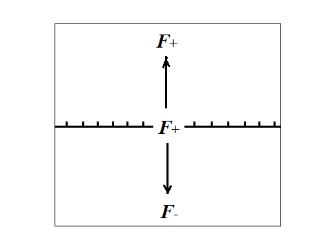
Figure 1. The singular support of a sheaf and the combinatoric description.

Proposition 3.7 (microlocal Morse inequality, [KS]*Proposition 5.4.20).

Let $\mathscr{F}\in Sh^{b}(M)$ and $f:M\rightarrow\mathbb{R}$ be a smooth function that is proper on $\mathrm{supp}(\mathscr{F})$. Let $\Lambda_{\varphi}=\{(x,d\varphi(x))|x\in M\}$, and suppose that

$$SS(\mathscr{F})\cap\Lambda_{\varphi}=\{(x_{1},\xi_{1}),...,(x_{n},\xi_{n})\}$$

and $V_{i}=\Gamma_{\varphi\geq\varphi(x_{i})}(\mathscr{F})_{x_{i}}$ is finite dimensional. Then $\Gamma(M,\mathscr{F})$ is also finite dimensional and for any $l\in\mathbb{Z}$

$$\sum_{1\leq i\leq n}\sum_{j\leq l}(-1)^{l-j}\dim H^{j}(V_{i})\geq\sum_{j\leq l}(-1)^{l-j}\dim H^{j}(M,\mathscr{F}).$$

In particular for any $j\in\mathbb{Z}$, $\sum_{1\leq i\leq n}\dim H^{j}(V_{i})\geq\dim H^{j}(M,\mathscr{F})$.

3.2. Microlocalization and $\mu Sh$

We review the definition and properties of microlocalization and the sheaf of categories $\mu Sh$. This will mainly used in the proof of the exact triangle (Theorem 1.7).

Definition 3.5.

Let $\Lambda\subset T^{*,\infty}M$ be a subset, $Sh^{b}_{(\Lambda)}(M)$ be the subcategory of sheaves $\mathscr{F}$ such that for some neighbourhood $\Lambda^{\prime}$ of $\Lambda$, $SS^{\infty}(\mathscr{F})\cap\Lambda^{\prime}\subset\Lambda.$ Then let a presheaf of dg categories on $\Lambda$ be

$$\mu Sh^{b,\text{pre}}_{\Lambda}:\,U\mapsto Sh^{b}_{(\Lambda)}(M)/Sh^{b}_{T^{*,\infty}M\backslash U}(M).$$

The sheafification of $\mu Sh^{b,\text{pre}}_{\Lambda}$ is $\mu Sh^{b}_{\Lambda}$. In particular, write $\mu Sh^{b}=\mu Sh_{T^{*,\infty}M}^{b}$ for the sheaf of categories on $T^{*,\infty}M$.

For $\mathscr{F,G}\in Sh^{b}(M)$, let the sheaf of homomorphisms in $\mu Sh^{b}_{\Lambda}$ be

$$\mu hom(\mathscr{F},\mathscr{G})|_{\Lambda}:\,U\mapsto Hom_{\mu Sh^{b}_{\Lambda}}(\mathscr{F,G}).$$

In particular, write $\mu hom(\mathscr{F},\mathscr{G})|_{T^{*,\infty}M}$ to be the sheaf of homomorphisms in $\mu Sh^{b}$.

Proposition 3.8 ([Gui]*Equation 6.4, [Guisurvey]*Equation 1.4.6).

For $p=(x,\xi)\in\Lambda\subset T^{*,\infty}M$ where $\Lambda\subset T^{*,\infty}M$ is a Legendrian, the stalk $\mu Sh^{b}_{p}$ satisfies the following: for $\mathscr{F,G}\in Sh_{(\Lambda)}^{b}(M)$, $\varphi\in C^{1}(M)$ such that $\varphi(x)=0,d\varphi(x)=\xi$,

$$Hom_{\mu Sh^{b}_{p}}(\mathscr{F,G})=\mu hom(\mathscr{F,G})_{p}=Hom(\Gamma_{\varphi\geq 0}(\mathscr{F})_{x},\Gamma_{\varphi\geq 0}(\mathscr{G})_{x}).$$

Theorem 3.9 ([Gui]*Proposition 6.6 & Lemma 6.7, [NadShen]*Corollary 5.4).

For $p=(x,\xi)\in\Lambda\subset T^{*,\infty}M$, the stalk $\mu Sh^{b}_{\Lambda,p}\simeq\mathrm{Perf}(\Bbbk)$.

Theorem 3.10 (Guillermou, [Gui]*Theorem 11.5).

Let $\Lambda\subset T^{*,\infty}M$ be a Legendrian submanifold. Suppose the Maslov class $\mu(\Lambda)=0$ and $\Lambda$ is relative spin, then as sheaves of categories

$$m_{\Lambda}:\,\mu Sh^{b}_{\Lambda}\xrightarrow{\sim}Loc^{b}_{\Lambda}.$$

Proposition 3.11 (Guillermou, [Gui]*Theorem 7.6 (iv), 7.9, 8.10 & Lemma 11.4).

Let $\Lambda\subset T^{*,\infty}M$ be a Legendrian submanifold. Suppose the Maslov class $\mu(\Lambda)=0$ and $\Lambda$ is relative spin. When the front projection of $\Lambda$ is a smooth hypersurface near $p$ and $\varphi\in C^{1}(M)$ is a local defining function for $\Lambda$, then

$$m_{\Lambda,p}(\mathscr{F})=\Gamma_{\varphi\geq 0}(\mathscr{F})_{x}[-d(p)].$$

For two different points $p$ and $p^{\prime}\in\Lambda$, $d(p)-d(p^{\prime})$ is equal to the difference of any Maslov potential at $p$ and $p^{\prime}$.

Example 3.6.

Suppose $\Lambda=\nu^{*,\infty}_{\mathbb{R}^{n}\times\mathbb{R}_{>0},-}\mathbb{R}^{n+1}\subset T^{*,\infty}\mathbb{R}^{n+1}$ is the inward conormal of $\mathbb{R}^{n}\times\mathbb{R}_{>0}$ and $\mathscr{F}\in Sh^{b}_{\Lambda}(\mathbb{R}^{n+1})$. Then $\mathscr{F}$ is determined by

For $p=(0,...,0,0;0,...,0,1)\in\Lambda$ we can pick $\varphi(x)=x_{n+1}$ and get

$$\Gamma_{\varphi\geq 0}(\mathscr{F})_{(0,...,0)}=\mathrm{Cone}(F_{+}\rightarrow F_{-})[-1]\simeq\mathrm{Tot}(F_{+}\rightarrow F_{-}).$$

Therefore one can see that the definition of the microstalk coincides with the definition of the microlocal monodromy defined by Shende-Treumann-Zaslow [STZ, Section 5.1], and indeed

$$m_{\Lambda,p}(\mathscr{F})\simeq\mu mon(\mathscr{F})_{p}[-1].$$

Now we are able to define the notion of microstalks, and thus define simple sheaves and pure sheaves, or microlocal rank $r$ sheaves.

Definition 3.6.

Let $\Lambda\subset T^{*,\infty}M$ be a Legendrian submanifold. Suppose $\mu(\Lambda)=0$ and $\Lambda$ is relative spin. For $p=(x,\xi)\in\Lambda$, the microstalk of $\mathscr{F}\in Sh^{b}(M)$ at $p$ is

$$m_{\Lambda,p}(\mathscr{F})=m_{\Lambda}(\mathscr{F})_{p}.$$

$\mathscr{F}\in Sh^{b}_{\Lambda}(M)$ is called microlocal rank $r$ if $m_{\Lambda,p}(\mathscr{F})$ is concentrated at a single degree with rank $r$. In this case $\mathscr{F}$ is called pure, and when $r=1$ it is also called simple.

Proposition 3.12 ([Guisurvey]*Equation 1.4.4).

Let $\Lambda\subset T^{*,\infty}M$ be a Legendrian submanifold. $\mathscr{F}\in Sh^{b}_{\Lambda}(M)$ is microlocal rank $r$ at $p\in\Lambda$ iff

$$\mu hom(\mathscr{F,F})_{p}\simeq\Bbbk^{r^{2}}.$$

Finally we recall the famous Sato’s exact triangle, which will be the essential ingredient for the proof of exact triangle in Theorem 1.7.

Theorem 3.13 (Sato’s exact triangle, [Gui]*Equation 2.17, [Guisurvey]*Equation 1.3.5).

Let $\mathscr{F}\in Sh^{b}(M)$ be a constructible sheaf. Then there is an exact triangle

$$D^{\prime}\mathscr{F}\otimes\mathscr{G}\rightarrow Hom(\mathscr{F,G})\rightarrow\pi_{*}(\mu hom(\mathscr{F,G})|_{T^{*,\infty}M})\xrightarrow{+1}.$$

3.3. Functors for Hamiltonian Isotopies

In this section we review the equivalence functor from a Hamiltonian isotopy defined by Guillermou-Kashiwara-Schapira [GKS].

Definition 3.7.

Let $\widehat{H}_{s}:T^{*}M\times I\rightarrow T^{*}M$ be a homogeneous Hamiltonian on $T^{*}M$. Then the Lagrangian graph of the Hamiltonian isotopy $\varphi_{\widehat{H}}^{s}\,(s\in I)$ is

$$\mathrm{Graph}_{\widehat{H}}=\{(x,x^{\prime},\xi,\xi^{\prime},s,\sigma)|(x^{\prime},\xi^{\prime})=\varphi_{\widehat{H}}^{s}(x,\xi),\sigma=-\widehat{H}_{s}\circ\varphi_{\widehat{H}}^{s}(x,\xi)\}\subset T^{*}(M\times M\times I).$$

For a conical Lagrangian $\widehat{\Lambda}$, the Lagrangian movie of $\widehat{\Lambda}$ under the Hamiltonian isotopy $\varphi_{\widehat{H}}^{s}\,(s\in I)$ is

$$\widehat{\Lambda}_{\widehat{H}}=\{(x,\xi,s,\sigma)|(x,\xi)=\varphi_{\widehat{H}}^{s}(x_{0},\xi_{0}),\sigma=-\widehat{H}_{s}\circ\varphi_{\widehat{H}}^{s}(x_{0},\xi_{0}),(x_{0},\xi_{0})\in\widehat{\Lambda}\}\subset T^{*}(M\times I).$$

Theorem 3.14 (Guillermou-Kashiwara-Schapira, [GKS]*Proposition 3.12).

Let $\widehat{H}_{s}:T^{*}M\times I\rightarrow T^{*}M$ be a homogeneous Hamiltonian on $T^{*}M$ and $\widehat{\Lambda}$ a conical Lagrangian in $T^{*}M$. Then there are functors that give equivalences

$$Sh_{\widehat{\Lambda}}(M)\xleftarrow{\sim}Sh_{\hat{\Lambda}_{\hat{H}}}(M\times I)\xrightarrow{\sim}Sh_{\varphi_{\widehat{H}}^{1}(\widehat{\Lambda})}(M)$$

given by restriction functors $i_{0}^{-1}$ and $i_{1}^{-1}$ where $i_{s}:M\times\{s\}\hookrightarrow M\times I$ is the inclusion.

4. Duality and Exact Triangle

4.1. Two Sheaf Categories

We recall the definitions we made in the introduction and prove some basic properties. As is explained in the introduction, we consider to add an extra $\mathbb{R}$ factor in order to see the Reeb chords. We follow the construction of Shende, which goes back to Tamarkin [Tamarkin1, Chapter 3]. Similar constructions can also been found in Guillermou [Gui, Section 13 & 16], Nadler-Shende [NadShen, Section 6] and Kuo [Kuo].

Definition 4.1 (Definition 1.2).

Let $q:M\times\mathbb{R}^{2}\rightarrow M\times\mathbb{R}$ be $q(x,t,u)=(x,t)$ and $r:M\times\mathbb{R}^{2}\rightarrow M\times\mathbb{R}$ be $r(x,t,u)=(x,t-u)$. For a Legendrian submanifold $\Lambda\subset T^{*,\infty}_{\tau>0}(M\times\mathbb{R})$, let

$$\begin{split}\Lambda_{q}&=\{(x,\xi,t,\tau,u,0)|(x,\xi,t,\tau)\in\Lambda\},\\ \Lambda_{r}&=\{(x,\xi,t+u,\tau,u,-\tau)|(x,\xi,t,\tau\in\Lambda)\}.\end{split}$$

For a sheaf $\mathscr{F}\in Sh^{b}(M\times\mathbb{R})$, let

$$\mathscr{F}_{q}=q^{-1}\mathscr{F},\,\,\,\mathscr{F}_{r}=r^{-1}\mathscr{F}.$$

Here, $\Lambda_{q}$ is the movie of $\Lambda$ under the identity contact isotopy, while $\Lambda_{r}$ is the movie of $\Lambda$ under the vertical translation defined by the Reeb flow. It is not hard to observe that every intersection point for some $\Lambda$ and Reeb translation $T_{c}(\Lambda)$ where

$$T_{c}:T^{*,\infty}_{\tau>0}(M\times\mathbb{R})\rightarrow T^{*,\infty}_{\tau>0}(M\times\mathbb{R});\,\,\,(x,\xi,t,\tau)\mapsto(x,\xi,t+c,\tau)$$

comes from a Reeb chord of $\Lambda$. The following lemma shows that those are all covectors pointing toward $du$ direction (i.e. in $M\times\mathbb{R}_{t}\times T^{*}\mathbb{R}_{u}$) that lie in the singular support of $\mathscr{H}om(\mathscr{F}_{q},\mathscr{G}_{r})$.

Lemma 4.1.

For $\Lambda\subset T^{*,\infty}_{\tau>0}(M\times\mathbb{R})$ and $\mathscr{F,G}\in Sh^{b}_{\Lambda}(M\times\mathbb{R})$,

$$SS^{\infty}(\mathscr{H}om(\mathscr{F}_{q},\mathscr{G}_{r}))\cap\mathrm{Graph}(du)=\emptyset.$$

On the other hand, there is an injection from

$$SS^{\infty}(\mathscr{H}om(\mathscr{F}_{q},\mathscr{G}_{r}))\cap\mathrm{Graph}(-du)$$

to the set of ordered Reeb chords (meaning the length $u$ can be positive or negative) $\mathcal{Q}_{\pm}(\Lambda)=\{\gamma:[0,u]\rightarrow T^{*,\infty}_{\tau>0}(M\times\mathbb{R})\,|\,\gamma(s)=(x,\xi,t+s,\tau),\,\gamma(0),\gamma(u)\in\Lambda\}$.

Proof.

Note that $\Lambda_{q}=\{(x,\xi,t,\tau,u,0)|(x,\xi,t,\tau)\in\Lambda\},\Lambda_{r}=\{(x,\xi,t+u,\tau,u,-\tau)|(x,\xi,t,\tau\in\Lambda)\}$. Since $SS^{\infty}(\mathscr{F}_{q})\cap SS^{\infty}(\mathscr{F}_{r})=\Lambda_{q}\cap\Lambda_{r}=\emptyset$, we can apply the singular support estimate Proposition 3.5

$$SS^{\infty}(\mathscr{H}om(\mathscr{F}_{r},\mathscr{G}_{q}))\subset(-SS^{\infty}(\mathscr{F}_{r}))+SS^{\infty}(\mathscr{G}_{q})=(-\Lambda_{r})+\Lambda_{q}.$$

Hence $(x,0,t,0,u,\nu)\in(-\Lambda_{q})+\Lambda_{r}$ iff there exists a pair $(x,\xi,t,\tau),(x,\xi,t+u,\tau)\in\Lambda$, or in other words there is a Reeb chord on $\Lambda$ of length $u$. In particular, we know that $\nu=-\tau<0$ is determined by such a pair. Hence when $\nu>0$, there will never be $(x,0,t,0,u,\nu)\in(-\Lambda_{q})+\Lambda_{r}$. Therefore

$$\begin{split}SS^{\infty}(\mathscr{H}om(\mathscr{F}_{q},\mathscr{G}_{r}&))\cap\mathrm{Graph}(du)=\emptyset\\ SS^{\infty}(\mathscr{H}om(\mathscr{F}_{q},\mathscr{G}_{r}))\,\cap&\,\mathrm{Graph}(-du)\hookrightarrow\mathcal{Q}_{\pm}(\Lambda)\end{split}$$

where our injection maps $(x,0,t,0,u,-\tau)$ to the Reeb chord connecting $(x,\xi,t,\tau),(x,\xi,t+u,\tau)\in\Lambda$. ∎

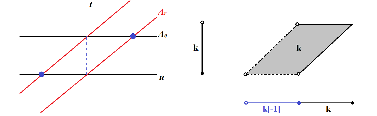
Figure 2. When $M$ is a point, $\Lambda\subset\mathbb{R}$ consists of two points $0$ and $1$, the front of the Legendrians $\Lambda_{q}$ and $\Lambda_{r}$ are shown on the left. For $\mathscr{F}=\Bbbk_{[0,1)}$, the sheaf $\mathscr{H}om(\mathscr{F}_{q},\mathscr{F}_{r})$ and its projection $u_{*}\mathscr{H}om(\mathscr{F}_{q},\mathscr{F}_{r})$ are shown on the right. The blue points are coming from the Reeb chord corresponding to the dashed blue line.

The following corollary produces an acyclic complex, which will be used to deduce Sabloff duality. The reader may compare it to the acyclic complex produced in generating family (co)homology [Genfamily, Section 3.1].

Corollary 4.2.

For $\Lambda\subset T^{*,\infty}_{\tau>0}(M\times\mathbb{R})$ and $\mathscr{F,G}\in Sh^{b}_{\Lambda}(M\times\mathbb{R})$ such that $\mathrm{supp}(\mathscr{F}),\mathrm{supp}(\mathscr{G})$ are compact,

$$\Gamma(M\times\mathbb{R}^{2},\mathscr{H}om(\mathscr{F}_{q},\mathscr{G}_{r}))\simeq 0.$$

Proof.

Since $SS^{\infty}(\mathscr{F}_{q})\cap SS^{\infty}(\mathscr{G}_{r})=\Lambda_{q}\cap\Lambda_{r}=\emptyset$, by Proposition 3.5

$$\mathscr{H}om(\mathscr{F}_{q},\mathscr{G}_{r})\simeq D^{\prime}\mathscr{F}_{q}\otimes\mathscr{G}_{r}.$$

Since $\mathrm{supp}(\mathscr{F}),\mathrm{supp}(\mathscr{G})$ are compact, we know that for sufficiently large $c>0$, $T_{\pm c}(\Lambda)\cap\Lambda=\emptyset$. Hence for large $c>0$,

$$\mathrm{supp}(D^{\prime}\mathscr{F}_{q}\otimes\mathscr{G}_{r})\subset q^{-1}(\mathrm{supp}(\mathscr{F}))\cap r^{-1}(\mathrm{supp}(\mathscr{G}))\subset M\times[-c,c]^{2}.$$

Therefore consider the function $\varphi_{+}(x,t,u)=u$, $\varphi_{+}|_{\mathrm{supp}(R\mathscr{H}om(\mathscr{F}_{q},\mathscr{G}_{r}))}$ is proper and

$$SS(\mathscr{H}om(\mathscr{F}_{q},\mathscr{G}_{r}))\cap\mathrm{Graph}(d\varphi_{+})=\emptyset.$$

One can apply microlocal Morse lemma 3.6 and see that

$$\Gamma(M\times\mathbb{R}^{2},\mathscr{H}om(\mathscr{F}_{q},\mathscr{G}_{r}))\simeq\Gamma(M\times\mathbb{R}\times(-\infty,-c),\mathscr{H}om(\mathscr{F}_{q},\mathscr{G}_{r}))=0.$$

This completes the proof. ∎

Similar to the case in Legendrian contact homology, where people defines two $\mathcal{A}_{\infty}$-categories $\mathcal{A}ug_{-}$ and $\mathcal{A}ug_{+}$, here we also define two dg categories of sheaves. The idea comes from the definition of the generating family cohomology.

From now on, the projection $M\times\mathbb{R}^{2},\,(x,t,u)\mapsto u$ will be denoted by $u$.

Definition 4.2 (Definition 1.3).

For $\Lambda\subset T^{*,\infty}_{\tau>0}(M\times\mathbb{R})$ and $\mathscr{F,G}\in Sh^{b}_{\Lambda}(M\times\mathbb{R})$, let

$$\begin{split}Hom_{-}(\mathscr{F,G})=\Gamma(u^{-1}([0,+\infty)),Hom(\mathscr{F}_{q},\mathscr{G}_{r})),\\ Hom_{+}(\mathscr{F,G})=\Gamma(u^{-1}((0,+\infty)),Hom(\mathscr{F}_{q},\mathscr{G}_{r})).\end{split}$$

Example 4.1.

Let $M$ be a point, $\Lambda\subset\mathbb{R}$ consists of two points $0$ and $1$ (see Figure 2). For $\mathscr{F}=\Bbbk_{[0,1)}$, the sheaf

$$u_{*}\mathscr{H}om(\mathscr{F}_{q},\mathscr{F}_{r})\simeq\Bbbk_{(-1,0]}[-1]\oplus\Bbbk_{(0,1]}.$$

Therefore as the projection $u:\mathbb{R}^{2}\rightarrow\mathbb{R}$ is proper on $\mathrm{supp}(\mathscr{H}om(\mathscr{F}_{q},\mathscr{F}_{r}))$, we have

$$\begin{split}Hom_{-}(\mathscr{F,F})=\Gamma([0,+\infty),\Bbbk_{0}[-1]&\oplus\Bbbk_{(0,1]})=\Bbbk[-1],\\ Hom_{+}(\mathscr{F,F})=\Gamma((0,+\infty),&\Bbbk_{(0,1]})=\Bbbk.\end{split}$$

Now we prove Theorem 1.8. The first part of the proof

$$\Gamma(u^{-1}((0,+\infty)),Hom(\mathscr{F}_{q},\mathscr{G}_{r}))\simeq Hom(\mathscr{F},\mathscr{G})$$

is essentially due to Guillermou [Gui, Corollary 16.6]. Here we adapt the proof of Jin-Treumann [JinTreu, Proposition 3.16].

Proof of Theorem 1.8 part 1: $Hom_{+}(\mathscr{F,G})\simeq Hom(\mathscr{F},\mathscr{G})$.

Let $C$ be the minimal length of chords $\gamma\in\mathcal{Q}(\Lambda)$. As in the proof of Corollary 4.2, we can choose $\varphi_{+}(x,t,u)=u$, and by microlocal Morse lemma 3.6, when $c_{0}<C$,

$$\Gamma(M\times\mathbb{R}\times(0,c_{0}),\mathscr{H}om(\mathscr{F}_{q},\mathscr{G}_{r}))\simeq\Gamma(M\times\mathbb{R}\times(0,+\infty),\mathscr{H}om(\mathscr{F}_{q},\mathscr{G}_{r})).$$

Now it suffices to show that

$$\Gamma(M\times\mathbb{R}\times(0,c_{0}),\mathscr{H}om(\mathscr{F}_{q},\mathscr{G}_{r}))\simeq Hom(\mathscr{F,G}).$$

This follows from Guillermou’s result which we now recall. Note that when $0<c<c_{0}$ there are no intersection points between $\Lambda$ and $T_{c}(\Lambda)$. Hence $(\Lambda_{q}\cup\Lambda_{r})\cap T^{*,\infty}(M\times\mathbb{R}\times(0,c))$ is the movie of a Legendrian isotopy (one can consider a Hamiltonian supported away from a neighbourhood of $\Lambda$ that is equal to $1$ near $\bigcup_{\epsilon<c<c_{0}}T_{c}(\Lambda)$). By Guillermou-Kashiwara-Schapira’s Theorem 3.14, we know for any $0<c<c_{0}$

$$\begin{split}\Gamma(M\times\mathbb{R}\times(0,c_{0}),\mathscr{H}om(\mathscr{F}_{q},\mathscr{G}_{r}))&\simeq Hom\Big{(}\varprojlim_{c>0}i^{-1}_{u=c}\mathscr{F}_{q},\varprojlim_{c>0}i^{-1}_{u=c}\mathscr{G}_{r}\Big{)}\\ &\simeq Hom\Big{(}\mathscr{F},\varprojlim_{c>0}T_{c,*}\mathscr{G}\Big{)}.\end{split}$$

Here $i_{u=c}:u^{-1}(c)\hookrightarrow M\times\mathbb{R}^{2}$ is the inclusion and $T_{c}:M\times\mathbb{R}\rightarrow M\times\mathbb{R}$ is the vertical translation (by abuse of notations). Note that since $SS^{\infty}(\mathscr{F}),SS^{\infty}(\mathscr{G})\subset T^{*,\infty}_{\tau>0}(M\times\mathbb{R})$, by microlocal cutoff lemma 3.2

$$\mathscr{G}\simeq\Bbbk_{[0,+\infty)}\star\mathscr{G}=s_{*}(\pi_{\mathbb{R}}^{-1}\Bbbk_{[0,+\infty)}\otimes\pi_{M\times\mathbb{R}}^{-1}\mathscr{G}),$$

where $s:M\times\mathbb{R}^{2}\rightarrow M\times\mathbb{R},\,(x,t_{1},t_{2})\mapsto(x,t_{1}+t_{2})$. By elementary computation we know

$$T_{c,*}\mathscr{G}\simeq\Bbbk_{[c,+\infty)}\star\mathscr{G},$$

and the map $\mathscr{G}\rightarrow T_{c,*}\mathscr{G}$ is induced by $\Bbbk_{[0,+\infty)}\rightarrow\Bbbk_{[c,+\infty)}$. Since $\Bbbk_{[0,+\infty)}\xrightarrow{\sim}\varprojlim_{c>0}\Bbbk_{[c,+\infty)}$, and the push-forward functor commutes with limits (which means that we can put the limit inside the convolution, i.e. $\varprojlim_{c>0}\big{(}\Bbbk_{[c,+\infty)}\star\mathscr{G}\big{)}\simeq\big{(}\varprojlim_{c>0}\Bbbk_{[c,+\infty)}\big{)}\star\mathscr{G}$), we can conclude that

$$Hom\Big{(}\mathscr{F},\varprojlim_{c>0}T_{c,*}\mathscr{G}\Big{)}\simeq Hom(\mathscr{F,G}).$$

This proves the assertion. ∎

For the second part of the theorem, we will need to use the fact that $\mathscr{H}om(\mathscr{F}_{q},\mathscr{G}_{r})\simeq D^{\prime}\mathscr{F}_{q}\otimes\mathscr{G}_{r}$ in order to relate $\mathscr{H}om(\mathscr{F}_{q},\mathscr{G}_{r})$ with $D^{\prime}\mathscr{F}\otimes\mathscr{G}$.

Proof of Theorem 1.8 part 2: $Hom_{-}(\mathscr{F,G})\simeq\Gamma(D^{\prime}\mathscr{F}\otimes\mathscr{G})$.

First of all note that for sufficiently small $\epsilon>0$, there are no Reeb chords of length less than $\epsilon$, in order words (by Lemma 4.1), no points in $((-\Lambda_{q})+\Lambda_{r})\cap\mathrm{Graph}(-du)$. Hence applying microlocal Morse lemma 3.6 to $u^{-1}((-\epsilon,+\infty))$ and $u^{-1}([0,+\infty))$ we know

$$\begin{split}\Gamma(u^{-1}([0,+\infty)),\mathscr{H}om(\mathscr{F}_{q},\mathscr{G}_{r}))&\simeq\varprojlim_{\epsilon>0}\Gamma(u^{-1}((-\epsilon,+\infty)),\mathscr{H}om(\mathscr{F}_{q},\mathscr{G}_{r}))\\ &\simeq\varprojlim_{\epsilon>0}\Gamma(u^{-1}((-\epsilon,+\infty)),\mathscr{H}om(i_{u>-\epsilon}^{-1}\mathscr{F}_{q},i_{u>-\epsilon}^{-1}\mathscr{G}_{r}))\end{split}$$

where $i_{u>-\epsilon}:u^{-1}((-\epsilon,+\infty))\hookrightarrow M\times\mathbb{R}^{2}$ is the inclusion. Second, by Lemma 4.1 we can again apply microlocal Morse lemma 3.6 and get

$$\begin{split}\Gamma(u^{-1}([0,+\infty)),\mathscr{H}om(\mathscr{F}_{q},\mathscr{G}_{r}))&\simeq\varprojlim_{\epsilon>0}\Gamma(u^{-1}((-\epsilon,\epsilon)),\mathscr{H}om(i_{u>-\epsilon}^{-1}\mathscr{F}_{q},i_{u>-\epsilon}^{-1}\mathscr{G}_{r}))\hskip 15.0pt\\ &\simeq\Gamma(u^{-1}(0),\mathscr{H}om(i_{u\geq 0}^{-1}\mathscr{F}_{q},i_{u\geq 0}^{-1}\mathscr{G}_{r}))\\ &\simeq\Gamma(u^{-1}(0),i_{u\geq 0}^{-1}(D^{\prime}\mathscr{F}_{q})\otimes i_{u\geq 0}^{-1}\mathscr{G}_{r}),\end{split}$$

where $i_{u\geq 0}:u^{-1}([0,+\infty))\hookrightarrow M\times\mathbb{R}^{2}$ is the inclusion. Note that by Proposition 3.5, we know $SS^{\infty}(\mathscr{H}om(\mathscr{F}_{q}|_{u\geq 0},\Bbbk|_{u\geq 0})))\cap\mathrm{Graph}(\pm du)=\emptyset$, so by microlocal Morse lemma

$$\begin{split}\Gamma(u^{-1}(0),D^{\prime}\mathscr{F}_{q}|_{u\geq 0})&=\Gamma(u^{-1}(0),\mathscr{H}om(i_{u\geq 0}^{-1}\mathscr{F}_{q},i_{u\geq 0}^{-1}\Bbbk_{M\times\mathbb{R}^{2}}))\\ &\simeq Hom(i_{u\geq 0}^{-1}\mathscr{F}_{q},i_{u\geq 0}^{-1}\Bbbk_{M\times\mathbb{R}^{2}})\\ &\simeq Hom(\mathscr{F},\Bbbk_{M\times\mathbb{R}})=\Gamma(D^{\prime}\mathscr{F}).\end{split}$$

Note that this is also true when we restrict to any open subset $U\subset u^{-1}(0)$ and $U\times[0,+\infty)\subset u^{-1}([0,+\infty))$, in other words we have $i_{u\geq 0}^{-1}(D^{\prime}\mathscr{F}_{q})\simeq D^{\prime}\mathscr{F}$. Therefore

$$\Gamma(u^{-1}([0,+\infty),\mathscr{H}om(\mathscr{F}_{q},\mathscr{G}_{r}))\simeq\Gamma(i_{u=0}^{-1}D^{\prime}\mathscr{F}_{q}\otimes i_{u=0}^{-1}\mathscr{G}_{r})\simeq\Gamma(D^{\prime}\mathscr{F}\otimes\mathscr{G}),$$

where $i_{u=0}:u^{-1}(0)\hookrightarrow M\times\mathbb{R}^{2}$ is the inclusion. The proof is completed. ∎

Remark 4.2.

The reason $Hom(\mathscr{F,G})\not\simeq Hom_{-}(\mathscr{F,G})$ is that for the homomorphism

$$i_{u=0}^{-1}\mathscr{H}om(\mathscr{F}_{q},\mathscr{G}_{r})\not\simeq\mathscr{H}om(i_{u=0}^{-1}\mathscr{F}_{q},i_{u=0}^{-1}\mathscr{G}_{r}).$$

(Using the language in Nadler-Shende [NadShen, Section 2], this is because the gapped condition fails for $\Lambda_{r}$ and $\Lambda_{q}$ as there exist Reeb chords whose lengths shrink to zero when $u\rightarrow 0$.) However, for tensor products we can easily get

$$i_{u=0}^{-1}(D^{\prime}\mathscr{F}\otimes\mathscr{G}_{r})\simeq i_{u=0}^{-1}(D^{\prime}\mathscr{F})\otimes i_{u=0}^{-1}\mathscr{G}.$$

4.2. Duality and Exact Triangle

Now we are able to prove Theorem 1.6 and 1.7.

Theorem 4.3 (Sabloff Duality; Theorem 1.6).

Let $M$ be orientable. For $\Lambda\subset T^{*,\infty}_{\tau>0}(M\times\mathbb{R})$ and $\mathscr{F,G}\in Sh^{b}_{\Lambda}(M\times\mathbb{R})$ with perfect stalk such that $\mathrm{supp}(\mathscr{F}),\mathrm{supp}(\mathscr{G})$ are compact,

$$\Gamma(u^{-1}((0,+\infty)),\mathscr{H}om(\mathscr{F}_{q},\mathscr{G}_{r}))\simeq D^{\prime}(\Gamma(u^{-1}([0,+\infty)),\mathscr{H}om(\mathscr{G}_{q},\mathscr{F}_{r})))[-n-1].$$

Before proving the theorem we use the acyclic complex obtained in Corollary 4.2 to get a partial duality result. Again one may compare the result with the analogous ones in generating families.

Proposition 4.4.

For $\Lambda\subset T^{*,\infty}_{\tau>0}(M\times\mathbb{R})$ and $\mathscr{F,G}\in Sh^{b}_{\Lambda}(M\times\mathbb{R})$ such that $\mathrm{supp}(\mathscr{F})$ and $\mathrm{supp}(\mathscr{G})$ are compact,

$$\Gamma(u^{-1}((0,+\infty)),\mathscr{H}om(\mathscr{F}_{q},\mathscr{G}_{r}))\simeq\Gamma_{u^{-1}((-\infty,0])}(M\times\mathbb{R}^{2},\mathscr{H}om(\mathscr{F}_{q},\mathscr{G}_{r})))[1].$$

Proof.

Consider the exact triangle

$$\Gamma_{u\leq 0}R\mathscr{H}om(\mathscr{F}_{r},\mathscr{G}_{q})\rightarrow\mathscr{H}om(\mathscr{F}_{r},\mathscr{G}_{q})\rightarrow i_{u>0,*}i_{u>0}^{-1}\mathscr{H}om(\mathscr{F}_{r},\mathscr{G}_{q})\xrightarrow{+1}.$$

Here $i_{u>0}:u^{-1}((0,+\infty))\hookrightarrow M\times\mathbb{R}^{2}$ is the inclusion. We have $\Gamma(M\times\mathbb{R}^{2},\mathscr{H}om(\mathscr{F}_{r},\mathscr{G}_{q}))\simeq 0$ by Corollary 4.2. Therefore the assertion follows. ∎

Proof of Theorem 4.3.

Since $\mathscr{F}_{r},\mathscr{G}_{q}$ are constructible, by Proposition 3.1 we have

$$\begin{split}\Gamma_{u\leq 0}(M\times\mathbb{R}^{2},\mathscr{H}om(\mathscr{F}_{q},\mathscr{G}_{r}))[1]&\simeq Hom(\Bbbk_{u\leq 0},\mathscr{H}om(\mathscr{F}_{q},\mathscr{G}_{r}))[1]\\ &\simeq Hom(\Bbbk_{u\leq 0},\mathscr{H}om(D\mathscr{G}_{r}\otimes\mathscr{F}_{q},\omega_{M\times\mathbb{R}^{2}}))[1]\\ &\simeq Hom(\Bbbk_{u\leq 0}\otimes(D\mathscr{G}_{r}\otimes\mathscr{F}_{q}),\omega_{M\times\mathbb{R}^{2}})[1]\end{split}$$

where $D(-)$ is the Verdier duality on $M\times\mathbb{R}^{2}$. Note that $M$ is orientable with dimension $n$, we have $D(-)=D^{\prime}(-)[n+2]$. Since $SS^{\infty}(\mathscr{F}_{q})\cap SS^{\infty}(\mathscr{G}_{r})=\emptyset$, we know $D^{\prime}\mathscr{G}_{r}\otimes\mathscr{F}_{q}\simeq\mathscr{H}om(\mathscr{G}_{r},\mathscr{F}_{q})$. Hence

$$\begin{split}Hom(D\mathscr{G}_{r}\otimes\mathscr{F}_{q}|_{u\leq 0},\omega_{M\times\mathbb{R}^{2}})[1]&\simeq Hom(\Gamma_{c}(M\times\mathbb{R}^{2},D^{\prime}\mathscr{G}_{r}\otimes\mathscr{F}_{q}|_{u\leq 0})[n+2],\Bbbk)[1]\\ &\simeq Hom(\Gamma_{c}(M\times\mathbb{R}^{2},\mathscr{H}om(\mathscr{G}_{r},\mathscr{F}_{q})|_{u\leq 0}),\Bbbk)[-n-1]\\ &\simeq D^{\prime}(\Gamma_{c}(M\times\mathbb{R}^{2},\mathscr{H}om(\mathscr{G}_{r},\mathscr{F}_{q})|_{u\leq 0}))[-n-1]\\ &\simeq D^{\prime}(\Gamma(M\times\mathbb{R}^{2},\mathscr{H}om(\mathscr{G}_{r},\mathscr{F}_{q})|_{u\leq 0}))[-n-1]\\ &\simeq D^{\prime}(\Gamma(u^{-1}((-\infty,0]),\mathscr{H}om(\mathscr{G}_{r},\mathscr{F}_{q})))[-n-1].\end{split}$$

The second last identity follows from the fact that the sheaf is compactly supported.

By reflection along the hyperplane $u=0$ and applying a Hamiltonian $H(x,t,u)=u$, i.e.

$$X_{H}=u\frac{\partial}{\partial t}-\frac{\partial}{\partial\nu},$$

$\Lambda_{r}\cap T^{*,\infty}(M\times\mathbb{R}\times(-\infty,0])$ (resp. $\Lambda_{q}\cap T^{*,\infty}(M\times\mathbb{R}\times(-\infty,0])$ is mapped to $\Lambda_{q}\cap T^{*,\infty}(M\times\mathbb{R}\times[0,+\infty))$ (resp. $\Lambda_{r}\cap T^{*,\infty}(M\times\mathbb{R}\times[0,+\infty))$. Thus by Guillermou-Kashiwara-Schapira’s Theorem 3.14 one can see that

$$\Gamma(u^{-1}((-\infty,0]),\mathscr{H}om(\mathscr{G}_{r},\mathscr{F}_{q}))\simeq\Gamma(u^{-1}([0,+\infty)),\mathscr{H}om(\mathscr{G}_{q},\mathscr{F}_{r})).$$

This completes the proof. ∎

Now we prove Thoerem 1.7. The main ingredient in the proof will be Sato’s exact triangle (Theorem 3.13).

Theorem 4.5 (Theorem 1.7; Sabloff-Sato exact triangle).

For $\Lambda\subset T^{*,\infty}_{\tau>0}(M\times\mathbb{R})$ a Legendrian, and $\mathscr{F}\in Sh^{b}_{\Lambda}(M\times\mathbb{R})$ a microlocal rank $r$ sheaf such that $\mathrm{supp}(\mathscr{F})$ is compact, we have an exact triangle

$$\Gamma(u^{-1}([0,+\infty)),\mathscr{H}om(\mathscr{F}_{q},\mathscr{F}_{r}))\rightarrow\Gamma(u^{-1}((0,+\infty)),\mathscr{H}om(\mathscr{F}_{q},\mathscr{F}_{r}))\rightarrow C^{*}(\Lambda;\Bbbk^{r^{2}})\xrightarrow{+1}.$$

Proof.

Consider Sato’s exact triangle 3.13

$$D^{\prime}\mathscr{F}\otimes\mathscr{F}\rightarrow\mathscr{H}om(\mathscr{F,F})\rightarrow\pi_{*}(\mu hom(\mathscr{F,F})|_{T^{*,\infty}(M\times\mathbb{R})})\xrightarrow{+1},$$

where $\pi:T^{*,\infty}(M\times\mathbb{R})\rightarrow M\times\mathbb{R}$ is the projection. We know by Theorem 3.10 that $\mu hom(\mathscr{F,F})|_{\dot{T}^{*}(M\times\mathbb{R})}\simeq\Bbbk^{r^{2}}_{\Lambda}$. Therefore taking global sections gives the following exact triangle

$$\Gamma(D^{\prime}\mathscr{F}\otimes\mathscr{F})\rightarrow Hom(\mathscr{F,F})\rightarrow C^{*}(\Lambda;\Bbbk^{r^{2}})\xrightarrow{+1}.$$

To show the assertion of the theorem, we claim that there is a commutative diagram of exact triangles where vertical arrows are all quasi-isomorphisms given by Theorem 1.8

In order to check the diagram on global sections, it suffices to check the diagram locally. Since $\mathscr{F}_{q},\mathscr{F}_{r}$ are constructible, in small open neighbourhoods around a point the sections are quasi-isomorphic to the stalks. Without loss of generality, one can assume that $u^{-1}(0)$ is a point. We can thus choose a small neighbourhood $U_{u^{-1}(0)}$ of $u^{-1}(0)$ such that

$$\Gamma(U_{u^{-1}(0)},D^{\prime}\mathscr{F}_{q}\otimes\mathscr{F}_{r})\simeq\Gamma(U_{u^{-1}(0)},D^{\prime}\mathscr{F}_{q})\otimes\Gamma(U_{u^{-1}(0)},\mathscr{F}_{r}).$$

Let’s write down all the maps in the diagram. The left vertical arrow factors as

$$\begin{split}\Gamma(u^{-1}([0,+\infty)),\mathscr{H}om(\mathscr{F}_{q},\mathscr{F}_{r}))&\rightarrow\Gamma(u^{-1}(0),\mathscr{H}om(\mathscr{F}_{q},\mathscr{F}_{r}))\\ &\leftarrow\Gamma(u^{-1}(0),D^{\prime}\mathscr{F}_{q}\otimes\mathscr{F}_{r})\rightarrow\Gamma(D^{\prime}\mathscr{F}\otimes\mathscr{F}_{r}).\end{split}$$

Pick $f_{0}^{\vee}\otimes f_{1}\in\Gamma(u^{-1}(0),D^{\prime}\mathscr{F}_{q}\otimes\mathscr{F}_{r})$. Viewing it as an element in $\Gamma(u^{-1}(0),\mathscr{H}om(\mathscr{F}_{q},\mathscr{F}_{r}))$, there is a cohomologous element $\bar{f}_{0}^{\vee}\otimes\bar{f}_{1}\in\Gamma(u^{-1}([0,+\infty)),\mathscr{H}om(\mathscr{F}_{q},\mathscr{F}_{r}))$. On the other hand, the image of $f_{0}^{\vee}\otimes f_{1}$ in $\Gamma(D^{\prime}\mathscr{F}\otimes\mathscr{F})$ will be $i_{u=0}^{-1}f_{0}^{\vee}\otimes i_{u=0}^{-1}f_{1}$.

Under the bottom horizontal map, the image of $\bar{f}_{0}^{\vee}\otimes\bar{f}_{1}$ will be $i_{u>0}^{-1}\bar{f}_{0}^{\vee}\otimes i_{u>0}^{-1}\bar{f}_{1}$, and under the top horizontal map, the image of $i_{u=0}^{-1}f_{0}^{\vee}\otimes i_{u=0}^{-1}f_{1}$ can be denoted again by $i_{u=0}^{-1}f_{0}^{\vee}\otimes i_{u=0}^{-1}f_{1}$. Note that the right vertical arrow factors as

$$\begin{split}\Gamma(u^{-1}((0,+\infty)),\mathscr{H}om(\mathscr{F}_{q},\mathscr{F}_{r}))&\rightarrow\Gamma(u^{-1}((0,c_{0})),\mathscr{H}om(\mathscr{F}_{q},\mathscr{F}_{r}))\\ &\rightarrow Hom(\mathscr{F},T_{c,*}\mathscr{F})\rightarrow Hom(\mathscr{F},\Bbbk_{[c,+\infty)}\star\mathscr{F})\\ &\leftarrow Hom(\mathscr{F},\Bbbk_{[0,+\infty)}\star\mathscr{F})\rightarrow Hom(\mathscr{F,F}).\end{split}$$

Hence $i_{u>0}^{-1}\bar{f}_{0}^{\vee}\otimes i_{u>0}^{-1}\bar{f}_{1}$ will be mapped to $i_{u=c}^{-1}\bar{f}_{0}^{\vee}\otimes i_{u=c}^{-1}\bar{f}_{1}$ and then to $i_{u=c}^{-1}\bar{f}_{0}^{\vee}\otimes T_{c}^{-1}i_{u=c}^{-1}\bar{f}_{1}$.

Since $q^{-1}$ and $r^{-1}$ are equivalences by Theorem 3.14, we may assume that $\bar{f}_{0}^{\vee}=q^{-1}(f^{\prime}_{0})^{\vee}$, $\bar{f}_{1}^{\vee}=r^{-1}f^{\prime}_{1}$ and $f_{0}^{\vee}=q_{U_{u^{-1}(0)}}^{-1}(f^{\prime\prime}_{0})^{\vee},f_{1}^{\vee}=r_{U_{u^{-1}(0)}}^{-1}f^{\prime\prime}_{1}$. Hence

$$i_{u=0}^{-1}f_{0}^{\vee}\otimes i_{u=0}^{-1}f_{1}=i_{u=0}^{-1}q^{-1}(f^{\prime\prime}_{0})^{\vee}\otimes i_{u=0}^{-1}r^{-1}f^{\prime\prime}_{1}=(f^{\prime\prime}_{0})^{\vee}\otimes f^{\prime\prime}_{1}.$$

Note that $i_{u=c}^{-1}q^{-1}=\mathrm{id}$, so

$$i_{u=c}^{-1}\bar{f}_{0}^{\vee}=i_{u=c}^{-1}q^{-1}(f^{\prime}_{0})^{\vee}=(f^{\prime}_{0})^{\vee}.$$

On the other hand, note that $i_{u=c}^{-1}r^{-1}=T_{c,*}$, we have

$$T_{c}^{-1}i_{u=c}^{-1}\bar{f}_{1}=T_{c}^{-1}i_{u=c}^{-1}r^{-1}f^{\prime}_{1}=T_{c}^{-1}T_{c,*}f^{\prime}_{1}=f^{\prime}_{1}.$$

However, we know that $f_{0},\bar{f}_{0}|_{U_{u^{-1}(0)}}$ and $f_{0},\bar{f}_{1}|_{U_{u^{-1}(0)}}$ are cohomologous, so are $f^{\prime}_{0},f^{\prime\prime}_{0}$ and $f^{\prime}_{1},f^{\prime\prime}_{1}$. Thus the diagram commutes up to homotopy. ∎

The theorem can be easily generalized to the case when the sheaf $\mathscr{F}$ is not pure, but has perfect microstalk.

Theorem 4.6.

For $\Lambda\subset T^{*,\infty}_{\tau>0}(M\times\mathbb{R})$ a Legendrian, and $\mathscr{F}\in Sh^{b}_{\Lambda}(M\times\mathbb{R})$ a sheaf with perfect microstalk $F$ such that $\mathrm{supp}(\mathscr{F})$ is compact, we have an exact triangle

$$\begin{split}\Gamma(u^{-1}([0,+\infty)),\mathscr{H}om(\mathscr{F}_{q},\mathscr{F}_{r}))&\rightarrow\Gamma(u^{-1}((0,+\infty)),\mathscr{H}om(\mathscr{F}_{q},\mathscr{F}_{r}))\\ &\rightarrow C^{*}(\Lambda;Hom(F,F))\xrightarrow{+1}.\end{split}$$

Proof.

By our previous proof, it suffices to show that

$$\mu hom(\mathscr{F,F})|_{T^{*,\infty}(M\times\mathbb{R})}\simeq Hom(F,F)_{\Lambda}.$$

We know that $\mu hom(\mathscr{F,F})|_{T^{*,\infty}(M\times\mathbb{R})}\simeq\mu hom(\mathscr{F,F})|_{\Lambda}$ and the latter is a locally constant sheaf on $\Lambda$. By Guillermou’s Theorem 3.10, $\mu Sh^{b}_{\Lambda}(\Lambda)\simeq Loc^{b}_{\Lambda}(\Lambda)$. Thus

$$\Gamma(T^{*,\infty}(M\times\mathbb{R}),\mu hom(\mathscr{F,F})|_{\Lambda})\simeq Hom(m_{\Lambda}(\mathscr{F}),m_{\Lambda}(\mathscr{F}))\simeq Hom(F,F).$$

This completes the proof. ∎

The following corollary can be viewed as a version of degeneration to Morse flow trees in Legendrian contact homology (that certain pseudoholomorphic curves degenerate to Morse gradient flows) in for example [EESduality, Theorem 3.6, Part (4)]. It says that certain sheaf homomorphisms descend to Morse theory. A similar result in sheaf theory can also been found in [Ike, Section 4.3].

Corollary 4.7.

For $\Lambda\subset T^{*,\infty}_{\tau>0}(M\times\mathbb{R})$ and $\mathscr{F}\in Sh^{b}_{\Lambda}(M\times\mathbb{R})$ a microlocal rank $r$ sheaf such that $\mathrm{supp}(\mathscr{F})$ is compact, then

$$\Gamma(u^{-1}(0),\Gamma_{u\leq 0}(\mathscr{H}om(\mathscr{F}_{q},\mathscr{F}_{r})))[1]\simeq C^{*}(\Lambda;\Bbbk^{r^{2}}).$$

Proof.

Note that we have an exact triangle

$$\begin{split}i_{u\geq 0}^{-1}\mathscr{H}om(\mathscr{F}_{q},\mathscr{F}_{r})&\,\rightarrow i^{\prime}_{u>0,*}i_{u>0}^{-1}\mathscr{H}om(\mathscr{F}_{q},\mathscr{F}_{r})\\ &\,\rightarrow\Gamma_{u=0}(i_{u\geq 0}^{-1}\mathscr{H}om(\mathscr{F}_{q},\mathscr{F}_{r}))[1]\xrightarrow{+1}.\end{split}$$

Here $i_{u\geq 0}:u^{-1}([0,+\infty))\hookrightarrow M\times\mathbb{R}^{2}$ and $i^{\prime}_{u>0}:u^{-1}((0,+\infty))\hookrightarrow u^{-1}([0,+\infty))$ are the inclusions. Taking global sections and compare it with the exact triangle in Theorem 1.7, we know that

$$\Gamma_{u=0}(M\times\mathbb{R}^{2},i_{u\geq 0}^{-1}\mathscr{H}om(\mathscr{F}_{q},\mathscr{F}_{r}))[1]\simeq C^{*}(\Lambda;\Bbbk^{r^{2}}).$$

However, write $i_{u\geq-\epsilon}$ to be the inclusion $u^{-1}((-\epsilon,+\infty))\hookrightarrow M\times\mathbb{R}^{2}$. We also have

$$\begin{split}\Gamma_{u=0}(M\times\mathbb{R}^{2},i_{u\geq 0}^{-1}\mathscr{H}om(\mathscr{F}_{q},\mathscr{F}_{r}))&\simeq Hom(\Bbbk_{u=0},i_{u\geq 0}^{-1}\mathscr{H}om(\mathscr{F}_{q},\mathscr{F}_{r}))\\ &\simeq\varprojlim_{\epsilon>0}Hom(i_{u\geq-\epsilon}^{-1}\Bbbk_{u\leq 0},i_{u\geq-\epsilon}^{-1}\mathscr{H}om(\mathscr{F}_{q},\mathscr{F}_{r}))\end{split}$$

This isomorphism is because for sufficiently small $\epsilon>0$, there are no Reeb chords of length less than $\epsilon$, and thus (by Lemma 4.1), no points in $((-\Lambda_{q})+\Lambda_{r})\cap\mathrm{Graph}(-du)$. Therefore by microlocal Morse lemma the homomorphism on $u^{-1}([0,+\infty))$ is the same as $u^{-1}((-\epsilon,+\infty))$ for small $\epsilon>0$.

$$\begin{split}\Gamma_{u=0}(M\times\mathbb{R}^{2},i_{u\geq 0}^{-1}\mathscr{H}om(\mathscr{F}_{q},\mathscr{F}_{r}))&\simeq\varprojlim_{\epsilon>0}Hom(i_{u\geq-\epsilon}^{-1}\Bbbk_{u\leq 0},i_{u\geq-\epsilon}^{-1}\mathscr{H}om(\mathscr{F}_{q},\mathscr{F}_{r}))\\ &\simeq\varprojlim_{\epsilon>0}Hom(i_{|u|<\epsilon}^{-1}\Bbbk_{u\leq 0},i_{|u|<\epsilon}^{-1}\mathscr{H}om(\mathscr{F}_{q},\mathscr{F}_{r}))\\ &\simeq\varprojlim_{\epsilon>0}\Gamma(u^{-1}((-\epsilon,\epsilon)),\Gamma_{u\leq 0}(\mathscr{H}om(\mathscr{F}_{q},\mathscr{F}_{r})))\\ &\simeq\Gamma(u^{-1}(0),\Gamma_{u\leq 0}(\mathscr{H}om(\mathscr{F}_{q},\mathscr{F}_{r}))).\end{split}$$

Here $i_{|u|<\epsilon}:u^{-1}((-\epsilon,\epsilon))\hookrightarrow M\times\mathbb{R}^{2}$ is the inclusion. The second equality holds because Lemma 4.1 enables us to apply microlocal Morse lemma restrict from $u^{-1}((-\epsilon,+\infty))$ to $u^{-1}((-\epsilon,\epsilon))$. This proves our assertion. ∎

5. Persistence and Hamiltonian Isotopy

5.1. Persistence Modules and Sheaves

A persistent module is roughly speaking an $\mathbb{R}$-direct system of modules. It has been studied by a number of people, for example in [Proximitypersist, Stablepersist].

Definition 5.1.

Let $\Bbbk$ be a ring. A persistence module $M_{\mathbb{R}}$ is a family $\{M_{\alpha}\}_{\alpha\in\mathbb{R}}$ of graded $\Bbbk$-modules, together with a family $\{f_{\alpha_{0}\alpha_{1}}:M_{\alpha_{0}}\rightarrow M_{\alpha_{1}}\}_{\alpha_{0}\leq\alpha_{1}}$ such that $f_{\alpha_{1}\alpha_{2}}\circ f_{\alpha_{0}\alpha_{1}}=f_{\alpha_{0}\alpha_{2}}$ and $f_{\alpha\alpha}=\mathrm{id}_{M_{\alpha}}$. $M_{\mathbb{R}}$ is tame if for any $\alpha\in\mathbb{R}$, $\dim M_{\alpha}<\infty$.

Definition 5.2.

Let $M_{\mathbb{R}},N_{\mathbb{R}}$ be two persistence modules. They are $(\epsilon,\epsilon^{\prime})$-interleaved if there exists

$$\begin{split}\phi_{\alpha}:M_{\alpha}\rightarrow N_{\alpha+\epsilon},&\,\,\phi^{\prime}_{\alpha}:M_{\alpha}\rightarrow N_{\alpha+\epsilon^{\prime}},\\ \psi_{\alpha}:N_{\alpha}\rightarrow M_{\alpha+\epsilon},&\,\,\psi^{\prime}_{\alpha}:N_{\alpha}\rightarrow M_{\alpha+\epsilon^{\prime}}\end{split}$$

such that the following diagrams commute

$$f^{M}_{\alpha,\alpha+\epsilon+\epsilon^{\prime}}=\psi_{\alpha+\epsilon}\circ\phi_{\alpha},\,\,f^{N}_{\alpha,\alpha+\epsilon+\epsilon^{\prime}}=\phi^{\prime}_{\alpha+\epsilon^{\prime}}\circ\psi^{\prime}_{\alpha}.$$

The interleaving distance between $M_{\mathbb{R}},N_{\mathbb{R}}$ is

$$d(M_{\mathbb{R}},N_{\mathbb{R}})=\inf\{\epsilon+\epsilon^{\prime}|M_{\mathbb{R}},N_{\mathbb{R}}\text{ are }(\epsilon,\epsilon^{\prime})\text{-interleaved}\}.$$

One of the origins of the study of persistence modules is to study real functions on a manifold. Let $f\in C^{\infty}(X)$ and $X_{f}^{\alpha}=f^{-1}((\alpha,+\infty))$. Then $\{H^{*}(X_{f}^{\alpha})\}_{\alpha\in\mathbb{R}}$ is a persistence module. A crucial result in [Proximitypersist] is that the distance of a family of persistence modules $\{H^{*}(X_{f}^{\alpha})\}_{\alpha\in\mathbb{R}}$ when $f$ changes is controlled by the $C^{0}$-norm of $f$:

$$d(H^{*}(X_{f}^{\alpha}),H^{*}(X_{g}^{\alpha}))\leq d_{C^{0}}(f,g).$$

Remark 5.1.

In [Proximitypersist] the authors were assuming that $\phi=\psi,\phi^{\prime}=\psi^{\prime}$ and only got the bound by $2d_{C^{0}}(f,g)$. However, when Usher-Zhang [UsherZpersist], or Asano-Ike [AsanoIke] were trying to define an analogue of the interleaving distance and apply that to symplectic topology, they found that one had to allow the case where $\phi\neq\psi,\phi^{\prime}\neq\psi^{\prime}$ in order to get a better bound $d_{C^{0}}(f,g)$. Therefore we adapt their definition here.

In this paper, we will use the language of constructible sheaves on $\mathbb{R}$ instead of persistence modules. Here is the classification result of these sheaves.

Theorem 5.1 (Guillermou [Guithree]*Corollary 7.3; Kashiwara-Schapira [GS]*Theorem 1.17).

Let $\mathscr{F}\in Sh_{\nu<0}^{b}(\mathbb{R})$ be a constructible sheaf. Then there exists a finite (index) set $A$ such that

$$\mathscr{F}\simeq\bigoplus_{\alpha\in A}\Bbbk^{r_{\alpha}}_{(u_{\alpha},v_{\alpha}]}[n_{\alpha}].$$

Each interval $(u_{\alpha},v_{\alpha}]$ is called a bar.

Note that for any constructible sheaf $\mathscr{F}\in Sh_{\nu<0}^{b}(\mathbb{R})$, we can associate a tame persistence module by $M_{\alpha}=H^{*}\Gamma((-\infty,\alpha),\mathscr{F}).$ All definitions and results in persistence modules can be stated in 1-dimensional sheaf theory easily. In fact, one can probably show that the category of tame persistence modules is equivalent to the full subcategory of constructible sheaves in $Sh^{b}_{\nu<0}(\mathbb{R})$. However we won’t discuss it here.

Now we define the interleaving distance for sheaves in arbitrary dimensions.

Definition 5.3 (Asano-Ike, [AsanoIke]).

Let $\mathscr{F,G}\in Sh_{\tau>0}^{b}(M\times\mathbb{R})$ be two constructible sheaves. Let $T_{c}:\mathbb{R}\rightarrow\mathbb{R}$ be the translation $T_{c}(x,t)=(x,t+c)$. They are $(\epsilon,\epsilon^{\prime})$-interleaved if there exists

$$\begin{split}\phi:\mathscr{F}\rightarrow T_{\epsilon,*}\mathscr{G},&\,\,\psi:\mathscr{G}\rightarrow T_{\epsilon^{\prime},*}\mathscr{F},\\ \phi^{\prime}:\mathscr{G}\rightarrow T_{\epsilon,*}\mathscr{F},&\,\,\psi^{\prime}:\mathscr{F}\rightarrow T_{\epsilon^{\prime},*}\mathscr{G}\end{split}$$

such that the following diagrams commute

$$t^{\mathscr{F}}_{0,\epsilon+\epsilon^{\prime}}=T_{\epsilon,*}\psi\circ\phi,\,\,t^{\mathscr{G}}_{0,\epsilon+\epsilon^{\prime}}=T_{\epsilon^{\prime},*}\phi^{\prime}\circ\psi^{\prime}$$

where $t^{\mathscr{H}}_{a,b}:\mathscr{H}\rightarrow T_{a+b,*}\mathscr{H}$ is the natural map. The interleaving distance between $\mathscr{F,G}$ is

$$d(\mathscr{F,G})=\inf\{\epsilon+\epsilon^{\prime}|\mathscr{F,G}\text{ are }(\epsilon,\epsilon^{\prime})\text{-interleaved}\}.$$

Example 5.2.

Consider the sheaves $\Bbbk_{(a_{0},b_{0}]}$ and $\Bbbk_{(a_{1},b_{1}]}$ in $Sh_{\nu<0}^{b}(\mathbb{R})$. Since their singular supports satisfy $\nu<0$, we need to choose the translation in the negative direction $U_{c}:\mathbb{R}\rightarrow\mathbb{R},\,x\mapsto x-c$. Then if $a,a^{\prime},b,b^{\prime}$ are distinct, by Proposition 3.5

$$\mathscr{H}om(\Bbbk_{(a,b]},\Bbbk_{(a^{\prime},b^{\prime}]})=\Bbbk_{[a,b)\cap(a^{\prime},b^{\prime}]}.$$

There exists a degree zero non-vanishing map iff $a^{\prime}<a$ and $b^{\prime}<b$. Now we estimate the distance between $\Bbbk_{(a_{0},b_{0}]}$ and $\Bbbk_{(a_{1},b_{1}]}$ in two specific cases.

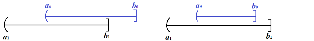
Figure 3. The sheaves $\Bbbk_{(a_{0},b_{0}]}$ and $\Bbbk_{(a_{1},b_{1}]}$ in two different cases.

Suppose $a_{0}>a_{1},b_{0}>b_{1}$ and $a_{0}<b_{1}$ (Figure 3 left). When $\epsilon+\epsilon^{\prime}>b_{1}-a_{1}$, the natural map

$$\tau_{0,\epsilon+\epsilon^{\prime}}:\Bbbk_{(a_{1},b_{1}]}\rightarrow\Bbbk_{(a_{1}-\epsilon-\epsilon^{\prime},b_{1}-\epsilon-\epsilon^{\prime}]}$$

becomes zero, so we can choose all the maps to be zero. Now we assume that $\epsilon+\epsilon^{\prime}<b_{1}-a_{1}$, which means the natural map as a composition

$$\tau_{0,\epsilon+\epsilon^{\prime}}:\Bbbk_{(a_{1},b_{1}]}\rightarrow\Bbbk_{(a_{0}-\epsilon^{\prime},b_{0}-\epsilon^{\prime}]}\rightarrow\Bbbk_{(a_{1}-\epsilon-\epsilon^{\prime},b_{1}-\epsilon-\epsilon^{\prime}]}$$

is nonzero. For the second map to be nonzero, we require $a_{0}-\epsilon^{\prime}<a_{1}$ and $b_{0}-\epsilon^{\prime}<b_{1}$, i.e. $\epsilon^{\prime}>\max\{a_{0}-a_{1},b_{0}-b_{1}\}$. Now we choose any

$$\epsilon>0,\,\,\,\epsilon^{\prime}>\max\{a_{0}-a_{1},b_{0}-b_{1}\}.$$

Then maps in the composition

$$\tau_{0,\epsilon+\epsilon^{\prime}}:\Bbbk_{(a_{1},b_{1}]}\rightarrow\Bbbk_{(a_{0}-\epsilon^{\prime},b_{0}-\epsilon^{\prime}]}\rightarrow\Bbbk_{(a_{1}-\epsilon-\epsilon^{\prime},b_{1}-\epsilon-\epsilon^{\prime}]}$$

can be chosen to be nonzero. For the other composition

$$\tau_{0,\epsilon+\epsilon^{\prime}}:\Bbbk_{(a_{0},b_{0}]}\rightarrow\Bbbk_{(a_{1}-\epsilon,b_{1}-\epsilon]}\rightarrow\Bbbk_{(a_{0}-\epsilon-\epsilon^{\prime},b_{0}-\epsilon-\epsilon^{\prime}]},$$

we have $a_{0}-\epsilon-\epsilon^{\prime}<a_{1}-\epsilon,b_{0}-\epsilon-\epsilon^{\prime}<b_{1}-\epsilon$. Therefore the maps can also be chosen to be nonzero. Therefore we can show that the distance is

$$d(\Bbbk_{(a_{0},b_{0}]},\Bbbk_{(a_{1},b_{1}]})=\inf\{\epsilon+\epsilon^{\prime}\}=\max\{a_{1}-a_{0},b_{1}-b_{0}\}.$$

Suppose $a_{0}>a_{1},b_{0}<b_{1}$. Then $(a_{0},b_{0}]\subset(a_{1},b_{1}]$ (Figure 3 right). Without loss of generality, we may still assume that $\epsilon+\epsilon^{\prime}<b_{1}-a_{1}$, which means the composition

$$\tau_{0,\epsilon+\epsilon^{\prime}}:\Bbbk_{(a_{1},b_{1}]}\rightarrow\Bbbk_{(a_{0}-\epsilon^{\prime},b_{0}-\epsilon^{\prime}]}\rightarrow\Bbbk_{(a_{1}-\epsilon-\epsilon^{\prime},b_{1}-\epsilon-\epsilon^{\prime}]}$$

is nonzero. For the first map to be nonzero, we require $a_{0}-\epsilon^{\prime}<a_{1}<b_{0}-\epsilon^{\prime}$, i.e. $\epsilon^{\prime}>a_{0}-a_{1}$. For the second map to be nonzero, we require $a_{0}-\epsilon^{\prime}<b_{1}-\epsilon-\epsilon^{\prime}<b_{0}-\epsilon^{\prime}$, i.e. $\epsilon>b_{1}-b_{0}$. Therefore one can show that

$$d(\Bbbk_{(a_{0},b_{0}]},\Bbbk_{(a_{1},b_{1}]})=\inf\{\epsilon+\epsilon^{\prime}\}=(a_{0}-a_{1})+(b_{1}-b_{0}).$$

For the other two cases, one has similar results. In conclusion, one can see that the persistence distance is measuring how far the bars differ from each other (in fact it is the Gromov-Hausdorff distance between the intervals).

Here is a basic property we’re going to use from time to time. It basically says that the persistence distance is a pseudo metric.

Lemma 5.2.

Suppose $\mathscr{F,G}$ are $(a_{0},b_{0})$-interleaved, and $\mathscr{G,H}$ are $(a_{1},b_{1})$-interleaved. Then $\mathscr{F,H}$ are $(a_{0}+a_{1},b_{0}+b_{1})$-interleaved. In particular,

$$d(\mathscr{F,H})\leq d(\mathscr{F,G})+d(\mathscr{G,H}).$$

Proof.

We have the following commutative diagrams that give the natural maps $\tau_{0,a_{0}+b_{0}}$ and $\tau_{0,a_{1}+b_{1}}$:

$$\begin{split}\mathscr{F}\xrightarrow{\phi}T_{a_{0},*}\mathscr{G}\xrightarrow{T_{a_{0},*}\psi}T_{a_{0}+b_{0},*}\mathscr{F},&\,\,\mathscr{G}\xrightarrow{\phi^{\prime}}T_{b_{0},*}\mathscr{F}\xrightarrow{T_{b_{0},*}\psi^{\prime}}T_{a_{0}+b_{0},*}\mathscr{G},\\ \mathscr{G}\xrightarrow{\gamma}T_{a_{1},*}\mathscr{H}\xrightarrow{T_{a_{0},*}\delta}T_{a_{1}+b_{1},*}\mathscr{G},&\,\,\mathscr{H}\xrightarrow{\gamma^{\prime}}T_{b_{1},*}\mathscr{G}\xrightarrow{T_{b_{0},*}\delta^{\prime}}T_{a_{1}+b_{1},*}\mathscr{H}.\end{split}$$

Therefore we can construct the following maps that give the natural map $\tau_{0,a_{0}+a_{1}+b_{0}+b_{1}}$:

$$\begin{split}\mathscr{F}\xrightarrow{T_{a_{0},*}\gamma\circ\phi}T_{a_{0}+a_{1},*}\mathscr{H}&\,\xrightarrow{T_{a_{0}+a_{1}+b_{1},*}\psi\circ T_{a_{0}+a_{1},*}\delta}T_{a_{0}+b_{0}+b_{0}+b_{1},*}\mathscr{F},\\ \mathscr{H}\xrightarrow{T_{a_{1},*}\phi^{\prime}\circ\gamma^{\prime}}T_{a_{1}+a_{0},*}\mathscr{F}&\,\xrightarrow{T_{a_{1}+a_{0}+b_{0},*}\delta^{\prime}\circ T_{a_{1}+a_{0},*}\psi^{\prime}}T_{a_{1}+a_{0}+b_{1}+b_{0},*}\mathscr{H}.\end{split}$$

This proves the assertion. ∎

5.2. Continuity under Hamiltonian Isotopy

Given a Hamiltonian isotopy $\varphi_{H}^{s}\,(s\in I)$ on $T^{*,\infty}_{\tau>0}(M\times\mathbb{R})$, Guillermou-Kashiwara-Schapira defined an equivalence functor called sheaf quantization $\Phi_{H}^{s}:Sh^{b}_{\tau>0}(M\times\mathbb{R})\rightarrow Sh^{b}_{\tau>0}(M\times\mathbb{R})$ (Theorem 3.14). Asano and Ike studied how the quantization of a Hamiltonian isotopy changes the interleaving distance. Recall that

$$\|H\|_{\text{osc}}=\int_{0}^{1}\left(\max H_{s}-\min H_{s}\right)\,ds.$$

Theorem 5.3 (Asano-Ike, [AsanoIke]).

Let $H$ be a compactly supported Hamiltonian on $T^{*,\infty}_{\tau>0}(M\times\mathbb{R})$ and $\Phi_{H}^{s}\,(s\in I)$ be its sheaf quantization functor. Then for $\mathscr{F}\in Sh_{\tau>0}^{b}(M\times\mathbb{R})$,

$$d(\mathscr{F},\Phi_{H}^{1}(\mathscr{F}))\leq\|H\|_{\text{osc}}.$$

To make the section self-contained, we give a proof of the theorem (the version we’re going to use is a little bit weaker as we will add the proper assumption in the following lemma, but that’s unnecessary). Denote by $\gamma_{a,b}$ the following cone in $\mathbb{R}^{2}$:

$$\gamma_{a,b}=\{(\tau,\sigma)|-a\tau<\sigma<b\tau\}\subset\mathbb{R}^{2}.$$

Lemma 5.4 (Guillermou-Schapira, [GS]*Proposition 5.9; [AsanoIke]*Proposition 4.3).

For $\mathscr{H}\in Sh_{\tau>0}^{b}(M\times\mathbb{R}\times I)$ and $s_{0}<s_{1}\in I$, if there exists $a,b,r\in\mathbb{R}_{>0}$ such that

$$SS(\mathscr{H})\cap T^{*}(M\times\mathbb{R}\times(s_{0}-r,s_{1}+r))\subset T^{*}M\times\left((\mathbb{R}\times I)\times\gamma_{a,b}\right),$$

Suppose the projection $\pi_{M\times\mathbb{R}}:M\times\mathbb{R}\times I\rightarrow M\times\mathbb{R}$ is proper on $\mathrm{supp}(\mathscr{H})$. Then the natural morphisms

$$\begin{split}\tau_{0,a(s_{1}-s_{0})+\epsilon}:&\,\pi_{M\times\mathbb{R},*}(\mathscr{H}|_{M\times\mathbb{R}\times[s_{0},s_{1})})\rightarrow T_{a(s_{1}-s_{0})+\epsilon,*}\pi_{M\times\mathbb{R},*}(\mathscr{H}|_{M\times\mathbb{R}\times[s_{0},s_{1})}),\\ \tau_{0,b(s_{1}-s_{0})+\epsilon}:&\,\pi_{M\times\mathbb{R},*}(\mathscr{H}|_{M\times\mathbb{R}\times(s_{0},s_{1}]})\rightarrow T_{b(s_{1}-s_{0})+\epsilon,*}\pi_{M\times\mathbb{R},*}(\mathscr{H}|_{M\times\mathbb{R}\times(s_{0},s_{1}]})\end{split}$$

both vanish.

Proof.

We will only check the first assertion. Without loss of generality, we may assume that $I=\mathbb{R}$. Write $\pi=\pi_{M\times\mathbb{R}}$. Consider the diagram

Since $\pi$ is proper on $\mathrm{supp}(\mathscr{H})$, by proper base change formula we have

$$x^{-1}\pi_{*}(\mathscr{H}|_{[u_{0},u_{1})})\simeq\pi_{*}\widehat{x}^{-1}(\mathscr{H}|_{[u_{0},u_{1})}).$$

Hence we may in fact assume that $M$ is a point.

Recall $(\gamma_{a,b}^{\vee})^{\circ}=\{(t,s)|-b^{-1}t<s<a^{-1}s\}$. By microlocal cut-off lemma, we know that

$$\mathscr{H}\simeq\widehat{s}_{*}(\widehat{p}_{1}^{-1}\Bbbk_{(\gamma_{a,b}^{\vee})^{\circ}}\otimes\widehat{p}_{2}^{-1}\mathscr{H})\simeq s_{*}\Gamma_{(\gamma_{a,b}^{\vee})^{\circ}\times\mathbb{R}^{2}}(\widehat{p}_{2}^{-1}\mathscr{H}),$$

where $\widehat{s}(t,s,t^{\prime},s^{\prime})=(t+t^{\prime},s+s^{\prime})$, $\widehat{p}_{1}(t,s,t^{\prime},s^{\prime})=(t,s)$ and $\widehat{p}_{2}(t,s,t^{\prime},s^{\prime})=(t^{\prime},s^{\prime})$. Also, note that $SS^{\infty}(\Bbbk_{\mathbb{R}\times[u_{0},u_{1})})\cap SS^{\infty}(\mathscr{H})=\emptyset$. Hence

$$\begin{split}\pi_{*}(\mathscr{H}|_{\mathbb{R}\times[u_{0},u_{1})})&\simeq\pi_{*}\Gamma_{\mathbb{R}\times(u_{0},u_{1}]}\mathscr{H}\simeq\pi_{*}\widehat{s}_{*}\Gamma_{D}(\widehat{p}_{2}^{-1}\mathscr{H})\\ &\simeq\pi_{*}\widehat{s}_{*}\mathscr{H}om(\Bbbk_{D},\widehat{p}_{2}^{-1}\mathscr{H}),\end{split}$$

where $D=((\gamma_{a,b}^{\vee})^{\circ}\times\mathbb{R}^{2})\cap\{(t,s,t^{\prime},s^{\prime})|s_{0}<s+s^{\prime}\leq s_{1}\}$. Let $\widehat{T}_{c}(t,s,t^{\prime},s^{\prime})=(t+c,s,t^{\prime},s^{\prime})$. Then

$$T_{c,*}\pi_{*}\widehat{s}_{*}\mathscr{H}om(\Bbbk_{D},\widehat{p}_{2}^{-1}\mathscr{H})\simeq\pi_{*}\widehat{s}_{*}\mathscr{H}om(\Bbbk_{\widehat{T}_{c}(D)},\widehat{p}_{2}^{-1}\mathscr{H}),$$

and the natural map $\tau_{0,c}$ is induced by $\Bbbk_{D}\rightarrow\Bbbk_{\widehat{T}_{c}(D)}$.

Now we consider to decompose $\widehat{p}_{2}(t,s,t^{\prime},s^{\prime})=(t^{\prime},s^{\prime})$ as $\widehat{p}(t,s,t^{\prime},s^{\prime})=(t,t^{\prime},s^{\prime})$ and $p_{2}(t,t^{\prime},s^{\prime})=(t^{\prime},s^{\prime})$. Then we know

$$\begin{split}\mathscr{H}om(\Bbbk_{D},\widehat{p}_{2}^{-1}\mathscr{H})&\simeq\mathscr{H}om(\Bbbk_{D},\widehat{p}^{-1}p_{2}^{-1}\mathscr{H})\simeq\mathscr{H}om(\Bbbk_{D},\widehat{p}^{!}p_{2}^{-1}\mathscr{H})[-1]\\ &\simeq p_{*}\mathscr{H}om(\widehat{p}_{!}\,\Bbbk_{D},p_{2}^{-1}\mathscr{H})[-1],\\ \mathscr{H}om(\Bbbk_{\widehat{T}_{c}(D)},\widehat{p}_{2}^{-1}&\mathscr{H})\simeq p_{*}\mathscr{H}om(\widehat{p}_{!}\,\Bbbk_{\widehat{T}_{c}(D)},p_{2}^{-1}\mathscr{H})[-1].\end{split}$$

Hence it suffices to show that $\widehat{p}_{!}\,\Bbbk_{D}\rightarrow\widehat{p}_{!}\Bbbk_{\widehat{T}_{c}(D)}$ is zero. However, when $t<0$, the support of the sheaf $\Bbbk_{D}$ in the fiber $\widehat{p}^{-1}(t,t^{\prime},s^{\prime})\cap D=\emptyset$; when $t\geq 0$,

$$\widehat{p}^{-1}(t,t^{\prime},s^{\prime})\cap D=(s_{0}-s^{\prime},s_{1}-s^{\prime}]\cap(-b^{-1}t,a^{-1}t).$$

When the support of $\Bbbk_{D}$ in the fiber of $\widehat{p}$ is empty or a half closed half open interval, the stalk $(\widehat{p}_{!}\,\Bbbk_{D})_{(t,t^{\prime},s^{\prime})}=0$; when it is an open interval, then the stalk $(\widehat{p}_{!}\,\Bbbk_{D})_{(t,t^{\prime},s^{\prime})}\neq 0$. Hence

$$\mathrm{supp}(\widehat{p}_{!}\,\Bbbk_{D})=\{(t,t^{\prime},s^{\prime})|t>0,s_{0}<s^{\prime}+a^{-1}t\leq s_{1}\}.$$

Therefore when $c>a(s_{1}-s_{0})$ we know $\mathrm{supp}(\widehat{p}_{!}\,\Bbbk_{D})\cap\mathrm{supp}(\widehat{p}_{!}\,\Bbbk_{\widehat{T}_{c}(D)})=\emptyset$ (see Figure 4). This completes the proof. ∎

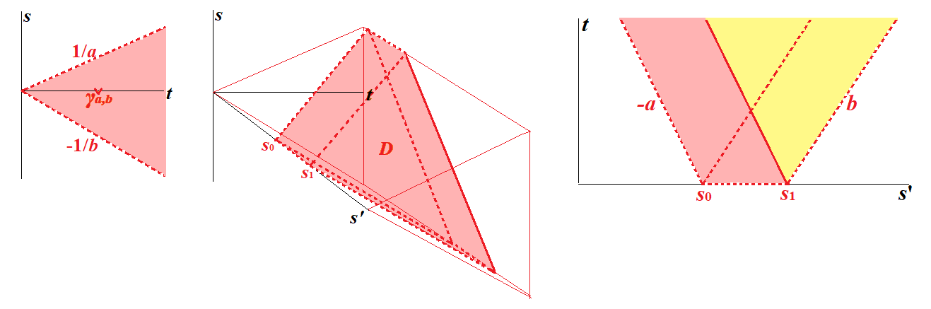
Figure 4. The figure on the left is the open cone $(\gamma_{a,b}^{\vee})^{\circ}$; the one in the middle is the subset $D$ forgetting the $t^{\prime}$ coordinate; the one on the right is the projection $p(D)$ forgetting the $t^{\prime}$ coordinate, where the fibers in the yellow region are half closed half open intervals and the fibers in the red region are open intervals.

Proof of Theorem 5.3.

The movie of a subset $\Lambda\subset T^{*}(M\times\mathbb{R})$ under the Hamiltonian isotopy $\varphi_{\widehat{H}}^{s}\,(s\in I)$ is

$$\Lambda_{H}=\{(x,t,s,\xi,\tau,\sigma)|(x,t,\xi,\tau)=\varphi_{\widehat{H}}^{s}(x_{0},t_{0},\xi_{0},\tau_{0}),\,\nu=-\tau H_{s}\circ\widehat{\varphi}_{H}^{s}(x,t,\xi/\tau)\}.$$

Therefore it follows immediately that in an interval $[s_{i-1},s_{i}]$, one can choose $r>0$ small such that

$$SS(\mathscr{H})\cap T^{*}(M\times\mathbb{R}\times(s_{i-1}-r,s_{i}+r))\subset T^{*}M\times\left((\mathbb{R}\times I)\times\gamma_{a_{i},b_{i}}\right),$$

where $a_{i}=\max_{s\in(s_{i-1}-r,s_{i}+r)}{H_{s}},\,b_{i}=-\min_{s\in(s_{i-1}-r,s_{i}+r)}{H_{u}}$. This will enable us to apply Lemma 5.4 later.

Write $\pi=\pi_{M\times\mathbb{R}}:M\times\mathbb{R}^{2}\rightarrow M\times\mathbb{R}$. To connect $\mathscr{H}|_{M\times\mathbb{R}\times\{s_{i-1}\}}$ and $\mathscr{H}|_{M\times\mathbb{R}\times\{s_{i}\}}$, we consider the following exact triangles

$$\begin{split}\pi_{*}(\mathscr{H}|_{M\times\mathbb{R}\times[s_{i-1},s_{i})})&\rightarrow\pi_{*}(\mathscr{H}|_{M\times\mathbb{R}\times[s_{i-1},s_{i}]})\rightarrow\pi_{*}(\mathscr{H}|_{M\times\mathbb{R}\times\{s_{i}\}})\xrightarrow{+1},\\ \pi_{*}(\mathscr{H}|_{M\times\mathbb{R}\times(s_{i-1},s_{i}]})&\rightarrow\pi_{*}(\mathscr{H}|_{M\times\mathbb{R}\times[s_{i-1},s_{i}]})\rightarrow\pi_{*}(\mathscr{H}|_{M\times\mathbb{R}\times\{s_{i-1}\}})\xrightarrow{+1}.\end{split}$$

Consider the commutative diagram given by natural morphisms under translation

By Lemma 5.4, when $c=a_{i}(s_{i}-s_{i-1})+\epsilon$, the left vertical arrow is zero. Hence by the commutative diagram

the composition

$$\pi_{*}(\mathscr{H}|_{M\times\mathbb{R}\times\{s_{i}\}})\rightarrow T_{c,*}\pi_{*}(\mathscr{H}|_{M\times\mathbb{R}\times\{s_{i}\}})\rightarrow T_{c,*}\pi_{*}(\mathscr{H}|_{M\times\mathbb{R}\times[s_{i-1},s_{i})})[1]$$

is zero. In other words, there exists a morphism

$$\pi_{*}(\mathscr{H}|_{M\times\mathbb{R}\times\{s_{i}\}})\xrightarrow{\phi}T_{c,*}\pi_{*}(\mathscr{H}|_{M\times\mathbb{R}\times[s_{i-1},s_{i}]})$$

that makes the diagram commute. This shows that

$$\pi_{*}(\mathscr{H}|_{M\times\mathbb{R}\times\{s_{i}\}}),\,\,\,\pi_{*}(\mathscr{H}|_{M\times\mathbb{R}\times[s_{i-1},s_{i}]})$$

are $(0,a_{i}(s_{i}-s_{i-1})+\epsilon)$-interleaved. Similarly,

$$\pi_{*}(\mathscr{H}|_{M\times\mathbb{R}\times\{s_{i-1}\}}),\,\,\,\pi_{*}(\mathscr{H}|_{M\times\mathbb{R}\times[s_{i-1},s_{i}]})$$

are $(b_{i}(s_{i}-s_{i-1})+\epsilon,0)$-interleaved. By Lemma 5.2, this means $\pi_{*}(\mathscr{H}|_{M\times\mathbb{R}\times\{s_{i-1}\}})$ and $\pi_{*}(\mathscr{H}|_{M\times\mathbb{R}\times\{s_{i}\}})$ will be $(b_{i}(s_{i}-s_{i-1})+\epsilon,a_{i}(s_{i}-s_{i-1})+\epsilon)$-interleaved.

Now we choose a division of $[0,1]$, then by Lemma 5.2, we know $\pi_{*}(\mathscr{H}|_{M\times\mathbb{R}\times\{0\}})$ and $\pi_{*}(\mathscr{H}|_{M\times\mathbb{R}\times\{1\}})$ are $(a,b)$-interleaved where

$$a=\sum_{i=1}^{N}a_{i}(s_{i}-s_{i-1})+N\epsilon,\,\,\,b=\sum_{i=1}^{N}b_{i}(s_{i}-s_{i-1})+N\epsilon$$

are the Riemann sums. Therefore by letting $\epsilon\ll 1/N$ we know that

$$d(\mathscr{H},\Phi_{H}^{1}(\mathscr{H}))\leq\inf_{0=s_{0}<...<s_{N}=1}\left\{\sum_{i=1}^{N}\Big{(}\max_{(s_{i-1}-r,s_{i}+r)}{H_{s}}-\min_{(s_{i-1}-r,s_{i}+r)}{H_{s}}\Big{)}(s_{i}-s_{i-1})\right\},$$

so the result follows. ∎

Using this machinery, we now study our sheaf $\mathscr{H}om(\mathscr{F}_{q},\mathscr{G}_{r})$ for $\mathscr{F,G}\in Sh^{b}(M\times\mathbb{R})$. As we have seen in previous sections, the last $\mathbb{R}$ component encodes the length of all Reeb chords on $\Lambda$. Hence in order to get information on how the Reeb chords change under Hamiltonian isotopies, we project the sheaf to the last component $\mathbb{R}$ via $u:M\times\mathbb{R}^{2}\rightarrow\mathbb{R},\,\,(x,t,u)\mapsto u$ and estimate the persistence structure on

$$u_{*}\mathscr{H}om(\mathscr{F}_{q},\mathscr{G}_{r}).$$

By Lemma 4.1, this is a constructible sheaf in $Sh^{b}_{\nu<0}(\mathbb{R})$. Here is our main result in this section.

Definition 5.4 (Definition 1.4).

Let $q:M\times\mathbb{R}^{2}\rightarrow M\times\mathbb{R}$ be $q(x,t,u)=(x,t)$ and $r:M\times\mathbb{R}^{2}\rightarrow M\times\mathbb{R}$ be $r(x,t,u)=(x,t-u)$. For sheaves $\mathscr{F,G}\in Sh^{b}(M\times\mathbb{R})$, let

$$\mathscr{H}om_{(-\infty,+\infty)}(\mathscr{F,G})=u_{*}\mathscr{H}om(\mathscr{F}_{q},\mathscr{G}_{r}).$$

Theorem 5.5 (Theorem 1.9).

Let $\Lambda\subset T^{*,\infty}_{\tau>0}(M\times\mathbb{R})$ be a compact Legendrian, $H$ be a Hamiltonian on $T^{*,\infty}_{\tau>0}(M\times\mathbb{R})$ and $\Phi_{H}^{s}\,(s\in I)$ be its sheaf quantization. Then for $\mathscr{F,G}\in Sh^{b}_{\Lambda}(M\times\mathbb{R})$ with compact support,

$$d(\mathscr{H}om_{(-\infty,+\infty)}(\mathscr{F,G}),\mathscr{H}om_{(-\infty,+\infty)}(\mathscr{F},\Phi_{H}^{1}(\mathscr{G})))\leq\|H\|_{\text{osc}}.$$

Proof.

First of all we extend $H$ to a compactly supported Hamiltonian on $T^{*,\infty}_{\tau>0}(M\times\mathbb{R}^{2})$. Namely choose a compactly supported cutoff function $\beta_{0}$ on $T^{*,\infty}_{\tau>0}(M\times\mathbb{R})$ such that

$$\beta_{0}|_{\bigcup_{s\in I}\varphi_{H}^{s}(\Lambda)}\equiv 1.$$

Let $H_{0}=\beta_{0}H$ be a compactly supported Hamiltonian on $T^{*,\infty}_{\tau>0}(M\times\mathbb{R})$. Then we can define $\widehat{H}_{0}(x,t,u,\xi,\tau,\nu)=\beta_{0}(x,t-u,\xi,\tau)H(x,t-u,\xi,\tau)$. Since $\mathrm{supp}(\mathscr{F}),\mathrm{supp}(\mathscr{G})$ are compact, we may assume that there exists $c>0$,

$$q^{-1}(\mathrm{supp}(\mathscr{F}))\cap r^{-1}\Big{(}\bigcup_{s\in I}\pi\big{(}\varphi_{H}^{s}(\pi^{-1}(\mathrm{supp}(\mathscr{G})))\big{)}\Big{)}\subset M\times[-c,c]^{2},$$

where $\pi:T^{*,\infty}(M\times\mathbb{R})\rightarrow M\times\mathbb{R}$ is the projection. Choose a compactly supported cutoff function $\widehat{\beta}_{1}$ on $T^{*,\infty}_{\tau>0}(M\times\mathbb{R}^{2})$ such that

$$\widehat{\beta}_{1}|_{M\times[-c,c]^{2}}\equiv 1.$$

Then let $\widehat{H}(x,t,u,\xi,\tau,\nu)=\widehat{\beta}_{1}(x,t,u)\widehat{H}_{0}(x,t,u,\xi,\tau,\nu)$. One can see that

$$\mathscr{H}om(\mathscr{F}_{q},(\Phi_{H}^{s}\mathscr{G})_{r})=\mathscr{H}om(\mathscr{F}_{q},\Phi_{\widehat{H}_{0}}^{s}(\mathscr{G}_{r}))=\mathscr{H}om(\mathscr{F}_{q},\Phi_{\widehat{H}}^{s}(\mathscr{G}_{r})).$$

We try to show that

$$d(u_{*}\mathscr{H}om(\mathscr{F}_{q},\mathscr{G}_{r}),u_{*}\mathscr{H}om(\mathscr{F}_{q},(\Phi_{H}^{1}\mathscr{G})_{r})\leq d(\mathscr{G}_{r},\Phi_{H}^{1}(\mathscr{G}_{r})).$$

Namely, if $\mathscr{G}_{r},\mathscr{G}^{\prime}_{r}$ are $(\epsilon,\epsilon^{\prime})$-interleaved, then $u_{*}\mathscr{H}om(\mathscr{F}_{q},\mathscr{G}_{r}),\,u_{*}\mathscr{H}om(\mathscr{F}_{q},\mathscr{G}^{\prime}_{r})$ will also be $(\epsilon,\epsilon^{\prime})$-interleaved. Let $T_{c}(x,t,u)=(x,t+c,u)$ and $U_{c}(x,t,u)=(x,t,u-c)$. Then since $r\circ T_{c}=r\circ U_{c}$ and $q=q\circ U_{c}$,

$$\mathscr{H}om(\mathscr{F}_{q},T_{c,*}\mathscr{G}_{r})=\mathscr{H}om(U_{c,*}\mathscr{F}_{q},U_{c,*}\mathscr{G}_{r})=U_{c,*}\mathscr{H}om(\mathscr{F}_{q},\mathscr{G}_{r}).$$

For any morphism $\mathscr{G}_{r}\rightarrow T_{c,*}\mathscr{G}^{\prime}_{r}$ there is a canonical morphism

$$\mathscr{H}om(\mathscr{F}_{q},\mathscr{G}_{r})\rightarrow\mathscr{H}om(\mathscr{F}_{q},T_{c,*}\mathscr{G}^{\prime}_{r}).$$

Therefore there is always a canonical morphism

$$\mathscr{H}om(\mathscr{F}_{q},\mathscr{G}_{r})\rightarrow U_{c,*}\mathscr{H}om(\mathscr{F}_{q},\mathscr{G}^{\prime}_{r}).$$

By abuse of notations, we also write $U_{c}:\mathbb{R}\rightarrow\mathbb{R},\,u\mapsto u-c$. Note that $u\circ U_{c}=U_{c}$, so one will have a canonical morphism

$$u_{*}\mathscr{H}om(\mathscr{F}_{q},\mathscr{G}_{r})\rightarrow U_{c,*}u_{*}\mathscr{H}om(\mathscr{F}_{q},\mathscr{G}^{\prime}_{r}).$$

This shows that if $\mathscr{G}_{r},\mathscr{G}^{\prime}_{r}$ are $(\epsilon,\epsilon^{\prime})$-interleaved, then $u_{*}\mathscr{H}om(\mathscr{F}_{q},\mathscr{G}_{r}),\,u_{*}\mathscr{H}om(\mathscr{F}_{q},\mathscr{G}^{\prime}_{r})$ will also be $(\epsilon,\epsilon^{\prime})$-interleaved, and hence completes the proof. ∎

Here are two examples about $\mathscr{H}om_{(-\infty,+\infty)}(\Bbbk_{(x_{0},t_{0})},\mathscr{F})$ for the skyscraper sheaf $\Bbbk_{(x_{0},t_{0})}$ and $\mathscr{F}\in Sh^{b}_{\Lambda}(\mathbb{R}^{2})$. We will see that $\mathscr{H}om_{(-\infty,+\infty)}(\Bbbk_{(x_{0},t_{0})},\mathscr{F})$ detects Reeb chords between $\Lambda$ and the cotangent fiber $T^{*,\infty}_{(x_{0},t_{0})}(M\times\mathbb{R})$.

Note that although $\Bbbk_{(x_{0},t_{0})}\notin Sh_{\tau>0}^{b}(\mathbb{R}^{2})$, one can still apply the same argument in Proposition 3.5 and Lemma 4.1, and find that $\mathscr{H}om_{(-\infty,+\infty)}(\Bbbk_{(x_{0},t_{0})},\mathscr{F})\in Sh_{\nu<0}^{b}(\mathbb{R})$.

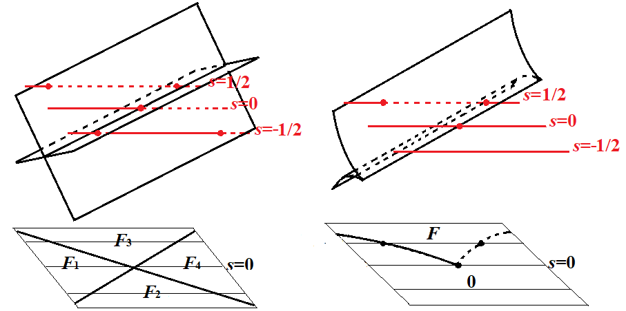
Figure 5. Birth-death of Reeb chords (on the right) and swapping of Reeb chords (on the left). On the top, the black Legendrians are $(\Lambda_{s})_{r}$ while the red curves are $(T^{*,\infty}_{(0,1)}\mathbb{R}^{2})_{q}$. The $u$-axis is horizontal, the $t$-axis is vertical, while the $s$-axis is pointing into the blackboard.

Example 5.3.

The first example is about birth-death of Reeb chords (Figure 5 right). We consider a family of Legendrians $\Lambda_{s}=\{(x,\pm 3(x+s)^{1/2}/2,(x+s)^{3/2})|x+s\geq 0\}\subset J^{1}(\mathbb{R})$ whose front projections are standard cusps $\{(x,t)|t^{2}=(x+s)^{3}\}$. Consider Reeb chords from $\Lambda_{s}$ to the fiber $T^{*,\infty}_{(0,1)}\mathbb{R}^{2}$. At $s=0$, a pair of Reeb chords are created.

For $F\in Mod(\Bbbk)$, consider the sheaf

$$\mathscr{F}_{s}=F_{\{(x,t)|0\leq t<(x+s)^{3/2}\text{ or }(x+s)^{3/2}\leq t<0\}}.$$

Then consider $u_{*}\mathscr{H}om((\Bbbk_{(0,1)})_{q},\mathscr{F}_{r})$. One can see that

$$u_{*}\mathscr{H}om((\Bbbk_{(0,1)})_{q},(\mathscr{F}_{s})_{r})_{u=c}=\Gamma(\mathbb{R},\mathscr{H}om(\Bbbk_{(0,1)},T_{c,*}\mathscr{F}_{s}))=\mathscr{F}_{s}|_{(x,t)=(0,1-c)}.$$

Therefore when $s\leq 0$, we have $\mathscr{H}om_{(-\infty,+\infty)}(\Bbbk_{(0,1)},\mathscr{F}_{s})=0$. When $s>0$,

$$\mathscr{H}om_{(-\infty,+\infty)}(\Bbbk_{(0,1)},\mathscr{F}_{s})=F_{(1-s^{3/2},1+s^{3/2}]}.$$

In other words, the birth of Reeb chords creates a new bar.

When the Hamiltonian isotopy swaps the length of two Reeb chords, the behaviour of the sheaf $\mathscr{H}om_{(-\infty,+\infty)}(-,-)$ under the isotopy may be more complicated. However, there are still very specific cases where the behaviour is relatively clear.

Example 5.4.

The second example is a specific case of swapping of Reeb chords (Figure 5 left). We consider a family of Legendrians $\Lambda_{s}=\{(x,\pm 1,\pm(x+s))|x\in\mathbb{R}\}\subset J^{1}(\mathbb{R})$ whose front projections are standard crossings $\{(x,t)|t=\pm(x+s)\}$. Consider Reeb chords from $\Lambda_{s}$ to the fiber $T^{*,\infty}_{(0,1)}\mathbb{R}^{2}$. At $s=0$, a pair of Reeb chords are swapped.

For $F_{1},F_{2},F_{3},F_{4}\in Mod(\Bbbk)$, suppose for $\mathscr{F}=\mathscr{F}_{0}$,

$$\begin{split}\mathscr{F}|_{\{(x,y)|t\geq|x|\}}=F_{1}|_{\{(x,y)|t\geq|x|\}},\,&\,\mathscr{F}|_{\{(x,y)|t<-|x|\}}=F_{4}|_{\{(x,y)|t<-|x|\}}\\ \mathscr{F}|_{\{(x,y)|x<0,-t<x\leq t\}}=F_{2}|_{\{(x,y)|x<0,-t<x\leq t\}},\,&\,\mathscr{F}|_{\{(x,y)|x>0,-t<x\leq t\}}=F_{1}|_{\{(x,y)|x>0,-t<x\leq t\}}.\end{split}$$

The sheaf $\mathscr{F}$ is characterized by the diagram (see Example 3.5 or [STZ, Section 3.3])

where $\mathrm{Tot}\,(F_{1}\rightarrow F_{2}\oplus F_{3}\rightarrow F_{4})\simeq 0$ (see [STZ, Section 3.3 & 3.4]). Then $u_{*}\mathscr{H}om((\Bbbk_{(0,1)})_{q},$ $\mathscr{F}_{r})_{u=c}=\mathscr{F}_{s}|_{(x,t)=(0,1-c)}$. When $s<0$, $\mathscr{H}om_{(-\infty,+\infty)}(\Bbbk_{(0,1)},\mathscr{F}_{s})$ is determined by the diagram

$$F_{1}\longrightarrow F_{2}\longrightarrow F_{4}.$$

When $s>0$, $\mathscr{H}om_{(-\infty,+\infty)}(\Bbbk_{(0,1)},\mathscr{F}_{s})$ is characterized by the diagram

$$F_{1}\longrightarrow F_{3}\longrightarrow F_{4}.$$

Decomposing the sheaf as $\bigoplus_{\alpha\in A}\Bbbk_{(a_{\alpha},b_{\alpha}]}^{r_{\alpha}}[n_{\alpha}]$, we have for $s<0$,

$$\begin{split}\mathscr{H}om_{(-\infty,+\infty)}(\Bbbk_{(0,1)},\mathscr{F}_{s})\simeq&\,V_{(-\infty,+\infty)}\oplus V_{(-\infty,-s]}\oplus V_{(-\infty,s]}\\ &\,\oplus V_{(-s,s]}\oplus V_{(-s,+\infty)}\oplus V_{(s,+\infty)}.\end{split}$$

When $s>0$,

$$\begin{split}\mathscr{H}om_{(-\infty,+\infty)}(\Bbbk_{(0,1)},\mathscr{F}_{s})\simeq&\,U_{(-\infty,+\infty)}\oplus U_{(-\infty,-s]}\oplus U_{(-\infty,s]}\\ &\,\oplus U_{(-s,s]}\oplus U_{(-s,+\infty)}\oplus U_{(s,+\infty)}.\end{split}$$

Using the condition $\mathrm{Tot}\,(F_{1}\rightarrow F_{2}\oplus F_{3}\rightarrow F_{4})\simeq 0$, one can show that

$$\begin{array}[]{c}V_{(-s,s]}\simeq U_{(-s,s]}\simeq 0,\\ V_{(-\infty,-s]}\simeq U_{(-\infty,s]},\,\,V_{(-s,+\infty)}\simeq U_{(s,+\infty)},\\ V_{(-\infty,s]}\simeq U_{(-\infty,-s]},\,\,V_{(s,+\infty)}\simeq U_{(-s,+\infty)},\\ V_{(-\infty,+\infty)}\simeq U_{(-\infty,+\infty)}.\end{array}$$

Hence in this specific case, swapping of Reeb chords swaps starting/ending points of bars (Caution: this may not be true in general).

6. Reeb Chord Estimation

Our goal in this section is to relate the number of Reeb chords with $Hom_{+}(\mathscr{F,F})$ and $\mathscr{H}om_{(-\infty,+\infty)}(\mathscr{F,F})$, and hence finish the proof of Theorem 1.1, 1.2 and 1.3.

6.1. Local Calculation for Microstalks

By Lemma 4.1, we know that certain covectors in the singular support of $\mathscr{H}om(\mathscr{F}_{q},\mathscr{F}_{r})$ correspond to Reeb chords. The microlocal Morse inequality (Proposition 3.7) relates the global section of sheaves to its microstalks. Hence it suffices to determine if the ranks of the microstalks

$$\Gamma_{u\leq u_{i}}(\mathscr{H}om(\mathscr{F}_{q},\mathscr{F}_{r}))_{(x_{i},t_{i},u_{i})}$$

are as expected. This will follow from concrete local calculations. Here is the main result.

Proposition 6.1.

For $\Lambda\subset T^{*,\infty}_{\tau>0}(M\times\mathbb{R})$ a chord generic Legendrian and $\mathscr{F}\in Sh^{b}_{\Lambda}(M\times\mathbb{R})$ a sheaf with perfect microstalk $F$, let $\{(x_{i},0,t_{i},0,u_{i},\nu_{i})\}_{i\in I}$ be the set

$$((-\Lambda_{q})+\Lambda_{r})\cap\{(x,0,t,0,u,\nu)|u>0,\nu<0\}.$$

Suppose $(x_{i},t_{i},u_{i})$ corresponds to a degree $d_{i}$ Reeb chord in Lemma 4.1. Then

$$\Gamma_{u\leq u_{i}}(\mathscr{H}om(\mathscr{F}_{q},\mathscr{F}_{r}))_{(x_{i},t_{i},u_{i})}\simeq Hom(F,F)[-d_{i}].$$

First of all, let’s recall from Section 2 that the degree of a Reeb chord $\gamma\in\mathcal{Q}_{+}(\Lambda)$ is defined as follows. Suppose at $a=(x,\xi,t,\tau)$ and $b=(x,\xi,t+u,\tau)$ ($u>0$),

$$n-\deg(\gamma)=d(a)-d(b)+\mathrm{ind}(D^{2}h_{ab})-1,$$

where $d(b),d(a)$ are Maslov potentials at $b,a$, and $h_{ab}=h_{b}-h_{a}$ for $h_{b},h_{a}$ whose graphs at $b,a$ are $\pi_{\text{front}}(\Lambda)$. By Morse lemma, we assume that in local coordinates

$$h_{b}(x)=u,\,\,\,h_{a}(x)=-\sum_{i\leq k}x_{i}^{2}+\sum_{j\geq k+1}x_{j}^{2}.$$

Next, by microlocal Morse lemma as in Example 3.6 we consider

$$\begin{split}\Gamma_{u\leq u_{i}}(\mathscr{H}om(\mathscr{F}_{q},\mathscr{F}_{r}))_{(x_{i},t_{i},u_{i})}=\mathrm{Cone}&(\Gamma(U_{x_{i},t_{i}}\times(u_{i}-\epsilon,u_{i}+\epsilon),\mathscr{H}om(\mathscr{F}_{q},\mathscr{F}_{r}))\\ &\rightarrow\Gamma(U_{x_{i},t_{i}}\times(u_{i},u_{i}+\epsilon),\mathscr{H}om(\mathscr{F}_{q},\mathscr{F}_{r})))[-1].\end{split}$$

Since $((-\Lambda_{q})+\Lambda_{r})\cap\{(x,0,t,0,u,\nu)|u>0,\nu>0\}=\emptyset$, we know that

$$\Gamma(U_{x_{i},t_{i}}\times(u_{i}-\epsilon,u_{i}+\epsilon),\mathscr{H}om(\mathscr{F}_{q},\mathscr{F}_{r}))\simeq\Gamma(U_{x_{i},t_{i}}\times(u_{i}-\epsilon,u_{i}),\mathscr{H}om(\mathscr{F}_{q},\mathscr{F}_{r})).$$

Hence it suffices to calculate

$$\begin{split}\mathrm{Cone}\big{(}&\Gamma(U_{x_{i},t_{i}}\times(u_{i}-\epsilon,u_{i}),\mathscr{H}om(\mathscr{F}_{q},\mathscr{F}_{r}))\\ &\rightarrow\Gamma(U_{x_{i},t_{i}}\times(u_{i},u_{i}+\epsilon),\mathscr{H}om(\mathscr{F}_{q},\mathscr{F}_{r}))\big{)}[-1].\end{split}$$

Note that $(\Lambda_{q}\cup\Lambda_{r})\cap T^{*,\infty}(U_{x_{i},t_{i}}\times(u_{i}-\epsilon,u_{i}))$ and $(\Lambda_{q}\cup\Lambda_{r})\cap T^{*,\infty}(U_{x_{i},t_{i}}\times(u_{i},u_{i}+\epsilon))$ are movies of Legendrian isotopies. Hence by Guillermou-Kashiwara-Schapira Theorem 3.14, it suffices to compute

$$\begin{split}\mathrm{Cone}\big{(}&\Gamma(U_{x_{i},t_{i}}\times\{u_{i}-\epsilon/2\},\mathscr{H}om(\mathscr{F}_{q},\mathscr{F}_{r})))\\ &\rightarrow\Gamma(U_{x_{i},t_{i}}\times\{u_{i}+\epsilon/2\},\mathscr{H}om(\mathscr{F}_{q},\mathscr{F}_{r}))\big{)}[-1]\end{split}$$

(as long as we can keep track of the restriction map). From now on, we write

$$U^{-}=U_{x_{i},t_{i}}\times\{u_{i}-\epsilon/2\},\,\,\,U^{+}=U_{x_{i},t_{i}}\times\{u_{i}+\epsilon/2\}.$$

Since $(-\Lambda_{q})\cap\Lambda_{r}=\emptyset$, by Proposition 3.5

$$\mathscr{H}om(\mathscr{F}_{q},\mathscr{F}_{r})\simeq D^{\prime}\mathscr{F}_{q}\otimes\mathscr{F}_{r},$$

where $D^{\prime}\mathscr{F}_{q}\in Sh_{-\Lambda_{q}}(M\times\mathbb{R}^{2})$. Now write

$$\begin{split}U^{\pm}\cap\{(x,t)|t>h_{b}(x)\}=U_{q,0},\,&\,U^{\pm}\cap\{(x,t)|t\leq h_{b}(x)\}=U_{q,1},\\ U^{\pm}\cap\{(x,t)|t<h_{a}(x)+u_{i}\pm\epsilon/2\}=U_{r,0}^{\pm},\,&\,U^{\pm}\cap\{(x,t)|t\geq h_{a}(x)+u_{i}\pm\epsilon/2\}=U_{r,1}^{\pm}.\end{split}$$

Without loss of generality by microlocal Morse lemma, as in Example 3.5 or [STZ, Section 3.3] we may assume

$$\begin{split}D^{\prime}\mathscr{F}_{q}|_{U_{q,0}}\simeq Q_{0}|_{U_{q,0}},\,&\,D^{\prime}\mathscr{F}_{q}|_{U_{q,1}}\simeq Q_{1}|_{U_{q,1}},\\ \mathscr{F}_{r}|_{U_{r,0}^{\pm}}\simeq R_{0}|_{U_{r,0}^{\pm}},\,&\,\mathscr{F}_{r}|_{U_{r,1}^{\pm}}\simeq R_{1}|_{U_{r,1}^{\pm}}.\end{split}$$

In addition here we claim that

$$\mathrm{Cone}(Q_{1}\rightarrow Q_{0})\simeq D^{\prime}F[-d(b)],\,\,\mathrm{Cone}(R_{1}\rightarrow R_{0})\simeq F[d(a)+1].$$

Lemma 6.2.

Let $\mathscr{F}\in Sh_{T^{*,\infty}_{\mathbb{R}^{n}\times\mathbb{R}_{>0},-}\mathbb{R}^{n+1}}^{b}(\mathbb{R}^{n+1})$ and $\varphi(x,t)=t$. Then

$$R\Gamma_{\varphi\leq 0}(D^{\prime}\mathscr{F})_{(0,...,0)}=D^{\prime}R\Gamma_{\varphi\geq 0}(\mathscr{F})_{(0,...,0)}[-1].$$

Proof.

We assume that $\mathscr{F}|_{\mathbb{R}^{n}\times[0,+\infty)}=F_{1}|_{\mathbb{R}^{n}\times[0,+\infty)}$ and $\mathscr{F}|_{\mathbb{R}^{n}\times(-\infty,0)}=F_{0}|_{\mathbb{R}^{n}\times(-\infty,0)}$. Then we have an exact triangle

$$\Gamma_{\varphi\geq 0}(\mathscr{F})_{(0,0)}\rightarrow F_{1}\rightarrow F_{0}\xrightarrow{+1}.$$

Therefore by taking the dual we have

$$D^{\prime}F_{0}\rightarrow D^{\prime}F_{1}\rightarrow D^{\prime}\Gamma_{\varphi\geq 0}(\mathscr{F})_{(0,0)}\xrightarrow{+1}.$$

However, we claim $D^{\prime}\mathscr{F}|_{\mathbb{R}^{n}\times(0,+\infty)}=D^{\prime}F_{1}|_{\mathbb{R}^{n}\times(0,+\infty)}$ and $D^{\prime}\mathscr{F}|_{\mathbb{R}^{n}\times(-\infty,0]}=D^{\prime}F_{0}|_{\mathbb{R}^{n}\times(-\infty,0]}$. We will only check the stalk at $\mathbb{R}^{n}\times\{0\}$ (other stalks can be computed easily). In fact

$$D^{\prime}\mathscr{F}_{(0,0)}=\Gamma(\{(0,...,0)\},\mathscr{H}om(\mathscr{F},\Bbbk))\simeq\Gamma(\mathbb{R}^{n+1},\mathscr{H}om(\mathscr{F},\Bbbk)),$$

and the latter consists of morphisms $\phi_{1}:F_{1}\rightarrow\Bbbk,\phi_{0}:F_{0}\rightarrow\Bbbk$ such that the following diagram commutes:

Such pairs $(\phi_{1},\phi_{0})$ corresponds bijectively to $\phi_{0}:F_{0}\rightarrow\Bbbk$ ($\phi_{1}$ will just be the composition of $\phi_{0}$ and the restriction map $F_{1}\rightarrow F_{0}$), so

$$Hom(\mathscr{F},\Bbbk)\simeq Hom(F_{0},\Bbbk)=D^{\prime}F_{0}.$$

Therefore we know that

$$\Gamma_{\varphi\leq 0}(D^{\prime}\mathscr{F})_{(0,...,0)}=\mathrm{Cone}(D^{\prime}F_{0}\rightarrow D^{\prime}F_{1})[-1]\simeq D^{\prime}\Gamma_{\varphi\geq 0}(\mathscr{F})_{(0,...,0)}[-1].$$

This proves the assertion. ∎

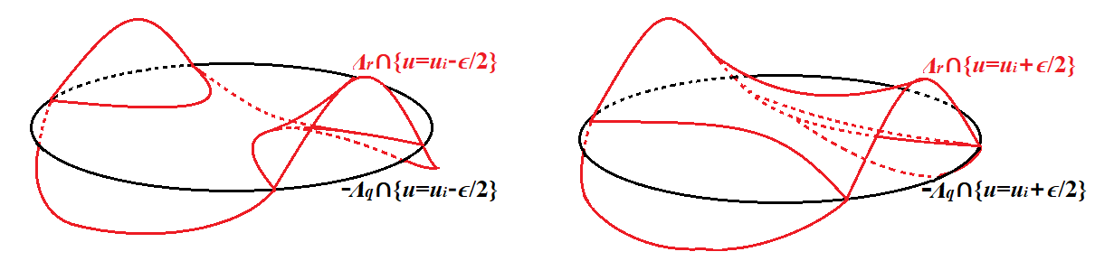
Figure 6. When $n=2$ and $k=1$, the open subsets $U^{-}$ (on the left) and $U^{+}$ (on the right).

Suppose first $0<k<n$. Now we compute $R\Gamma(U_{(x_{i},t_{i})}\times\{u_{i}\pm\epsilon/2\},R\mathscr{H}om(\mathscr{F}_{q},\mathscr{F}_{r}))$ separately. At $u=u_{i}-\epsilon/2$, we know that

$$\begin{split}U_{q,1}\cap U_{r,0}^{-}\cong D^{k}\times D^{n-k}\times(0,1],&\,U_{q,0}\cap U_{r,1}^{-}\cong D^{k}\times D^{n-k}\times[0,1),\\ U_{q,1}\cap U_{r,1}^{-}\cong D^{k}\times D^{n-k}\times[0,1],\,U_{q,0}&\cap U_{r,0}^{-}\cong D^{k}\times(S^{n-k-1}\times(0,1))\times(0,1).\end{split}$$

At $u=u_{i}+\epsilon/2$, we know that

$$\begin{split}U_{q,1}\cap U_{r,0}^{+}\cong D^{k}\times D^{n-k}\times(0,1],\,U_{q,0}\,\cap&\,U_{r,1}^{+}\cong D^{k}\times D^{n-k}\times[0,1),\\ U_{q,1}\cap U_{r,1}^{+}\cong(S^{k-1}\times[0,1))\times D^{n-k}\times[0,1],&\,U_{q,0}\cap U_{r,0}^{+}\cong D^{k}\times D^{n-k}\times(0,1),\end{split}$$

and the boundary regions around $\overline{U_{q,0}\cap U_{r,0}^{-}}$ are (Figure 7)

$$\begin{split}U_{q,1}\cap U_{r,0}^{-}\cap\overline{U_{q,0}\cap U_{r,0}^{-}}=D_{-}^{k}\times D^{n-k},\\ U_{q,0}\cap U_{r,1}^{-}\cap\overline{U_{q,0}\cap U_{r,0}^{-}}=D_{+}^{k}\times D^{n-k},\\ U_{q,1}\cap U_{r,1}^{-}\cap\overline{U_{q,0}\cap U_{r,0}^{-}}=S^{k-1}\times D^{n-k},\end{split}$$

where $D_{-}^{k}\subset S^{k}$ is the lower hemisphere and $D_{+}^{k}\subset S^{k}$ is the upper hemisphere.

Figure 7. When $n=2$ and $k=1$, the stratification on $\overline{U_{q,0}\cap U_{r,0}^{+}}\subset U^{+}$.

Proof of Proposition 6.1.

Suppose first that $0<k<n$. At $u=u_{i}-\epsilon/2$, since $(-\Lambda_{q})\cap\Lambda_{r}\cap\nu^{*,\infty}_{U_{q,1}\cap U_{r,1}^{-},+}(M\times\mathbb{R})=\emptyset$ (recall $\nu^{*,\infty}_{U_{q,1}\cap U_{r,1}^{-},+}(M\times\mathbb{R})$ is the outward conormal), we know by microlocal Morse lemma that

$$\Gamma(U^{-},D^{\prime}\mathscr{F}_{q}\otimes\mathscr{F}_{r})=\Gamma(U_{q,1}\cap U_{r,1}^{-},D^{\prime}\mathscr{F}_{q}\otimes\mathscr{F}_{r})\simeq Q_{1}\otimes R_{1}.$$

At $u=u_{i}+\epsilon/2$, since $(-\Lambda_{q})\cap\Lambda_{r}\cap\nu^{*,\infty}_{U_{q,0}\cap U_{r,0}^{+},+}(M\times\mathbb{R})=\emptyset$, we also know that (see Figure 7)

$$\Gamma(U^{+},D^{\prime}\mathscr{F}_{q}\otimes\mathscr{F}_{r})=\Gamma(\overline{U_{q,0}\cap U_{r,0}^{+}},D^{\prime}\mathscr{F}_{q}\otimes\mathscr{F}_{r}).$$

Here $\overline{U_{q,0}\cap U_{r,0}^{+}}=\overline{D}^{k+1}\times D^{n-k}$ with a statification $D^{k+1}\times D^{n-k},D_{\pm}^{k}\times D^{n-k}$ and $S^{k-1}\times D^{n-k}$. In addition

$$\begin{array}[]{c}D^{\prime}\mathscr{F}_{q}\otimes\mathscr{F}_{r}|_{D^{k+1}\times D^{n-k}}=Q_{0}\otimes R_{0},\\ D^{\prime}\mathscr{F}_{q}\otimes\mathscr{F}_{r}|_{D_{+}^{k}\times D^{n-k}}=Q_{0}\otimes R_{1},\,\,D^{\prime}\mathscr{F}_{q}\otimes\mathscr{F}_{r}|_{D_{-}^{k}\times D^{n-k}}=Q_{1}\otimes R_{1},\\ D^{\prime}\mathscr{F}_{q}\otimes\mathscr{F}_{r}|_{S^{k-1}\times D^{n-k}}=Q_{1}\otimes R_{1}.\end{array}$$

It suffices for us to do calculations on $\overline{D}^{k+1}$, so from now on we will drop all the $D^{n-k}$ terms. In order to calculate the (derived) global sections using Čech cohomology, we need to consider a refinement of the current stratification on $\overline{U_{q,0}\cap U_{r,0}^{+}}$, whose stars give a good cover (meaning that any finite intersection is contractible) of the region. We consider the stratification of $S^{k-1}$ by $\partial\Delta^{k}$, whose stars are

$$\mathrm{St}\Delta_{[i_{1}i_{2}...i_{v}]}=\bigcup_{\{i_{1},i_{2},...,i_{v}\}\subset\{i^{\prime}_{1},i^{\prime}_{2},...,i^{\prime}_{u}\}\subset\{0,1,...,k+1\}}\Delta_{[i^{\prime}_{1}i^{\prime}_{2}...i^{\prime}_{u}]}=\bigcap_{1\leq j\leq v}\mathrm{St}\Delta_{[i_{j}]}.$$

Consider the stars which give a good cover (Figure 8 left). Therefore the (derived) global section is (Figure 8 right)

$$\begin{split}\Gamma\big{(}\overline{U_{q,0}\cap U_{r,0}^{+}},D^{\prime}&\mathscr{F}_{q}\otimes\mathscr{F}_{r}\big{)}\\ \simeq\mathrm{Colim}\big{(}&(Q_{1}\otimes R_{1})^{\oplus k+1}\rightarrow(Q_{1}\otimes R_{1})^{\oplus(k+1)k/2}\rightarrow...\\ &\rightarrow(Q_{1}\otimes R_{1})^{\oplus k+1}\rightarrow(Q_{0}\otimes R_{1})\oplus(Q_{1}\otimes R_{0})\rightarrow(Q_{0}\otimes R_{0})\big{)}.\end{split}$$

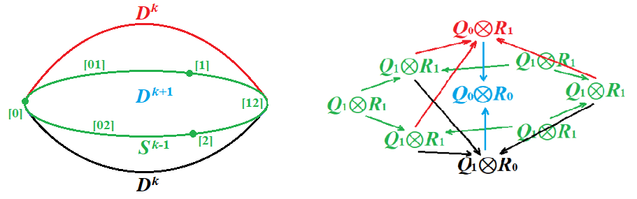
Figure 8. The stratification in the case $k=2$ (left), and the restriction maps pointing from lower dimensional strata to higher dimensional strata (right). These are restriction maps because given the triangulation, the stars of lower dimensional ones contain stars of higher dimensional ones. The green indices on the left are labels of the simplices $\partial\Delta^{k}$.

Before starting to compute the microstalk, we need to keep track of the restriction functor

$$\begin{split}Q_{1}\otimes R_{1}\rightarrow\mathrm{Colim}\big{(}&(Q_{1}\otimes R_{1})^{\oplus k+1}\rightarrow(Q_{1}\otimes R_{1})^{\oplus(k+1)k/2}\rightarrow...\\ &\rightarrow(Q_{1}\otimes R_{1})^{\oplus k+1}\rightarrow(Q_{0}\otimes R_{1})\oplus(Q_{1}\otimes R_{0})\rightarrow(Q_{0}\otimes R_{0})\big{)}.\end{split}$$

Note that in $U=U_{(x_{i},t_{i})}\times(u_{i}-\epsilon,u_{i}+\epsilon)$, the $Q_{1}\otimes R_{1}$ term is supported on $V\simeq D^{k}\times D^{n-k}\times[0,1]\times(0,1]$, where the restriction map is the one induced by

$$C^{*}(D^{k}\times D^{n-k}\times[0,1]\times(0,1];\mathbb{K})\rightarrow C^{*}((S^{k-1}\times[0,1))\times D^{n-k}\times[0,1];\mathbb{K}),$$

which is homotopic to the restriction map $C^{*}(\Delta^{k};\mathbb{K})\rightarrow C^{*}(\partial\Delta^{k};\mathbb{K})$, where $\mathbb{K}=Q_{1}\otimes R_{1}$. Hence the restriction map is just the diagonal map

$$\begin{array}[]{cccc}\delta:&Q_{1}\otimes R_{1}&\rightarrow&(Q_{1}\otimes R_{1})^{\oplus k+1},\\ &x&\mapsto&(x,x,...,x).\end{array}$$

Since the cone of the restriction map is

$$\mathrm{Cone}\big{(}C^{*}(\Delta^{k};\mathbb{K})\rightarrow C^{*}(\partial\Delta^{k};\mathbb{K})\big{)}\simeq C^{*}(\Delta^{k},\partial\Delta^{k};\mathbb{K})\simeq\Bbbk[-k],$$

we are able to calculate the microstalk:

$$\begin{split}\Gamma_{u\leq u_{i}}(D^{\prime}\mathscr{F}_{q}\otimes&\mathscr{F}_{r})_{(x_{i},t_{i},u_{i})}\\ \simeq\mathrm{Cone}\big{(}&(Q_{1}\otimes R_{1})\rightarrow\mathrm{Colim}\big{(}(Q_{1}\otimes R_{1})^{\oplus k+1}\rightarrow...\\ &\rightarrow(Q_{1}\otimes R_{1})^{\oplus k+1}\rightarrow(Q_{0}\otimes R_{1})\oplus(Q_{1}\otimes R_{0})\rightarrow(Q_{0}\otimes R_{0})\big{)}\big{)}[-1]\\ \simeq\hskip 4.0pt\mathrm{Tot}\hskip 2.0pt\big{(}&(Q_{1}\otimes R_{1})\rightarrow(Q_{1}\otimes R_{1})^{\oplus k+1}\rightarrow...\\ &\rightarrow(Q_{1}\otimes R_{1})^{\oplus k+1}\rightarrow(Q_{0}\otimes R_{1})\oplus(Q_{1}\otimes R_{0})\rightarrow(Q_{0}\otimes R_{0})\big{)}\\ \simeq\hskip 4.0pt\mathrm{Tot}\hskip 2.0pt\big{(}&0\rightarrow 0\rightarrow...\rightarrow(Q_{1}\otimes R_{1})\rightarrow\\ &\rightarrow(Q_{0}\otimes R_{1})\oplus(Q_{1}\otimes R_{0})\rightarrow(Q_{0}\otimes R_{0})\big{)}\\ \simeq\hskip 4.0pt\mathrm{Tot}\hskip 2.0pt\big{(}&(Q_{1}\otimes R_{1})\rightarrow(Q_{0}\otimes R_{1})\oplus(Q_{1}\otimes R_{0})\rightarrow(Q_{0}\otimes R_{0})\big{)}[-k].\end{split}$$

By Kunneth’s formula, we can conclude that

$$\begin{split}\mathrm{Tot}\,\big{(}&(Q_{1}\otimes R_{1})\rightarrow(Q_{0}\otimes R_{1})\oplus(Q_{1}\otimes R_{0})\rightarrow(Q_{0}\otimes R_{0})\big{)}[-k]\\ &\simeq\mathrm{Tot}\big{(}Q_{1}\rightarrow Q_{0}\big{)}\otimes\mathrm{Tot}\big{(}R_{1}\rightarrow R_{0}\big{)}[-k]\\ &\simeq\left(D^{\prime}F[-d(b)-1]\otimes F[d(a)]\right)[-k]=D^{\prime}F\otimes F[d_{i}].\end{split}$$

Finally the only case left is the case when $k=0$ or $n$. The strategy is the same. When $k=n$, the sections at $u=u_{i}-\epsilon/2$ are

$$\Gamma(U^{-},D^{\prime}\mathscr{F}_{q}\otimes\mathscr{F}_{r})=\Gamma(\overline{U_{q,1}\cap U_{r,1}^{-}},D^{\prime}\mathscr{F}_{q}\otimes\mathscr{F}_{r})\simeq Q_{1}\otimes R_{1}.$$

The sections at $u=u_{i}+\epsilon/2$ are

$$\begin{split}\Gamma(U^{+},D^{\prime}\mathscr{F}_{q}\otimes\mathscr{F}_{r})&=\Gamma(\overline{U_{q,0}\cap U_{r,0}^{+}},D^{\prime}\mathscr{F}_{q}\otimes\mathscr{F}_{r})\\ \simeq\mathrm{Colim}\big{(}&(Q_{1}\otimes R_{1})^{\oplus n+1}\rightarrow(Q_{1}\otimes R_{1})^{\oplus(n+1)n/2}\rightarrow...\\ &\rightarrow(Q_{1}\otimes R_{1})^{\oplus n+1}\rightarrow(Q_{0}\otimes R_{1})\oplus(Q_{1}\otimes R_{0})\rightarrow(Q_{0}\otimes R_{0})\big{)}[-1].\end{split}$$

Hence by the same argument using Kunneth’s formula, the microstalk is

$$\begin{split}\Gamma_{u\leq u_{i}}(D^{\prime}&\mathscr{F}_{q}\otimes\mathscr{F}_{r})_{(x_{i},t_{i},u_{i})}\\ \simeq&\hskip 2.0pt\mathrm{Tot}\,\big{(}(Q_{1}\otimes R_{1})\rightarrow(Q_{1}\otimes R_{1})^{\oplus n+1}\rightarrow...\\ &\rightarrow(Q_{1}\otimes R_{1})^{\oplus n+1}\rightarrow(Q_{0}\otimes R_{1})\oplus(Q_{1}\otimes R_{0})\rightarrow(Q_{0}\otimes R_{0})\big{)}\\ \simeq&\hskip 2.0pt\mathrm{Tot}\,\big{(}(Q_{1}\otimes R_{1})\rightarrow(Q_{0}\otimes R_{1})\oplus(Q_{1}\otimes R_{0})\rightarrow(Q_{0}\otimes R_{0})\big{)}[-n]\\ \simeq&\hskip 2.0pt\mathrm{Tot}\big{(}Q_{1}\rightarrow Q_{0}\big{)}\otimes\mathrm{Tot}\big{(}R_{1}\rightarrow R_{0}\big{)}[-n]\\ \simeq&\left(D^{\prime}F[-d(b)-1]\otimes F[d(a)]\right)[-n]=D^{\prime}F\otimes F[d_{i}].\end{split}$$

When $k=0$, the sections at $u=u_{i}-\epsilon/2$ are

$$\Gamma(U^{-},D^{\prime}\mathscr{F}_{q}\otimes\mathscr{F}_{r})=\Gamma(\overline{U_{q,1}\cap U_{r,1}^{-}},D^{\prime}\mathscr{F}_{q}\otimes\mathscr{F}_{r})\simeq Q_{1}\otimes R_{1}.$$

The sections at $u=u_{i}+\epsilon/2$ are

$$\begin{split}\Gamma(U^{+},D^{\prime}\mathscr{F}_{q}\otimes\mathscr{F}_{r})&=\Gamma(\overline{U_{q,0}\cap U_{r,0}^{+}},D^{\prime}\mathscr{F}_{q}\otimes\mathscr{F}_{r})\\ &\simeq\mathrm{Colim}\left((Q_{1}\otimes R_{0})\oplus(Q_{0}\otimes R_{1})\rightarrow(Q_{0}\rightarrow R_{0})\right).\end{split}$$

Therefore the microstalk is

$$\begin{split}\Gamma_{u\leq u_{i}}(&D^{\prime}\mathscr{F}_{q}\otimes\mathscr{F}_{r})_{(x_{i},t_{i},u_{i})}\\ &\simeq\mathrm{Cone}\big{(}Q_{1}\otimes R_{1}\rightarrow\mathrm{Colim}\left((Q_{1}\otimes R_{0})\oplus(Q_{0}\otimes R_{1})\rightarrow(Q_{0}\rightarrow R_{0})\right)\big{)}[-1]\\ &\simeq\mathrm{Tot}\big{(}Q_{1}\otimes R_{1}\rightarrow(Q_{1}\otimes R_{0})\oplus(Q_{0}\otimes R_{1})\rightarrow(Q_{0}\rightarrow R_{0})\big{)}\\ &\simeq\mathrm{Tot}\big{(}Q_{1}\rightarrow Q_{0}\big{)}\otimes\mathrm{Tot}\big{(}R_{1}\rightarrow R_{0}\big{)}\\ &\simeq D^{\prime}F[-d(b)-1]\otimes F[d(a)]=D^{\prime}F\otimes F[-d_{i}].\end{split}$$

Hence the proof is completed. ∎

When $u<0$, we consider $\{(x_{i},0,t_{i},0,u_{i},\nu_{i})\}_{i\in I}$ be the set

$$((-\Lambda_{q})+\Lambda_{r})\cap\{(x,0,t,0,u,\nu)|u<0,\nu<0\}.$$

The calculation in Proposition 6.1 still holds, except that we have to be careful about the gradings.

We always assume that in our local model, when $u$ increases, the point $a$ is moving up in the horizontal $u$-direction passing through $b$. In the case of $u>0$, the point $(x_{i},0,t_{i},0,u_{i},\nu_{i})$ comes from a Reeb chord connecting $a$ to $b$ where $b$ is above $a$, and as $u>0$ increases from $0$, $b$ is fixed and $a$ is moving up. $\mathrm{Graph}(h_{b}),\mathrm{Graph}(h_{a})$ are local models of $\pi_{\text{front}}(\Lambda)$ at $b,a$, and in local coordinates

$$h_{b}(x)=u_{i}>0,\,\,\,h_{a}(x)=-\sum_{i\leq k}x_{i}^{2}+\sum_{j\geq k+1}x_{j}^{2}.$$

However in the case of $u<0$, the point $(x_{i},0,t_{i},0,u_{i},\nu_{i})$ will then come from a Reeb chord connecting $b$ to $a$ where $a$ is above $b$, and now as $u<0$ increases to $0$, $a$ is moving up and yet $b$ is fixed. In local coordinates

$$h_{b}(x)=u_{i}<0,\,\,\,h_{a}(x)=-\sum_{i\leq k}x_{i}^{2}+\sum_{j\geq k+1}x_{j}^{2}.$$

Then that the Morse index $\mathrm{ind}(D^{2}h_{ba})$ where $h_{ba}=h_{a}-h_{b}$ will become $k$ instead of $n-k$ (the order of $a$ and $b$ are switched as their heights are switched). Thus if the degree of the original chord is $d_{i}$, the degree shifting will be

$$-d(b)-1+d(a)-k=-d(b)-1+d(a)-\mathrm{ind}(D^{2}h_{ba})=-n+d_{i}-2.$$

Proposition 6.3.

For $\Lambda\subset T^{*,\infty}_{\tau>0}(M\times\mathbb{R})$ a chord generic Legendrian and $\mathscr{F}\in Sh^{b}_{\Lambda}(M\times\mathbb{R})$ a sheaf with perfect microstalk $F$, let $\{(x_{i},0,t_{i},0,u_{i},\nu_{i})\}_{i\in I}$ be the set

$$((-\Lambda_{q})+\Lambda_{r})\cap\{(x,0,t,0,u,\nu)|u<0,\nu<0\}.$$

Suppose $(x_{i},t_{i},u_{i})$ corresponding to a degree $d_{i}$ Reeb chord in the bijection defined in Lemma 4.1. Then

$$\Gamma_{u\leq u_{i}}(\mathscr{H}om(\mathscr{F}_{q},\mathscr{F}_{r}))_{(x_{i},t_{i},u_{i})}\simeq Hom(F,F)[-n+d_{i}-2].$$

6.2. Application to the Morse Inequality

Combining the previous propositions, we are able to prove the main theorems 1.1 and 1.2 using duality exact sequence. The main ingredient for these theorems will be the following Morse inequalities.

Theorem 6.4 (Theorem 1.5).

For $\Lambda\subset T^{*,\infty}_{\tau>0}(M\times\mathbb{R})$ a closed chord generic Legendrian and $\mathscr{F}\in Sh^{b}_{\Lambda}(M\times\mathbb{R})$ a microlocal rank $r$ sheaf, let $\mathcal{Q}_{j}(\Lambda)$ be the set of degree $j$ Reeb chords on $\Lambda$. Suppose $\mathrm{supp}(\mathscr{F})$ is compact. Then for any $k\in\mathbb{Z}$

$$r^{2}\sum_{j\leq k}(-1)^{k-j}|\mathcal{Q}_{j}(\Lambda)|\geq\sum_{j\leq k}(-1)^{k-j}\dim H^{j}Hom_{+}(\mathscr{F,F}).$$

In particular, for any $j\in\mathbb{Z}$, $r^{2}|\mathcal{Q}_{j}(\Lambda)|\geq\dim H^{j}Hom_{+}(\mathscr{F,F})$.

Theorem 6.5.

For $\Lambda\subset T^{*,\infty}_{\tau>0}(M\times\mathbb{R})$ a closed chord generic Legendrian and $\mathscr{F}\in Sh^{b}_{\Lambda}(M\times\mathbb{R})$ a sheaf with prefect microstalk $F$, let $\mathcal{Q}_{j}(\Lambda)$ be the set of degree $j$ Reeb chords on $\Lambda$. Suppose $\mathrm{supp}(\mathscr{F})$ is compact. Then for any $k\in\mathbb{Z}$

$$\sum_{j\leq k}(-1)^{k-j}\sum_{i\in\mathbb{Z}}\dim H^{i}Hom(F,F)|\mathcal{Q}_{j-i}(\Lambda)|\geq\sum_{j\leq k}(-1)^{k-j}\dim H^{j}Hom_{+}(\mathscr{F,F}).$$

In particular, for any $j\in\mathbb{Z}$,

$$\sum_{i\in\mathbb{Z}}\dim H^{i}Hom(F,F)|\mathcal{Q}_{j-i}(\Lambda)|\geq\dim H^{j}Hom_{+}(\mathscr{F,F}).$$

Proof of Theorem 6.4 and 6.5.

By Proposition 6.1, Theorem 4.3 and 4.5, it suffices to prove a Morse-type inequality on the rank of microstalks

$$\Gamma_{u\leq u_{i}}(\mathscr{H}om(\mathscr{F}_{q},\mathscr{F}_{r}))_{(x_{i},t_{i},u_{i})}.$$

By Lemma 4.1, we know that $SS^{\infty}(\mathscr{H}om(\mathscr{F}_{q},\mathscr{F}_{r}))\subset(-\Lambda_{q})+\Lambda_{r}.$ By Lemma 4.2, we know that $\mathrm{supp}(\mathscr{H}om(\mathscr{F}_{q},\mathscr{F}_{r}))$ is compact. Consider $\varphi_{-}(x,t,u)=-u$. Then

$$SS(\mathscr{H}om(\mathscr{F}_{q},\mathscr{F}_{r}))\cap\mathrm{Graph}(d\varphi_{-})\cap u^{-1}((0,+\infty))\subset\{(x_{i},0,t_{i},0,u_{i},\nu_{i})\}_{i\in I}.$$

Now the result follows from the microlocal Morse inequality Proposition 3.7. ∎

Now the main theorems 1.1 and 1.2 follow immediately from previous results.

Proof of Theorem 1.1 and 1.2.

Theorem 1.1 immediately follows from Theorem 4.3, 4.5 and 6.4. For Theorem 1.2, by Theorem 4.3, 4.6 and 6.5 we know that

$$\begin{split}\sum_{j\in\mathbb{Z}}\sum_{i\in\mathbb{Z}}&\dim H^{i}Hom(F,F)|\mathcal{Q}_{j-i}(\Lambda)|\geq\sum_{j\in\mathbb{Z}}\dim H^{j}Hom_{+}(\mathscr{F,F})\\ &\geq\frac{1}{2}\sum_{i\in\mathbb{Z}}\dim H^{i}Hom(F,F)\sum_{j=0}^{n}\dim H^{j}(\Lambda).\end{split}$$

Now the theorem follows. ∎

6.3. Application to the Persistence Module

We now apply the results to relate persistence structure to Reeb chords. We first reprove Theorem 1.1, 1.2 using persistence of $\mathscr{H}om_{(-\infty,+\infty)}(\mathscr{F},\mathscr{F})$, and then prove Theorem 1.3 using the continuity of persistence of $\mathscr{H}om_{(-\infty,+\infty)}(\mathscr{F},\Phi_{H}^{1}(\mathscr{F}))$ under Hamiltonian isotopies.

Proof of Theorem 1.1 and 1.2.

Consider the sheaf $\mathscr{H}om_{(-\infty,+\infty)}(\mathscr{F},\mathscr{F})$. We know

$$\mathscr{H}om_{(-\infty,+\infty)}(\mathscr{F},\mathscr{F})=u_{*}\mathscr{H}om(\mathscr{F}_{q},\mathscr{G}_{r})\simeq\bigoplus_{\alpha\in I}\Bbbk^{r_{\alpha}}_{(c_{\alpha},c_{\alpha}^{\prime}]}[n_{\alpha}].$$

Since $u:M\times\mathbb{R}^{2}\rightarrow\mathbb{R}$ is proper on $\mathrm{supp}(\mathscr{H}om(\mathscr{F}_{q},\mathscr{G}_{r}))$, we know that

$$\Gamma_{u\leq c}(u_{*}\mathscr{H}om(\mathscr{F}_{q},\mathscr{G}_{r}))_{c}\simeq u_{*}\Gamma_{u\leq c}(\mathscr{H}om(\mathscr{F}_{q},\mathscr{G}_{r}))_{u^{-1}(c)}.$$

On the other hand, given a bar $\Bbbk_{(c,c^{\prime}]}$, we know that

$$\Gamma_{u\leq c}(\Bbbk_{(c,c^{\prime}]})_{c}\simeq\Bbbk[-1],\,\,\,\Gamma_{u\leq c^{\prime}}(\Bbbk_{(c,c^{\prime}]})_{c^{\prime}}\simeq\Bbbk.$$

Hence by Proposition 6.1 we will determine the number of starting point/ending point of bars from the rank of the microstalk.

By Corollary 4.7, we know that in degree $j+1$, there are at least $\dim H^{j}(\Lambda;\Bbbk^{r^{2}})$ starting points or ending points of bars at $u=0$. The starting points of such bars should come from bars of the form $\Bbbk_{(0,c_{+}]}[-j]$ while the ending points of bars should come from bars of the form $\Bbbk_{(c_{-},0]}[-j-1]$. By Lemma 4.1, the other ending point/starting point of these bars will correspond to signed lengths of Reeb chords in $\mathcal{Q}_{\pm}(\Lambda)$. By Proposition 6.1, we know that for $c_{+}>0$ that corresponds to a degree $d_{+}$ Reeb chord, the microstalk

$$\Gamma_{u\leq c_{+}}(u_{*}\mathscr{H}om(\mathscr{F}_{q},\mathscr{G}_{r}))_{c_{+}}\simeq\Bbbk^{r^{2}}[-d_{+}].$$

Hence the corresponding ending point of a bar $\Bbbk_{(0,c_{+}]}[-j]$ should be a degree $j$ Reeb chord. Similarly for $c_{-}<0$ that corresponds to a degree $d_{-}$ Reeb chord, by Proposition 6.3 the microstalk

$$\Gamma_{u\leq c_{-}}(u_{*}\mathscr{H}om(\mathscr{F}_{q},\mathscr{G}_{r}))_{c_{-}}\simeq\Bbbk^{r^{2}}[-n-2+d_{-}].$$

Hence the corresponding starting point of a bar $\Bbbk_{(c_{-},0]}[-j-1]$ should be a degree $n-j$ Reeb chord. Therefore

$$r^{2}|\mathcal{Q}_{j}(\Lambda)|+r^{2}|\mathcal{Q}_{n-j}(\Lambda)|\geq r^{2}\dim H^{j}(\Lambda;\Bbbk).$$

This proves Theorem 1.1. The proof of Theorem 1.2 is similar. ∎

Finally we prove Theorem 1.3, which gives estimates on the Reeb chords between $\Lambda$ and its Hamiltonian pushoff $\varphi_{H}^{1}(\Lambda)$ for a contact Hamiltonian flow $\varphi_{H}^{s}\,(s\in I)$.

Proof of Theorem 1.3.

Consider the sheaf $\mathscr{H}om_{(-\infty,+\infty)}(\mathscr{F},\mathscr{F})$. We know from the previous proof that starting points and ending points of bars at $u=0$ in degree $j+1$ correspond to a basis of $H^{j}(\Lambda;\Bbbk^{r^{2}})$. In addition, the corresponding ending point of a bar $\Bbbk_{(0,c_{+}]}[-j]$ should be a degree $j$ Reeb chord, and the corresponding starting point of a bar $\Bbbk_{(c_{-},0]}[-j-1]$ should be a degree $n-j$ Reeb chord. The lengths of these bars at time $s=0$ will be at least

$$c_{j}(\Lambda)=c_{n-j}(\Lambda)=\min\{l(\gamma)|\gamma\in\mathcal{Q}_{j}(\Lambda)\cup\mathcal{Q}_{n-j}(\Lambda)\}.$$

Consider the Hamiltonian $\varphi_{H}^{s}\,(s\in I)$. Since

$$\|H\|_{\text{osc}}<c_{j_{0}}(\Lambda),...,c_{j_{k}}(\Lambda),$$

we know by Theorem 5.5 that these bars will survive in $\mathscr{H}om_{(-\infty,+\infty)}(\mathscr{F},\Phi_{H}^{1}(\mathscr{F}))$.

We claim that each bar in $\mathscr{H}om_{(-\infty,+\infty)}(\mathscr{F},\Phi_{H}^{1}(\mathscr{F}))$ corresponds to a Reeb chord between $\Lambda$ and $\varphi_{H}^{1}(\Lambda)$. Namely the proof is similar to Lemma 4.1. Note that $\Lambda_{q}\cap(\varphi_{H}^{1}(\Lambda))_{r}=\emptyset$, so $(u,\nu)\in SS^{\infty}(\mathscr{H}om_{(-\infty,+\infty)}(\mathscr{F},\Phi_{H}^{1}(\mathscr{F})))$ iff

$$(x,0,t,0,u,\nu)\in(-\Lambda_{q})+(\varphi_{H}^{1}(\Lambda))_{r},$$

iff there exists $(x,\xi,t,\tau)\in\Lambda,(x,\xi,t+u,\tau)\in\varphi_{H}^{1}(\Lambda)$ (and $\nu=-\tau$). In addition, the computation of microstalks in Proposition 6.1 still holds. Hence the endpoints of bars count Reeb chords both from $\Lambda$ to $\varphi_{H}^{1}(\Lambda)$ and from $\varphi_{H}^{1}(\Lambda)$ back to $\Lambda$, i.e. the chords between $\Lambda$ and $\varphi_{H}^{1}(\Lambda)$. Thus

$$r^{2}|\mathcal{Q}(\Lambda,\varphi_{H}^{1}(\Lambda))|\geq r^{2}\sum_{0\leq i\leq k}\dim H^{j_{i}}(\Lambda;\Bbbk).$$

This completes the proof of the theorem. ∎

6.4. Horizontal displaceability

As is mentioned in Remark 1.4, we show that for all horizontally displaceable closed Legendrians $\Lambda\subset T^{*,\infty}_{\tau>0}(M\times\mathbb{R})$, $\mathscr{F}\in Sh^{b}_{\Lambda}(M\times\mathbb{R})$ with zero stalk near $M\times\{-\infty\}$ necessarily has compact support. Note that under the assumption that $M$ is noncompact, $\mathscr{F}\in Sh^{b}_{\Lambda}(M\times\mathbb{R})$ will always have compact support as the front projection $\pi(\Lambda)$ is compact in $M\times\mathbb{R}$, so we only need to consider the case where $M$ is compact.

Recall that $\Lambda\subset T^{*,\infty}_{\tau>0}(M\times\mathbb{R})$ is horizontally displaceable if there is a Hamiltonian flow $\varphi_{H}^{s}\,(s\in I)$ such that there are no Reeb chords between $\Lambda$ and $\varphi_{H}^{1}(\Lambda)$.

Lemma 6.6.

Let $\Lambda,\Lambda^{\prime}\subset T^{*,\infty}_{\tau>0}(M\times\mathbb{R})$ be closed Legendrians, and $\mathscr{F}\in Sh^{b}_{\Lambda}(M\times\mathbb{R}),\mathscr{F}^{\prime}\in Sh^{b}_{\Lambda^{\prime}}(M\times\mathbb{R})$ such that the stalks near $M\times\{-\infty\}$ are zero. Suppose there are no Reeb chords between $\Lambda$ and $\Lambda^{\prime}$. Then for any $c\in\mathbb{R}$,

$$Hom(\mathscr{F},T_{c,*}\mathscr{F}^{\prime})\simeq 0.$$

Proof.

We know that

$$\Gamma_{u\leq c}(u_{*}\mathscr{H}om(\mathscr{F}_{q},\mathscr{F}^{\prime}_{r}))_{c}\simeq u_{*}\Gamma_{u\leq c}(\mathscr{H}om(\mathscr{F}_{q},\mathscr{F}^{\prime}_{r}))_{u^{-1}(c)}.$$

Therefore since there are no Reeb chords between $\Lambda$ and $\Lambda^{\prime}$, by Lemma 4.1, we know that $\mathscr{H}om_{(-\infty,+\infty)}(\mathscr{F,F}^{\prime})=u_{*}\mathscr{H}om(\mathscr{F}_{q},\mathscr{F}^{\prime}_{r})$ is a constant sheaf on $\mathbb{R}$.

Consider now $u=-c$ is sufficiently small so that the front projection $\pi_{M\times\mathbb{R}}(T_{-c,*}(\Lambda^{\prime}))$ is below $M\times\{-C\}$. Let $i_{u=-c}$ be the inclusion $M\times\mathbb{R}\times\{-c\}\hookrightarrow M\times\mathbb{R}^{2}$. Then as Proposition 3.5 implies that

$$i_{u=-c}^{-1}\mathscr{H}om(\mathscr{F}_{q},\mathscr{F}^{\prime}_{r})=\mathscr{H}om(\mathscr{F},T_{-c,*}\mathscr{F}^{\prime})\simeq D^{\prime}\mathscr{F}\otimes T_{-c,*}\mathscr{F}^{\prime},$$

and the stalk of $\mathscr{F}$ is zero near $\pi_{M\times\mathbb{R}}(\Lambda^{\prime})$, it is implied that

$$SS^{\infty}(i_{u=-c}^{-1}\mathscr{H}om(\mathscr{F}_{q},\mathscr{F}^{\prime}_{r}))\subset(-\Lambda)\subset T^{*,\infty}_{\tau<0}(M\times\mathbb{R}).$$

By microlocal Morse lemma we can conclude that

$$\Gamma(M\times\mathbb{R},i_{u=-c}^{-1}\mathscr{H}om(\mathscr{F}_{q},\mathscr{F}^{\prime}_{r}))\simeq\Gamma(M\times(-\infty,-C),i_{u=-c}^{-1}\mathscr{H}om(\mathscr{F}_{q},\mathscr{F}^{\prime}_{r}))\simeq 0.$$

Since $\mathscr{H}om_{(-\infty,+\infty)}(\mathscr{F,F}^{\prime})$ is constant this shows the assertion. ∎

Proposition 6.7.

Let $M$ be compact. If $\Lambda\subset T^{*,\infty}_{\tau>0}(M\times\mathbb{R})$ is horizontal displaceable, then any $\mathscr{F}\in Sh^{b}_{\Lambda}(M\times\mathbb{R})$ that has zero stalk near $M\times\{-\infty\}$ will have compact support.

Proof.

Suppose $\mathrm{supp}(\mathscr{F})$ is noncompact. Then the fact that $M$ is compact and that $\mathscr{F}$ has zero stalk near $M\times\{-\infty\}$ necessarily mean that there for any $T>0$ sufficiently large, there is $x\in M$ such that $\mathscr{F}_{(x,t)}\neq 0$. Let

$$T>\sup\{t\in\mathbb{R}|\exists\,(x,\xi)\in T^{*}M,\,(x,\xi,t,1)\in\Lambda\}.$$

Then $\mathscr{F}$ is locally constant on $M\times[T,+\infty)$ with nonzero stalk.

Since $\Lambda$ is horizontally displaceable, there is a Hamiltonian flow $\varphi_{H}^{s}\,(s\in I)$ such that there are no Reeb chords between $\Lambda$ and $\varphi_{H}^{1}(\Lambda)$. Let $\Lambda^{\prime}=\varphi_{H}^{1}(\Lambda)$ and (following Theorem 3.14) $\mathscr{F}^{\prime}=\Phi_{H}^{1}(\mathscr{F})$. $\mathscr{F}^{\prime}$ is also locally constant on $M\times[C,+\infty)$ for sufficiently large $C>0$ with nonzero stalk. By Lemma 6.6,

$$Hom(\mathscr{F},T_{c,*}\mathscr{F}^{\prime})\simeq 0.$$

Let $c>0$ be sufficiently large such that the front projection $\pi_{M\times\mathbb{R}}(T_{c}(\Lambda^{\prime}))$ is above $M\times\{C\}$. Then using the formula

$$\mathscr{H}om(\mathscr{F},T_{c,*}\mathscr{F}^{\prime})=D^{\prime}\mathscr{F}\otimes T_{c,*}\mathscr{F}^{\prime},$$

near $\pi_{M\times\mathbb{R}}(\Lambda)$ the stalk of $\mathscr{H}om(\mathscr{F},T_{c,*}\mathscr{F}^{\prime})$ is zero. Hence

$$SS^{\infty}(\mathscr{H}om(\mathscr{F},T_{c,*}\mathscr{F}^{\prime}))\subset\Lambda^{\prime}\subset T^{*,\infty}_{\tau>0}(M\times\mathbb{R}).$$

By microlocal Morse lemma we can conclude that

$$Hom(\mathscr{F},T_{c,*}\mathscr{F}^{\prime})\simeq\Gamma(M\times(C,+\infty),\mathscr{H}om(\mathscr{F},T_{c,*}\mathscr{F}^{\prime}))\not\simeq 0,$$

which leads to a contradiction. ∎

7. Non-squeezing into Loose Legendrians

In this section we show Theorem 1.4 that the $C^{0}$-limit of a smooth family of Legendrian submanifolds is not going to be stablized or loose when there exists some non-trivial sheaf theoretic invariant. Here is the definition and the theorem.

Definition 7.1 (Dimitroglou Rizell-Sullivan; Definition 1.1).

Let $U\subset T^{*,\infty}_{\tau>0}(M\times\mathbb{R})$ be an open subset with $H_{n}(U;\mathbb{Z}/2\mathbb{Z})\not\simeq 0$. A Legendrian submanifold $\Lambda\subset T^{*,\infty}_{\tau>0}(M\times\mathbb{R})$ can be squeezed into $U$ if there is a Legendrian isotopy $\Lambda_{t}$ with $\Lambda_{0}=\Lambda$ and

$$\Lambda_{1}\subset U,\,\,\,[\Lambda_{1}]\neq 0\in H_{n}(U;\mathbb{Z}/2\mathbb{Z}).$$

Theorem 7.1 (Theorem 1.4).

Let $\Lambda_{\text{loose}}\subset T^{*,\infty}_{\tau>0}(\mathbb{R}^{n+1})$ be a stablized/loose Legendrian, and $\Lambda\subset T^{*,\infty}_{\tau>0}(\mathbb{R}^{n+1})$ be a Legendrian so that there exists $\mathscr{F}\in Sh^{b}_{\Lambda}(\mathbb{R}^{n+1})$ whose microstalk has odd dimensional cohomology. Then $\Lambda$ cannot be squeezed into a tubular neighbourhood of $\Lambda_{\text{loose}}$.

The idea is to detect the Legendrian $\Lambda$ by a fiber $T^{*,\infty}_{(x_{0},t_{0})}\mathbb{R}^{n+1}$ as in Example 5.3. First we state a geometric lemma that is needed. This is proved by Dimitroglou Rizell-Sullivan [RizSpersist]. For the concepts including formal Legendrian isotopy, loose Legendrian submanifolds and $h$-principles, the reader may refer to [Loose].

Lemma 7.2 (Dimitroglou Rizell-Sullivan).

For $n\geq 2$, let $\Lambda_{\text{loose}}\subset T^{*,\infty}_{\tau>0}(\mathbb{R}^{n+1})$ be any loose Legendrian submanifold. Then for any small $A>\epsilon>0$, $\Lambda_{\text{loose}}$ is isotopic to $\Lambda_{\text{loose}}^{\prime}$ that satisfies the following properties:

(1). there exists $(x_{0},t_{0})\in\mathbb{R}^{n+1}$ such that there are precisely 2 (transverse) Reeb chords $\gamma_{0},\gamma_{1}$ from $\Lambda^{\prime}_{\text{loose}}$ to $T_{(x_{0},t_{0})}^{*,\infty}\mathbb{R}^{n+1}$ and

$$l(\gamma_{0})-l(\gamma_{1})\geq A;$$

(2). there exists a Hamiltonian $H_{s}\,(s\in I)$ with $\|H_{s}\|_{\text{osc}}\leq\epsilon$ such that there are no Reeb chords between $\varphi_{H}^{1}(\Lambda^{\prime}_{\text{loose}})$ and $T_{(x_{0},t_{0})}^{*,\infty}\mathbb{R}^{n+1}$.

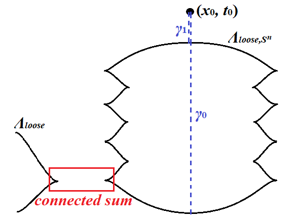
Figure 9. On the left there is the loose Legendrian $\Lambda_{\text{loose}}$ and on the right there is a loose Legendrian $\Lambda_{S^{n},\text{loose}}$ formally isotopic to the unknotted sphere (the front projection should be spinning around its symmetry axis). In the red region we perform the connected sum construction.

Proof.

We first construct a loose Legendrian sphere $\Lambda_{S^{n},\text{loose}}$ that is formally isotopic to the standard unknot sphere $\Lambda_{S^{n},\text{st}}$ and satisfies the properties in the lemma. Then we take a connected sum $\Lambda_{\text{loose}}\#\Lambda_{S^{n},\text{loose}}$. In fact, since $\Lambda_{\text{loose}}$ is compact, one can find $(x_{0},t_{0})\in\mathbb{R}^{n+1}$ such that there are no chords between $\Lambda^{\prime}_{\text{loose}}$ to $T_{(x_{0},t_{0})}^{*,\infty}\mathbb{R}^{n+1}$ (in other words the front projection of $\Lambda^{\prime}_{\text{loose}}$ is disjoint from the hypersurface $x=x_{0}$). We choose $\Lambda_{S^{n},\text{loose}}$ to be the Legendrian sphere in Figure 9, where the number of zigzags is to be determined. There are precisely 2 (transverse) Reeb chords $\gamma_{0},\gamma_{1}$ from $\Lambda^{\prime}_{\text{loose}}$ to $T_{(x_{0},t_{0})}^{*,\infty}\mathbb{R}^{n+1}$ and

$$l(\gamma_{0})-l(\gamma_{1})\geq A;$$

It is not hard to see that $\Lambda_{S^{n},\text{loose}}$ is formally isotopic to the standard unknot sphere $\Lambda_{S^{n},\text{st}}$ and the front projections of $\Lambda_{\text{loose}}$ and $\Lambda_{S^{n},\text{loose}}$ are separated by some hypersurface in $\mathbb{R}^{n+1}$. Therefore one can define the connected sum $\Lambda_{\text{loose}}\#\Lambda_{S^{n},\text{loose}}$ uniquely up to Legendrian isotopy [Rizconnectsum, Proposition 4.9].

We show that $\Lambda_{\text{loose}}\#\Lambda_{S^{n},\text{loose}}$ is formally isotopic to $\Lambda_{\text{loose}}$. This is because first $\Lambda_{S^{n},\text{loose}}$ is formally isotopic to $\Lambda_{S^{n},\text{st}}$ and this isotopy can be chosen to be fixed near the neighbourhood where the connected sum takes place. Second we perform a formal isotopy from $\Lambda_{\text{loose}}\#\Lambda_{S^{n},\text{st}}$ to $\Lambda_{\text{loose}}$. Since locally the connected sum is defined by connecting two cusps [Rizconnectsum, Section 4.2.2] (see Figure 9), one can explicitly see they are isotopic. This proves the claim. Hence by Murphy’s $h$-principle [Loose] $\Lambda_{\text{loose}}\#\Lambda_{S^{n},\text{loose}}$ is isotopic to $\Lambda_{\text{loose}}$.

This constructs $\Lambda^{\prime}_{\text{loose}}=\Lambda_{\text{loose}}\#\Lambda_{S^{n},\text{loose}}$ and by the construction of $\Lambda_{S^{n},\text{loose}}$ we know that condition (1) holds.

Now we show condition (2), that one can choose $\Lambda_{S^{n},\text{loose}}$ so that $\Lambda_{\text{loose}}\#\Lambda_{S^{n},\text{loose}}$ can be displaced from $T_{(x_{0},t_{0})}^{*,\infty}\mathbb{R}^{n+1}$ by a Hamiltonian $H_{s}\,(s\in I)$ with $\|H_{s}\|_{\text{osc}}\leq\epsilon$ so that there are no longer Reeb chords between them. This is because we can add sufficiently may zigzags in $\Lambda_{S^{n},\text{loose}}$ such that the derivatives of the front

$$\xi_{i}=\partial t/\partial x_{i}\in(-\epsilon/2n,\epsilon/2n),\,(1\leq i\leq n)$$

are sufficiently small, i.e. $\Lambda_{S^{n},\text{loose}}$ is contained in a neighbourhood of $\mathbb{R}^{n+1}\subset J^{1}(\mathbb{R}^{n})\subset T^{*,\infty}\mathbb{R}^{n+1}$. Then one can easily find a Hamiltonian $H_{s}\,(s\in I)$ supported in a neighbourhood $U_{\mathbb{R}^{n+1}}$ of $\mathbb{R}^{n+1}$ with $\|H_{s}\|_{\text{osc}}\leq\epsilon$ that displaces $\Lambda_{S^{n},\text{loose}}$ from $T_{(x_{0},t_{0})}^{*,\infty}\mathbb{R}^{n+1}$. For example, consider a cut-off function $\beta\in C^{\infty}(\mathbb{R})$ that is equal to $1$ in $(-\epsilon/2,\epsilon/2)$ and $0$ outside $(-\epsilon,\epsilon)$. Let $H(x,\xi,t)=\beta(|\xi|)\xi_{1}$, $\|H\|_{\text{osc}}\leq\epsilon$,

$$H|_{U_{\mathbb{R}^{n+1}}}=\xi_{1},\,\,X_{H}|_{U_{\mathbb{R}^{n+1}}}=-\partial/\partial x_{1}.$$

This will displace $\Lambda_{S^{n},\text{loose}}$ from $T_{(x_{0},t_{0})}^{*,\infty}\mathbb{R}^{n+1}$. ∎

Next we set up the foundation of the persistence module $\mathscr{H}om_{(-\infty,+\infty)}(\Bbbk_{(x_{0},t_{0})},\mathscr{F})$ in this case. Note that $\Bbbk_{(x_{0},t_{0})}\notin Sh_{\tau>0}^{b}(M\times\mathbb{R})$. However we claim that as long as $\mathscr{F}\in Sh_{\tau>0}^{b}(M\times\mathbb{R})$, all the arguments are still valid.

Lemma 7.3.

For $\Lambda\subset T^{*,\infty}_{\tau>0}(M\times\mathbb{R})$ and $\mathscr{F}\in Sh^{b}_{\Lambda}(M\times\mathbb{R})$,

$$SS^{\infty}(\mathscr{H}om((\Bbbk_{(x_{0},t_{0})})_{q},\mathscr{F}_{r}))\cap\mathrm{Graph}(du)=\emptyset.$$

On the other hand, there is an injection from

$$SS^{\infty}(\mathscr{H}om((\Bbbk_{(x_{0},t_{0})})_{q},\mathscr{F}_{r}))\cap\mathrm{Graph}(-du)$$

to the set of ordered Reeb chords (i.e. $u$ can be positive or negative) $\mathcal{Q}_{\pm}(T_{(x_{0},t_{0})}^{*,\infty}\mathbb{R}^{n+1},\Lambda)=\{c:[0,u]\rightarrow T^{*,\infty}_{\tau>0}\mathbb{R}^{n+1}\,|\,c(s)=(x,t+s,\xi,\tau),\,c(0)\in\Lambda,c(u)=(x_{0},t_{0},\xi,\tau)\}$.

The proof is identical as Lemma 4.1. Since this Lemma still holds, one can easily see that all discussions in Section 5 on the persistence structure still hold for the sheaf

$$\mathscr{H}om_{(-\infty,+\infty)}(\Bbbk_{(x_{0},t_{0})},\mathscr{F})=u_{*}\mathscr{H}om((\Bbbk_{(x_{0},t_{0})})_{q},\mathscr{F}_{r}).$$

Proof of Theorem 7.1.

First assume that $n\geq 2$. Suppose $\Lambda$ can be squeezed into a contact neighbourhood $U_{\text{loose}}$ of $\Lambda_{\text{loose}}$. By Lemma 7.2, we can apply a contact isotopy so that the contact neighbourhood $U_{\text{loose}}$ is mapped to a contact neighbourhood $U_{\text{loose}}^{\prime}$ of $\Lambda_{\text{loose}}^{\prime}$. Denote by $\Lambda^{\prime}$ the image of the original Legendrian submanifold in $U_{\text{loose}}^{\prime}$. By shrinking the contact neighbourhood $U_{\text{loose}}^{\prime}$ we may assume that for the projection $\pi_{\mathbb{R}^{n}}\circ\pi_{\text{front}}:U_{\text{loose}}^{\prime}\rightarrow\mathbb{R}^{n}$, the height of each connected component of $U_{\text{loose}}^{\prime}$ in the fiber of $\pi_{\mathbb{R}^{n}}\circ\pi_{\text{front}}$ is less than $\epsilon^{\prime}$ where $4\epsilon^{\prime}<A-\epsilon$.

Lemma 7.2 ensures that there exists $(x_{0},t_{0})\in\mathbb{R}^{n+1}$ such that there are precisely 2 transverse Reeb chords from $\Lambda_{\text{loose}}^{\prime}$ to $T_{(x_{0},t_{0})}^{*,\infty}\mathbb{R}^{n+1}$, starting from $(x_{0},t_{1})$ and $(x_{0},t_{2})$. For $\Lambda^{\prime}\subset U_{\text{loose}}^{\prime}$, since the mapping degree $[\Lambda^{\prime}]\neq 0\in H_{n}(\Lambda_{\text{loose}}^{\prime};\mathbb{Z}/2\mathbb{Z})$, the preimage of $(x_{0},t_{1})$ and $(x_{0},t_{2})$ under the projection $U_{\text{loose}}^{\prime}\rightarrow\Lambda_{\text{loose}}^{\prime}$ are $p_{1,1},...,p_{1,2k+1}$ and $p_{2,1},...,p_{2,2k+1}$, and

$$\min_{1\leq i,j\leq 2k+1}|u(p_{1,i})-u(p_{2,j})|\geq A-2\epsilon^{\prime}.$$

Consider the Hamiltonian $H_{s}\,(s\in I)$ with $\|H_{s}\|_{\text{osc}}\leq\epsilon+\epsilon^{\prime}<A-2\epsilon^{\prime}$ and horizontally displaces $\Lambda_{\text{loose}}^{\prime}$ from the cotangent fiber $T^{*,\infty}_{(x_{0},t_{0})}\mathbb{R}^{n+1}$ as in Lemma 7.2. For a sufficiently small neighbourhood $U_{\text{loose}}^{\prime}$ of $\Lambda_{\text{loose}}^{\prime}$, there will be a Hamiltonian $H_{s}\,(s\in I)$ with $\|H_{s}\|_{\text{osc}}\leq\epsilon+\epsilon^{\prime}$ that horizontally displaces $U_{\text{loose}}^{\prime}$. For $\mathscr{F}\in Sh_{\Lambda^{\prime}}(\mathbb{R}^{n+1})$ we calculate

$$\mathscr{H}om_{(-\infty,+\infty)}(\Bbbk_{(x_{0},t_{0})},\Phi_{H}^{s}(\mathscr{F})).$$

By Lemma 7.3, $u(p_{1,1}),...,u(p_{1,2k+1})$ and $u(p_{2,1}),...,u(p_{2,2k+1})$ correspond to all the starting points and ending points of the bars. In addition, for each point the number of bars $\Bbbk_{(a,b]}$ (either starting or ending there) in the sheaf is at least the rank of the microstalk of $\mathscr{F}$. Denote the rank of the microstalk of $\mathscr{F}$ by $2r+1$. We argue that there must be a bar starting from $u(p_{1,i})$ and ending at $u(p_{2,j})$. Otherwise all bars start at some $u(p_{1,i})$ will end at some $u(p_{1,j})$ for $i\neq j$. However, there are odd number of points $u(p_{1,1}),...,u(p_{1,2k+1})$, so there should be $(2r+1)(2k+1)/2$ bars connecting them, which leads to a contradiction.

Now that we know there is a bar starting from $u(p_{1,i})$ and ending at $u(p_{2,j})$, it will have length at least $A-2\epsilon^{\prime}$. By Theorem 5.5, under the Hamiltonian $H_{s}\,(s\in I)$ with $\|H_{s}\|_{\text{osc}}\leq\epsilon+\epsilon^{\prime}$, this bar will persist since $\epsilon+\epsilon^{\prime}<A-2\epsilon^{\prime}$. This leads to a contradiction.

Finally when $n=1$, we apply the spinning construction [EESNoniso, Section 4.4] (Figure 10) to a stablized Legendrian knot: namely consider a real line $t=t_{0}$ that is disjoint from the front projection $\Lambda_{\text{loose}}$, $\Lambda^{\prime}$ and spin around the front along the line $x=x_{0}$. The standard zigzag thus gives a loose chart for the new Legendrian $\Lambda_{\text{loose,spin}}$ and $\Lambda_{\text{spin}}^{\prime}$ in $T^{*,\infty}_{\tau>0}\mathbb{R}^{3}$. It is clear from the front projection that, if there is a sheaf with singular support on a knot, then there is also a sheaf with singular support on its spinning. In fact, we consider $\mathbb{R}^{3}\backslash\{(x,y,t)|x=x_{0},y=0\}\simeq\mathbb{R}^{2}\times S^{1}$ and the projection

$$\pi:\mathbb{R}^{3}\backslash\{(x,y,t)|x=x_{0},y=0\}\cong\mathbb{R}^{2}\times S^{1}\hookrightarrow\mathbb{R}^{3}.$$

Now take the sheaf $\pi^{-1}\mathscr{F}$ then $SS^{\infty}(\pi^{-1}\mathscr{F})=\Lambda_{\text{spin}}^{\prime}$. Note that $\mathrm{supp}(\mathscr{F})$ is compact, so $\pi^{-1}\mathscr{F}$ has zero stalk near the line $\{(x,y,t)|x=x_{0},y=0\}$ and we can easily extend it to a sheaf on $\mathbb{R}^{3}$. Then applying the argument above will complete the proof. ∎

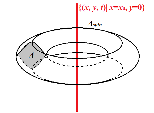
Figure 10. The front spinning of a standard unknot.