Chirped periodic and solitary waves in nonlinear negative index materials

Abstract

Propagation of ultrashort pulses at least a few tens of optical cycles in duration through a negative index material is investigated theoretically based on the generalized nonlinear Schrödinger equation with pseudo-quintic nonlinearity and self-steepening effect. Novel periodic waves of different forms are shown to exist in the system in the presence of higher-order effects. It is found that such periodic structures exhibit an interesting chirping property which depends on the light field intensity. The nonlinearity in pulse chirp is found to be caused by the presence of self-steepening effect in the negative index medium. The solutions also comprise dark, bright, and kink solitary waves. Stability of the solitary wave solutions are proved analytically using the theory of nonlinear dispersive waves. The stability of the solutions is numerically studied under finite initial perturbations.

I Introduction

Propagation of ultrashort light pulses in negative index materials (NIMs) has attracted considerable attention recently PLi -Shen . Such new materials are composed of a regular array of unit cells whose size is usually much smaller than the wavelengths of propagating electromagnetic waves PLi . Their remarkable property of having an antiparallel phase velocity and Poynting vector Pendry -Parazzoli , makes them the most potential candidates for stable soliton and other nonlinear phenomena Xiang1 . Compared with an ordinary material which is a medium possessing a constant permeability and positive refraction, a NIM has a dispersive permeability and a negative refraction. After the Veselago’s prediction Veselago and the experimental demonstration of NIMs Pendry1 ; Smith1 ; Smith2 , interest has been aroused in the study of the potential applications of such materials, which display properties beyond those available in naturally occurring materials. Further, experimental results have been recently obtained with studying nonlinear phenomena in NIMs, including parametric amplification Aguanno , modulation instability Popov , second-harmonic generation Wen , and soliton propagation Ban ; Boardman .

Theoretically, Scalora et al. Scalora have introduced a generalized nonlinear Schrödinger equation (NLSE) for a dispersive dielectric susceptibility and permeability appropriate for describing ultrashort pulse propagation in NIMs. This new NLSE model includes the contribution of higher-order effects such as pseudo-quintic nonlinearity and self-steepening effect with parameters directly related to the magnetic properties of the material. Development of such generalized NLSE was a great advance in the study of ultrashort electromagnetic pulses through NIMs. Subsequently, Zhang and Yi ZY obtained the exact chirped soliton solutions of this newly derived equation by employing the variable parametric method. Later, Marklund et al. Marklund also examined the modulational instability and localization of an ultrashort electromagnetic pulse that is governed by this generalized NLSE. Recently, Yang et al. Yang have discussed the existence of quasi-solitons within the framework of this generalized NLSE under the very specific condition of the vanishing self-steepening nonlinearity. As a particular result, they have obtained three types of exact bright, dark, bright-grey quasi-soliton solutions by employing the ansatz method. But with the increasing intensity of the optical field and further shortening of the pulses up to the femtosecond duration ($<100~{}\mathrm{fs}$), the self-steepening process becomes increasingly more important in optical systems Han . Such higher-order nonlinear effect is due to the intensity dependence of group velocity, which gives the optical pulse a very narrow width during the propagation Porsezian1 . It is worth noting that the presence of self-steepening process strongly affects the propagation of ultrashort pulses in nonlinear media. Thus, taking into account the contribution of this higher-order effect is relevant to understand experimental results and complement the previous studies. It should be mentioned that the addition of a higher-order nonlinear term to a given nonlinear evolution equation changes drastically it’s integrability properties.

Regarding the application of solitons, how to control the balance between nonlinear and dispersion effects becomes a significant subject in ultrafast optics Liu1 . In this context, new materials that can be successfully used for the generation of ultrashort pulses have been recently demonstrated Liu2 ; Liu3 . In addition, heterostructure materials having excellent optical properties in photonic device applications have been recently fabricated by employing the magnetron sputtering technique Liu4 . Theoretically, nonlinear control based on different dispersion and nonlinearity for third-order NLSE has been recently studied Liu5 . It is of interest to note that the investigation of soliton dynamics in the presence of higher-order effects has been also expanded into optical systems which are modeled by the complex cubic-quintic Ginzburg-Landau equation Liu6 ; Liu7 .

Interest in nonlinear periodic waves has grown rapidly in recent years due to their potential applications in many fields of physics Shamy -Lai . The study of such structures has made a remarkable progress because of their use in the nonlinear transport phenomenon Shamy . Note that cnoidal waves based on elliptic functions like $\mathrm{cn,}$ $\mathrm{sn}$ as well as $\mathrm{dn}$ are exact solutions in the form of periodic arrays of pulses. In optics, cnoidal (periodic) waves play a significant role in the analysis of the data transmission in fiber-optic telecommunications links D . Due to their structural stability with respect to the small input profile perturbations and collisions Petnikova , these propagating waves serve as a model of pulse train propagation in optics fibers D . In this context, we recently demonstrated the formation of periodic waves and localized pulses in an optical fiber medium under the influence of third-order dispersion and self-steepening effect, which can stably propagate through the system with a Kerr nonlinear response Vladimir . Although periodic waves have been widely studied in physical systems such as nonlinear optical fibers Vladimir ; Chow ; Chow1 and Bose-Einstein condensates FKh ; Chow2 , their investigation in NIMs has not been widespread. In addition, most previous studies on propagating periodic waves have been limited to the linearly chirped and chirp-free periodic structures Vladimir -Kruglov . An issue of great current interest is the search for periodic waves that are characterized by an enhanced nonlinearity in pulse chirp. From a practical stand point, chirped pulses are particularly useful in the design of optical devices such as fiber-optic amplifiers, optical pulse compressors and solitary wave based communication links Kruglov ; Desaix . In this paper, we study the formation of periodic waves in a NIM exhibiting pseudo-quintic nonlinearity and self-steepening effects. We find the periodic waves with these higher-order effects have a wide variety of functional forms with properties different from the ones existing in optical Kerr media. Importantly, the structures we obtained exhibit explicitly a nonlinear chirp that arises from the self-steepening process, and thus describe physically important applications as the compression and amplification of light pulses in negative index materials. Conditions for their existence as well as stability aspects of such privileged exact solutions are also investigated.

The paper is arranged as follows. In Sec. II, we briefly present the generalized NLSE describing ultrashort optical pulse propagation in a NIM and derive the nonlinear equation that governs the evolution of the light field intensity in the system. In Sec. III, we present results of novel chirped periodic solutions of the model and the nonlinear chirp associated with each of these structures. The solitary-wave (long-wave) limit of the periodic solutions is also considered here, which has given rise to localized pulses of bright, dark, gray, kink, and anti-kink type. In Sec. IV, the analytical stability analysis of chirped periodic and solitary wave solutions based on the theory of optical nonlinear dispersive waves is presented. In Sec. V, the the stability of the solutions is discussed numerically. The paper is concluded by Sec. VI (where, in particular, we present applications of the obtained periodic solutions in other systems such as nonlinear optical fibers).

II Traveling waves of generalized nonlinear Schrödinger equation

The governing equation for ultrashort pulse propagation in a negative index material with pseudo-quintic nonlinearity and self-steepening effect is given by the generalized NLSE Scalora :

$$i\frac{\partial\psi}{\partial z}+\frac{\sigma}{2}\frac{\partial^{2}\psi}{\partial t^{2}}+\rho\left|\psi\right|^{2}\psi-\epsilon\left|\psi\right|^{4}\psi-i\nu\frac{\partial}{\partial t}(\left|\psi\right|^{2}\psi)=0,$$ (1)

where $\psi\left(z,t\right)$ is the complex envelope of the electric field, with $z$ and $t$ the normalized propagation distance and time, respectively. The coefficient $\sigma=\left(1/\beta n\right)\left[1/V_{g}^{2}-\alpha\gamma-\beta\left(\varepsilon\gamma^{\prime}+\mu\alpha^{\prime}\right)/4\pi\right]$ denotes the group-velocity dispersion (GVD) parameter, $\rho=\beta\mu\chi^{(3)}/2n$ and $\epsilon=\beta\mu^{2}(\chi^{(3)})^{2}/8n^{3}$ are the cubic and pseudo-quintic nonlinearity coefficients, respectively, and $\nu=\chi^{(3)}[\mu/2V_{g}n^{2}-(\gamma+\mu)/2n]$ accounts for the pulse self-steepening effect. Here $\beta=2\pi\widetilde{\omega}=2\pi\omega/\omega_{p}$ where $\omega_{p}$ is the electric plasma frequency, $\chi^{(3)}$ is the third order susceptibility of the medium, $\mu$ is the effective magnetic permeability, $n$ is the refractive index, and $V_{g}=2n/\left(\varepsilon\gamma+\mu\alpha\right)$ is the group velocity of the pulse. Also $\alpha=\partial\left[\widetilde{\omega}\varepsilon(\widetilde{\omega})\right]/\partial\widetilde{\omega}$, $\alpha^{\prime}=\partial^{2}\left[\widetilde{\omega}\varepsilon(\widetilde{\omega})\right]/\partial\widetilde{\omega}^{2},$ $\gamma=\partial\left[\widetilde{\omega}\mu(\widetilde{\omega})\right]/\partial\widetilde{\omega}$, $\gamma^{\prime}=\partial^{2}\left[\widetilde{\omega}\mu(\widetilde{\omega})\right]/\partial\widetilde{\omega}^{2},$ where $\varepsilon$ and $\widetilde{\omega}$ denote dielectric susceptibility and normalized frequency, respectively. In what follows, we investigate the formation conditions and propagation properties of periodic and solitary waves and take the same values of the model parameters used in Ref. Yang . Such realistic parameter values are chosen depending on which ratio of $\omega_{m}/\omega_{p}$ is chosen to determine the engineered size of the constituents of NIM structures, the split-ring resonators, and so on (with $\omega_{m}$ is the magnetic plasma frequency). One should note that for categorizing the generalized NLSE to describe the behavior of negative refraction, it is further correlated with the lossless Drude model delineating the frequency dispersion with the permittivity and permeability of the form Scalora : $\varepsilon(\widetilde{\omega})=1-(1/(\widetilde{\omega}^{2}+i\widetilde{\omega}\gamma))$ and $\mu(\widetilde{\omega})=1-((\omega_{m}^{2}/\omega_{p}^{2})/(\widetilde{\omega}^{2}+i\widetilde{\omega}\gamma))$. Therefore, the refractive index of the medium defined by $n(\widetilde{\omega})=\pm\sqrt{\varepsilon(\widetilde{\omega})\mu(\widetilde{\omega})}$ is negative for $\widetilde{\omega}<0.8$ and positive for $\widetilde{\omega}>1.0$ if considering the typical value $\omega_{m}/\omega_{p}=0.8$ Yang ; Min . Following the expressions of the preceding parameters, for self-focusing nonlinearity, $\rho$ $>0$ and $\epsilon<0$ in the negative-index region $\widetilde{\omega}<0.8$, $\rho$ $>0$ and $\epsilon>0$ in the positive-index region $\widetilde{\omega}>1.0$; while for self-defocusing nonlinearity, $\rho$ $<0$ and $\epsilon<0$ in the negative index region and $\rho$ $<0$ and $\epsilon>0$ in the positive index region Yang . In addition, the sign of the GVD coefficient $\sigma$ can be positive or negative depending on the particular choice of parameters, and self-steepening characterizes the front of the pulse, unlike in the case of ordinary materials Scalora . One should also note that all the model parameters in the generalized NLSE (1) are function of the normalized frequency $\widetilde{\omega}$, whose specific dependence curves is depicted in figure 1 of Ref. Tsitsas . As stated in Refs. PLi ; Scalora ; Wen1 , the model parameters directly expressed by material permittivity and permeability $\varepsilon(\widetilde{\omega})$ and $\mu(\widetilde{\omega})$ can be tailored by engineering the unit-cell structure of  negative index materials, which implies more possibilities for the existence of wider classes of solitary waves Scalora .

Equation (1) for $\epsilon=0$ reduces to the derivative NLSE that describes the optical soliton propagation in the presence of Kerr dispersion Tzoar ; Anderson . As mentioned previously, exact bright, dark, bright-grey quasi-soliton solutions of Eq. (1) have been obtained under the special parametric condition $\nu=0$ in Yang . Here instead we shall analyze the existence of nonlinearly chirped periodic and solitary waves taking into account the influence of all effects on short-pulse propagation in the negative refractive index material.

In order to obtain the exact traveling-wave solutions of generalized NLSE (1), we consider a solution of the form,

$$\psi(z,t)=u(x)\exp[i\left(\kappa z-\delta t\right)+i\phi(x)],$$ (2)

where $u(x)$ and $\phi(x)$ are real functions depending on the variable $x=t-qz$, and $q=v^{-1}$ is the inverse velocity. Here $\kappa$ and $\delta$ are the corresponding real parameters describing the wave number and frequency shift. Equations (1) and (2) lead to the following system of the ordinary differential equations,

$$\frac{\sigma}{2}\left(u\frac{d^{2}\phi}{dx^{2}}+2\frac{d\phi}{dx}\frac{du}{dx}\right)-\left(q+\sigma\delta\right)\frac{du}{dx}-3\nu u^{2}\frac{du}{dx}=0,$$ (3)

$$\frac{\sigma}{2}\frac{d^{2}u}{dx^{2}}-\left(\kappa-q\frac{d\phi}{dx}\right)u-\frac{\sigma}{2}\left(\frac{d\phi}{dx}-\delta\right)^{2}u$$

$$+\nu\frac{d\phi}{dx}u^{3}+\left(\rho-\nu\delta\right)u^{3}-\epsilon u^{5}=0.$$ (4)

Multiplying Eq. (3) by the function $u(x)$ and integrating leads to the following equation,

$$\sigma u^{2}\frac{d\phi}{dx}-(q+\sigma\delta)u^{2}-\frac{3}{2}\nu u^{4}=K_{0},$$ (5)

where $K_{0}$ is the integration constant. We choose below $K_{0}=0$ then Eq. (5) yields,

$$\frac{d\phi}{dx}=\frac{q+\sigma\delta}{\sigma}+\frac{3\nu}{2\sigma}u^{2}.$$ (6)

The corresponding chirp $\Delta\omega$ defined as $\Delta\omega=-\partial\left[\kappa z-\delta t+\phi(x)\right]/\partial t$ is given by

$$\Delta\omega=-\frac{q}{\sigma}-\frac{3\nu}{2\sigma}u^{2}.$$ (7)

This result shows that the chirp is strongly dependent on the self-steepening parameter $\nu$ and varies with the wave intensity $\left|\psi\right|^{2}=u^{2}$. Accordingly, a nontrivial nature of the phase will take place, thus making the envelope pulses nonlinearly chirped. It is clear that this chirping property disappears in the absence of self-steepening effect (i.e., $\nu=0$), where only the unchirped pulses are allowed to exist in the negative index medium in the presence of the pseudo-quintic nonlinearity.

Further insertion of (6) into (4) gives to the following nonlinear ordinary differential equation,

$$\frac{d^{2}u}{dx^{2}}+au+bu^{3}+cu^{5}=0,$$ (8)

with the parameters $a,$ $b$ and $c$ given by

$$a=\frac{q^{2}+2\sigma\left(\delta q-\kappa\right)}{\sigma^{2}},~{}~{}~{}~{}b=\frac{2(\rho\sigma+\nu q)}{\sigma^{2}},~{}~{}~{}~{}c=\frac{3\nu^{2}-8\sigma\epsilon}{4\sigma^{2}}.$$ (9)

Integration of Eq. (8) yields the first order nonlinear differential equation,

$$\left(\frac{du}{dx}\right)^{2}+au^{2}+\frac{1}{2}bu^{4}+\frac{1}{3}cu^{6}=h_{0},$$ (10)

where $h_{0}$ is an integration constant. We define new function $Y(x)=u^{2}(x)$ which transforms Eq. (10) to the form,

$$\frac{1}{4\alpha_{0}}\left(\frac{dY}{dx}\right)^{2}=Y^{4}+\alpha_{3}Y^{3}+\alpha_{2}Y^{2}+\alpha_{1}Y,$$ (11)

with $\alpha_{0}=-c/3$, $\alpha_{3}=3b/2c$, $\alpha_{2}=3a/c$ and $\alpha_{1}=-3h_{0}/c$. We also define the polynomial $f(Y)$:

$$f(Y)=Y^{4}+\alpha_{3}Y^{3}+\alpha_{2}Y^{2}+\alpha_{1}Y=\prod_{i=1}^{4}(Y-Y_{i}),$$ (12)

where $Y_{i}$ are the roots of this polynomial. The previous equation (11) is a nonlinear ordinary differential equation, which governs the evolution of the wave intensity as it propagates through the negative refractive index material. It gives a complete description of the envelope dynamics in NIMs under the influence of higher-order effects such as pseudoquintic nonlinearity and self-steepening effect. The general solution of Eq. (11) has the form,

$$\pm\int\frac{dY}{\sqrt{\mathrm{sgn}(\alpha_{0})(Y^{4}+\alpha_{3}Y^{3}+\alpha_{2}Y^{2}+\alpha_{1}Y)}}=2\sqrt{|\alpha_{0}|}(x-\eta),$$ (13)

where $\mathrm{sgn}(\alpha_{0})=\alpha_{0}/|\alpha_{0}|$ for $\alpha_{0}\neq 0$, and $\eta$ is an integration constant. We consider in the following section different cases which yield the periodic bounded and solitary wave solutions of the generalized NLSE (1).

III Chirped periodic and solitary wave solutions

We consider here the particular case with real roots for equation $f(Y)=0$ and $\alpha_{0}=-c/3>0$. Let all roots are different then we can select them as $Y_{1}>Y_{2}>Y_{3}>Y_{4}$. We consider the case when function $Y(x)$ belongs to the next interval $Y_{2}\geq Y\geq Y_{3}$. The integral in Eq. (13) for real roots $Y_{i}$ with $Y_{1}>Y_{2}>Y_{3}>Y_{4}$ and $Y_{2}\geq Y\geq Y_{3}$ can be written in the next form,

$$\int_{Y}^{Y_{2}}\frac{dY^{\prime}}{\sqrt{(Y^{\prime}-Y_{1})(Y^{\prime}-Y_{2})(Y^{\prime}-Y_{3})(Y^{\prime}-Y_{4})}}=\frac{2F(s;k)}{\sqrt{(Y_{1}-Y_{3})(Y_{2}-Y_{4})}},$$ (14)

where the parameters $s$ and $k$ are given by

$$s=\left(\frac{(Y_{1}-Y_{3})(Y_{2}-Y)}{(Y_{2}-Y_{3})(Y_{1}-Y)}\right)^{1/2},~{}~{}~{}~{}k=\left(\frac{(Y_{2}-Y_{3})(Y_{1}-Y_{4})}{(Y_{1}-Y_{3})(Y_{2}-Y_{4})}\right)^{1/2}.$$ (15)

The function $F(s;k)$ is Jacoby form of the elliptic integral of the first kind,

$$F(s;k)=\int_{0}^{s}\frac{dx}{\sqrt{(1-x^{2})(1-k^{2}x^{2})}}.$$ (16)

Equations (13) and (14) lead the following relation,

$$\frac{(Y_{1}-Y_{3})(Y_{2}-Y(x))}{(Y_{2}-Y_{3})(Y_{1}-Y(x))}=\mathrm{sn}^{2}(w(x-\eta),k),$$ (17)

where $\mathrm{sn}(z,k)$ is the Jacoby elliptic function ($0\leq k\leq 1$) and the parameter $w$ is given by

$$w=\sqrt{\alpha_{0}(Y_{1}-Y_{3})(Y_{2}-Y_{4})},$$ (18)

with $\alpha_{0}>0$. Equation (17) yields the periodic bounded solution for the function $u(x)$ when the parameter $k$ in Eq. (15) belongs to the interval $0<k<1$. This periodic bounded solutions are given by

$$u(x)=\pm\sqrt{\frac{Y_{2}-Y_{1}\Lambda\mathrm{sn}^{2}(w(x-\eta),k)}{1-\Lambda\mathrm{sn}^{2}(w(x-\eta),k)}},~{}~{}~{}~{}\Lambda=\frac{Y_{2}-Y_{3}}{Y_{1}-Y_{3}}.$$ (19)

We show below that this periodic solution reduces to soliton solution when the parameter $k=1$. The period $T$ of this bounded periodic solution is $T=(2/w)K(k)$ where the function $K(k)$ is given by

$$K(k)=\int_{0}^{1}\frac{dx}{\sqrt{(1-x^{2})(1-k^{2}x^{2})}}=F(1;k).$$ (20)

The nonlinearity in pulse chirp is caused by the presence of self-steepening effect in the negative index medium. A rich variety of nonlinearly chirped solitary waves are obtained in the long-wave limit of the derived periodic waves. The solutions contain dark, bright, and kink solitary wave solutions, demonstrating the structural diversity of localized waves in the material. We show below that the general solutions in Eqs. (13) and (19) lead to different periodic and solitary wave solutions of the generalized NLSE (1).

1. Periodic bounded waves

We have found a family of nonlinearly chirped periodic bounded solutions by Eqs. (2) and (19) as

$$\psi(z,t)=\pm\sqrt{\frac{Y_{2}-Y_{1}\Lambda\mathrm{sn}^{2}(w\xi,k)}{1-\Lambda\mathrm{sn}^{2}(w\xi,k)}}\exp[i\left(\kappa z-\delta t\right)+i\phi(x)],$$ (21)

where $\xi=t-qz-\eta$, parameter $k$ ($0<k<1$) is given by Eq. (15), and parameter $w$ is defined by Eq. (18) with $\alpha_{0}=-c/3>0$. The phase $\phi(x)$ in this solution is following by Eq. (6) as

$$\phi(x)=\left(\frac{q}{\sigma}+\delta\right)(x-\eta)+\frac{3\nu}{2\sigma}\int_{\eta}^{x}u^{2}(x^{\prime})dx^{\prime}+\phi_{0},$$ (22)

which shows that under the influence of self-steepening nonlinearity, the propagating waveforms acquires an extra characteristic phase $\phi(x)$ which depends on the squared amplitude of the complex envelope and varies with the self-steepening parameter $\nu$. To be specific, in the presence of self-steepening effect, the phase (22) takes a nontrivial structure leading to chirped pulses. Obviously, in the limit of $\nu=0$ (that is, at a vanishing self-steepening effect), the phase distribution becomes a linear function of $\xi$.

Equation (15) yields $k=1$ in the limiting case $Y_{3}=Y_{4}$. Note that function $f(Y)$ has at least one root equal to zero. Thus in the limiting case with $k=1$ we have $Y_{3}=Y_{4}=0$ and the parameter $\alpha_{1}=0$. Hence the case with $k=1$ occurs when the integration constant $h_{0}=0$. In this limiting case, the periodical solution in Eq. (19) reduces to soliton solution as

$$u(x)=\pm\sqrt{\frac{Y_{2}[1-\mathrm{tanh}^{2}(w\xi)]}{1-(Y_{2}/Y_{1})\mathrm{tanh}^{2}(w\xi)}},$$ (23)

where $w=\sqrt{-(c/3)Y_{1}Y_{2}}$ and $Y_{1}$ and $Y_{2}$ are the roots of equation $Y^{2}+\alpha_{3}Y+\alpha_{2}=0$. One can also write this solution in the next equivalent form,

$$u(x)=\frac{\pm\sqrt{Y_{1}}}{\sqrt{1+[(Y_{1}/Y_{2})-1]\mathrm{cosh}^{2}(w\xi)}},$$ (24)

where $Y_{1}>Y_{2}$. The roots $Y_{1}$ and $Y_{2}$ are given by

$$Y_{1}=\frac{3b+\sqrt{3(3b^{2}-16ac)}}{4|c|},~{}~{}~{}~{}Y_{2}=\frac{3b-\sqrt{3(3b^{2}-16ac)}}{4|c|}.$$ (25)

One can also write the soliton solution given in Eq. (24) as

$$u(x)=\frac{A}{\sqrt{1+B\mathrm{cosh}(w_{0}\xi)}},$$ (26)

where $\xi=t-qz-\eta$, and the parameters $A$, $B$, and $w_{0}$ are

$$A=\pm\sqrt{\frac{2Y_{1}Y_{2}}{Y_{1}+Y_{2}}}=\pm 2\sqrt{-\frac{a}{b}},$$ (27)

$$B=\frac{Y_{1}-Y_{2}}{Y_{1}+Y_{2}}=\sqrt{1-\frac{16ac}{3b^{2}}},$$ (28)

$$w_{0}=\sqrt{-(c/3)Y_{1}Y_{2}}=2\sqrt{-a},$$ (29)

with $a<0$, $b>0$, and $3b^{2}>16ac$.

2. Bright solitary waves

Substitution of (26) into (2) yields to the following exact chirped bright solitary wave solution of Eq. (1) as

$$\psi(z,t)=\frac{A}{\sqrt{1+B\cosh(w_{0}\xi)}}\exp[i\left(\kappa z-\delta t\right)+i\phi(x)],$$ (30)

with $a<0$, $b>0$, and $3b^{2}>16ac$. Here $\xi=t-qz-\eta$, and the parameters $A$, $B$, and $w_{0}$ are given in Eqs. (27), (28) and (29) respectively. The phase $\phi(x)$ is evaluated by Eqs. (22) and (26) as

$$\phi(x)=\frac{3\nu A^{2}}{\sigma w_{0}D}\mathrm{arctanh}\left(\frac{D}{1+B}~{}\mathrm{tanh}\left(\frac{1}{2}w_{0}(x-\eta)\right)\right)$$

$$+\left(\frac{q}{\sigma}+\delta\right)(x-\eta)+\phi_{0},~{}~{}~{}~{}~{}~{}~{}~{}~{}~{}~{}~{}~{}~{}~{}~{}~{}~{}$$ (31)

where $\phi_{0}$ is integration constant and the parameter $D$ is

$$D=\sqrt{1-B^{2}}=\sqrt{\frac{16ac}{3b^{2}}}.$$ (32)

Note that $D$ is real and $D\neq 0$ when $c<0$ because in this soliton solution $a<0$.

Figure 1: (a) Intensity profile of the chirped bright solitary wave $\left|\psi(0,t)\right|^{2}$ as a function of $t$ and its (b) evolution as computed from Eq. (30) for the values $\sigma=-0.1990,$ $\rho=-5.0265\times 10^{-10},$ $\epsilon=3.3511\times 10^{-20},$ $\nu=-6.2918\times 10^{-14},$ $q=0.5,$ $\kappa=0.257,$ $\eta=0,$ and $\delta=1.82$. Here the solitary wave intensity is normalized by $\left|\psi(z,t)\right|^{2}/A^{2}.$

We have shown the solitary wave profile and its evolution in Figs. 1(a) and 1(b) respectively, for the parameter values Yang : $\sigma=-0.1990,$ $\rho=-5.0265\times 10^{-10},$ $\epsilon=3.3511\times 10^{-20},$ and $\nu=-6.2918\times 10^{-14}$. Other parameters are $q=0.5,$ $\kappa=0.257,$ $\eta=0,$ and $\delta=1.82$. It is clearly seen that this nonlinearly chirped bright pulse propagate on a zero background in the negative index medium in the presence of various physical effects. This demonstrated that bright-type solitary waves that are characterized by a nonlinear chirp can exist in the system and the formation of these structures is strongly depends on all the material parameters.

3. Periodic waves connected to bright solitary waves

The soliton solution in Eq. (30) is connected with the special periodic solution when $a>0$, $b<0$, and $3b^{2}>16ac$. We have found such an exact periodic wave solution of Eq. (8) as $u(x)=A[1+B\cos(w(x-\eta))]^{-1/2}$. In this case, the chirped periodic solution of Eq. (1) has the form,

$$\psi(z,t)=\frac{A}{\sqrt{1+B\cos(w(x-\eta))}}\exp[i\left(\kappa z-\delta t\right)+i\phi(x)],$$ (33)

where $x=t-qz$, and the parameters $A$, $B$, and $w$ are given by

$$A^{2}=-\frac{4a}{b},~{}~{}~{}~{}B=\pm\sqrt{1-\frac{16ac}{3b^{2}}},~{}~{}~{}~{}w=2\sqrt{a}.$$ (34)

Hence the periodic solution in Eq. (33) is bounded when $a>0$, $b<0$, $3b^{2}>16ac$, and $|B|<1$. The phase $\phi(x)$ is evaluated by Eqs. (22) and (33) as

$$\phi(x)=\frac{3\nu A^{2}}{\sigma wD}\mathrm{arctan}\left(\frac{D}{1+B}~{}\mathrm{tan}\left(\frac{1}{2}w(x-\eta)\right)\right)$$

$$+\left(\frac{q}{\sigma}+\delta\right)(x-\eta)+\phi_{0},~{}~{}~{}~{}~{}~{}~{}~{}~{}~{}~{}~{}~{}~{}~{}~{}~{}~{}$$ (35)

where $\phi_{0}$ is integration constant and $D=\sqrt{1-B^{2}}=\sqrt{16ac/3b^{2}}$. Note that $D$ is real and $D\neq 0$ when $c>0$ because in this periodic solution $a>0$.

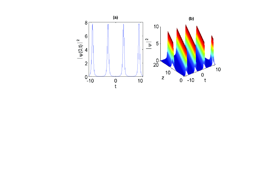
Figure 2: (a) Intensity profile of the chirped periodic wave $\left|\psi(0,t)\right|^{2}$ as a function of $t$ and its (b) evolution as computed from Eq. (33) for the values $\rho=5.0265\times 10^{-10},$ $\kappa=0.15,$ and $\delta=1.5.$ Other parameters are same as given in Fig. 1, and the solitary wave intensity is normalized by $\left|\psi(z,t)\right|^{2}/A^{2}$.

Figure 2(a) depicts the intensity profile of the chirped periodic wave solution (33) for the parameter values $\sigma=-0.1990,$ $\rho=5.0265\times 10^{-10},$ $\epsilon=3.3511\times 10^{-20},$ $\nu=-6.2918\times 10^{-14}$, $q=0.5,$ $\kappa=0.15,$ $\eta=0,$ and $\delta=1.5$, while Fig. 2(b) illustrates its evolution. One observes that the nonlinear waveform presents an oscillating behavior as it propagates through the negative index material.

4. Dark solitary waves

We have found a dark solitary wave as

$$u(x)=\frac{A\tanh(w_{0}(x-\eta))}{\sqrt{1+B~{}{\mathrm{sech}}^{2}(w_{0}(x-\eta))}}.$$ (36)

In this dark soliton solution, the parameters $A$, $B$ and $w_{0}$ are given by

$$A^{2}=-\frac{b}{2c}\pm\frac{1}{2c}\sqrt{b^{2}-4ac},$$ (37)

$$B=\frac{2a+2bA^{2}}{4a+bA^{2}},~{}~{}~{}~{}w_{0}=\sqrt{a+\frac{1}{2}bA^{2}},$$ (38)

with $b^{2}-4ac>0$, $A^{2}>0$, $B>-1$ and $a+\frac{1}{2}bA^{2}>0$. Note that we have the following equation for parameter $A$: $a+bA^{2}+cA^{4}=0$. Inserting (36) into (2), we get an exact nonlinearly chirped dark solitary wave solution for Eq. (1) in the form,

$$\psi(z,t)=\frac{A\tanh(w_{0}(x-\eta))}{\sqrt{1+B{\mathrm{sech}}^{2}(w_{0}(x-\eta))}}\exp[i\left(\kappa z-\delta t\right)+i\phi(x)].$$ (39)

The phase function $\phi(x)$ is given by Eq. (22) and Eq. (36) as

$$\phi(x)=\frac{3\nu A^{2}C}{4\sigma w_{0}}\ln\left(\frac{C-\tanh(w_{0}\xi)}{C+\tanh(w_{0}\xi)}\right)$$

$$+\left(\frac{q}{\sigma}+\delta\right)(x-\eta)+\phi_{0},~{}~{}~{}~{}~{}~{}~{}~{}~{}~{}~{}~{}~{}~{}~{}~{}~{}~{}$$ (40)

where the parameter $C$ has the form,

$$C=\sqrt{1+\frac{1}{B}}=\sqrt{\frac{6a+3bA^{2}}{2a+2bA^{2}}}.$$ (41)

It is worth mentioning that the solution (39) exists under the following conditions,

$$b^{2}-4ac>0,~{}~{}~{}~{}A^{2}=-\frac{b}{2c}\pm\frac{1}{2c}\sqrt{b^{2}-4ac}>0,$$ (42)

$$\frac{2a+2bA^{2}}{4a+bA^{2}}>-1,~{}~{}~{}~{}a+\frac{1}{2}bA^{2}>0.$$ (43)

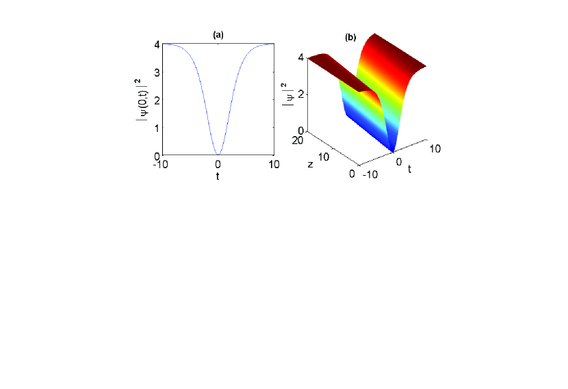
Figure 3: (a) Intensity profile of the chirped dark solitary wave $\left|\psi(0,t)\right|^{2}$ as a function of $t$ and its (b) evolution as computed from Eq. (39) for the values $\sigma=-0.7954,$ $\rho=1.2566\times 10^{-10},$ $\epsilon=2.095\times 10^{-21},$ $\nu=-4.8195\times 10^{-14},$ $q=0.1,$ $\kappa=0.2931,\eta=0,$ and $\delta=2$ . Here the solitary wave intensity is normalized by $\left|\psi(z,t)\right|^{2}/A^{2}$.

The intensity profile and evolution of the chirped solitary wave solution (39) in NIMs are shown in Figs. 3(a) and 3(b) respectively. Here we have taken the parameter values as Yang : $\sigma=-0.7954,$ $\rho=1.2566\times 10^{-10},$ $\epsilon=2.095\times 10^{-21},$ and $\nu=-4.8195\times 10^{-14}$. Other parameters are $q=0.1,$ $\kappa=0.2931,\eta=0,$ and $\delta=2$. It can be seen from Fig. 3 that under the influence of higher-order effects such as pseudo-quintic nonlinearity and self-steepening effect, the dark-type solitary waves with a nonlinear chirp may exist in NIMs.

5. Periodic waves connected to dark solitary waves

The dark solitary wave in Eq. (36) is connected with the special periodic solution. We have found such an exact periodic wave solution of Eq. (8) as

$$u(x)=\frac{A\sin(w(x-\eta))}{\sqrt{B+\cos^{2}(w(x-\eta))}}.$$ (44)

In this closed form solution, the parameters $A$, $B$ and $w$ are defined by the relations,

$$A^{2}=\frac{b}{2c}\pm\frac{1}{2c}\sqrt{b^{2}-4ac},$$ (45)

$$B=\frac{-2a+2bA^{2}}{-4a+bA^{2}},~{}~{}~{}~{}w=\sqrt{-a+\frac{1}{2}bA^{2}},$$ (46)

with $b^{2}-4ac>0$, $A^{2}>0$, $B>0$ and $-a+\frac{1}{2}bA^{2}>0$. Note that amplitude $A$ satisfies the equation $cA^{4}-bA^{2}+a=0$. Inserting (44) into (2), we get a chirped periodic wave solution for Eq. (1) in the form,

$$\psi(z,t)=\frac{A\sin(w(x-\eta))}{\sqrt{B+\cos^{2}(w(x-\eta))}}\exp[i\left(\kappa z-\delta t\right)+i\phi(x)].$$ (47)

The phase function $\phi(x)$ follows by Eq. (22) and Eq. (44) as

$$\phi(x)=\frac{3\nu A^{2}}{2\sigma w}\sqrt{\frac{B+1}{B}}~{}\mathrm{arctan}\left(\sqrt{\frac{B}{B+1}}~{}\mathrm{tan}\left(w(x-\eta)\right)\right)$$

$$+\left(\frac{q}{\sigma}+\delta-\frac{3\nu A^{2}}{2\sigma}\right)(x-\eta)+\phi_{0}.~{}~{}~{}~{}~{}~{}~{}~{}~{}~{}~{}~{}~{}~{}~{}~{}~{}~{}$$ (48)

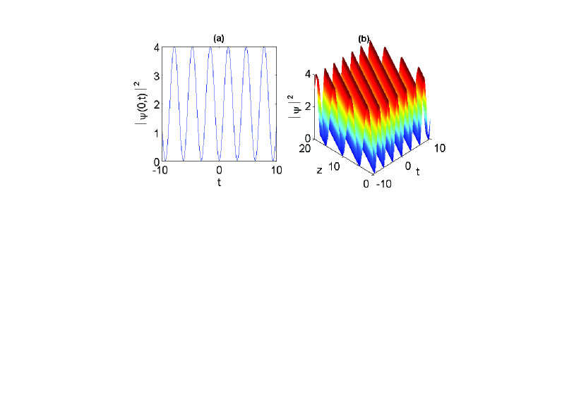
Figure 4: (a) Intensity profile of the chirped periodic wave $\left|\psi(0,t)\right|^{2}$ as a function of $t$ and its (b) evolution as computed from Eq. (47) for the values $\rho=-1.2566\times 10^{-10},$ $\kappa=0.15,$ and $\delta=2.5571$. Other parameters are same as given in Fig. 3, and the solitary wave intensity is normalized by $\left|\psi(z,t)\right|^{2}/A^{2}$.

An example of the intensity profile and evolution of the chirped periodic solution (47) is shown in Figs. 4(a) and 4(b) respectively, for the parameter values: $\sigma=-0.7954,$ $\rho=-1.2566\times 10^{-10},$ $\epsilon=2.095\times 10^{-21},$ $\nu=-4.8195\times 10^{-14},$ $q=0.1,$ $\kappa=0.15,\eta=0,$ and $\delta=2.5571$.

6. Gray solitary waves

We have also found an exact solution for Eq. (18) of the form,

$$u(x)=\frac{A}{\sqrt{1+B~{}{\tanh}^{2}(w_{0}(x-\eta))}},$$ (49)

where

$$B=\lambda-3\pm\sqrt{\lambda(\lambda-3)},~{}~{}~{}~{}\lambda=\frac{3b^{2}}{4ac},$$ (50)

$$A^{2}=-\frac{3b(B+1)}{2c(B+3)},~{}~{}~{}~{}w_{0}=\sqrt{\frac{aB}{3+2B}},$$ (51)

with the requirement as $B>-1$, $\lambda(\lambda-3)>0$, $bc<0$ and $aB>0$. Note that the parameter $B$ satisfies the equation $(B+3)^{2}=\lambda(2B+3)$. Thus in the general case, we have $B>-1$ and we obtain a gray solitary wave solution (i.e., a dark pulse with a nonzero minimum in intensity) as

$$\psi(z,t)=\frac{A}{\sqrt{1+B~{}{\tanh}^{2}(w_{0}(x-\eta))}}\exp[i(\kappa z-\delta t)+i\phi(x)].$$ (52)

The phase $\phi(x)$ given in Eq. (52) for the case $-1<B<0$ is

$$\phi(x)=\frac{3\nu A^{2}\sqrt{-B}}{4\sigma w_{0}(1+B)}\ln\left(\frac{1-\sqrt{-B}\tanh(w_{0}(x-\eta))}{1+\sqrt{-B}\tanh(w_{0}(x-\eta))}\right)$$

$$+\left(\delta+\frac{q}{\sigma}+\frac{3\nu A^{2}}{2\sigma(1+B)}\right)(x-\eta)+\phi_{0}.~{}~{}~{}~{}~{}~{}~{}~{}~{}~{}~{}~{}~{}~{}$$ (53)

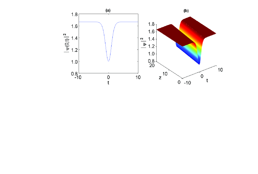
Figure 5: (a) Intensity profile of the chirped gray solitary wave $\left|\psi(0,t)\right|^{2}$ as a function of $t$ and its (b) evolution as computed from Eq. (52) for the values $\rho=-1.2566\times 10^{-10},$ $\epsilon=-2.095\times 10^{-21},$ $\kappa=0.15,$ $B=-0.4,$ and $\delta=20.0581.$ Other parameters are same as given in Fig. 3, and the solitary wave intensity is normalized by $\left|\psi(z,t)\right|^{2}/A^{2}$.

Figures 5(a) and 5(b) illustrate the intensity profile and evolution of the chirped solitary wave solution (52). Here the used parameter values: $\sigma=-0.7954,$ $\rho=-1.2566\times 10^{-10},$ $\epsilon=-2.095\times 10^{-21},$ $\nu=-4.8195\times 10^{-14}$, $q=0.1,$ $\kappa=0.15,$ $B=-0.4,$ $\eta=0,$ and $\delta=20.0581$.

7. Periodic waves connected to gray solitary waves

The gray solitary wave in Eq. (49) is connected with the special periodic solution. We have found such an exact periodic wave solution of Eq. (8) in the form,

$$u(x)=\frac{A}{\sqrt{1+B~{}\tan^{2}(w(x-\eta))}},$$ (54)

where

$$B=3-\lambda\pm\sqrt{\lambda(\lambda-3)},~{}~{}~{}~{}\lambda=\frac{3b^{2}}{4ac},$$ (55)

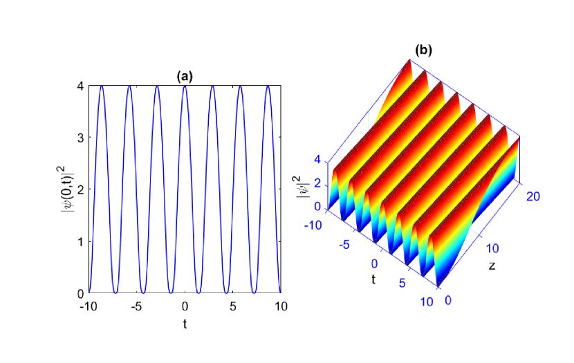
Figure 6: (a) Intensity profile of the chirped periodic wave $\left|\psi(0,t)\right|^{2}$ as a function of $t$ and its (b) evolution as computed from Eq. (57) for the values $\kappa=1.865,$ $B=0.4,$ and $\delta=0.314.$ Other parameters are same as given in Fig. 3, and the solitary wave intensity is normalized by $\left|\psi(z,t)\right|^{2}/A^{2}$.

$$A^{2}=-\frac{3b(1-B)}{2c(3-B)},~{}~{}~{}~{}w=\sqrt{\frac{aB}{3-2B}},$$ (56)

with the requirement $B>0$, $\lambda(\lambda-3)>0$, $bc(1-B)(3-B)<0$ and $a(3-2B)>0$. Note that the parameter $B$ satisfies the equation $(3-B)^{2}=\lambda(3-2B)$.

Thus we obtain a chirped periodic wave solution of Eq. (1) as

$$\psi(z,t)=\frac{A}{\sqrt{1+B~{}{\tan}^{2}(w(x-\eta))}}\exp[i(\kappa z-\delta t)+i\phi(x)].$$ (57)

The phase $\phi(x)$ follows by Eq. (22) and Eq. (54) as

$$\phi(x)=\frac{3\nu A^{2}\sqrt{B}}{2\sigma w\left(B-1\right)}~{}\mathrm{arctan}\left[\sqrt{B}~{}\mathrm{tan}\left(w(x-\eta)\right)\right]$$

$$+\left(\frac{q}{\sigma}+\delta+\frac{3\nu A^{2}}{2\sigma\left(1-B\right)}\right)(x-\eta)+\phi_{0}.~{}~{}~{}~{}~{}~{}~{}~{}~{}~{}~{}~{}~{}~{}~{}$$ (58)

The profile and evolution of the chirped periodic wave solution (57) are shown in Figs. 6(a) and 6(b), respectively. Here we have taken the  parameter values Yang : $\sigma=-0.7954,$ $\rho=1.2566\times 10^{-10},$ $\epsilon=2.095\times 10^{-21},$ and $\nu=-4.8195\times 10^{-14}$. Other parameters are $q=0.1,$ $\kappa=1.865,$ $B=0.4,$ $\eta=0,$ and $\delta=0.314$.

8. Kink-type solitary waves

The solution of Eq. (18), in particular case when $3b^{2}/16ac=1$, can be written in the form,

$$u(x)=A\sqrt{1\pm{\tanh}(w_{0}(x-\eta))},$$ (59)

where

$$A^{2}=-\frac{2a}{b},~{}~{}~{}~{}w_{0}=\sqrt{-a},$$ (60)

with conditions $a<0$ and $b>0$. Thus the chirped kink-type solitary wave solution of Eq. (1) is

$$\psi(z,t)=A\sqrt{1\pm{\tanh}(w_{0}(x-\eta))}\exp[i(\kappa z-\delta t)+i\phi(x)].$$ (61)

In this case, the phase function $\phi(x)$ is given by Eq. (22) and Eq. (59) as

$$\phi(x)=\pm\frac{3\nu A^{2}}{2\sigma w_{0}}\ln[\cosh(w_{0}(x-\eta))]$$

$$+\left(\delta+\frac{q}{\sigma}+\frac{3\nu A^{2}}{2\sigma}\right)(x-\eta)+\phi_{0}.$$ (62)

Figures 7(a) and 7(b) depict the evolution of the intensity wave profile of kink-shaped (upper sign) and anti-kink-shaped (lower sign) solitary waves as computed from Eq. (61) for the same parameter values $\sigma=-0.7954,$ $\rho=-1.2566\times 10^{-10},$ $\epsilon=-2.095\times 10^{-21},$ and $\nu=-4.8195\times 10^{-14}$. Other parameters are $q=0.1,$ $\kappa=1.2,\eta=0,$ and $\delta=26.1937$.

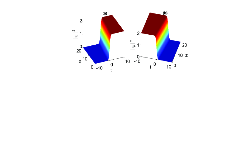
Figure 7: (a) Intensity profile of the chirped kink-type solitary wave $\left|\psi(0,t)\right|^{2}$ as a function of $t$ and its (b) evolution as computed from Eq. (61) for the values $\rho=-1.2566\times 10^{-10},$ $\epsilon=-2.095\times 10^{-21},$ $\kappa=1.2,$ and $\delta=26.1937.$ Other parameters are same as given in Fig. 3, and the solitary wave intensity is normalized by $\left|\psi(z,t)\right|^{2}/A^{2}$.

IV Stability analysis of periodic and solitary waves

We consider in this section the analytical stability analysis of soliton solutions and periodic waves for the generalized NLSE (1). Our approach is based on the theory of nonlinear dispersive waves in nonlinear optics and fluid dynamics Vladimir ; KrTr ; TK ; Whit . For our purpose, we develop the dynamics of dispersive waves in the following form,

$$\psi(z,t)=F(\Delta\omega)\exp[i\Theta(z,t)],$$ (63)

where the amplitude $F(\Delta\omega)$ and phase $\Theta(z,t)$ are real functions, and $\Delta\omega(z,t)$ is the frequency shift of nonlinear dispersive wave. It is worth noting that $\psi(z,t)$ is slowly varying amplitude for the pulse envelope. Hence the frequency of nonlinear dispersive wave is $\omega_{0}+\Delta\omega$ where $\omega_{0}$ is the carrier frequency. However, we use in this section more simple notation $\Delta\omega(z,t)\equiv\omega(z,t)$ for the frequency shift of the dispersive waves. Hence, the amplitude in Eq. (63) is $F(\omega)$, and the wave number shift $k$ and frequency shift $\omega$ of nonlinear dispersive waves are

$$k(\omega)=\frac{\partial\Theta}{\partial z},~{}~{}~{}~{}\omega=-\frac{\partial\Theta}{\partial t}.$$ (64)

We have by definition that $\Theta_{zt}=k_{t}$ and $\Theta_{tz}=-\omega_{z}$ which yield the equation,

$$\frac{\partial\omega}{\partial z}+\frac{\partial k(\omega)}{\partial t}=0.$$ (65)

We assume in our approach that $\omega(z,t)=\tilde{\omega}(Z,T)$ and $k(z,t)=\tilde{k}(Z,T)$ where $Z=\varepsilon z$ and $T=\varepsilon t$ with $\varepsilon\ll 1$ are slow variables. Here $\tilde{\omega}(Z,T)$ and $\tilde{k}(Z,T)$ are slow varying functions of variables $Z$ and $T$.

Thus this approach to stability analysis of solitons and periodic waves Vladimir ; KrTr ; TK is based on the method of slow variables. Note that the generalized NLSE (1) is derived in quasi-monochromatic approximation assuming that the parameter $\varepsilon\equiv\Delta\omega_{s}/\omega_{0}$ is small ($\varepsilon\ll 1$). Here $\Delta\omega_{s}$ and $\omega_{0}$ are the spectral width of the pulse and the carrier frequency respectively. Hence the condition $\varepsilon\ll 1$ is satisfied for the generalized NLSE (1). The substitution of Eq. (63) (with $\Delta\omega\equiv\omega$) into the generalized NLSE (1) leads to series of nonlinear equations. The equation in zero order to small parameter $\varepsilon$ is

$$k(\omega)=k_{0}(\omega)+\Gamma(\omega)F^{2}(\omega)-\epsilon F^{4}(\omega),$$ (66)

where $k_{0}(\omega)$ and $\Gamma(\omega)$ are

$$k_{0}(\omega)=-\frac{\sigma}{2}\omega^{2},~{}~{}~{}~{}\Gamma(\omega)=\rho-\nu\omega.$$ (67)

The parameter $\Gamma(\omega)$ is nonlinear coefficient renormalized by self-steepening effect. Equations (1), (63), (64) in the first order to small parameter $\varepsilon$ yield

$$\frac{\partial F}{\partial z}+k_{0}^{{}^{\prime}}(\omega)\frac{\partial F}{\partial t}=-\frac{1}{2}k_{0}^{{}^{\prime\prime}}(\omega)F\frac{\partial\omega}{\partial t}+3\nu F^{2}\frac{\partial F}{\partial t},$$ (68)

with $k_{0}^{{}^{\prime}}(\omega)=dk_{0}(\omega)/d\omega=-\sigma\omega$. Thus Eq. (66) is the nonlinear dispersion relation and Eq. (68) is the equation for amplitude $F(\omega)$ of nonlinear waves. Note that Eq. (65) for varying frequency shift $\omega(z,t)$ can also be written in the form,

$$\frac{\partial\omega}{\partial z}+k^{{}^{\prime}}(\omega)\frac{\partial\omega}{\partial t}=0,$$ (69)

where the function $k^{{}^{\prime}}(\omega)$ is

$$k^{{}^{\prime}}(\omega)=k_{0}^{{}^{\prime}}(\omega)-\nu F^{2}(\omega)+2\Gamma(\omega)F(\omega)F^{{}^{\prime}}(\omega)-4\epsilon F^{3}(\omega)F^{{}^{\prime}}(\omega),$$ (70)

with $F^{{}^{\prime}}(\omega)=dF(\omega)/d\omega$. Equation (70) allows us to write Eq. (68) in the following form,

$$\frac{\partial F}{\partial z}+k^{{}^{\prime}}(\omega)\frac{\partial F}{\partial t}=-\frac{1}{2}k_{0}^{{}^{\prime\prime}}(\omega)F\frac{\partial\omega}{\partial t}+2\nu F^{2}\frac{\partial F}{\partial t}$$

$$+2(\Gamma(\omega)-2\epsilon F^{2})FF^{{}^{\prime}}\frac{\partial F}{\partial t},~{}~{}~{}~{}~{}~{}~{}~{}~{}~{}~{}~{}~{}~{}$$ (71)

with $k_{0}^{{}^{\prime\prime}}(\omega)=-\sigma$. The system of Eqs. (69) and (71) based on the method of slow variables can be hyperbolic or elliptic. We first consider the case when this system of equations is hyperbolic. The characteristics connected to the hyperbolic system of Eqs. (69) and (71) are given by

$$\frac{dt}{dz}=k^{{}^{\prime}}(\omega),~{}~{}~{}~{}\frac{d\omega}{dz}=0,$$ (72)

$$\frac{dF}{dz}=\left(\frac{1}{2}\sigma+2\nu FF^{{}^{\prime}}+2(\Gamma(\omega)-2\epsilon F^{2})(F^{{}^{\prime}})^{2}\right)F\frac{\partial\omega}{\partial t}.$$ (73)

It follows from Eq. (72) that $dF/dz=F^{{}^{\prime}}(\omega)d\omega/dz=0$. Hence Eq. (73) yields the equation,

$$(\Gamma(\omega)-2\epsilon F^{2})(F^{{}^{\prime}})^{2}+\nu FF^{{}^{\prime}}+\frac{\sigma}{4}=0.$$ (74)

Thus we have the following nonlinear differential equation for the function $F(\omega)$,

$$\frac{dF(\omega)}{d\omega}=-\frac{\nu F(\omega)}{2G(\omega)}\pm\frac{\sqrt{\nu^{2}F^{2}(\omega)-\sigma G(\omega)}}{2G(\omega)},$$ (75)

where $G(\omega)=\Gamma(\omega)-2\epsilon F^{2}(\omega)$. Equations (70), (72), and (75) yield the characteristic equation,

$$\frac{dt}{dz}=-\sigma\omega-2\nu F^{2}(\omega)~{}~{}~{}~{}~{}~{}~{}~{}~{}~{}~{}~{}~{}~{}$$

$$\pm F(\omega)\sqrt{\nu^{2}F^{2}(\omega)-\sigma(\Gamma(\omega)-2\epsilon F^{2}(\omega))}.$$ (76)

It follows from this equation that the system of Eqs. (69) and (71) with infinitesimal amplitude $F(\omega)$ is hyperbolic when the condition $\sigma\Gamma(\omega)<0$ is satisfied, and the system of equations with infinitesimal amplitude $F(\omega)$ is elliptic for the following condition $\sigma\Gamma(\omega)>0$ or in an explicit form $\sigma\rho>\sigma\nu\omega$.

Equations (75) and (76) lead to physical interpretation of stability for the solitons and periodic solutions of the extended NLSE (1). We may assert KrTr ; TK that the soliton is stable when it can not radiate the nonlinear dispersive waves. Note that the outgoing nonlinear dispersive waves with infinitesimal amplitude $F(\omega)$, connected to such radiation process, exist only in the case when above system of equations is hyperbolic. Moreover, in the case of elliptic equations the problem of optical pulse radiation is not correct from the mathematical point of view. For the infinitesimal amplitude $F(\omega)$ this takes place in the case when $\sigma\Gamma(\omega)>0$. This relation follows from Eqs. (75) and (76) because the outgoing nonlinear dispersive waves not exist when the square root in these equations is imaginary and hence the system of Eqs. (69) and (71) is elliptic. Thus this physical interpretation of stability of soliton solution yields the stability domain $\mathcal{D}_{st}$ given by inequality $\sigma\rho>\sigma\nu\omega$.

Note that the function $\Theta(z,t)$ is given by Eqs. (2) and (63) as $\Theta(z,t)=\kappa z-\delta t+\phi(x)$. Hence the frequency shift $\omega=-\partial\Theta/\partial t$ is given by $\omega=\delta-\partial\phi/\partial t$, which leads by Eq. (6) to the following explicit form,

$$\omega(x)=-\frac{q}{\sigma}-\frac{3\nu}{2\sigma}u^{2}(x),$$ (77)

where the local frequency shift $\omega(x)$ is the function of variables $z$ and $t$ ($x=t-qz$). We emphasize that Eqs. (77) and (7) coincide with our notation as $\Delta\omega\equiv\omega$. However, Eq. (77) has different meaning because it describes the relation of the local frequency shift $\omega(x)$ of nonlinear dispersive waves from the intensity $I(x)=u^{2}(x)$ of the periodic or solitary waves propagating in negative index materials. Thus we assume that the chirp of traveling-wave governing by generalized NLSE (1) is equal to the local frequency shift $\omega(x)$ of excited infinitesimal nonlinear dispersive waves.

It follows from Eq. (77) that the found stability condition $\sigma\rho>\sigma\nu\omega$ yields for the generalized NLSE (1) the following stability criterion,

$$u^{2}(x)>-\frac{2(\sigma\rho+q\nu)}{3\nu^{2}},$$ (78)

where the variable $x$ belongs to the interval $-\infty<x<+\infty$. The stability criterion in Eq. (78) is equivalent to the following condition,

$$I_{m}+\frac{2}{3\nu^{2}}(\sigma\rho+q\nu)>0,$$ (79)

where $I_{m}\equiv\mathrm{min}~{}(u^{2}(x))$ for $-\infty<x<+\infty$. In the case when intensity $I(x)=u^{2}(x)$ of the solitary or periodic wave is zero for some value of $x=t-qz$ or tends to zero for $x\rightarrow\pm\infty$ the parameter $I_{m}$ in Eq. (79) is $I_{m}=0$. In this important case the stability condition in Eq. (79) has the form,

$$\sigma\rho+q\nu>0.$$ (80)

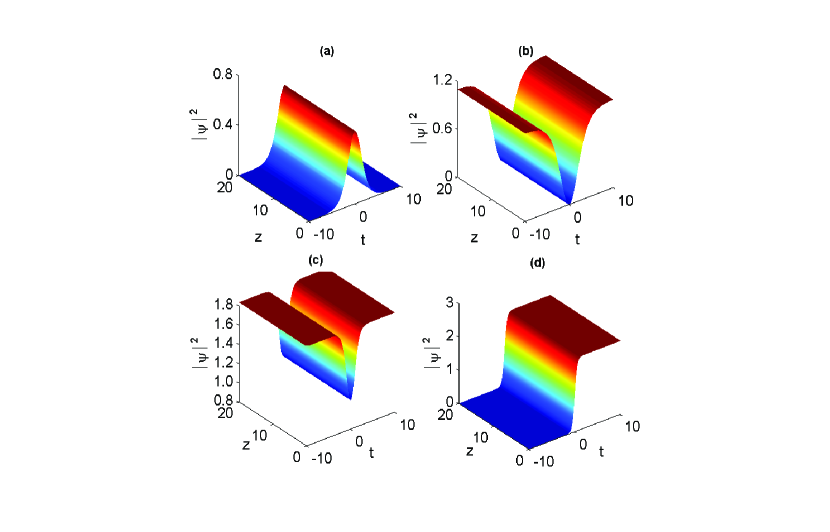
Figure 8: The numerical evolution of an initial (a) bright, (b) dark, (c) gray, and (d) kink pulses whose amplitude $10\%$ smaller than the exact solution. The parameters are the same as in Figs. 1(b), 3(b), 5(b), and 7(b) respectively.

We emphasize that the criterion in Eq. (80) does not depend on pseudo-quintic nonlinearity coefficient $\epsilon$ because this stability condition is the particular case of the general criterion in Eq. (79) when $I_{m}=0$. However, the general criterion in Eq. (79) depends on the parameter $\epsilon$ because the intensity $I(x)=u^{2}(x)$ of propagating waves and hence the parameter $I_{m}$ are the functions of coefficient $\epsilon$ in the case when $I_{m}\neq 0$.

Note that the stability criterion in Eq. (80) is equivalent to the condition $b>0$ where the parameter $b$ is introduced in Eq. (9). For an example, we have $I_{m}=0$ for the bright soliton given in Eq. (30), and hence the stability condition for this soliton solution is $b>0$. Thus the necessary conditions ($a<0$, $b>0$, and $3b^{2}>16ac$) for existence of this soliton are sufficient in appropriate experimental situation. We have also the parameter $I_{m}=0$ for the dark soliton solution in Eq. (39), and hence in this case the stability condition is $b>0$. However for the gray soliton solution in Eq. (52) we have two cases: (1) $I_{m}=A^{2}/(1+B)$ for $B>0$, and (2) $I_{m}=A^{2}$ for $-1<B<0$. Hence the stability condition for gray soliton in these two cases is given by Eq. (79) with appropriate values for parameter $I_{m}$. In the case of kink-type wave given in Eq. (61) we have $I_{m}=0$. Hence the conditions $a<0$ and $b>0$ with the constraint $3b^{2}/16ac=1$ are necessary and sufficient for existence of this kink-type waves in appropriate experimental situation. In the case of periodic waves presented in sec. III the stability criteria given in Eqs. (79) and (80) are also applicable.

V Numerical analysis

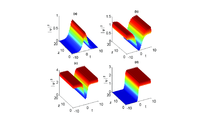
Figure 9: The numerical evolution of (a) the chirped bright solitary wave solution (30), (b) the chirped dark solitary wave solution (39), (c) the chirped gray solitary wave solution (52), and (d) the chirped kink solitary wave solution (61) under the perturbation of white noise whose maximal value is $0.1$. The parameters are the same as in Figs. 1(b), 3(b), 5(b), and 7(b) respectively.

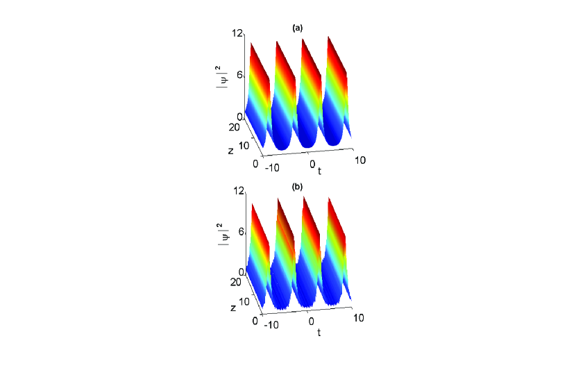
Figure 10: The numerical evolution of (a) the chirped periodic solution (33) with an initial wave amplitude $10\%$ smaller than the exact solution; (b) the chirped periodic solution (33) under perturbation of white noise whose maximal value is $0.1$. The parameters are the same as in Fig. 2.

In this section, we investigate the stability of the obtained periodic and solitary waves by using directly numerical simulations. It should be mentioned that only stable (or weakly unstable) solitary waves are promising for experimental observations and practical applications. Therefore, it is worthy to study the stability of these nonlinearly chirped structures with respect to finite perturbations. One notes that bright solitons are found to be stable in focusing Kerr-type media Aitchison . Moreover, important results have established the essential role played by higher-order nonlinearities in stabilizing the propagation of solitons. In this context, it was shown that the competition between focusing third-order and defocusing fifth-order nonlinearities supports stable soliton solutions Skarka . For our case of study, the generalized NLSE (1) involves such cubic-quintic nonlinearites, in addition to a derivative Kerr nonlinearity. It is therefore not unreasonable to conjecture that the obtained solutions are stable. However, a detailed analysis is required in order to strictly answer the stability problem of such privileged chirped nonlinear waveforms.

In order to analyze the stability of these chirped structures, we performed direct numerical simulations of Eq. (1) initialized with our computed solutions with added white noise and amplitude perturbation He ; R2 . We first perturb the amplitude ($10\%$) in the initial distribution. Figures 8(a)-8(d) show the evolution plots of chirped solitary-wave solutions (30), (39), (52), and (61) in which the amplitude in the initial distributions is perturbed. From these figures, one observes remarkably stable propagation of the localized solutions under the amplitude perturbation. Second, we add white noise ($10\%$) in the initial pulses. The numerical results are shown in Figs. 9(a)-9(d) in which the initial pulses are perturbed by white noise. Compared with Figs. 1(b), 3(b), 5(b), and 7(b), one can see that despite adding a white noise perturbation, the solutions remains intact after propagating a distance of twenty dispersion lengths. Thus, we can conclude that the obtained chirped bright, dark, gray, and kink solitary waves can propagate stably under the additive white noise perturbation. Next we study the evolution of the chirped periodic waves in the negative index material in the presence of small initial perturbations. Here we take the chirped periodic wave (33) as an example to analyze the stability of the solution numerically. We performed direct simulations with amplitude perturbation and initial white noise to study the stability of the solution (33) compared to Fig. 2(b). The numerical results are shown in Fig. 10(a) in which the initial amplitude is perturbed and Fig. 10(b) in which the solution is affected by the random noise. The results reveal that the finite initial perturbations of amplitude and additive white noise could not influence the main character of the periodic solutions. Therefore, the chirped solitary and periodic waves show structural stability with respect to the small input profile perturbations. Thus we conclude that the nonlinearly chirped structures we presented are stable in an appropriate range of parameters for soliton and periodic solutions of the generalized NLSE with pseudo-quintic nonlinearity and self-steepening effect.

VI Conclusion

In conclusion, we have demonstrated that several new fascinating types of periodic waves are formed in a NIM under the influence of pseudo-quintic nonlinearity and self-steepening effect. Such structures exhibit an interesting chirping property which shows a dependence on the light field intensity. Remarkably, the nonlinearity in pulse chirp is found to be caused by the presence of self-steepening process in the negative refractive index material. This is contrary to the case of vanishing self-steepening effect where only the unchirped envelope pulses are allowed to exist in the system in the presence of pseudo-quintic nonlinearity. Chirped periodic wave solutions expressed in terms of trigonometric functions have been also obtained for the governing generalized NLSE. These results constitute the first analytical demonstration of existence of periodic waves having a nonlinear chirp in negative-index media. Considering the long-wave limit of the derived periodic waves, we obtained a diversity of chirped localized solutions including bright, dark, kink, anti-kink, and gray solitary pulses. We further studied the stability of the nonlinearly chirped structures by using the theory of nonlinear dispersive waves and direct numerical simulations. Our results based on stability criterion and numerical simulations showed the robustness of those wave forms with respect to finite perturbations of the amplitude and additive white noise, thus motivating the experimental observations of such structures in materials which have negative index of refraction. Hence, we conclude that localized and periodic waves exhibiting a nonlinear chirp can be formed in negative refractive index media under the influence of pseudo-quintic nonlinearity and self-steepening effect. It is predicted in this paper that such chirped waves are experimentally realizable and hence these structures should be of relevance for applications requiring the use of a negative index material. One should note that the use of the above-mentioned generalized NLSE is not only restricted to ultrashort electromagnetic pulse propagation in negative refractive index media, but also to the description of light pulse dynamics in nonlinear fibers. Therefore the results presented in this work are also helpful for understanding the behavior of nonlinear waves in optical fiber systems. In the latter setting, the chirping property is of great advantage in fiber-optic applications such as the compression and amplification of light pulses and thus chirped pulses are particularly useful in the design of fiber-optic amplifiers, optical compressors, and solitary-wave-based communications links.

References

- (1) P. Li, R. Yang, and Z. Xu, Phys. Rev. E 82, 046603 (2010).
- (2) J. B. Pendry, Phys. Rev. Lett. 85, 3966 (2000).
- (3) E. J. Reed, M. Soljacic, and J. D. Joannopoulos, Phys. Rev. Lett. 91, 133901 (2003).
- (4) A. A. Zharov, I. V. Shadrivov, and Yu. S. Kivshar,Phys. Rev. Lett. 91, 037401 (2003).
- (5) C. G. Parazzoli, R. B. Greegor, K. Li, B. E. C. Koltenbah, and M. Tanielian, Phys. Rev. Lett. 90, 107401 (2003).
- (6) Y. Shen, P. G. Kevrekidis, G. P. Veldes, D. J. Frantzeskakis, D. DiMarzio, X. Lan, and V. Radisic, Phys. Rev. E 95, 032223 (2017).
- (7) Y. Xiang, X. Dai, S. Wen, J. Guo, and D. Fan, Phys. Rev. A 84, 033815 (2011).
- (8) G. Veselago, Sov. Phys. Usp. 10, 509 (1968).
- (9) J. B. Pendry, A. J. Holden, D. J. Robbins, and W. J. Stewart, IEEE Trans. Microwave Theory Tech. 47, 2075 (1999).
- (10) D. R. Smith and N. Kroll, Phys. Rev. Lett. 85, 2933 (2000).
- (11) D. R. Smith, W. J. Padilla, D. C. Vier, S. C. Nemat-Nasser, and S. Schultz, Phys. Rev. Lett. 84, 4184 (2000).
- (12) G. D’Aguanno, N. Mattiucci, M. Scalora, and M. J. Bloemer, Phys. Rev. Lett. 93, 213902 (2004).
- (13) A. K. Popov, V. V. Slabko, and V. M. Shalaev, Laser Phys. Lett. 3, 293 (2006).
- (14) S. C. Wen, Y. W. Wang, W. H. Su, Y. J. Xiang, X. Q. Fu, and D. Y. Fan, Phys. Rev. E 73, 036617 (2006); Y. J. Xiang, S. C. Wen, X. Y. Dai, Z. X. Tang, W. H. Su, and D. Y. Fan, J. Opt. Soc. Am. B 24, 3058 (2007).
- (15) P. P. Banerjee and G. Nehmetallah, J. Opt. Soc. Am. B 24, A69 (2007).
- (16) A. D. Boardman, P. Egan, L. Velasco, and N. King, J. Opt. A, Pure Appl. Opt. 7, S57 (2005); A. D. Boardman, R. C. Mitchell-Thomas, N. J. King, and Y. G. Rapoport, Opt. Commun. 283, 1585 (2010).
- (17) M. Scalora, M. S. Syrchin, N. Akozbek, E. Y. Poliakov, G. D’Aguanno, N. Mattiucci, M. J. Bloemer, and A. M. Zheltikov, Phys. Rev. Lett. 95, 013902 (2005).
- (18) S. Zhang and L. Yi, Phys. Rev. E 78, 026602 (2008).
- (19) M. Marklund, P. K. Shukla, and L. Stenflo, Phys. Rev. E 73, 037601 (2006).
- (20) R. Yang, X. Min, J. Tian, W. Xue and W. Zhang, Phys. Scr. 91, 025201 (2016).
- (21) S.H. Han, Q.H. Park, Phys. Rev. E 83, 066601 (2011).
- (22) A. Mahalingam and K. Porsezian, Phys. Rev. E 64, 046608 (2001).
- (23) W. J. Liu, L. H. Pang, H. N. Han, Z. W. Shen, M. Lei, H. Teng, and Z. Y. Wei, Photon. Res. 4, 111 (2016).
- (24) W.J. Liu, L. H. Pang, H.N. Han, K. Bi, M. Lei, and Z.Y. Wei, Nanoscale 9, 5806 (2017).
- (25) W.J. Liu, L. H. Pang, H.N. Han, M.L. Liu, M. Lei, S.B. Fang, H. Teng, Z.Y. Wei, Opt. Express 25, 2950 (2017).
- (26) W. J. Liu, Y.N. Zhu, Mengli Liu, B. Wen, S.B. Fang, H. Teng, M. Lei, L. M. Liu, Z. Y. Wei, Photonics Res. 6, 220 (2018).
- (27) Chenjian Wang, Zizhuo Nie, Weijie Xie, Jingyi Gao, Q. Zhou, W.J. Liu, Optik 184, 370 (2019).
- (28) W.J. Liu, Weitian Yu, Chunyu Yang, Mengli Liu, Yujia Zhang, Ming Lei, Nonlinear Dyn. 89, 2933 (2017).
- (29) Y.Y. Yan, W.J. Liu, Q. Zhou & A. Biswas Nonlinear Dyn. 99, 1313 (2020).
- (30) E. F. El-Shamy, Phys. Rev. E 91, 033105 (2015).
- (31) V. M. Petnikova and V. V. Shuvalov, Phys. Rev. E 76, 046611 (2007).
- (32) V. M. Petnikova and V. V. Shuvalov, Phys. Rev. E 79, 026605 (2009).
- (33) K. W. Chow and D. W. C. Lai, Phys. Rev. E 65, 026613 (2002).
- (34) C. Q. Dai, Y. Y. Wang, C. Yan, Opt. Commun. 283, 1489 (2010).
- (35) V. M. Petnikova, V. V. Shuvalov, V. A. Vysloukh, Phys. Rev. E 60, 1009 (1999).
- (36) V. I. Kruglov and H. Triki, Phys. Rev. A 103, 013521 (2021).
- (37) K. W. Chow, I. M. Merhasin, B. A. Malomed, K. Nakkeeran, K. Senthilnathan, and P. K. A. Wai, Phys. Rev. E 77, 026602 (2008).
- (38) K. W. Chow and C. Rogers, Phys. Lett. A 377, 2546 (2013).
- (39) F. Kh. Abdullaev, A. M. Kamchatnov, V. V. Konotop, and V. A. Brazhnyi, Phys. Rev. Lett. 90, 230402 (2003).
- (40) Z. Y. Yan, K.W. Chow, B. A. Malomed, Chaos, Solitons & Fractals 42,3013 (2009).
- (41) V. I. Kruglov, A. C. Peacock, and J. D. Harvey, Phys. Rev. E 71, 056619 (2005).
- (42) M. Desaix, L. Helczynski, D. Anderson, and M. Lisak, Phys. Rev. E 65, 056602 (2002).
- (43) X. Min, R. Yang, J. Tian, W. Xue, and J. M. Christian, J. Mod. Opt. 63, 44 (2016).
- (44) N. L. Tsitsas, T. P. Horikis, Y. Shen, P. G. Kevrekidis, N. Whitaker and D. J. Frantzeskakis, Phys. Lett. A 374, 1384 (2010).
- (45) S.C. Wen, Y.J. Xiang, X.Y. Dai, Z.X. Tang, W.H. Su, D.Y. Fan, Phys. Rev. A 75, 033815 (2007).
- (46) N. Tzoar and M. Jain, Phys. Rev. A 23, 1266 (1981).
- (47) D. Anderson and M. Lisak, Phys. Rev. A 27, 1393 (1983).
- (48) V. I. Kruglov and H. Triki, Phys. Rev. A 102, 043509 (2020).
- (49) H. Triki and V. I. Kruglov, Phys. Rev. E 101, 042220 (2020).
- (50) G. B. Whitham, J. Fluid Mech. 27, 399 (1967).
- (51) J. S. Aitchison, A. M. Weiner, Y. Silberberg, M. K. Oliver, J. L. Jackel, D. E. Leaird, E.M. Vogel, P. W. E. Smith, Opt. Lett. 15, 471 (1990).
- (52) V. Skarka, V.I. Berezhiani, R. Miklaszewski, Phys. Rev. E 56, 1080 (1997).
- (53) J.-d. He, J. Zhang, M. Y. Zhang, and C. Q. Dai, Opt. Commun. 285, 755 (2012).
- (54) R. Yang, L. Li, R. Hao, Z. Li, and G. Zhou, Phys. Rev. E 71, 036616 (2005).