A fundamental derivation of two Boris solvers and the Ge-Marsden theorem

Abstract

For a separable Hamiltonian, there are two fundamental, time-symmetric, second-order velocity-Verlet (VV) and position-Verlet (PV) symplectic integrators. Similarly, there are two VV and PV version of exact energy conserving algorithms for solving magnetic field trajectories. For a constant magnetic field, both algorithms can be further modified so that their trajectories are exactly on the gyro-circle. The magnetic PV integrator then becomes the well known Boris solver, while VV yields a second, previously unknown, Boris-type algorithm. Remarkably, the required on-orbit modification is a reparametrization of the time step, reminiscent of the Ge-Marsden theorem.

I Introduction

The Ge-Marsdenge88 theorem states that if a symplectic integrator (SI) exactly conserves the energy, but no other constants of motion, then its trajectory must be exact, up to “time-reparametrization”. The requirement that there are no other constants of motion except the energy seems to restrict its applicability to one-dimensional systems. The theorem is mainly used to argue that symplectic integrators cannot be exact energy conserving. From the modern perspective of deriving SI from Lie operators and Lie seriesdep69 ; dra76 ; yos93 ; chin20 , rather than from generating functionsfen10 , the theorem can be viewed as a corollary of approximating the exact evolution operator as a single product:

$${\rm e}^{{\Delta t}\hat{H}}={\rm e}^{{\Delta t}(\hat{T}+\hat{V})}\approx\prod_{i=1}^{N}{\rm e}^{a_{i}{\Delta t}\hat{T}}{\rm e}^{b_{i}{\Delta t}\hat{V}}={\rm e}^{{\Delta t}\hat{H}^{\prime}}$$ (1)

where for the standard separable Hamiltonian $H={\bf p}^{2}/2m+V({\bf r})$, $\hat{T}$ and $\hat{V}$ are Lie operators,

$$\hat{T}={\bf v}\cdot\frac{\partial}{\partial{\bf r}}\qquad{\rm and}\qquad\hat{V}={\bf a}({\bf r})\cdot\frac{\partial}{\partial{\bf v}}$$ (2)

with ${\bf v}\equiv{\bf p}/m$, ${\bf a}({\bf r})=-\nabla V/m$, and group actions

$${\rm e}^{{\Delta t}\hat{T}}({\bf r},{\bf v}) = ({\bf r}+{\Delta t}{\bf v},{\bf v})$$

$${\rm e}^{{\Delta t}\hat{V}}({\bf r},{\bf v}) = ({\bf r},{\bf v}+{\Delta t}{\bf a}).$$ (3)

The resulting modified Hamiltonian operator

$$\hat{H}^{\prime}=\hat{H}+{\Delta t}\hat{E}_{1}+{\Delta t}^{2}\hat{E}_{2}+{\Delta t}^{3}\hat{E}_{3}+\cdots$$ (4)

with various energy error terms $\hat{E}_{k}$, gives the trajectory of the algorithm via Hamilton’s equation with respect to the Hamiltonian functionyos93 $H^{\prime}$ corresponding to the operator $\hat{H}^{\prime}$. If for some reasons $\hat{H}^{\prime}=\hat{H}$ with all $\hat{E}_{k}=0$, then the trajectory produced by $H^{\prime}$ must be the same as the exact trajectory dictated by $H$. From this perspective, exact energy conservation implies exact trajectory is a general feature of symplectic integrators of the form (1), irrespective of whether there are other conserved quantities. This result only requires the existence of the modified Hamiltonian and its associated dynamics.

Moreover, the original proof of Gege88 allows for “time-reparametrization” of the formfen10 $H^{\prime}=F({\Delta t})H$, which usually does not occur in practice. This is because $H^{\prime}$ as given by (4) must have $F({\Delta t})=1$ due to the conventional requirements

$$\sum_{i=1}^{N}a_{i}=1\quad{\rm and}\quad\sum_{i=1}^{N}b_{i}=1.$$ (5)

This can be easily verified by applying the following second-order velocity-Verlet (VV) SI

$${\bf v}_{1} = {\bf v}_{0}+\frac{1}{2}{\Delta t}{\bf a}({\bf r}_{0})$$ (6)

$${\bf r}_{1} = {\bf r}_{0}+{\Delta t}{\bf v}_{1}$$ (7)

$${\bf v}_{2} = {\bf v}_{1}+\frac{1}{2}{\Delta t}{\bf a}({\bf r}_{1})$$ (8)

corresponding to $N=2,a_{1}=0,b_{1}=1/2,a_{2}=1,b_{2}=1/2$ in (1), and the position-Verlet (PV) SI

$${\bf r}_{1} = {\bf r}_{0}+\frac{1}{2}{\Delta t}{\bf v}_{0}$$

$${\bf v}_{1} = {\bf v}_{0}+{\Delta t}{\bf a}({\bf r}_{1})$$ (9)

$${\bf r}_{2} = {\bf r}_{1}+\frac{1}{2}{\Delta t}{\bf v}_{1}.$$ (10)

corresponding to $N=2,a_{1}=1/2,b_{1}=1,a_{2}=1/2,b_{2}=0$ in (1), to the case of a constant force with ${\bf a}({\bf r})={\bf a}$. Both algorithms then give the final position (7) and (10) as ${\bf r}_{1,2}({\Delta t})={\bf r}_{0}+{\Delta t}{\bf v}_{0}+\frac{1}{2}{\Delta t}^{2}{\bf a}$, which is the exact trajectory for all ${\Delta t}$ with no time-reparametrization. The author is unaware of any example of the Ge-Marsden theorem with manifest time-reparametrization. It is therefore a complete surprise, that a highly non-trivial time-reparametrization is needed to obtain exact trajectories in a constant magnetic field. A resulting algorithm from such a time-reparametrization is none other than the well known Boris solver of plasma physics.

The Boris solverbun67 ; bor70 ; bir85 has been widely regarded as the gold standard for solving charged particle trajectories in plasmabir85 and astrophysicsrip18 . But why is it so goodqin13 ? Recent works focusing on volume-preserving methodsqin13 ; he15 do not explain why the Boris solver is unique among all volume preserving algorithms. The real reason why the Boris solver is so good, according to Bunemanbun67 , who proposed an earlier version of the solver, is that “it leads to points on exact cycloids whenever E and B are constant”. That is, for a constant magnetic field, positions generated by the Buneman solverbun67 are exactly on the gyro-circle, the cyclotron orbit. However, when Buneman’s original ${\bf E}\times{\bf B}$ formulation was abandonbir85 in favor of Boris’s ${\bf E}$, ${\bf B}$ splitting scheme, this point seems to have been forgotten, especially when only the first-order leap-frog version of the Boris solver is usedbir85 ; par91 ; vu95 ; comm . Otherwise, this on-orbit property need not be pointed out again by otherssto02 when using the second-order solvercomm .

The same operator method used to derive symplectic integrator above has been used by the author to derive exact energy conserving (EEC) integrators for solving charged particle trajectories in a general magnetic fieldchin08 . Since these algorithms use the Lorentz force law directly in terms of the mechanical momentum rather than the canonical momentum, these algorithms are EEC but not symplectic. (They are referred to as Poisson integrators in Ref.kna15, .) Because of this, their properties are not directly related to the Ge-Marsden theorem: they conserved the energy exactly, yet their trajectories are not exact. For a constant magnetic field, their orbits are not on the gyro-circle. According to Bunemanbun67 , that can only be achieved with additional “cycloid fitting”. Remarkably, this work shows that this “cycloid fitting” can be done exactly by a time-step reparametrization, a possibility suggested by the Ge-Marsden theorem. One of the resulting algorithm is then the Boris solver.

This work presents a completely original derivation of Boris solvers independent of any finite-difference schemes, including a previously unknown second Boris solver. To see how these two Boris solvers are related to symplectic integrators, this work will review in the next section, the magnetic velocity-Verlet and position-Verlet integrators previously derived in Ref.chin08, . In Sect.III, the two Boris solvers are derived by “cycloid fitting”. Simple higher order algorithms are then constructed in Sect.IV. Conclusions are stated in Sect.V.

II The two fundamental magnetic algorithms

For a charged particle $q$ in a magnetic field ${\bf B({\bf r})}=B({\bf r})\hat{\bf B}({\bf r})$, its acceleration is given by the Lorentz force law:

$$\frac{d{\bf v}}{dt}=\omega({\bf r})\hat{\bf B}({\bf r})\times{\bf v},$$ (11)

where $\omega({\bf r})=(-q)B({\bf r})/m$ is the local cyclotron angular frequency. (Note that $\omega$ is correctly positive for $q<0$ because if $\hat{\bf B}({\bf r})$ is out of the page, the cyclotron motion is counterclockwise.) The operator $\hat{V}$ in (2) is then replaced by

$$\hat{V}_{B}=\omega(\hat{\bf B}\times{\bf v})\cdot\frac{\partial}{\partial{\bf v}},$$ (12)

whose effect on ${\bf v}$ is just

$$\hat{V}_{B}{\bf v} = (\omega\hat{\bf B}\times){\bf v}$$

$$\hat{V}_{B}^{n}{\bf v} = (\omega\hat{\bf B}\times)^{n}{\bf v}$$ (13)

and therefore the velocity update is

$${\bf v}_{B}({\bf r},{\bf v},{\Delta t}) = {\rm e}^{{\Delta t}\hat{V}_{B}}{\bf v}={\rm e}^{\theta(\hat{\bf B}\times\ )}{\bf v}$$ (14)

$$= {\bf v}+({\theta}-\frac{{\theta}^{3}}{3!}+\frac{{\theta}^{5}}{5!}+\cdots)\hat{\bf B}\times{\bf v}+(\frac{{\theta}^{2}}{2}-\frac{{\theta}^{4}}{4!}+\cdots)\hat{\bf B}\times(\hat{\bf B}\times{\bf v})$$ (15)

$$= {\bf v}+\sin{\theta}\hat{\bf B}\times{\bf v}+(1-\cos{\theta})\hat{\bf B}\times(\hat{\bf B}\times{\bf v})$$ (16)

where $\theta=\omega({\bf r}){\Delta t}$ and where one has repeatedly used the identity

$$\hat{\bf B}\times(\hat{\bf B}\times(\hat{\bf B}\times{\bf v}))=-\hat{\bf B}\times{\bf v}$$ (17)

to reduce the exponential series to (15) and resummed as (16), which is the exact solution to (11) holding ${\bf r}$ fixed. By decomposing ${\bf v}$ into components parallel and perpendicular to $\hat{\bf B}({\bf r})$

$${\bf v}={\bf v}_{||}+{\bf v}_{\perp},$$ (18)

so that $\hat{\bf B}\times(\hat{\bf B}\times{\bf v}_{\perp})=-{\bf v}_{\perp}$, (16) becomes

$${\bf v}_{B}({\bf r},{\bf v},{\Delta t})={\bf v}_{||}+\cos{\theta}{\bf v}_{\perp}+\sin{\theta}(\hat{\bf B}\times{\bf v}_{\perp}).$$ (19)

This shows that the magnetic field only rotates the perpendicular velocity component without changing the velocity’s magnitude and hence the kinetic energy.

By replacing the velocity updates in (6), (8) and (9) by (16), or (19), one obtains the corresponding magnetic integrator M2a

$${\bf v}_{1} = {\bf v}_{B}({\bf r}_{0},{\bf v}_{0},{\Delta t}/2)$$ (20)

$${\bf r}_{1} = {\bf r}_{0}+{\Delta t}{\bf v}_{1}$$ (21)

$${\bf v}_{2} = {\bf v}_{B}({\bf r}_{1},{\bf v}_{1},{\Delta t}/2)$$ (22)

and M2b

$${\bf r}_{1} = {\bf r}_{0}+\frac{1}{2}{\Delta t}{\bf v}_{0}$$

$${\bf v}_{1} = {\bf v}_{B}({\bf r}_{1},{\bf v}_{0},{\Delta t})$$ (23)

$${\bf r}_{2} = {\bf r}_{1}+\frac{1}{2}{\Delta t}{\bf v}_{1}$$ (24)

as derived in Ref.chin08, . Each is completely explicit, sequential, exact energy conserving, but not symplectic. This is because in order to be symplectic, one must update the canonical momentum in Hamilton’s equations of motion. Since the Lorentz force law (11) uses only the mechanical momentum, any direct use of the Lorentz force law is non-canonical and therefore non-symplectic.

To see how these magnetic integrators work, consider the case of an electron in a constant magnetic field with $\omega=2$, $\hat{\bf B}=\hat{\bf z}$, ${\bf r}=(x,y)$, ${\bf v}={\bf v}_{\perp}=(v_{x},v_{y})$, with initial velocity ${\bf v}_{0}=(0,v_{0})$, ${\bf r}_{0}=(r_{g},0)$, where $v_{0}=1$ and where $r_{g}=v_{0}/\omega=1/2$ is the gyro-radius. Let’s take a large ${\Delta t}=\pi/4$, so that ${\theta}=\omega{\Delta t}=\pi/2$. Therefore both ${\bf r}$ and ${\bf v}$ rotate through $90^{\circ}$ 4 times to complete one orbit. The M2a and M2b trajectories are the square orbits shown in Fig.1. For M2a, the position update (21) is ${\Delta t}$ times the initial velocity rotated $45^{\circ}$, so the length of the displacement is $v_{0}{\Delta t}$. For M2b, the position update (24) is ${\Delta t}$ times half the diagonal of a square with sides $v_{0}$, which is $v_{0}{\Delta t}/\sqrt{2}$. Therefore the displacement of M2a is $\sqrt{2}$ times that of M2b, as shown. Their trajectories fall outside and inside of the gyro-circle respectively.

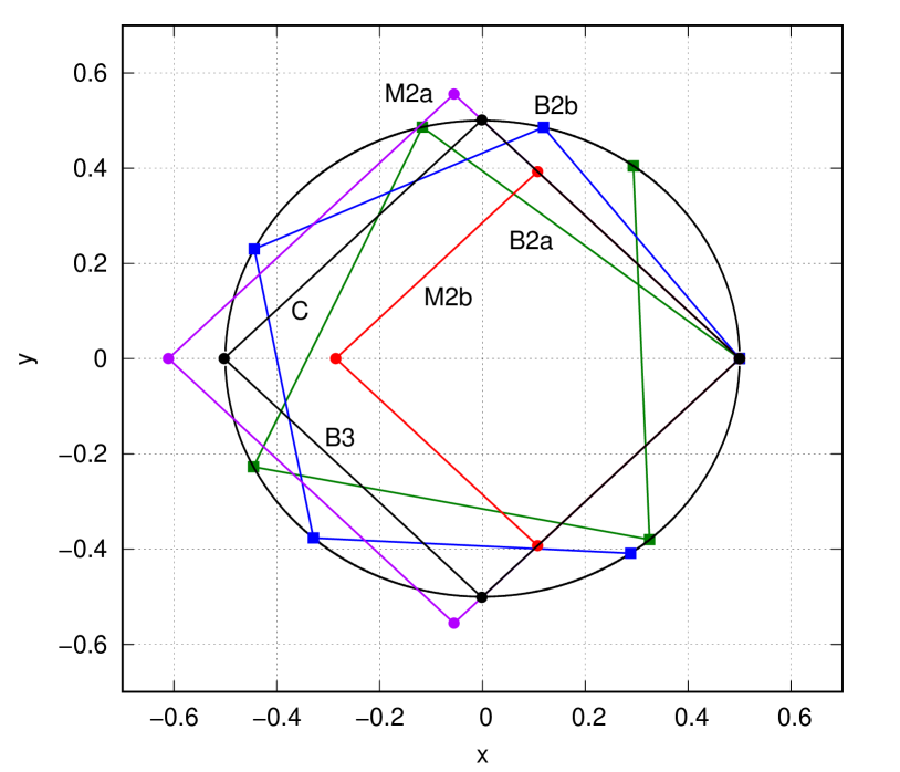
Figure 1: (color online) All orbits start on the rightmost point on the gyro-circle. M2a and M2b have three points outside and inside of the circle respectively. B2b and B2a have points on the circle but with angles behind and ahead of the phase correct angle of M2a and M2b. C and B3 are higher order results having very small error off the circle and very small phase error respectively. See text for details.

III cycloid fitting

For M2b, the position updating step (24) is

$${\bf r}_{2} = {\bf r}_{0}+\frac{1}{2}{\Delta t}({\bf v}_{0}+{\bf v}_{1})$$ (25)

$$= {\bf r}_{0}+\frac{1}{2}{\Delta t}({\bf v}_{0}+\cos{\theta}{\bf v}_{0}+\sin{\theta}\hat{\bf B}\times{\bf v}_{0})$$

Defining ${\bf r}_{g}={\bf v}_{0}/\omega=(0,r_{g})$ and noting that ${\bf r}_{0}=(r_{g},0)=-\hat{\bf B}\times{\bf r}_{g}$, one can rewrite the above as

$${\bf r}_{2} = \frac{{\theta}}{2}(1+\cos{\theta}){\bf r}_{g}-(1-\frac{{\theta}}{2}\sin{\theta})\hat{\bf B}\times{\bf r}_{g}),$$ (26)

and therefore the trajectory is always inside of the gyro-circle:

$$|{\bf r}_{2}|^{2} = r_{g}^{2}\left[1-2{\theta}\cos^{2}(\frac{{\theta}}{2})\Bigl{(}\tan(\frac{{\theta}}{2})-\frac{{\theta}}{2}\Bigr{)}\right]$$ (27)

$$= r_{g}^{2}[1-\frac{1}{12}{\theta}^{4}+\frac{1}{80}{\theta}^{6}+\cdots]\ {\rm as}\ {\theta}\rightarrow 0.$$ (28)

However, if one were to decouple the actual rotation angle (arguments of trig functions) from ${\theta}$ to an effective angle ${\theta}_{B}$, then requiring

$$\tan(\frac{{\theta}_{B}}{2})=\frac{{\theta}}{2}$$ (29)

in (27) would force the trajectory to be exactly on the gyro-circle! This corresponds to a highly non-trivial reparametrization of ${\Delta t}$ in the rotation angle to a Boris time step ${\Delta t}_{B}$ via

$${\Delta t}_{B}=\frac{2}{\omega}\tan^{-1}(\omega{\Delta t}/2).$$ (30)

If the updating rotation step (19) is replaced by

$${\bf v}_{B}({\bf r},{\bf v},{\Delta t})={\bf v}_{||}+\cos{\theta}_{B}{\bf v}_{\perp}+\sin{\theta}_{B}(\hat{\bf B}\times{\bf v}_{\perp}),$$ (31)

then M2b reproduces the Boris solver denoted here as B2b. From (29), $\cos{\theta}_{B}$ and $\sin{\theta}_{B}$ can be easily reconstructed as

$$\sin{\theta}_{B} = \frac{2\tan({\theta}_{B}/2)}{1+\tan^{2}({\theta}_{B}/2)}=\frac{{\theta}}{1+{\theta}^{2}/4},$$ (32)

$$\cos{\theta}_{B} = \frac{1-\tan^{2}({\theta}_{B}/2)}{1+\tan^{2}({\theta}_{B}/2)}=\frac{1-{\theta}^{2}/4}{1+{\theta}^{2}/4}.$$ (33)

This makes it clear that the position vector (26)

$${\bf r}_{2} = \frac{{\theta}}{1+\frac{1}{4}{\theta}^{2}}{\bf r}_{g}-\frac{1-\frac{1}{4}{\theta}^{2}}{1+\frac{1}{4}{\theta}^{2}}\hat{\bf B}\times{\bf r}_{g}$$

$$= \sin({\theta}_{B}){\bf r}_{g}-\cos({\theta}_{B})\hat{\bf B}\times{\bf r}_{g}$$

$$= \cos({\theta}_{B}-\pi/2){\bf r}_{g}+\sin({\theta}_{B}-\pi/2)\hat{\bf B}\times{\bf r}_{g},$$ (35)

is not only precisely on the gyro-circle, but it lags $90^{\circ}$ behind, and is therefore perpendicular to the Boris-angle rotated velocity vector (31).

The resulting trajectory in Fig.1 is labeled as B2b. Notice that B2b’s angle of rotation lags behind that of the M2a and M2b. This follows from ${\theta}=\pi/2=1.5708$,

$${\theta}_{B}=2\tan^{-1}({\theta}/2)=1.3316\quad{\rm and}\quad{\theta}_{B}-{\theta}=-0.2392\ .$$ (36)

More generally at small ${\theta}$, the Boris angle ${\theta}_{B}$ has a second order phase error,

$${\theta}_{B}={\theta}[1-\frac{1}{12}{\theta}^{2}+\frac{1}{80}{\theta}^{4}+\cdots],$$ (37)

showing B2b’s rotation angle always lags, but remarkably with the same two leading coefficients as in gyro-radius (28). For extensive comparisons of B2b with M2a and M2b on nonuniform magnetic fields, see the work by Knapp, Kendl, Koskela and Ostermannkna15 .

Since ${\theta}_{B}$ can be defined via (29) for all ${\Delta t}$, B2b’s trajectory will stay on the gyro-circle for all ${\Delta t}$, no matter how large. In the limit of ${\theta}\rightarrow\infty$, ${\theta}_{B}\rightarrow\pi$, B2b’s trajectory will just bounce back and forth nearly as straight lines across the diameter of the gyro-circle. Nevertheless, this means that B2b’s trajectory remains bounded even as ${\Delta t}\rightarrow\infty$! It is unusual that an explicit algorithm can be unconditionally stable.

Conventionally, the stability of the original Boris solver was thought to be connected to the Cayley approximation for the exponential operator in (14):

$${\rm e}^{\theta(\hat{\bf B}\times\ )}\approx[1-\frac{1}{2}\theta(\hat{\bf B}\times\ )]^{-1}[1+\frac{1}{2}\theta(\hat{\bf B}\times\ )]\equiv{\bf C},$$ (38)

found in the implicit midpoint approximation used in Boris’s original derivationbor70 . By expanding the inverse operator as $1/(1-x)=1+x+x^{2}+\cdots$ and recollecting terms as in (15), one finds the same Boris rotation:

$${\bf C}{\bf v} = [1+\frac{\frac{1}{2}{\theta}(\hat{\bf B}\times\ )+\frac{1}{4}{\theta}^{2}(\hat{\bf B}\times\ )^{2}}{1+\frac{1}{4}{\theta}^{2}}][1+\frac{1}{2}{\theta}(\hat{\bf B}\times\ )]{\bf v},$$ (39)

$$= [1+\frac{{\theta}(\hat{\bf B}\times\ )+\frac{1}{2}{\theta}^{2}(\hat{\bf B}\times\ )^{2}}{1+\frac{1}{4}{\theta}^{2}}]{\bf v},$$

$$= {\bf v}_{||}+\frac{1-\frac{1}{4}{\theta}^{2}}{1+\frac{1}{4}{\theta}^{2}}{\bf v}_{\perp}+\frac{{\theta}}{1+\frac{1}{4}{\theta}^{2}}(\hat{\bf B}\times{\bf v}_{\perp}).$$

However, by itself, this Boris rotation (39), no more than the exact rotation (19), can confer greater stability. That is, if this Boris rotation (39) is just another mathematical means of rotating the velocity vector (but without evaluating trigonometric functions), then there is no a prior reason to expect that it would work better than the exact rotation (19). However, this derivation showed that the Boris angle condition (29) forces the trajectory to be on the gyro-circle. It is by enforcing this physical property that the Boris rotation can achieve greater, and in this case, unconditional stability. In principle, the angle condition (29) is totally sufficient to define the Boris rotation (31) via (32) and (33). It is entirely irrelevant whether this angle condition can be realized by any specific approximation of the exponential operator such as the Cayley transform (38).

For M2a, the position updating step (21) is

$${\bf r}_{1} = {\bf r}_{0}+{\Delta t}[\cos({\theta}/2){\bf v}_{0}+\sin({\theta}/2)\hat{\bf B}\times{\bf v}_{0}]$$ (40)

$$= {\theta}\cos({\theta}/2){\bf r}_{g}+({\theta}\sin({\theta}/2)-1)\hat{\bf B}\times{\bf r}_{g})$$ (41)

$$|{\bf r}_{1}|^{2} = r_{g}^{2}\left[1+2{\theta}\left(\frac{{\theta}}{2}-\sin(\frac{{\theta}}{2})\right)\right]$$ (42)

$$= r_{g}^{2}[1+\frac{1}{24}{\theta}^{4}-\frac{1}{1920}{\theta}^{6}+\cdots]\ {\rm as}\ {\theta}\rightarrow 0.$$

Therefore, if one now defines a second Boris angle ${\theta}^{\prime}_{B}$ by

$$\sin(\frac{{\theta}^{\prime}_{B}}{2})=\frac{{\theta}}{2},$$ (43)

and set

$$\cos(\frac{{\theta}^{\prime}_{B}}{2})=\sqrt{1-(\frac{{\theta}}{2})^{2}}$$ (44)

in (20) and (22), then one obtains a second, previously unknown, Boris solver whose trajectory is also exactly on the gyro-circle. The position vector (41) is then

$${\bf r}_{1} = {\theta}\sqrt{1-(\frac{{\theta}}{2})^{2}}\ {\bf r}_{g}-(1-{\theta}^{2}/2)\hat{\bf B}\times{\bf r}_{g})$$

$$= \sin({\theta}^{\prime}_{B}){\bf r}_{g}-\cos({\theta}^{\prime}_{B})\hat{\bf B}\times{\bf r}_{g}$$

$$= \cos({\theta}^{\prime}_{B}-\pi/2){\bf r}_{g}+\sin({\theta}^{\prime}_{B}-\pi/2)\hat{\bf B}\times{\bf r}_{g},$$ (46)

which is again $90^{\circ}$ behind the ${\theta}^{\prime}_{B}$ rotated velocity.

This second Boris solver’s orbit is labeled as B2a in Fig.1. Here, ${\theta}^{\prime}_{B}$ is ahead of M2a and M2b by an amount nearly equal to that of (36):

$${\theta}^{\prime}_{B}=2\sin^{-1}({\theta}/2)=1.8067\quad{\rm and}\quad{\theta}^{\prime}_{B}-{\theta}=0.2359\ .$$ (47)

At small ${\theta}$, ${\theta}^{\prime}_{B}$ remains ahead, with second-order error

$${\theta}^{\prime}_{B}={\theta}[1+\frac{1}{24}{\theta}^{2}+\frac{3}{640}{\theta}^{4}+\cdots]$$ (48)

having the same leading coefficient as in (42), but not the exact opposite of (37).

From (43), this ${\theta}^{\prime}_{B}$ can only be defined for $|{\theta}/2|\leq 1$. Therefore this second Boris solver is limited to $|{\Delta t}|<|2/\omega|=T/\pi$, approximately a third of the gyro-period. This same range of stability is obtained when the symplectic VV integrator is applied to the harmonic oscillatorchin20 .

This second Boris solver also underscores the fact it is the second Boris angle condition (43) that is of paramount importance. The use of the Cayley transform (38) here would not have improved the M2a integrator in any way. Also, it is not clear whether this second Boris condition (43) can be realized by a Cayley-like operator approximation of the exponential, as in (38).

Finally, note that for motion perpendicular to $\hat{\bf B}$, since

$$\frac{d}{dt}({\bf r}^{2})=2{\bf r}\cdot{\bf v}\quad{\rm and}\quad\frac{d({\bf r}\times{\bf v})}{dt}=\omega({\bf r}\cdot{\bf v})\hat{\bf B},$$ (49)

the constancy of $r^{2}$, the orthogonality of ${\bf v}$ to ${\bf r}$, and the conservation of angular momentum, are one and the same condition.

IV Higher order algorithms

Given basic second-order algorithms M2a, M2b and B2b, B2a, well known methodschin08 ; he15 ; kna15 can be used to generate higher order schemes. However, some schemes are so simple that they can be constructed by inspection. For example, in view of (28) and (42), the combination algorithm

$$C({\Delta t})=\frac{2}{3}M2a({\Delta t})+\frac{1}{3}M2b({\Delta t}),$$ (50)

would have sixth-order $r_{g}^{2}$ error at small ${\Delta t}$:

$$|{\bf r}|^{2}=r_{g}^{2}[1+\frac{11}{2880}{\theta}^{6}+\cdots].$$ (51)

Surprisingly, it is already very good even at ${\Delta t}=\pi/4$. This is shown as the square orbit $C$ in Fig.1. As pointed out previously, the length of the M2a step is $v_{0}{\Delta t}=\pi/4$, the length of the M2b step is $(\pi/4)/\sqrt{2}$. The length of the combination C step is therefore

$$\frac{2}{3}\frac{\pi}{4}+\frac{1}{3}\frac{\pi}{4}\frac{1}{\sqrt{2}}=\frac{\pi}{12}(2\sqrt{2}+1)\frac{1}{\sqrt{2}}\approx 1.002\frac{1}{\sqrt{2}}$$ (52)

Since the length require to be on the gyro-circle is $1/\sqrt{2}$, algorithm C’s slight over-shoot is not visually visible. Since C has no phase error, it is very close to, but not exactly on the gyro-circle.

For B2b and B2a, since their trajectories are already on the gyro-circle, one can only improve their phase error. To preserve their positions on the gyro-circle, one must apply B2b and B2a sequentially. In view of (37) and (48), a time-symmetric sequence is

$$B3({\Delta t})=B2a(\frac{{\Delta t}}{3})B2b(\frac{{\Delta t}}{3})B2a(\frac{{\Delta t}}{3})$$ (53)

with Boris angle

$${\theta}_{B3} = 4\sin^{-1}({\theta}/6)+2\tan^{-1}({\theta}/6)$$ (54)

$$\qquad={\theta}[1+\frac{7}{77760}{\theta}^{4}\cdots].$$

For the case considered, ${\theta}=\pi/2$,

$${\theta}_{B3}=1.0005(\frac{\pi}{2}),$$

which is, surprisingly, already in agreement with the small angle estimate (54). The resulting orbit, labeled B3, overlaps with orbit C in Fig.1.

V Conclusions and future directions

In this work, two Boris solvers are derived from two fundamental magnetic field integrators M2b and M2a. This derivation demonstrated the underlying unity among all second-order explicit algorithms, from symplectic, magnetic to Boris integrators. There is no need to tinker with various finite-difference schemes or concoct ad hoc adjustments. There are only two fundamental algorithms in all cases, from which higher order schemes can be systematically constructed.

As shown in the Introduction, a constant force, including that from a constant electric field, can be exactly integrated by a second-order algorithm. Therefore, for a constant electric and magnetic field, cycloid fitting, as shown by Buneman solverbun67 , remains just fitting the gyro-circle. The added electric field can be easily accounted for by splittingbor70 ; kna15 .

Boris originally suggestedbor70 ; sto02 the $\tan(\alpha)/\alpha$ modification, which is to replace ${\theta}/2$ by $\tan({\theta}/2)$, so that his solver’s phase would be correct by retracing (32) and (33) in the reverse order. However, this work showed that such a modification would simply revert B2b back to M2b, losing large ${\Delta t}$ stability and going off the gyro-circle.

From (3), the characteristics of symplectic integrators are position and velocity translations. From (19), the characteristics of magnetic integrators are position translations and velocity rotations. They are therefore fundamentally different. For symplectic integrators, the Ge-Marsden theorem correctly single out the algorithm’s energy, the modified Hamiltonian, as the controlling factor in determining the trajectory’s accuracy. For purely magnetic integrators, because they are not Hamiltonian based, the controlling factor is not known. It is not clear what plays the role equivalent to the modified Hamiltonian. This work showed that exact energy conserving magnetic integrators must have reparametrized time steps, or phase errors, in order to produce exact trajectories. Yet, the derivation is just retrofitting, one has no theory of how to exploit the phase freedom to achieve greater trajectory accuracy. All these suggest that an equivalent Ge-Marsden theorem for magnetic integrators would be most helpful in guiding the future development of more efficient magnetic algorithms.

References

- (1) Ge Zhong and J. Marsden,“Lie-Poisson Hamilton-Jacobi Theory and Lie-Poisson Integrators”, Phys. Lett. A 133, 134 (1988).
- (2) A. Deprit “Canonical transformations depending on a small parameter” Celest. Mech. Dyn. Astron. 1, 12-39 (1969).
- (3) A. J. Dragt and J. M. Finn, “Lie series and invariant functions for analytic symplectic maps”, J. Math. Phys. 17, 2215-2224 (1976).
- (4) H. Yoshida, “ Recent progress in the theory and application of symplectic integrators”, Celest. Mech. Dyn. Astron. 56, 27-43 (1993).
- (5) S. A. Chin, “Structure of numerical algorithms and advanced mechanics”, Am. J. Phys. 88, 883 (2020); doi: 10.1119/10.0001616
- (6) Kang Feng and Mengzhao Qin, Symplectic geometric algorithms for Hamiltonian systems, Springer, Berlin, 2010.
- (7) O. Buneman, “Time-Reversible Difference Procedure”, J. Comput. Phys. 1, 517 (1967).
- (8) J. Boris, in Proceedings of the Fourth Conference on Numerical Simulation of Plasmas, (Naval Research Laboratory, Washington DC, 1970), p. 3.
- (9) C. Birdsall and A. Langdon, Plasma Physics Via Computer Simulation (McGraw-Hill, Inc., New York, 1985), p. 356.
- (10) B. Ripperda , F. Bacchini , J. Teunissen , C. Xia , O. Porth , L. Sironi , G. Lapenta , and R. Keppens “A Comprehensive Comparison of Relativistic Particle Integrators”, Astrophys. J. Suppl. Series, 235:21, (2018), https://doi.org/10.3847/1538-4365/aab114.
- (11) H. Qin, S. X. Zhang, J. Y. Xiao, J. Liu, Y. J. Sun, and W. M. Tang, “Why is Boris algorithm so good?” Phys. Plasmas 20, 084503 (2013).
- (12) Y. He, Y. J. Sun, J. Liu, and H. Qin, “Volume-preserving algorithms for charged particle dynamics,” J. Comput. Phys. 281, 135 (2015)
- (13) S.E. Parker and C.K. Birdsall, “Numerical error in electron orbits with large ”, J. Comput. Phys. 97 (1991) 91–102.
- (14) H.X. Vu, J.U. Brackbill, “Accurate numerical solution of charged particle motion in a magnetic field”, J. Comput. Phys. 116(2) (1995) 384–387.
- (15) The confusion and distinction between the first and second-order Boris solvers will be clarified in a forthcoming article.
- (16) P. H. Stoltz, J. R. Cary, G. Penn, and J. Wurtele, “Efficiency of a Boris like integration scheme with spatial stepping,” Phys. Rev. Spec. Top. Accel. Beams 5, 094001 (2002).
- (17) S. A. Chin, “Symplectic and energy-conserving algorithms for solving magnetic field trajectories”, Phys. Rev. E 77, 066401 (2008).
- (18) Christian Knapp, Alexander Kendl, Antti Koskela, and Alexander Ostermann “Splitting methods for time integration of trajectories in combined electric and magnetic fields” Phys. Rev. E 92, 063310 (2015)