De Sitter Holography:

Fluctuations, Anomalous Symmetry, and Wormholes

Leonard Susskind

Stanford Institute for Theoretical Physics and Department of Physics,

Stanford University, Stanford, CA 94305-4060, USA

and

Google, Mountain View, CA

The Goheer-Kleban-Susskind no-go theorem says that the symmetry of de Sitter space is incompatible with finite entropy. The meaning and consequences of the theorem are discussed in the light of recent developments in holography and gravitational path integrals. The relation between the GKS theorem, Boltzmann fluctuations, wormholes, and exponentially suppressed non-perturbative phenomena suggests: the classical symmetry between different static patches is broken; and that eternal de Sitter space—if it exists at all—is an ensemble average.

1 Introduction

All phenomena in a region of space can be described by a set of degrees of freedom localized on the boundary of that region, with no more than one degree of freedom per Planck area.

The Holographic Principle has been the driving force behind many of the advances in quantum gravity over the last twenty five years, but up to now the only precise examples have been cosmologies, which like anti de Sitter space, have asymptotically cold time-like causal boundaries. The reliance on the existence of such boundaries is troubling because the space we live in seems not to have one. Instead it has a horizon and a space-like warm boundary. If the HP is to apply to the real world then we need to generalize it.

So, does the Holographic Principle apply to cosmologies like de Sitter space? If yes, then what are the rules? I don’t know for sure, and this paper will not conclusively answer the question, but I will try to lay out some tentative principles.

Two things that will not be found here are specific models and applications to phenomenology.

1.1 An Obstruction? Or Not

Some time ago Goheer, Kleban, and I (GKS) [1] proved a theorem that it is impossible for a quantum system to satisfy the symmetries of classical de Sitter space if the entropy is finite. At the time, I interpreted this as a no-go theorem for absolutely stable (eternal) de Sitter space, but recent developments in quantum gravity suggest that a different interpretation might be possible. The idea is that a de Sitter vacuum might be eternal but the symmetries only approximate, being violated by exponentially small non-perturbative effects. The mechanisms are very similar to ones that have recently been uncovered in the SYK system and its gravitational dual.

1.2 Eternal de Sitter Space

By eternal de Sitter space  I mean a cosmology that is trapped in a state of finite entropy and cannot escape through reheating or tunneling to a larger “terminal vacuum” [2][3][4][5][6]. Eternal de Sitter space  might arise from a landscape in which the scalar fields have strictly positive potential, greater than some finite positive gap, in which there is one or more minima of $V.$ Figure 1 illustrates this kind of potential. I don’t know if a landscape with these properties can exist in a real theory of quantum gravity but let’s assume that it can, and see where it takes us.

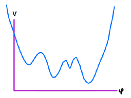
Figure 1: A schematic landscape for eternally stable de Sitter space. The universe spends most of its time in the lowest minimum with rare fluctuations to higher points.

Classically the different minima lead to different stable de Sitter geometries, but in quantum mechanics tunneling allows transitions between the minima. This leads to a single thermal equilibrium state (of a static patch) which mostly sits in the lowest minimum. But occasional Boltzmann fluctuations allow transitions to higher minima, followed by tunneling back to the lowest minimum. The rates for such fluctuations are of order $\exp{(-S_{0})}$ where $S_{0}$ is the nominal entropy of the de Sitter space at the lowest minimium. Other less extreme fluctuations can take place; for example the horizon of a static patch may spontaneously emit an object such as a black hole. These freak fluctuations are the only things that happen in the closed quantum world of a de Sitter static patch [7][8], but thermal correlations contain a wealth of information about non-equilibrium dynamics.

Eternal de Sitter space  is of course eternal, both to the future and to the past. Among the possible Boltzmann fluctuations that can take place over an enormous expanse of time are transitions to what we ordinarily think of as the initial conditions of our universe. I have in mind a fluctuation to to an inflationary point on the landscape, which after some inflation eventually evolves to a standard $\Lambda$-CDM universe. That of course would not be the end of the story. After a very long period of $\Lambda$-dominance a fluctuation will occur to another minimum and the whole process will repeat.

While this may be possible, a theory based on Boltzmann fluctuations is a very implausible framework for cosmology. In order to escape the eternal cycle of recurrences, near recurrences, partial recurrences, and freak histories described in [8] it seems necessary to have a landscape that includes terminal vacua [2][3]. A phenomenon called “fractal flow” [4][5][6] can then lead to a much more plausible cosmology.

Nevertheless it is interesting to explore the consequences of the Holographic Principle for eternal de Sitter space even if it eventually leads to the conclusion that eternal de Sitter space is inconsistent.

2 Static Patch Holography

There are a number of different approaches to de Sitter space that might loosely be called holographic. I will stick to the original meaning of the term: a description localized on the boundary of a spatial region in terms of a quantum system without gravity. Specifically we will focus on static patches and their boundaries—cosmic horizons. I will not speculate on the details of the quantum system other than to say it should be fairly standard; for example it might be described as a collection of qubits, or some form of matrix quantum mechanics with a Hermitian Hamiltonian. The bulk space-time and its geometry emerge from the holographic degrees of freedom.

2.1 The Semiclassical Limit

The classical limit of de Sitter space is described by the metric,

$$ds^{2} = -f(r)dt^{2}+f(r)^{-1}dr^{2}+r^{2}d\Omega_{2}^{2}$$ (2.1)

$$f(r) = \left(1-\frac{r^{2}}{R^{2}}\right)$$ (2.3)

The length-scale $R$ is the radius of curvature, inverse to the Hubble parameter. The cosmic horizon at $r=R$ is the place where $f(r)=0.$

The semiclassical limit refers to the theory of small perturbations about the classical geometry, which can be described in powers of $\hbar.$ Although it may be sufficient for many purposes the semiclassical theory is incomplete. The full quantum theory will have non-perturbative effects of magnitude

$$\exp{(-\frac{a^{2}}{G\hbar})},$$

where $a$ is some characteristic length scale and $G$ is Newton’s constant. If $a\sim R$ then the nonperturbative effects are order

$$\exp{(-S_{0})},$$

$S_{0}$ being the de Sitter entropy. In the semiclassical limit only the zeroth order term in $\exp{(-S_{0})}$ is retained.

De Sitter space is in some ways similar to a black hole. Both have horizons, an entropy proportional to the horizon area, and a temperature. Both have a semiclassical limit and additional non-perturbative effects. For any real black hole the nonperturbative effects are exponentially small (in the entropy), but they play a crucial role in establishing the consistency between quantum mechanics and gravity. It seems reasonable that the same would true for de Sitter space. Sections 3 through 5 are about these nonperturbative effects but for now we focus on the semiclassical theory.

To illustrate the static patch consider the example of $(1+1)$-dimensional de Sitter space. The conformal diagram is a rectangle twice as wide as it is high, and periodically identified as illustrated in fig 2.

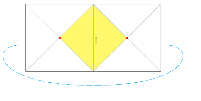
Figure 2: Conformal diagram for 2-D de Sitter space and the static patch defined by a past and future pair of asymptotic points. The static patch (yellow) is the intersection of the causal future of the past point and the causal past of the future point. The intersection of the two light cones shown as red dots defines the bifurcate horizon. The dashed blue curve indicates identification of the left and right edges.

A static patch is defined by picking a pair of points, one on the asymptotic past and one on the asymptotic future. The static patch is the intersection of the causal future of the past point and the causal past of the future point. The geodesic connecting the asymptotic points will be referred to as the world-line of the “pode.”

Observers who spend their entire existence in the static patch will see their world bounded by the horizon although the full geometry has no boundary. Our central hypothesis is that everything that goes on in the static patch can be described by a unitary holographic system with the degrees of freedom located at the stretched horizon (see section 2.2). The holographic quantum mechanics, which includes a Hilbert space and a Hermitian Hamiltonian, allows us to define certain thermal properties of the static patch including a density matrix, a temperature $T=1/\beta$, and an entropy $S_{0}$.

$$\rho = \frac{e^{-\beta H}}{Z}$$ (2.4)

$$\beta = \frac{1}{T}=2\pi R$$ (2.6)

$$S_{0} = \rm Tr\it\ \rho\log{\rho}=\frac{\pi R^{2}}{G}$$ (2.8)

In addition to the quantum mechanics of a single static patch, we also require transformation laws between static patches. For example in fig 3 we see two static patches of $dS_{2}$.

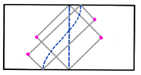
Figure 3: Two static patches in the same dS.

A theory of de Sitter space  should have transformation rules relating conditions in different static patches. In classical GR these transformations are symmetries that express the identical nature of the patches. These symmetries relating static patches, and the possibility of representing them in a holographic theory are the main subject of this paper.

The Penrose diagram for general dimensional de Sitter space is shown in the top panel of fig 4.

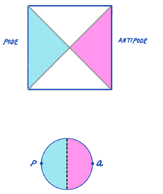
Figure 4: Upper panel: Penrose diagram for higher dimensional de Sitter space. Static patches come in pairs and the center of these patches are referred to as the pode and the antipode. Lower panel: the geometry of the $t=0$ slice of de Sitter space  is a sphere with the pode at one pole and the antipode at the other. The dashed surface midway between the pode and antipode is the bifurcate horizon.

The diagram shows that static patches come in matched pairs—blue and pink in the diagram. We will refer to the points at the centers of these static patches as the pode and the antipode.

2.2 Where is the Hologram?

The penrose diagram of fig 4 looks a lot like the diagram for the two-sided AdS eternal black hole [10]. From all that we know about such black holes this suggests (and we will assume) that the podal and antipodal degrees of freedom  are uncoupled, but entangled in a thermofield-double state. However the geometries of the two-sided black hole and de Sitter space are very different. In the lower panel of fig 4 we see a time-symmetric slice through the de Sitter space  geometry at $t=0.$ The geometry of the slice is a sphere. By contrast the corresponding slice through the eternal black hole would be a wormhole connecting two infinite asymptotic boundaries. The spatial slice of de Sitter space  has no boundary, the pode and antipode being points at which the geometry is smooth.

Instead of being located at the boundary as in AdS the holographic degrees of freedom  of the static patch are located at the (stretched) horizon. To see this, consider Bousso’s generalization [11] of the Penrose diagrams for the AdS eternal black hole, and for de Sitter space These are shown in fig 5.

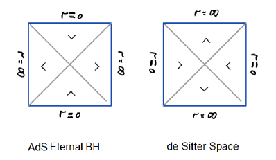
Figure 5: Penrose diagrams supplemented with Bousso wedges for the AdS eternal black hole and for de Sitter space  .

The question is: Where should we locate the holographic screens (tips of the wedges) so that the maximum entropy of the spatial region described by the hologram is sufficient to encode everything in the geometry? In fig 6 the diagrams are shown for AdS in which we place the screens near the horizon in the first case and near the boundary in the second case.

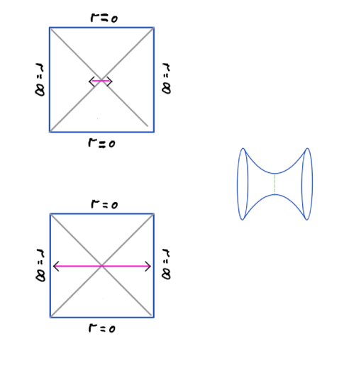
Figure 6: The AdS eternal black hole case: the upper panel introduces screens close to the horizon. According to the light-sheet entropy bound the number of degrees of freedom   on the screens is sufficient to represent the states of the black hole, but not sufficient to represent degrees of freedom  in the space far from the horizons. In the lower panel the screens are placed out near the AdS boundaries. In this case the degrees of freedom  on screens is sufficient to encode the entire space.

From the light-sheet entropy bounds of [12][11] one sees that in the first case the maximum entropy on the pink spatial region is just a tiny bit larger than the black hole entropy. Placing holographic degrees of freedom at these locations would allow enough degrees of freedom to describe the black hole, but not enough to describe phenomena in the bulk far from the horizon.

In the second case, where the wedges are near the boundary, the maximum entropy grows as the screens are moved outward. This is the well-known reason that the holographic degrees of freedom of AdS are located at the boundary.

Next consider de Sitter space. In figure 7 two choices for the locations of holographic screens are shown. In the upper panel the screen is shown near the pode.

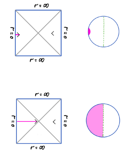
Figure 7: Penrose-Bousso diagrams for de Sitter space  . In the upper panel the screen is near the pode and the screen has almost no degrees of freedom . In the lower panel the screen is near the horizon and the number of degrees of freedom  is sufficient to encode the entire static patch.

The maximum entropy is very small when the screen is near the pode. By contrast, in the lower panel the screen is shown close to the horizon.The maximum entropy on the pink slice in this case is large enough to describe the entire static patch.That’s the argument for locating the holographic degrees of freedom  at the horizon.

The Penrose diagram suggests that there are two sets of degrees of freedom—one for the pode and one for the antipode—located on the stretched horizons of each side, and entangled in a thermofield-double state (see fig 8).

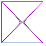
Figure 8: The stretched horizons of the pode and antipode patches.

2.3 Symmetry of De Sitter Space

Let’s suppose that an oracle handed us what he claimed is a holographic dual of de Sitter space. How would we know if it really describes de Sitter space  or something else—perhaps a black hole? The answer is symmetry. There are many static patches in de Sitter space  and the symmetry of the space transforms one to another. The most conclusive test would be to show that the model satisfies the de Sitter space  symmetry. In figure 3 we see that one static patch can probe the region behind the horizon of another. Since the original pode-patch is described by unitary evolution, establishing that the symmetry is satisfied would tell us that all static patches are described by unitary evolution. To put it another way, testing the de Sitter symmetry is also testing for the existence of space-time behind the horizon. Without testing the symmetry there is no compelling reason to think that a given quantum system represents dS.

The symmetry of clasical $d$-dimensional de Sitter space is $O(d,1),$ a non-compact version of the orthogonal group $O(d+1).$ $O(d,1)$ has

$$\frac{d(d+1)}{2}$$

generators. Of these

$$\frac{(d-2)(d-1)}{2}+1$$

generate transformations that keep the pode, antipode, and the horizon fixed. I’ll refer to these as the “easy” generators. They include rotations $R$ about the pode-antipode axis and the boost-Hamiltonian $H.$

In addition there are $(d-1)$ rotations ${\cal{J}}$, which rotate the positions of the pode and antipode, and another $(d-1)$ boost operators ${\cal{K}}$, that also move the pode, antipode, and horizon. I’ll call these the “hard” generators.

As an illustration here is the complete algebra for $d=3$,

$$[R,H] = 0$$ (2.9)

$$[R,{\cal{J}}] = i\epsilon_{ij}{\cal{J}}_{j}$$ (2.11)

$$[R,{\cal{K}},] = i\epsilon_{ij}{\cal{K}}_{j}$$ (2.13)

$$[{\cal{J}}_{i},{\cal{J}}_{j}] = i\epsilon_{ij}R$$ (2.15)

$$[{\cal{K}}_{i},{\cal{K}}_{j}] = -i\epsilon_{ij}R$$ (2.17)

$$[{\cal{J}}_{i},{\cal{K}}_{j}] = i\epsilon_{ij}H$$ (2.19)

$$[H,{\cal{K}}_{i}] = -i\epsilon_{ij}{\cal{J}}_{j}$$ (2.21)

$$[H,{\cal{J}}_{i}] = i\epsilon_{ij}{\cal{K}}_{j}$$ (2.23)

2.4 Four Step Protocol

What follows is a schematic protocol to test the oracle’s claim. If it succeeds then the oracle’s purported dual is legitimate. If it fails then we know he is a phony.

Actually there is a middle ground. Suppose the protocol succeeds to some very high level of accuracy, but beyond that it fails. Then the right thing to do is to see if the small violations have a plausible gravitational explanation. As we will see this is not just an academic possibility.

The protocol is probably consistent at the semiclassical level—in other words to all orders in perturbation theory. Beyond that, at the level of exponentially small non-perturbative effects, the protocol must fail, but there is a plausible gravitational explanation for the failure involving higher genus saddle points in the gravitational path integral.

To formulate the protocol we first break the de Sitter symmetry by choosing a pair of static patches, the pode and the antipode. This is not a real symmetry breaking; in the semiclassical theory it is gauge fixing. If the theory is gauge invariant then the results of any physical calculation should not depend on the gauge, which in this case means the particular pair of asymptotic points used to define the static patch.

1. Step one begins with a candidate for the dual of the static patch. It consists of a conventional quantum system: a Hilbert space ${\cal{H}}_{{\bf{p}}}$ of states; a Hamiltonian $H_{{\bf{p}}}$; and a set of Hermitian observables including the easy generators of the subgroup that hold fixed the pode. These generators include the Hamiltonian $H_{{\bf{p}}}$ and the rotation generators $R_{\bf{p}}$ that rotate the static patch around the pode. The easy generators are collectively denoted $G_{\bf{p}}.$

   The system is assumed to be in thermal equilibrium at some definite temperature $T$ and entropy $S.$

2. Step two introduces another copy of the system labeled ${\bf{a}}$ (for antipode). The doubled system has Hilbert space

   $${\cal{H}}={\cal{H}}_{{\bf{p}}}\otimes{\cal{H}}_{{\bf{a}}}.$$ (2.24)

   The total Hamiltonian is,

   $$H=H_{{\bf{p}}}-H_{{\bf{a}}}.$$ (2.25)

   The Hamiltonian $H_{{\bf{a}}}$ is identical to $H_{\bf{b}}$. The full Hamiltonian generates a boost that translates one side of the Penrose diagram (the pode side) upward, and the other side downward.

   The full rotation generators acting on ${\cal{H}}$ are

   $$R=R_{{\bf{a}}}+R_{\bf{b}}.$$ (2.26)

   More generally,

   $$G=G_{{\bf{a}}}\pm G_{\bf{b}},$$ (2.27)

   the minus sign being chosen for the Hamiltonian.

   Because de Sitter space  is spatially closed without a boundary we must impose gauge constraints,

   $$G|\Psi\rangle=0$$ (2.28)

   on the physical states.

   So far none of this is unusual and can easily be satisfied in many ways. That’s why I call $G$ the “easy” generators. Another way to characterize them is that they are the generators that commute with the Hamiltonian. And finally the easy generators do not couple the pode and antipode degrees of freedom.

3. The third step involves the construction of the remaining “hard” generators of $O(d,1)$, those that displace the pode and antipode. Let us call them ${\cal{G}}.$ They consist of the remaining rotation generators ${\cal{J}}$ and an equal number of boosts ${\cal{K}}$. The hard generators couple the pode and antipode degrees of freedom non-trivially. The easy and hard generators together form the $O(d,1)$ algebra.

   This third step may not be possible. There may be no choice of ${\cal{G}}$ that satisfies the commutation relations 3.45. This in itself may not be fatal if the algebra can be realized to a sufficiently high degree of accuracy. For example the violations may be exponentially small $\sim\exp{(-S_{0})}$. The symmetry may be satisfied to leading order in an expansion in $e^{-S_{0}}$, with the violations occurring only in higher orders. We will see in section 5.1 that this is exactly what the GKS anomaly tells us must happen. But for now let us assume the ${\cal{G}}$ can be constructed.

4. The final step, assuming the others have been successful, is to impose the hard gauge constraints,

   $${\cal{G}}|\Psi\rangle=0.$$ (2.29)

   Note that the hard gauge constraints 2.29 automatically imply the easy gauge constraints 2.28 but not the other way. As in step 3, if the entropy is finite this may only be possible to exponential precision.

If there are no states satisfying the gauge constraints,

$$G|\Psi\rangle = 0$$ (2.30)

$${\cal{G}}|\Psi\rangle = 0,$$ (2.32)

then we stop, go back, and choose another candidate until we find one that has at least one gauge-invariant state.

The gauge invariant state that is crucial is the de Sitter vacuum which looks thermal to observers in the pode and antipode patches. This state is the thermofield-double,

$$|TFD\rangle=\sum_{i}e^{-\frac{\beta E_{i}}{2}}|E_{i}\rangle_{{\bf{a}}}|{\bar{E}}_{i}\rangle_{\bf{b}}.$$ (2.33)

which must satisfy the gauge constraints, at least to leading order in $\exp{(-S_{0})}$. I don’t see any reason why there should be other gauge invariant states but this seems to be controversial. In any case the entire discussion in this paper is about the state in 2.33.

We will return to these symmetry issues but first I want to digress and describe a toy model which can provide a source of intuition about de Sitter static patches.

3 Toy Model

The motivation for the toy model is the observation that the pode is a point of unstable equilibrium. Imagine a light test-particle located exactly at the pode. Consider a second test-particle a tiny distance from the pode. Assume the second particle is initially at rest relative to the pode and subsequently follows a geodesic. Geodesic deviation will cause that particle to fall away from the pode with the separation growing exponentially. This is illustrated in fig 9.

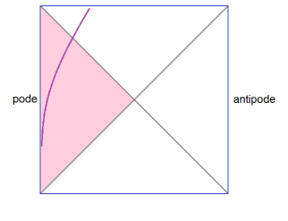
Figure 9: The pode is a point of instability. A particle arbitrarily close to the pode will depart (exponentially) from the pode and eventually it will fall through the horizon. Classically it will take a logarithmically infinite coordinate time to reach the horizon.

To model this behavior we can consider a non-relativistic particle in an inverted three-dimensional harmonic oscillator potential,

$$H=\sum_{i}\frac{p_{i}^{2}-x_{i}^{2}}{2}\ \ \ \ \ \ \ \ \ (i=1,2,3)$$ (3.34)

The unstable equilibrium point $x_{i}=0$ corresponds to the pode. The spectrum of $H$ is continuous and runs over all real numbers. The energy eigenfunctions at large $x$ have the form,

$$\psi\to e^{\pm ix^{2}/2}.$$ (3.35)

Classically, if the particle starts near the top of the potential the subsequent motion satisfies,

$$r \equiv \sqrt{|x|^{2}}\to e^{t}$$ (3.36)

$$|p| \to e^{t},$$ (3.38)

where $p$ is the momentum of the particle. This matches the behavior of a particle in dS.

The time that it takes for the particle to get to distance $R$ from the pode is,

$$t_{*}\approx\log R.$$ (3.39)

I’ve intentionally used the notation $t_{*}$ which is the conventional notation for the scrambling time. The reason will become clear shortly.

The inverted oscillator is characterized by an operator algebra including the Hamiltonian, and for each direction a generator $L_{\pm}$ defined by,

$$L_{\pm}=\frac{x\pm p}{\sqrt{2}}.$$ (3.40)

The algebra, which I will call the symmetry of the model is,

$$[H,L_{-}] = iL_{-}$$ (3.41)

$$[H,L_{+}] = -iL_{+}$$ (3.43)

$$[L_{-},L_{+}] = i.$$ (3.45)

From the first two of these relations it follows that,

$$L_{-}(t) = L_{-}e^{-t}$$ (3.46)

$$L_{+}(t) = L_{+}e^{t}$$ (3.48)

The algebra is satisfied by a generalization to a system of many non-interacting particles as well as particles coupled by translationally invariant forces.

The toy model as defined up to this point is the semiclassical limit of a more complete model which has a stretched horizon, a finite entropy, and nonperturbative effects.

3.1 Toy Model with Stretched Horizon

So far, in the toy model the particle falls in the potential for an infinite amount of time before reaching $r=\infty$. This parallels the fact that classically, a particle takes infinite time to reach the de Sitter horizon.

To make a more interesting model the radial direction can be cut off by turning the potential sharply upward at a distance $R$ from the pode. Instead of a single particle we can introduce $N$ particles which are allowed to interact, but only when they are very near the bottom of the potential. The details of the interaction are not important other than they lead to chaotic behavior and thermalization.

Figure 10 illustrates the setup. The first panel shows the potential, along with $N$ particles in thermal equilibrium at the bottom. The second panel is the view-from-above in which we see the particles occupying a two-dimensional shell at distance $R$ from the pode. This shell is the toy model version of the stretched horizon.

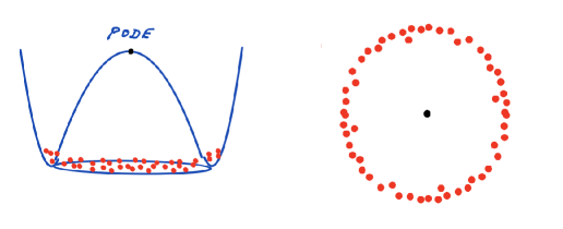
Figure 10: Toy model with stretched horizon. The right panel shows the view from above.

The number of particles can be chosen so that the area-density at the stretched horizon is of order $1/G.$ The entropy of the thermal gas is proportional to the number of particles and and by an appropriate choice of temperature and other numerical constants,

$$S_{0} = \frac{\rm Area}{4G}$$ (3.49)

$$= \frac{\pi R^{2}}{G}$$ (3.51)

Note that the time that it takes for a particle to fall from the pode to the stretched horizon is the scrambling time.

The semiclassical limit is identified with the limit $R\to\infty.$ In that limit the entropy becomes infinite and the thermal state is very boring to an observer at the pode. Thermal fluctuations do occur, but the potential well is so deep that the probability for a particle in the equilibrium “soup” to reach the pode is zero.

3.2 Fluctuations

If $R$ (and therefore the entropy) is kept finite, there is a non-zero probability to find one or more particles at the pode. The particles could form interesting objects such as black holes, galaxies, or brains. These nonperturbative Boltzmann fluctuations are extremely rare, but they are the only things that happen in thermal equilibrium [8].

Consider the probability of a Boltzmann fluctuation in which an object ${\cal{O}}$ materializes at the pode. To represent this situation mathematically we introduce a projection operator $\Pi_{{\cal{O}}}$ that projects onto states in which the object ${\cal{O}}$ is present at the pode. The probability in question is given by,

$$P_{{\cal{O}}}=Tr\ \rho\Pi_{{\cal{O}}}$$ (3.52)

where $\rho$ is the thermal density matrix.

Non-equilibrium dynamics is encoded in the thermal state. For example, suppose we want to know the probability that if the object ${\cal{O}}$ is present at $t=0,$ then at a later time $t$ it will have made a transition to ${\cal{O}}^{\prime}.$ This is encoded in the correlation function,

$$Tr\rho\ \Pi_{{\cal{O}}}\ e^{-iHt}\ \Pi_{{\cal{O}}^{\prime}}\ e^{iHt}=Tr\rho\ \Pi_{{\cal{O}}}(0)\ \Pi_{{\cal{O}}^{\prime}}(t)$$ (3.53)

This type of formula, and generalizations of it, show that the theory of fluctuations in thermal equilibrium encodes a very rich spectrum of dynamical phenomena.

The probability $P_{{\cal{O}}}$ is given by a standard expression,

$$P_{{\cal{O}}}=e^{-\Delta S}$$ (3.54)

where the “entropy-deficit”  $\Delta S$ is defined by,

$$\Delta S=S_{0}-S_{{\cal{O}}}.$$ (3.55)

This formula requires some explanation. The symbol $S_{0}$ stands for the de Sitter entropy $\pi R^{2}/G.$ $S_{{\cal{O}}}$ however, does not stand for the entropy of the object ${\cal{O}}.$ It is the conditional entropy of the whole system, given that the object ${\cal{O}}$ is present at the pode. A simple way to think about $S_{{\cal{O}}}$ is that it represents the entropy of the remaining horizon degrees of freedom, given that ${\cal{O}}$ is present, plus the entropy of ${\cal{O}}.$ We will return to this in section 5.2.

3.3 The GKS Anomaly

Can the algebra 3.45 be satisfied in the cutoff model? With the identification 3.40 and the modification of the Hamiltonian required to construct the cutoff model, the algebra will not hold, but one may ask if there can be new operators $L_{\pm}$, which along with the new Hamiltonian, satisfy it? The answer is no [1]. To prove it we consider the first of equations 3.48 (a consequence of the algebra) and take its matrix element between normalizable states,

$$\langle\psi|L_{-}(t)|\psi\rangle\to e^{-t}\to 0.$$ (3.56)

The argument for the GKS anomaly contains two parts:

1. Finiteness of entropy implies that the energy spectrum is discrete. More exactly it says that the number of states below any given energy is finite. This is much weaker than saying the Hilbert space is finite dimensional, which we do not assume.

2. Functions defined as sums of the form,

   $$F(t)=\sum_{i}a_{i}e^{iE_{i}t}$$ (3.57)

   cannot go to zero as $t\to\infty.$ They will have fluctuations and even recurrences on very long time scales. One can easily prove that the late-time variance of $F(t)$ satisfies,

   $$\lim_{T\to\infty}\frac{1}{T}\int_{0}^{T}|F^{2}|dt=\sum_{i}|a_{i}|^{2}>0$$ (3.58)

   In other words, over long periods of time $F$ will fluctuate with a variance equal to $\sum_{i}|a_{i}|^{2}.$

It follows [1] that 3.56 (and the algebra 3.45 which led to it) cannot be satisfied if the entropy is finite. There is a deep relationship between fluctuations and the non-perturbative breaking of semiclassical symmetries.

We can be more quantitative. In the semiclassical limit the energy spectrum is continuous and 3.57 is replaced by,

$$F(t)=\int A(E)e^{iEt}.$$ (3.59)

If $A(E)$ is square integrable then $F(t)\to 0$ as $t\to\infty.$ In approximating the sum by an integral we make the following correspondence:

$$a_{i}=A(E)\delta E$$ (3.60)

where $\delta E$ is the spacing between neighboring energy levels. Now consider the sum in 3.58 and rewrite it in terms of $A$.

$$\sum|a_{i}|^{2} = \sum|A(E)|^{2}(\delta E)^{2}$$ (3.61)

$$\to \int|A(E)|^{2}\delta EdE$$ (3.63)

The energy level spacings $\delta E$ are of order $e^{-S_{0}}.$ Thus it follows that $|\sum a_{i}|^{2}\sim\delta E\sim e^{-S_{0}},$ and from 3.58,

$$\rm Var\it(L_{-})\sim e^{-S_{0}}.$$ (3.64)

Given that the symmetry algebra requires the asymptotic variance in $L_{-}$ to be zero, the actual variance in 3.64 is a measure of how badly the symmetry is broken by the anomaly.

More generally it seems reasonable to suppose that the discreteness of the energy spectrum produces effects that scale like a power of $e^{-S_{0}}.$

The bottom line is that fluctuations of order $e^{-S_{0}}$ create an obstruction to realizing the symmetry algebra 3.45 as long as the entropy is finite.

3.4 Caveats

The toy model has elements in common with de Sitter space, but like all analogies it has limitations. Two come to mind: First, because it is based on non-relativistic particles it cannot capture the physics of massless photons in de Sitter space. For example the probability to find a single thermal photon of wavelength $\sim R/2$ within a distance $\sim R/2$ of the pode is order $1.$ This is a perturbative phenomenon which would requires massless relativistic degrees of freedom instead of massive non-relativistic particles.

Another unphysical feature of the toy model is that the size of the horizon is fixed, while the size of the de Sitter horizon is dynamical and adjusts to the amount of entropy that it contains (see section 5.2).

4 The GKS Anomaly in JT/SYK

A similar anomaly to that seen in section 3.3 also affects two-dimensional models such as JT gravity and its quantum SYK completion. Figure 12 shows the $AdS(2)$ solution of JT gravity with its Rindler-like horizons.

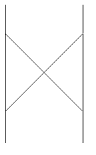
Figure 11: $AdS(2)$ with horizons.

The classical theory has an exact $SL(2R)$ symmetry which persists to all orders in perturbation theory; in other words it is a feature of the semiclassical theory. However the symmetry is broken by non-perturbative quantum effects [13]. The $SL(2R)$ group has three generators, ${\cal{T}},H$ and ${\cal{P}},$ whose action is illustrated diagramatically [14] in the three panels of fig 12.

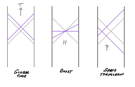
Figure 12: The three generators of $SL(2R)$: ${\cal{T}}$ generates global time translations and shifts the horizon vertically; $H$ is the boost Hamiltonian that generates Rindler-like boosts; and ${\cal{P}}$ generates space-like shifts of the horizon. Only $H$ does not move the horizon.

The generator ${\cal{T}}$ generates global time shifts and moves the horizons vertically from their original location (grey lines) to a new location (purple lines.) The generator $H$ is the boost Hamiltonian that holds the horizons fixed but acts on equal-time-slices to boost them. Finally ${\cal{P}}$ generates a spacelike displacement of the horizon as shown. ${\cal{T}}$ and ${\cal{P}}$ are analogous to the hard generators of $O(d,1)$ and $H$ is easy.

These generators satisfy the $SL(2R)$ algebra,

$$[H,{\cal{T}}] = i{\cal{P}}$$ (4.65)

$$[H,{\cal{P}}] = i{\cal{T}}$$ (4.67)

$$[{\cal{T}},{\cal{P}}] = iH$$ (4.69)

which as I said is exact semiclassically, but cannot hold non-perturbatively. To see this we define the light-like generators,

$$L_{-} = \frac{{\cal{P}}-{\cal{T}}}{\sqrt{2}}$$ (4.70)

$$L_{+} = \frac{{\cal{P}}+{\cal{T}}}{\sqrt{2}}.$$ (4.72)

From 4.69,

$$i[H,L_{\pm}]=\pm L_{\pm}$$ (4.73)

implying,

$$L_{\pm}(t)=L_{\pm}e^{\pm t}.$$ (4.74)

In the classical JT system the entropy is infinite and equation 4.74 presents no problem, but in a quantum completion such as SYK the entropy is finite, of order the number of fermion species $N.$ The rest of the argument is identical to the one in section 3.3 and implies that the $SL(2R)$ symmetry cannot be exact, except in the limit $N\to\infty.$

All of this is well known from other points of view [13] [14], and it is believed that the breaking of the symmetry can be understood in terms of higher genus corrections to the JT path integral.

5 de Sitter

Return now to de Sitter space and static patch holography. In so far as the static patch is in thermal equilibrium with finite entropy it will undergo Boltzmann fluctuations. As we saw in section 3.3 these fluctuations are the source the symmetry breaking in the toy model. In this section I’ll do two things: first I’ll discuss the anomaly in the $O(d,1)$ de Sitter symmetry; and then I’ll explain how general relativity can be used to give a quantitative account of Boltzmann fluctuations

5.1 The O(d,1) Anomaly

Now let’s return to the symmetry algebra of de Sitter space. From the last two of equations 2.23 we may construct light-like generators,

$$L_{\pm}=\frac{{\cal{J}}_{2}\pm{\cal{K}}_{1}}{\sqrt{2}}$$ (5.75)

satisfying,

$$i[H,L_{\pm}]=\pm L_{\pm}.$$ (5.76)

Note that these equations are identical to the first two equations in 3.45 and that they again imply,

$$L_{-}(t)=L_{-}(0)e^{-t}.$$ (5.77)

Following the same logic as in section 3.3 we may evaluate this equation between normalizable states to find,

$$\langle\psi|L_{-}(t)|\psi\rangle\to 0.$$ (5.78)

For the same reasons as in 3.3 and in [1] (having to do with persistent fluctuations) there is a GKS anomaly making it impossible to satisfy 5.78, and therefore the algebra. The arguments of section 3.3 concerning fluctuations give the same estimate for the magnitude of the effects of the anomaly,

$$\rm Var\it(L_{-})\sim e^{-S_{0}}.$$ (5.79)

5.2 Using GR to Calculate Fluctuation Probabilities

In theories with a gravitational dual, general relativity provides a precise way of calculating the probability for certain fluctuations. Consider the rate for fluctuations which nucleate massive objects such as black holes near the pode. We may make use of 3.54 and 3.55 to compute the rate. To calculate $S_{0}$ we can use the metric 2.3 to get the radius of the horizon (we get $r_{H}=R$), then calculate the area of the horizon, and finally the entropy. The result is,

$$S_{0}=\frac{\pi R^{2}}{G}.$$ (5.80)

Next consider the metric of de Sitter space with an object ${\cal{O}}$ of mass $M$ at the pode. The effect of the mass is to pull in the cosmic horizon, shrinking its area and therefore its entropy [15][16][17]. Out beyond the radius of the object the metric takes the form 2.3 except that the emblackening factor $f(r)$ is replaced by

$$f_{M}(r)=\left(1-\frac{r^{2}}{R^{2}}-\frac{2MG}{r}\right).$$ (5.81)

The horizon location is defined by $f_{M}(r)=0.$ Multiplying by $r$ this becomes,

$$r-\frac{r^{3}}{R^{2}}-2MG=0$$ (5.82)

Equation 5.82 has three solutions, two with positive $r$ and one with negative $r.$ The negative solution is unphysical. The larger of the two positive solutions determines the location of the cosmic horizon and the smaller determines the horizon of a black hole of mass $M$. To lowest order in $M$ the cosmic horizon is shifted to a new value of $r$ given by,

$$r=R-MG$$ (5.83)

The entropy is given by,

$$S_{{\cal{O}}}=\frac{\pi(R-MG)^{2}}{G}$$ (5.84)

and (to leading order in $M$) the entropy-deficit by [15],

$$\Delta S=2\pi MR.$$ (5.85)

Now recall that the inverse temperature of de Sitter space  is $\beta=2\pi R.$ Using 3.54 we find,

$$P_{{\cal{O}}}=e^{-\beta M}.$$ (5.86)

Equation 5.86 is the Boltzman weight of the for a configuration of energy $M.$ The answer itself is not surprising but what is interesting is that the connection between entropy and area has been used in a new way—not for equilibrium probabilities but for fluctuations away from average behavior.

More generally we can go past linear order in $M$. Let us denote the two solutions of 5.82 by $r_{-}$ and $r_{+}$ and define the independent parameter,

$$x=(r_{+}-r_{-}).$$ (5.87)

One can express $x$ in terms of the mass of the black hole by eliminating $r_{+}$ and $r_{-}$ from the equations,

$$R^{2} = r_{+}^{2}+r_{-}^{2}+r_{+}r_{-}$$ (5.88)

$$2MGR^{2} = r_{+}r_{-}(r_{+}+r_{-})$$ (5.89)

$$x = r_{+}-r_{-}$$ (5.90)

The value of $x$ runs from $(x=-R)$ to $(x=+R).$ Changing the sign of $x$ interchanges the cosmic and black hole horizons. It is convenient to think of positive and negative values of $x$ as different configurations; for example at both $x=-R$ and $x=+R$ there is a vanishingly small horizon and a maximally large horizon, but we regard the two states as different.

The entropy and entropy-deficit are given by

$$S_{\cal{O}} = \frac{\pi}{G}\left(r_{+}^{2}+r_{-}^{2}\right)$$ (5.91)

$$\Delta S = \frac{\pi}{G}\left(R^{2}-r_{+}^{2}-r_{-}^{2}\right)$$ (5.93)

Let us consider the “Nariai point” $(x=0)$ at which $(r_{+}=r_{-}).$ One easily finds that at the Nariai point,

$$r+^{2} = r_{-}^{2}$$ (5.94)

$$\equiv r_{N}^{2}$$ (5.96)

$$= \frac{R^{2}}{3}$$ (5.98)

From 5.93 and 5.98 we find,

$$S_{N} = \frac{2S_{0}}{3}$$ (5.99)

$$\Delta S_{N} = \frac{S_{0}}{3}$$ (5.101)

It is not obvious that $\Delta S$ is smooth at $x=0$. One might expect that $\Delta S(x)$ has a cusp as in the top panel of fig 13. However explicit calculation shows that the dependence is completely smooth and surprisingly simple,

$$\Delta S=\frac{S_{0}}{3}\left(1-\frac{x^{2}}{R^{2}}\right).$$ (5.102)

This is illustrated in the bottom panel of fig 13.

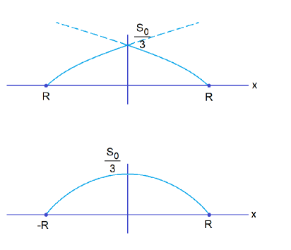
Figure 13: Entropy deficit and a function of $x$. The upper panel incorrectly shows a cusp at the Nariai point. The lower panel shows the correct smooth behavior 5.102.

The total probability for a black hole fluctuation is given by an integral over $x$,

$$\rm Prob\it = \frac{1}{R^{4}}\int_{0}^{R}e^{-\Delta S}x^{3}dx$$ (5.103)

$$= e^{\frac{-S_{0}}{3}}\frac{1}{R^{4}}\int_{0}^{R}e^{\frac{S_{0}x^{2}}{3R^{2}}}x^{3}dx.$$ (5.105)

One finds,

$$\rm Prob\it\sim\frac{3G}{\pi R^{2}}\left(1+\frac{3}{S_{0}}e^{-S_{0}/3}\right)$$ (5.106)

The first term in 5.106 comes from the endpoint of the integration at $x^{2}=R^{2}$ and is perturbative in $G.$ It is associated with the lightest black holes and numerically dominates the integral. The second term comes from the saddle point at $x=0.$ It can be re-written as

$$e^{-\frac{\pi R^{2}}{3}\frac{1}{G}}.$$

It is obviously non-perturbative in $G.$ We will discuss its meaning in the next section.

6 The Nariai Geometry

Quantum mechanically the non-perturbative fluctuations we are discussing originate from the discreteness of the energy spectrum. On the gravitational side those same effects are encoded in higher genus contributions to the gravitational (Euclidean) path integral [18][19][20][21][22]. In the case of anti de Sitter space the geometries that contribute are constrained to have asymptotic AdS-like boundary conditions, but subject to that constraint they can have any topology. In the case of Euclidean de Sitter space there are no boundaries; the path integral therefore includes all closed topologies. Among these are the Nariai geometries.

To illustrate the connection between fluctuations and higher-genus contributions consider the fluctuations discussed in section 5.2 in which a black hole is spontaneously created near the pode. The first panel of figure 14 shows the Penrose diagram for a Schwarzschild- de Sitter black hole. A slice through the time-symmetric space-like $t=0$ surface is depicted in green. In the lower panel the geometry of such a slice is shown for two different masses of the black hole. The figure on the right depicts a relatively larger mass than on the left.

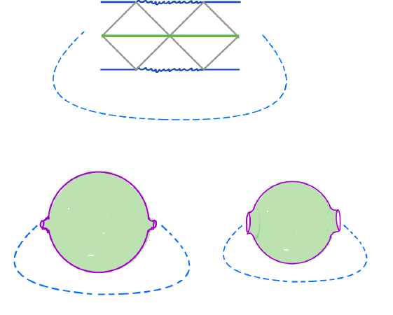
Figure 14: de Sitter-Schwarzschild black hole. The upper panel shows the Penrose diagram and the two lower panels show the spatial geometry of time-symmetric slices. In each case the dashed blue curves indicate geometric identifications.

One may continue the $t=0$ geometry in either Minkowski or Euclidean signature. The Minkowski continuation just gives back the geometry in the top panel of figure 14. The Euclidean continuation gives a compact geometry with the topology $S_{2}\times S_{2}$ which I will call an S-geometry (Euclidean Schwarzschild de Sitter). There is a one parameter family of S-geometries parameterized by the mass $M$ of the black hole.

The metric of the S-geometry is,

$$ds^{2}=\left(1-\frac{r^{2}}{R^{2}}-\frac{2MG}{r}\right)d\tau^{2}+\left(1-\frac{r^{2}}{R^{2}}-\frac{2MG}{r}\right)^{-1}dr^{2}+r^{2}d\Omega^{2}$$ (6.107)

The one thing left to specify is the range of the periodic Euclidean time $\tau.$ Normally the periodic constraint requires $0<\tau\leq\beta$ where $\beta$ signifies inverse temperature. However in the present case there is no well defined temperature because the black hole and cosmic horizon have very different temperatures. For a small black hole $\beta$ is $4\pi MG$ while the de Sitter value of $\beta$ is $2\pi R.$ The black hole is far out of equilibrium with the de Sitter space.

What this means geometrically is that it is not possible to avoid a conical singularity at either the black hole or the cosmic horizon. For this reason the S spaces are not genuine saddle points of the Euclidean gravitational path integral—with one exception. The exception is the Nariai space, i.e., S-space at the symmetric point $x=0.$ The geometry of Nariai space is $S_{2}\times S_{2}$ and its Minkowski continuation is $S_{2}\times dS_{2},$ i.e., a spatial sphere times two-dimensional de Sitter space.

Nariai space is a genuine Euclidean saddle point whose Minkowski continuation is often called the Nariai black hole. To understand it better let’s go back to S-space with a small black hole. A static patch is also shown in the upper panel of fig 15. Because the black hole is at the center of the static patch we cannot think of the pode as a point. Instead I’ve indicated a shell by a dashed red line. The shell is a 2-sphere that surrounds the black hole between the black hole horizon (black dot) and the cosmic horizon (purple dot).

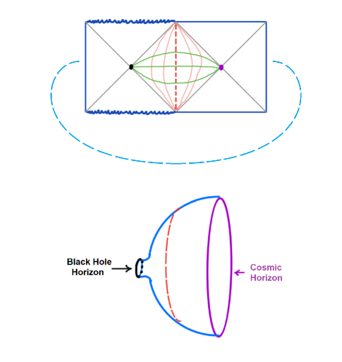
Figure 15: The top panel shows the penrose diagram for a Euclidean Schwarzschild black hole together with a static patch which encloses the black hole symmetrically. The black dot on the left is the black hole horizon. The purple dot on the right is the cosmic horizon. The lower panel shows a spatial slice of the region between the two horizons. The dashed red line indicates the static position of a $2$-sphere somewhere between the two horizons.

A spatial $t=0$ slice of the geometry between the two horizons is shown in the lower panel.

Now let us consider deforming the geometry by increasing the black hole mass and at the same time decreasing the cosmic horizon area (following the curve in the lower panel of fig 13) until we reach the Nariai point. At that point the geometry—not just the topology— is $S_{2}\times S_{2}$ but from the viewpoint of the static patch observer, it looks like a spatial interval times a $2$-sphere. The observer is sandwiched between two equal horizons.

Thought of as a real process, this history would violate the second law of thermodynamics, but as long as $S_{0}$ is finite, it can happen as a rare Boltzmann fluctuation. What it requires is for energy to be transferred from the cosmic horizon to the black hole—a kind of anti-evaporation. The most likely trajectory for the system to follow is the time reverse of the evaporation process in which one of the two Nariai horizons spontaneously emits a bit of radiation which is then absorbed by the other. When this happens the emitter loses energy and becomes hotter. The result is that it emits more energy until the smaller horizon becomes a small black hole (or even no black hole) and the larger horizon reaches entropy $S_{0}.$ The time reverse of this process is the Boltzmann fluctuation that leads to the Nariai state from the small black hole state.

Once the Nariai state is achieved it is unstable. One possibility is that the system can return to the original state with the original black hole shrinking and the original cosmic horizon returning to its full dS size. But the opposite can also happen: the system overshoots a bit and the original black hole keeps absorbing energy while the original cosmic horizon shrinks down to a small black hole. We can think of this as a transition from from $x=-R$ to $x=+R.$ An observer between the two horizons sees a surprising history in which the geometry of the static patch turns itself “inside-out”—the outer cosmic horizon and the inner black hole horizon exchanging roles. This remarkably strange event is illustrated in fig 16.

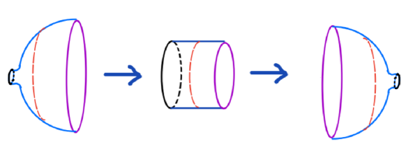
Figure 16: The “inside-out transition” in which a small black hole horizon and the cosmic horizon become interchanged by passing through the intermediate Nariai black hole.

6.1 Nariai and Hawking-Moss

One might be tempted to think of this inside-out transition as a quantum tunneling event, but unlike a typical quantum tunneling the process stretches out over a long time. The energy transfer is simply Hawking evaporation or its time-reverse, and takes a time of order the Page time. The transition is a thermal process mediated by a Hawking-Moss instanton[23], not a quantum tunneling event. It takes a very long time during which the system sits at or near the top of the potential, i.e, at $x=0$. The Hawking-Moss instanton calculates the probability that the system in question is at the top of a broad potential barrier [24].

In this case the Hawking-Moss instanton is the Nariai geometry, $S_{2}\times S_{2}$ and the probability to find the system in the Nariai state is

$$e^{-{\Delta I_{N}}}$$

where $I$ is the action-deficit of Euclidean Nariai space. Not surprisingly that action deficit is the same as the entropy-deficit of the Nariai black hole,

$$\Delta I_{N}=\frac{S_{0}}{3}.$$ (6.108)

Thus we see an example of the relation between fluctuations (The appearance of a Nariai black hole) and a higher genus wormhole geometry (the $S_{2}\times S_{2}$ Nariai geometry.)

6.2 Connection with Anomaly

What does all of this have to do with the $O(d,1)$ symmetry (or lack of it) of de Sitter space? I think the answer is fairly simple. In the Euclidean continuation the symmetry group is $O(5).$ There is a natural action of the $O(5)$ group on the semiclassical Euclidean dS geometry, namely $S_{4}$. But the full path integral receives contributions from other topologies, in particular the Nariai geometry $S_{2}\times S_{2}.$ Trying to define the action of $O(5)$ on $S_{2}\times S_{2}$ is like trying to define the action of $O(3)$ on a torus. It’s not that the torus breaks the symmetry like a egg would; the symmetry operations just don’t exist on the torus. Likewise the generators of $O(5)$ don’t exist on $S_{2}\times S_{2}.$

One might try to get around this by defining the action of the group to be trivial on all higher topologies; in other words define $S_{2}\times S_{2}$ to be invariant under $O(5).$ I think the reason that this doesn’t work is that in general, states of different topology are not orthogonal: the overlaps are order $\exp(-S)$ [21]. For this reason the action of the group on $S_{2}\times S_{2}$ cannot be arbitrarily chosen independently of the action on $S_{4}.$

Thus we are left with the conclusion that higher topologies not only break the symmetry of dS: they don’t even allow it to be defined. This is consistent with the GKS anomaly which also implies that the generators cannot consistently be constructed to order $\exp{(-S_{0})}$.

7 Implications of the Anomaly

The group $O(d,1)$ relates different static patches within a single de Sitter space. For example in fig 17 shows two static patches related by the action of a light-like generator $L.$

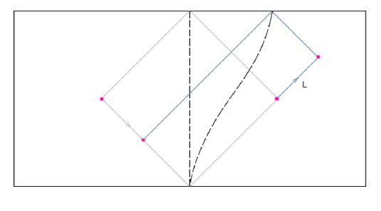
Figure 17: Two-dimensional de Sitter space  with two static patches related by a light-like generator $L.$

If the $O(d,1)$ symmetry were not broken by the GKS anomaly one would expect that the dynamics in the two patches would be identical. In particular the Hamiltonian in one patch would be related to that in the other patch by a unitary transformation and the two spectra would be identical. However our result suggests that this is not true; what is more likely is that the coarse-grained spectra of the two Hamiltonians are the same but at the discrete level of individual eigenvalues, the spectra do not match. The occurrence and timing of fluctuations in the two static patches (for example quantum recurrences) would be different. The Hamiltonians for different patches might be drawn from a single ensemble but would be different instances of that ensemble. In the absence of knowledge about which Hamiltonian governs an observer’s patch, averaging over the ensemble would make sense.

7.1 Gauge Symmetry?

It is usually assumed that the $O(d,1)$ relating different static patches is a gauge symmetry, or a redundancy of the description. But having a gauge symmetry requires that the gauge transformation can be consistently defined. This does not appear to be possible for the symmetries of de Sitter space except in the semiclassical limit. The GKS anomaly precludes the existence of the generators to higher order in $e^{-S_{0}}$ and indicate the different static patches are inequivalent when effects of order $e^{-S_{0}}$ are considered. Thus, the answer to the question is that $O(d,1)$ should be treated as a gauge symmetry in the semiclassical approximation, but not in the full non-perturbative theory. One could select a static patch not by gauge fixing, but by simply selecting the patch whose detailed energy levels have some specific pattern.

One possible conclusion is that eternal de Sitter space is not consistent—a view taken in [1]. In this paper I’ve advocated another viewpoint; namely that the de Sitter symmetries are approximate, valid in classical theory and in perturbation theory, but not beyond. In fact for other topologies the action of $O(d,1)$ may not even be defined. For example it is hard to imagine the action of $O(d,1)$ on the Nariai space $S(2)\times S(2).$

In some ways the situation seems similar to recent discussions of global symmetries and their breaking by higher topologies [27] where it was suggested that global symmetries (forbidden by gravity) may be restored in the ensemble average. In the context of de Sitter space  the average over all the static patches in de Sitter space  might have the symmetry that the individual instances don’t have.

8 Conclusion

Eternal de Sitter space is a spacetime without time-like boundaries, but a static patch is bounded by a horizon. On the basis of covariant entropy bounds I argued that the natural place to locate holographic degrees of freedom is on the stretched horizon. The only things that happen in eternal de Sitter space are fluctuations of these horizon degrees of freedom, which from the bulk point of view sporadically produce interesting objects deep in the interior of the static patch.

We’ve explored three non-perturbative de Sitter space phenomena, related to these fluctuations. The first: the violation of the de Sitter symmetry $O(4,1)$ due to the GKS anomaly. The variance $\rm Var\it(L_{-})$ in 5.79 is a measure of the magnitude of the violation.

The second: large scale Boltzmann fluctuations in which the holographic horizon degrees of freedom undergo freak rearrangements, leading to large black holes materializing in the interior of the static patch. The probability for this to happen is given by 5.106. The second term of this expression is non-perturbative and represents the creation of the largest black holes with entropy $\approx S_{0}/3.$

Finally wormholes and higher genus geometries: a saddle point due to the Nariai geometry $S_{2}\times S_{2}$ contributes non-perturbatively to the gravitational path integral and describe a massive fluctuation in which de Sitter space turns itself “inside out.”

These phenomena which all scale exponentially with $-S_{0}$ are closely connected. One might even say they express the same underlying fact; namely the discreteness of the energy spectrum, and finite level spacing $\delta E\sim e^{-S}.$ Moreover they are extensions of things that have been observed in other contexts such as SYK and JT gravity. The new thing here is that they appear in the holography of de Sitter space.

The violation of symmetry is especially interesting. It means that different static patches are inequivalent. They may have different Hamiltonians and different energy spectra although the coarse grained spectra must be the same to insure a universal semiclassical limit. Although it is an open question, it is an interesting conjecture that the symmetry-violation is washed out by some form of ensemble averaging, as is thought to be the case for JT gravity.

References

- [1] N. Goheer, M. Kleban and L. Susskind, “The Trouble with de Sitter space,” JHEP 07, 056 (2003) doi:10.1088/1126-6708/2003/07/056 [arXiv:hep-th/0212209 [hep-th]].
- [2] R. Bousso, B. Freivogel and I. S. Yang, “Eternal Inflation: The Inside Story,” Phys. Rev. D 74, 103516 (2006) doi:10.1103/PhysRevD.74.103516 [arXiv:hep-th/0606114 [hep-th]].
- [3] D. Harlow, S. H. Shenker, D. Stanford and L. Susskind, “Tree-like structure of eternal inflation: A solvable model,” Phys. Rev. D 85, 063516 (2012) doi:10.1103/PhysRevD.85.063516 [arXiv:1110.0496 [hep-th]].
- [4] L. Susskind, “Fractal-Flows and Time’s Arrow,” [arXiv:1203.6440 [hep-th]].
- [5] L. Susskind, “Was There a Beginning?,” [arXiv:1204.5385 [hep-th]].
- [6] L. Susskind, “Is Eternal Inflation Past-Eternal? And What if It Is?,” [arXiv:1205.0589 [hep-th]].
- [7] L. Dyson, J. Lindesay and L. Susskind, “Is there really a de Sitter/CFT duality?,” JHEP 08, 045 (2002) doi:10.1088/1126-6708/2002/08/045 [arXiv:hep-th/0202163 [hep-th]].
- [8] L. Dyson, M. Kleban and L. Susskind, “Disturbing implications of a cosmological constant,” JHEP 10, 011 (2002) doi:10.1088/1126-6708/2002/10/011 [arXiv:hep-th/0208013 [hep-th]].
- [9] L. Susskind and E. Witten, “The Holographic bound in anti-de Sitter space,” [arXiv:hep-th/9805114 [hep-th]].
- [10] J. M. Maldacena, “Eternal black holes in anti-de Sitter,” JHEP 04, 021 (2003) doi:10.1088/1126-6708/2003/04/021 [arXiv:hep-th/0106112 [hep-th]].
- [11] R. Bousso, “A Covariant entropy conjecture,” JHEP 07, 004 (1999) doi:10.1088/1126-6708/1999/07/004 [arXiv:hep-th/9905177 [hep-th]].
- [12] W. Fischler and L. Susskind, “Holography and cosmology,” [arXiv:hep-th/9806039 [hep-th]].
- [13] J. Maldacena, D. Stanford and Z. Yang, “Conformal symmetry and its breaking in two dimensional Nearly Anti-de-Sitter space,” PTEP 2016, no.12, 12C104 (2016) doi:10.1093/ptep/ptw124 [arXiv:1606.01857 [hep-th]].
- [14] H. W. Lin, J. Maldacena and Y. Zhao, “Symmetries Near the Horizon,” JHEP 08, 049 (2019) doi:10.1007/JHEP08(2019)049 [arXiv:1904.12820 [hep-th]].
- [15] T. Banks, B. Fiol and A. Morisse, “Towards a quantum theory of de Sitter space,” JHEP 12, 004 (2006) doi:10.1088/1126-6708/2006/12/004 [arXiv:hep-th/0609062 [hep-th]].
- [16] L. Susskind, “Addendum to Fast Scramblers,” [arXiv:1101.6048 [hep-th]].
- [17] T. Banks and W. Fischler, “Holographic Space-time, Newton’s Law and the Dynamics of Black Holes,” [arXiv:1606.01267 [hep-th]].
- [18] J. S. Cotler, G. Gur-Ari, M. Hanada, J. Polchinski, P. Saad, S. H. Shenker, D. Stanford, A. Streicher and M. Tezuka, “Black Holes and Random Matrices,” JHEP 05, 118 (2017) [erratum: JHEP 09, 002 (2018)] doi:10.1007/JHEP05(2017)118 [arXiv:1611.04650 [hep-th]].
- [19] P. Saad, S. H. Shenker and D. Stanford, “A semiclassical ramp in SYK and in gravity,” [arXiv:1806.06840 [hep-th]].
- [20] P. Saad, “Black holes, baby universes, and random matrices,”
- [21] D. Marolf and H. Maxfield, “Transcending the ensemble: baby universes, spacetime wormholes, and the order and disorder of black hole information,” JHEP 08, 044 (2020) doi:10.1007/JHEP08(2020)044 [arXiv:2002.08950 [hep-th]].
- [22] A. Almheiri, R. Mahajan, J. Maldacena and Y. Zhao, “The Page curve of Hawking radiation from semiclassical geometry,” JHEP 03, 149 (2020) doi:10.1007/JHEP03(2020)149 [arXiv:1908.10996 [hep-th]].
- [23] S. W. Hawking and I. G. Moss, “Supercooled Phase Transitions in the Very Early Universe,” Phys. Lett. B 110, 35-38 (1982) doi:10.1016/0370-2693(82)90946-7
- [24] E. J. Weinberg, “Hawking-Moss bounces and vacuum decay rates,” Phys. Rev. Lett. 98, 251303 (2007) doi:10.1103/PhysRevLett.98.251303 [arXiv:hep-th/0612146 [hep-th]].
- [25] T. Banks, W. Fischler and S. Paban, “Recurrent nightmares? Measurement theory in de Sitter space,” JHEP 12, 062 (2002) doi:10.1088/1126-6708/2002/12/062 [arXiv:hep-th/0210160 [hep-th]].
- [26] T. Banks, “Some thoughts on the quantum theory of de sitter space,” [arXiv:astro-ph/0305037 [astro-ph]].
- [27] Y. Chen and H. W. Lin, “Signatures of global symmetry violation in relative entropies and replica wormholes,” JHEP 03, 040 (2021) doi:10.1007/JHEP03(2021)040 [arXiv:2011.06005 [hep-th]].