Amortized Generation of Sequential
Algorithmic Recourses for Black-box Models

Abstract

Explainable machine learning (ML) has gained traction in recent years due to the increasing adoption of ML-based systems in many sectors. Algorithmic Recourses (ARs) provide “what if” feedback of the form “if an input datapoint were $x^{\prime}$ instead of $x$, then an ML-based system’s output would be $y^{\prime}$ instead of $y$.” ARs are attractive due to their actionable feedback, amenability to existing legal frameworks, and fidelity to the underlying ML model. Yet, current AR approaches are single shot—that is, they assume $x$ can change to $x^{\prime}$ in a single time period. We propose a novel stochastic-control-based approach that generates sequential ARs, that is, ARs that allow $x$ to move stochastically and sequentially across intermediate states to a final state $x^{\prime}$. Our approach is model agnostic and black box. Furthermore, the calculation of ARs is amortized such that once trained, it applies to multiple datapoints without the need for re-optimization. In addition to these primary characteristics, our approach admits optional desiderata such as adherence to the data manifold, respect for causal relations, and sparsity—identified by past research as desirable properties of ARs. We evaluate our approach using three real-world datasets and show successful generation of sequential ARs that respect other recourse desiderata.

1 Introduction

Machine learning (ML) models are increasingly used to make predictions in systems that directly or indirectly impact humans. This includes critical applications like healthcare (Faggella 2020), finance (Singla 2020), hiring (Sennaar 2019), and parole (Tashea 2017). To understand ML models better and to promote their equitable impact in society, it is necessary to assess stakeholders’—both expert (Holstein et al. 2019) and layperson (Saha et al. 2020)—comprehension of and needs for general observability into their systems (Poursabzi et al. 2021; Ehsan et al. 2021a). The nascent Fairness, Accountability, Transparency, and Ethics in machine learning (aka “FATE ML”) community conducts research to develop methods to detect (and counteract) bias in ML models, develop techniques that make complex models explainable, and propose policies to advise and adhere to the regulations of algorithmic decision-making (see Appendix A). Here, we focus on ML model explainability.

Research in explainable ML is bifurcated. One high-level approach aims to develop inherently interpretable models such as decision trees and linear models (Rudin 2019). Another high-level approach aims to utilize existing complex classification techniques (such as deep neural networks) but to bolster them with surrogate models that can render their predictions and/or internal processes understandable (Adadi and Berrada 2018). This is achieved through explaining models holistically (global explanation) or single predictions from the model (local explanation).

Algorithmic Recourses (ARs). ARs find the minimal change in a datapoint such that the ML model ends up classifying the new datapoint in the desired class. Such new datapoint(s) is termed as a counterfactual. (We provide an in-depth discussion of terminology in Appendix D.) For example, if an individual were denied a loan request, a recourse might tell them that their request would be approved if they were to increase their income by $2000. ARs provide a precise recommendation and are therefore more actionable than other forms of local explainability like feature importance. Recent research in this area has aimed to ensure ARs are actionable and useful by incorporating additional desiderata into the recourse generation problem. As described in Section 2, these include notions of sparsity, causality, and realism of ARs, among others. What is needed (see, e.g., Verma, Dickerson, and Hines 2020; Chou et al. 2021; Karimi et al. 2020b) is a generalized approach that can accommodate such varied constraints and can also be computed efficiently.

Operationalizing ARs. We propose a novel approach (FastAR) for generating ARs by translating a given recourse generation problem into a Markov Decision Process (MDP). FastAR aims to learn a policy that can generate ARs for given data distribution. Upon learning that policy once, it can generate ARs for multiple datapoints (from that distribution) without the need to re-optimize (which is required by most previous approaches; see Appendix B). Thus, FastAR amortizes the cost of repeatedly computing ARs. FastAR also allows enforcing desirable properties of ARs, such as closeness to the training data distribution (data manifold), respect of causal relations between the features, and mutability and actionability of different features. FastAR works for black-box models and is therefore model agnostic.

Via the learned policy, FastAR outputs ARs as a sequence of steps that lead an individual to a counterfactual state. To our knowledge, we are the first to leverage techniques from stochastic control to provide such sequential ARs (Ramakrishnan, Lee, and Albarghouthi 2020; Naumann and Ntoutsi 2021). That sequence can also adhere to particular sparsity constraints (e.g., only one feature changing per step).

Sequential and “rolled out” ARs have several advantages, directly addressing gaps identified by recent survey papers (Verma, Dickerson, and Hines 2020; Chou et al. 2021; Karimi et al. 2020b) and workshops (Ehsan et al. 2021b): 1) action sparsity allows an individual to focus their effort on changing a small number of features at a time; and 2) presentation of ARs as a set of discrete and sequential steps is closer to real-world actions, rather than one-step continuous change, which most previous approaches do. Singh et al. (2021) recently conducted a user-study with 54 participants, wherein each of them was presented with 15 scenarios and asked if they preferred one-shot or directed sequential AR in that scenario. When overall results were pulled, the study concluded a preference for sequential ARs with high confidence.

Figure 1 shows an example of sequential ARs which are generated for an individual whose loan request was denied (shown by ✘). Instead of a one-shot solution, FastAR delineates all intermediate steps to reach a counterfactual state (shown by ✔). FastAR also models the stochastic factors like the duration to complete a BSc degree, no or part-time job during the course, and the salary variance in the new job after graduation, which lead to different recourse paths and hence different counterfactual states (as shown in Figure 1).

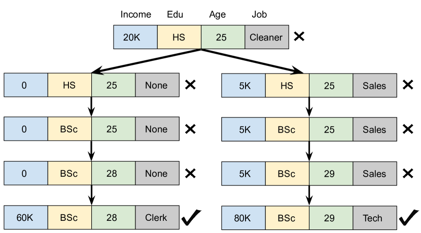
Figure 1: Example of Stochastic Algorithmic Recourses. Starting with a datapoint (✘ denotes undesired class prediction), FastAR can stochastically generate ARs that lead to different counterfactual states (✔ denotes desired class prediction).

In summary, our contributions are:

1. A novel algorithm that translates an AR problem into a Markov decision process (MDP). To the best of our knowledge, our stochastic-control-based approach is the first to address several roadblocks to using ARs in practice that have been identified by the community (Verma, Dickerson, and Hines 2020; Chou et al. 2021; Karimi et al. 2020b).

2. The first approach that generates sequential and amortized ARs, and also works for black-box models.

3. An extensive evaluation with three real-world datasets and nine baselines.

2 Desiderata of Practical ARs

The overarching goal of an AR is to provide practical guidance to an individual seeking to change their treatment (e.g., class label) by a deployed ML model. Apart from the necessary property of a AR having a desired class label, other desiderata have been identified in the literature, enumerated here:

• Actionability: ARs should only recommend changes to the features that are actionable (Ustun, Spangher, and Liu 2019; Kanamori et al. 2020; Dandl et al. 2020). Actionable features are dataset and preference dependent.

• Sparsity: Social studies have argued that smaller explanations are more comprehensible to humans (Miller 2019). Therefore ARs should make changes to a small set of features (Van Looveren and Klaise 2020; Karimi et al. 2020a).

• Data manifold: To obey the correlations between features, their input domain, and to be realistic, ARs should adhere to the training data manifold (Dhurandhar et al. 2019; Kanamori et al. 2020; Dandl et al. 2020).

• Causal constraints: In order to adhere to real-world constraints in ARs, causal constraints between features must be respected. They can encode facts like age cannot decrease or increase in education level increases age (Mahajan, Tan, and Sharma 2020).

• Model-agnostic: For wide-spread applicability, AR generating approaches should be model-agnostic (Laugel et al. 2018; Guidotti et al. 2018a).

• Black-box models: For applicability to proprietary ML models, AR generating approaches should work for black-box models (Sharma, Henderson, and Ghosh 2019).

• Amortized: An amortized approach can generate ARs for several datapoints without optimizing separately for each of them. Such an approach is effective for deployment (Mahajan, Tan, and Sharma 2020).

FastAR satisfies all the above desiderata. To the best of our knowledge, it is the first approach to do so (see Table 1). The choice of action space helps produce ARs that consider actionability among features and are sparse. It only modifies the actionable features. Its ARs are realistic as they adhere to the training data manifold and respect causal relations between features. FastAR works for black-box models and, therefore, is model-agnostic. It learns a policy that can produce ARs for several input datapoints without the need to optimize again; and, therefore, generates amortized ARs.

Table 1: Desiderata comparison of various AR generating approaches. FastAR is the first and only one which satisfies all desiderata.

Approach	Actionability	Sparsity	Agnostic	Black-box	Amortized	Manifold	Constraints
CFE Expl. (Wachter, Mittelstadt, and Russell 2017)	✗	✓	✗	✗	✗	✗	✗
Recourse (Ustun, Spangher, and Liu 2019)	✓	✓	✗	✗	✗	✗	✗
CEM (Dhurandhar et al. 2019)	✗	✓	✗	✗	✗	✓	✗
MACE (Karimi et al. 2020a)	✓	✓	✗	✗	✗	✗	✗
DACE (Kanamori et al. 2020)	✓	✗	✗	✗	✗	✓	✗
DiCE (Mothilal, Sharma, and Tan 2020)	✓	✓	✗	✗	✗	✗	✗
DiCE VAE (Mahajan, Tan, and Sharma 2020)	✓	✗	✗	✗	✓	✓	✓
Spheres (Laugel et al. 2018)	✗	✓	✓	✓	✗	✗	✗
LORE (Guidotti et al. 2018a)	✗	✓	✓	✓	✗	✗	✗
Weighted (Grath et al. 2018)	✗	✗	✓	✓	✗	✗	✗
CERTIFAI (Sharma, Henderson, and Ghosh 2019)	✓	✗	✓	✓	✗	✗	✗
Prototypes (Van Looveren and Klaise 2020)	✗	✓	✓	✓	✗	✓	✗
MOC (Dandl et al. 2020)	✓	✓	✓	✓	✗	✓	✗
FastAR	✓	✓	✓	✓	✓	✓	✓

3 Examples of Translating ARs to MDPs

We now give two examples of translating an AR problem into an MDP. Once modeled as an MDP, we can use various off-the-shelf algorithms (from planning or RL) to learn a policy to generate ARs.

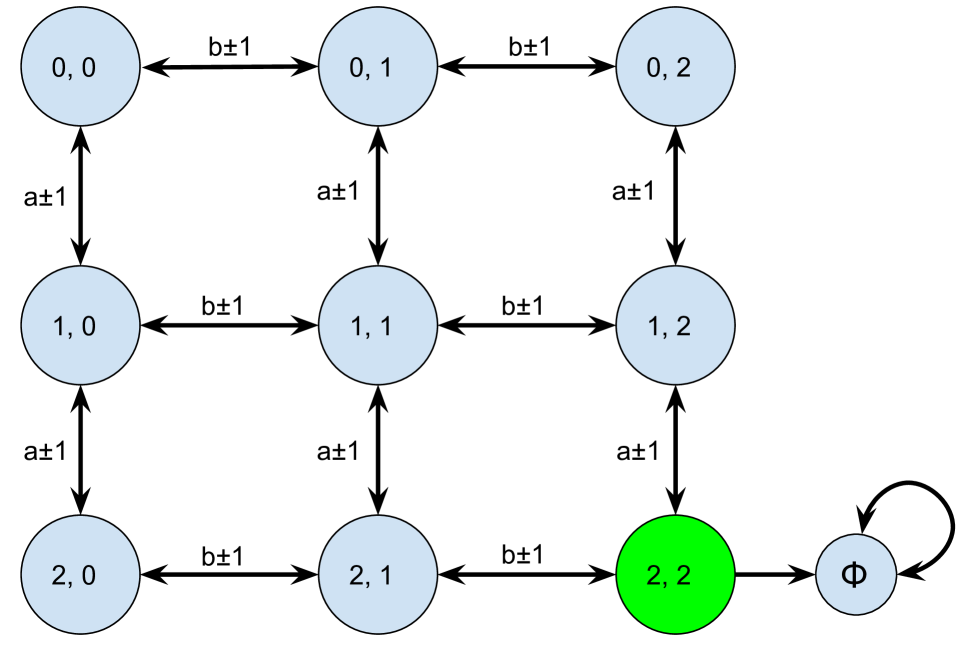
(a)

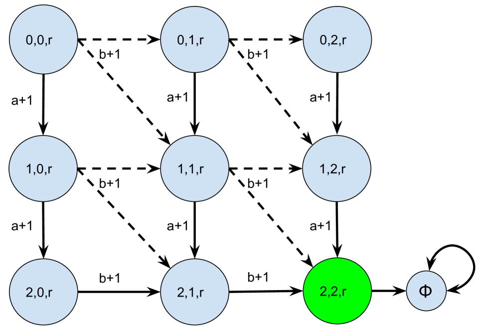
(b)

Figure 2: Transition function for the two examples. Circles show all the states, and edges show possible transitions. 1) Left-hand-side shows the transition function for a dataset with two features a and b, with no restrictions on the values both of them can take within the input domain. The transition edges are therefore bidirectional. 2) Right-hand-side shows the transition function for a dataset with three features: age (a), education-level (b), and race (r). The transition edges are unidirectional as both age and education cannot decrease. Since race is immutable, there are no actions for r. Since an increase in education stochastically affects age, the dashed edges represent a 50% probability of transition.

Example 1: Consider two categorical features $\textsf{a},\textsf{b}\in\{0,1,2\}$. The combinations of possible values for a and b form the state space for the MDP (represented by $\mathcal{S}$). The directed edges in Figure 2(a) show that upon taking a specific action, an agent can move from one state to another, e.g., it transits from state (0, 1) to (0, 2) by taking the action b+1, which increments the value of feature b by 1. Actions a+1 and a-1 respectively increase and decrease the value of feature a by 1 (similarly for feature b. These actions constitute the action space for the MDP (represented by $\mathcal{A}$). The third component of the MDP is the transition function which is represented by $\mathit{T:s\times a\to s^{\prime}}$. This denotes that if an agent takes action $a$ in state $s$ then it will move to state $s^{\prime}$. This transition function is deterministic because taking the action $a$ in state $s$ will always land the agent in the state $s^{\prime}$.

The final component of the MDP is the reward function. Taking action costs something (negative reward), and reaching desirable states generate a positive reward. In this MDP taking any action costs a constant amount of 1 and reaching the terminal state ($\phi$) gives a reward of +10. The terminal state ($\phi$) can only be reached via (2,2) (using any action), the state in green color. All actions in the terminal state lead to itself with 0 cost. This represents the situation in which a ML model classifies only (2,2) in the desired class.

The aim is to learn a policy that reaches a terminal state from any state at the lowest cost (e.g., taking the fewest number of steps). Cost (or reward) can be discounted in the traditional way using a discount factor $\gamma\in[0,1)$. Formally, for this example with a discrete state space and discrete action space, our MDP is:

• States = $\{s\in\mathcal{S}:\{0,0\},\{0,1\},\{0,2\},\{1,0\},\dots\}$.

• Actions = $\{a\in\mathcal{A}:\textsf{a+1},\textsf{a-1},\textsf{b+1},\textsf{b-1}\}$.

• Transition function $\mathit{T:\mathcal{S}\times\mathcal{A}\rightarrow\mathcal{S}}$

• Reward function $r:\mathcal{S}\times\mathcal{A}\to\mathbb{R}$.

• Discount factor $\gamma\in[0,1)$, capturing the tradeoff between current and future reward.

Our goal is finding a policy $\pi:\mathcal{S}\to\mathcal{A}$ that, given a state $s\in\mathcal{S}$ (an input datapoint), returns an action $a\in\mathcal{A}$ that represents the best first step to take to reach a new state, hopefully closer to the ML model’s decision boundary. FastAR would then call this precomputed policy repeatedly to find an optimal path to a counterfactual state.

Example 2: Now, consider a more realistic dataset having 3 features: age (denoted by a), education-level (denoted by b), and race (denoted by r). This is accompanied by real-world constraints like age and education-level cannot decrease, education-level affects age, and race is immutable. When we increase the education-level (b) by 1, there is a 50% chance that age group (a) will remain the same and a 50% chance that it will increase by 1. These interactions between features can be captured by a structural causal model (SCM), as we discuss in Section 4. The transition function for the MDP representing the AR problem for this dataset is, therefore, stochastic.

Defined formally, here are the components for this MDP:

• States = $\{s\in\mathcal{S}:\{0,0,0\},\{0,1,0\},\{0,2,1\},\dots\}$.

• Actions = $\{a\in\mathcal{A}:\textsf{a+1},\textsf{a-1},\textsf{b+1},\textsf{b-1}\}$.

• Transition function $\mathit{T:\mathcal{S}\times\mathcal{A}\times\mathcal{S^{\prime}}\to}$ {0,1} s.t. $\forall s\in\mathcal{S},\forall a\in\mathcal{A},\ \ \sum_{s^{\prime}\in\mathcal{S}}T(S,A,S^{\prime})=1.$

• Reward function $r:\mathcal{S}\times\mathcal{A}\to\mathbb{R}$.

• Discount factor $\gamma\in[0,1)$.

Figure 2(b) shows the transition function for this problem. The action that increases the education-level (b) now has a probabilistic transition to two destination states, represented by dashed unidirectional edges. Each transition edge has a 50% probability of occurrence. Unidirectionality comes from the fact that education-level cannot decrease. The edges change feature a are also unidirectional as age cannot decrease. The reward function is identical to the previous example; optionally, it can be changed to accommodate adherence to the data manifold (Section 2) or having different costs for changing different features, which we describe in Section 4. Additional examples can be found in Appendix C.

4 An Algorithmic Approach for Generating MDPs from AR Problems

1

2

Input : Training Dataset (D), ML model (f), Structural Causal Model (SCM), Numerical actionable features (NumA), Categorical actionable feature (CatA), Data Manifold distance function (DistD), Data Manifold adherence ($\lambda$), Desired Label (L), Distance Function (DistF), Discount Factor ($\gamma$)

Output : MDP

3

4

5

6

// States consist of all numerical (Num) and categorical (Cat) features.

7 $\mathit{\text{State space }\mathcal{S}\subseteq\mathbb{R}^{|\textnormal{{{Num}}}|}\times\mathbb{Z}^{|\textnormal{{{Cat}}}|}}$

8

// Actions change the actionable numerical and categorical features.

9 $\mathit{\text{Action space }\mathcal{A}\subseteq\mathbb{R}^{|\textnormal{{{NumA}}}|}\times\mathbb{Z}^{|\textnormal{{{CatA}}}|};\text{denote actions }A\in\mathcal{A}}$

10

11Function $\mathit{\textnormal{{Reward}}(\textnormal{{f}},\textnormal{{L}},\textnormal{{{CurrState}}},\textnormal{{$A$}},\textnormal{{{D}}},\lambda,\textnormal{{{DistD}}},\textnormal{{{SCM}}})}$

12       $\mathit{\textnormal{{{NextState}}}\leftarrow\textnormal{{Transition}}(\textnormal{{{CurrState}}},\textnormal{{$A$}},\textnormal{{{SCM}}})}$

13       if $\mathit{\textnormal{{argmax}}(\textnormal{{f}}(\textnormal{{{NextState}}}))}=\textnormal{{L}}$ then

            $\mathit{\textnormal{{{CFReward}}}\leftarrow\textnormal{{{Pos}}}}$ // High positive reward

14            

15      else

            $\mathit{\textnormal{{{CFReward}}}\leftarrow\textnormal{{f}}(\textnormal{{{NextState}}})[\textnormal{{L}}]}$ // Probability of classification in the desired class

16            

      return $\textnormal{{{DistF}}}(\textnormal{{{CurrState}}},\textnormal{{$A$}},\textnormal{{{D}}})$ // action cost

       $+\lambda*\textnormal{{{DistD}}}(\textnormal{{{NextState}}},\textnormal{{{D}}})$ // Manifold distance cost

       $+\textnormal{{{CFReward}}}$ // Counterfactual label reward

17      

18Function $\mathit{\textnormal{{Transition}}(\textnormal{{{CurrState}}},\textnormal{{$A$}},\textnormal{{{SCM}}}})$

       // Action does not violate feature domain and unary constraints

19       if Allowed ($A$) & InDomain ($A$)  then

            $\mathit{\textnormal{{{NextState}}}\leftarrow\textnormal{{{CurrState}}}+\textnormal{{$A$}}}$ // Modify features

20            

21      else

22            return CurrState

      // Modify the endogenous features

23      

24      for $\mathit{\textnormal{{{V}}}\in\textnormal{{{SCM}}}}$  do

25             if $\mathit{\textnormal{{$A$}}\in\textnormal{{Parent}}(\textnormal{{{V}}})}$  then

                   $\mathit{\textnormal{{{NextState}}}[\textnormal{{{V}}}]\leftarrow\textnormal{{{F}}}(\textnormal{{{U}}})}$ // Stochastic or deterministic update of endogenous features

26                  

27            

28      return NextState

$\mathit{\textnormal{{{MDP}}}\leftarrow\{\mathcal{S},\mathcal{A},\textnormal{{Transition}},\textnormal{{Reward}},\gamma\}}$

Algorithm 1 Generate MDP from an Algorithmic Recourse Problem

We now present a general approach for translating an AR problem setup into an MDP. Algorithm 1 generates all components of an MDP: state space, action space, transition function, reward function, and additional parameters such as discount factor. We detail this process below.

State space. Features can be broadly categorized into numerical (Num) and categorical (Cat) kinds. Numerical features can take real number values within a specified domain, while categorical features are mapped to a set of integers. Consequently, the state space $\mathcal{S}$ of our MDP (algorithm 1) consists of the product of the continuous domains for numerical features (a subset of $\mathit{\mathbb{R}^{|\textsf{Num}|}}$) and product of the integer domains for categorical features (a subset of $\mathit{\mathbb{Z}^{|\textsf{Cat}|}}$).

Action space. To facilitate capturing actionability (Ustun, Spangher, and Liu 2019) and causal relationships between features (Karimi, Schölkopf, and Valera 2020), we further categorize features as follows:

• Actionable features can be directly changed by an individual, e.g., income, education level, age.

• Mutable but not actionable features are mutable but cannot be modified directly by an individual, e.g., credit score cannot be directly changed by a person, it changes due to change in features like income and credit history.

• Immutable features cannot change, e.g., race, birthplace.

The agent is permitted to change only the actionable numerical and categorical features (denoted by NumA and CatA). Consequently, the action space $\mathcal{A}$ is a subset of $\mathbb{R}^{|\textsf{NumA}|}\times\mathbb{Z}^{|\textsf{CatA}|}$ (algorithm 1). Categorical features are changed within their discrete domain, while numerical features are changed within their continuous domain. Algorithm 1 further enforces the infeasibility of out-of-domain actions.

Transition function. The transition function (algorithm 1) finds the modified state when an action is taken. This function is influenced by the structural causal model (SCM), which is an optional input to Algorithm 1. An SCM consists of a triplet M = $\langle\textsf{U},\textsf{V},\textsf{F}\rangle$. U is the set of exogenous features and V is the set of endogenous features. In terms of a causal graph, the exogenous features U consist of features that have no parents, i.e., they can change independently. The endogenous features V consists of features that have parents in U and/or other features in V. They change as an effect of change in their parents. F is the set of functions that determine the relationship between exogenous and endogenous features. They are termed as structural equations.

Since knowing the exact SCM is often infeasible, Mahajan, Tan, and Sharma (2020) overcome this limitation by utlizing constraints from domain knowledge. Algorithm 1 also accepts such contraints in unary (Un) and binary (Bin) forms. Even if this does not provide us with the precise functional form of the constraint, its nature can help the FastAR’s recourses to be realistic. Unary constraints are derived from the property of one feature, e.g., age and education level cannot decrease. Binary constraints are derived from the relation between two features, e.g., if the education level increases, age increases. If an action does not violate the domain of the feature it is changing, nor the constraints in the SCM, then the feature is modified in NextState (algorithm 1). If the modified feature is an exogenous feature, we update its children using the F functions (algorithm 1-1).

Note that if no SCM is input to the algorithm, that will allow transitions from any state to any state (with intermediate states), and FastAR would generate ARs using this unconstrained transition function.

Reward function. Algorithm 1 defines a reward function that, given a state and an action, returns a reward based on three components derived from the initial AR problem:

• Given the current state (CurrState), action ($A$), training dataset (D), and distance function DistF, the first part returns the appropriate cost to take that action (algorithm 1). The distance function can either be the $\ell_{p}$ norm of the change produced by the action or a more complex function.

• The second part adds a cost if a datapoint is far from the training data manifold (algorithm 1) (which is computed using the DistD function) A $\lambda$ factor is used to control the strictness of data manifold adherence.

• The third part rewards the agent with a large positive value if a counterfactual state is reached (CFReward in algorithm 1). To avoid sparse rewards, we partially reward the agent with a small reward equal to the probability of NextState being classified in the desired class (algorithm 1). However, the sparse rewards can only be used if the underlying ML model provides the class label probabilities instead of only the class label, e.g., a neural network or random forest.

Other parameters. MDPs require additional parameters such as the discount factor $\gamma\in[0,1]$. At a high level, setting $\gamma<1$ penalizes longer paths; for additional intuition, see Sutton and Barto (2018). We note that $\lambda$, DistD, and DistF are user-specified and domain-specific parameters that directly impact the reward function for the MDP. We instantiate them in the evaluation section (see section 5).

5 Evaluation

We provide experimental validation of FastAR using three real-world datasets and comparison using nine baselines. Our research questions (RQ) are motivated by the recourse desiderata discussed in Section 2, and are enumerated here:

RQ1

Does FastAR successfully generate ARs for various input datapoints (validity)?

RQ2

How much change is required to reach a counterfactual state (proximity)?

RQ3

How many features are changed to reach a counterfactual state (sparsity)?

RQ4

Do the generated ARs adhere to the data manifold (realisticness)?

RQ5

Do the generated ARs respect causal and feature immutability constraints (feasibility)?

RQ6

How much time does FastAR take to generate ARs (amortizability)?

Datasets.

Motivated by most previous AR generating approaches (Verma, Dickerson, and Hines 2020), we use three datasets in our experiments: German Credit, Adult Income, and Credit Default (Dua and Graff 2017). These datasets have 20, 13 (omitted education-num as it has one to one mapping with education), and 23 features respectively. We split the datasets into 80%-10%-10% for training, validation, and testing, respectively. Each dataset has two labels, ‘1’ and ‘0’, where ‘1’ is the desired label. We trained a simple classifier: a neural network with two hidden layers (5 and 3 neurons) with ReLU activations. The test accuracy of the classifier was 83.0% for German Credit, 83.7% for Adult Income, and 83.2% for Credit Default. Note that the classifier’s accuracy is relatively less important for FastAR’s validation.

Implementation Algorithm.

Any appropriate method for computing an optimal policy $\pi^{*}:\mathcal{S}\to\mathcal{A}$, or any approximately optimal policy, to the MDP output of Algorithm 1 can be used. Our MDPhas a continuous state and action space, and therefore we use a policy gradient algorithm. Specifically, we use proximal policy optimization (PPO) with generalized advantage estimate (GAE) (Schulman et al. 2017; Mnih et al. 2016; Schulman et al. 2018) to train the agent. We justify this choice and answer several other related questions in Appendix E. The features in all datasets are scaled between $-1$ and $1$ before training both the ML model and the RL agent.

5.1 Baselines

Since, to our knowledge, FastAR is the first approach to generate amortized ARs for black-box models, there exist no previous approaches which we can directly compare against. Nevertheless, we compare FastAR to several previous popular AR generating approaches.

Baselines we developed. To compare FastAR to approaches that generated ARs in an amortized manner for black-box models, we developed two baselines:

• Random: This approach tries to reach a counterfactual state by executing random actions from the action space.

• Greedy: At each step, this approach greedily chooses the action (among all actions) which gives the highest reward.

Previous AR generating approaches. Based on the level of required model access, AR generating approaches can be categorized as: 1) access to complete model internals, i.e., weights of neurons or nodes of decision trees, 2) access to model gradients (restricted to differentiable models like neural networks), and 3) access to only the predict function (black-box). We choose popular methods from all categories:

• Complete model internal access. We chose MACE (Karimi et al. 2020a) from this category.

• Gradients access. Here we chose DiCE-Gradient (Mothilal, Sharma, and Tan 2020) and DiCE-VAE (Mahajan, Tan, and Sharma 2020). Notably, DiCE-VAE is the only other amortized AR generation method, however, it requires gradients and is restricted to differentiable models.

• Black-box. Open-source repository of the aforementioned DiCE method also had three black-box and model-agnostic approaches, namely: DiCE-Genetic, DiCE-KD-Tree, and DiCE-Random. We choose these three and Prototypes (Van Looveren and Klaise 2020) for this category. We did not compare with MOC (Dandl et al. 2020) as DiCE-Genetic it also a genetic algorithm based approach and has uses Python code.

5.2 Experimental Methodology

Table 2: Causal constraints and immutable features for the datasets. We assume FastAR is provided with them.

Dataset	Causal constraints	Immutable features
German Credit	Age and Job cannot decrease	Foreign worker, Number of liable people, Personal status, Purpose
Adult Income	Age and Education cannot decrease, increasing Education increases Age	Marital-status, Race, Native-country, Sex
Credit Default	Age and Education cannot decrease, increasing Education increases Age	Sex, Marital status

Here we describe the specific details of some approaches:

FastAR specifics.

As stated in Section 4, the recourses generated by FastAR are realistic if provided with the actionability of features and causal constraints. These constraints can be provided using the complete/partial SCM of the data generating process or using domain knowledge. We assume these constraints are provided to FastAR and are shown in Table 2. As described in Algorithm 1, this directly impacts the transition function. We use a particular instantiation of Algorithm 1 in the experiments:

• Action space: To produce sequential ARs, actions modify only one feature at a time. However, endogenous features may simultaneously change due to change in their parent.

• Cost of action: We treat DistF function as a hyperparameter and use several values for it in the experiments.

• Data manifold distance: Following previous work (Dandl et al. 2020; Kanamori et al. 2020), we train $k$-Nearest Neighbor (KNN) algorithm on the training dataset and use it to find the $\ell_{1}$ distance of a given datapoint from its nearest neighbor ($k=1$) in the dataset (DistD). We use several values of the adherence factor $\lambda$ in the experiments.

• Counterfactual state reward (CFReward): The agent receives a reward equal to the probability of its state belonging to the desired class (this ranges between 0 and 1). However, when a counterfactual state is reached, the agent is rewarded with 100 points.

• Discount Factor: We use a discount factor $\gamma=0.99$. This value encourages the agent to learn a policy that takes a few steps to reach a counterfactual state.

We explore the impact of $\lambda$ hyperparameter in LABEL:sec:hyperparam, and give more implementation details in LABEL:sec:implementation-details.

MACE specifics.

MACE requires as input the type of ML classifier to be used. We could not use a neural network because of the MACE’s long runtime (see section 5.3), and and therefore choose logistic regression (LR) and random forest (RF), which had a reasonable runtime.

All approaches are requested to generate ARs for the test datapoints that are predicted as ‘0’ by the classifier. Due to the small size of the German Credit dataset, we generate ARs for datapoints that are predicted as ‘0’ both in the training and test sets. Thus we request ARs for 257 datapoints in the German credit, 7229 datapoints in the Adult Income, and 5363 datapoints in the Credit Default datasets. Since MACE uses a different classifier, the number of datapoints predicted as ‘0’ were slightly different. More details are provided in section 5.3. FastAR, random, and greedy approaches stop when they reach a counterfactual state (predicted as ‘1’) or exhaust 50 actions. Other baselines have no such timeout.

5.3 Results

Table 3: Comparison of FastAR to all baselines for various AR evaluation metrics. Validity is the percentage an AR is actually classified in the desired class. Prox-Num and Prox-Cat refers to the L1 distance of the datapoint and its AR for the numerical and categorical features respectively. Sparsity is the number of features that were changed to produce the AR. Manifold dist. is the distance of the AR as returned by the trained kNN algorithm. Constraints refer to the causal constraints adherence by the generated AR. Time is the average time to generate ARs. For Validity and Constraints, a higher value is better, and for all other columns, a lower value is better. MACE and DiCE-Gradient could not be run for larger datasets owing to their large computation time.

Dataset	Approach	#DataPts.	Validity	Prox-Num	Prox-Cat	Sparsity	Manifold dist.	Constraints	Time (s)
German Credit	Random	257	23.7	0.17	0.57	11.33	1.08	41.0	0.31
	Greedy	257	49.8	0.07	0.087	1.81	0.48	100.0	4.59
	DiCE-Genetic	257	98.1	0.67	0.26	6.52	2.39	45.6	1.71
	DiCE-KDTree	257	0.0	N/A	N/A	N/A	N/A	N/A	0.17
	DiCE-Random	257	100.0	0.33	0.10	1.93	2.40	93.4	0.17
	Prorotypes	207	100.0	0.26	0.58	13.1	1.0	5.3	25.9
	DiCE-Gradient	257	100.0	0.27	0.29	6.33	2.19	82.9	7.10
	DiCE-VAE	257	77.8	0.80	0.42	10.12	0.97	5.0	0.15
	MACE (LR)	210	100.0	0.36	0.017	1.99	0.60	97.1	38.45
	MACE (RF)	287	100.0	0.22	0.02	2.64	0.38	74.2	101.29
	FastAR	257	97.3	0.10	0.063	1.22	0.72	100.0	0.07
Adult Income	Random	7229	80.9	0.56	0.77	10.07	1.00	29.0	0.25
	Greedy	7229	97.7	0.04	0.02	1.18	0.17	95.0	0.27
	DiCE-Genetic	7229	89.5	0.71	0.27	4.43	0.46	23.0	3.43
	DiCE-KDTree	7229	0.0	N/A	N/A	N/A	N/A	N/A	0.59
	DiCE-Random	7229	100.0	0.82	0.04	1.64	1.24	90.0	0.22
	Prototypes	500	100.0	0.29	0.57	9.0	0.68	22.8	28.9
	DiCE-Gradient	500	84.0	0.18	0.012	2.78	0.51	82.4	59.75
	DiCE-VAE	7229	77.1	0.75	0.65	9.99	0.30	0.13	0.12
	FastAR	7229	100.0	0.04	0.0	1.00	0.18	100.0	0.015
Credit Default	Random	5363	12.8	4.85	0.68	14.54	1.30	41.5	0.63
	Greedy	5363	65.1	0.15	0.072	1.25	0.22	99.9	4.67
	DiCE-Genetic	5363	92.6	3.93	0.49	16.67	2.75	27.9	3.58
	DiCE-KDTree	5363	0.0	N/A	N/A	N/A	N/A	N/A	0.45
	DiCE-Random	5363	100.0	5.80	0.20	2.33	3.09	97.7	0.39
	Prototypes	500	100.0	4.9	0.86	21.0	1.24	0.0	27.3
	DiCE-Gradient	100	81.0	0.77	0.40	15.98	1.35	85.2	479.17
	DiCE-VAE	5363	76.4	1.6	0.68	20.1	0.31	8.9	0.18
	FastAR	5363	99.9	0.01	0.11	1.008	0.32	100.0	0.051

Table 3 shows the performance of FastAR and all the baselines on the recourse desiderata. We report the average validity, average proximity (separately for the numerical and categorical features), average sparsity, average data manifold distance, average causal constraints adherence, and the average time to generate the ARs per datapoint.

Answer to RQ1: As shown in Table 3, FastAR has very high validity for all datasets. For Adult Income, FastAR gets the highest validity at 100%, while for Credit Default and German Credit, it achieves the second and third highest validity, respectively. Random and greedy approaches have low validity in general. DiCE-Genetic has validity in the high range, but this comes at the cost of proximity, sparsity, and data manifold distance. DiCE-KDTree is unable to generate AR even for a single datapoint in all three datasets. DiCE-Random achieves 100% validity for all datasets, and just like DiCE-Genetic, this comes at the cost of proximity, sparsity, and data manifold distance. The conclusion is similar for DiCE-Gradient’s and Prototypes’ validity. DiCE-VAE’s validity is lower than 80% for all datasets. MACE also achieves 100% validity but is very expensive to run. Due to this, it was impractical to run MACE for the larger datasets, Adult Income and Credit Default (we show MACE run only for the German Credit dataset). MACE was even more expensive when the underlying classifier was a neural network, and we had to abandon that experiment. For the classifiers used for MACE, ‘0’ was predicted for 210 datapoints by logistic regression (LR) and 287 datapoints by random forest (RF). MACE was supposed to generate ARs for these datapoints.

Answer to RQ2: We measure proximity for numerical and categorical features separately (Prox-Num and Prox-Cat, respectively). For numerical features, the distance is the sum of the $\ell_{1}$ norm respectively divided by the median average deviation for each numerical feature. For categorical features, the distance is the number of categorical features changed divided by the total number of categorical features. These metrics were proposed and used in previous works (Mahajan, Tan, and Sharma 2020). FastAR’s ARs are most proximal for Adult Income and Credit Default datasets, and second best for German Credit. The random approach, Prototypes, and the five variants of DiCE have large proximity values. The greedy approach performs well on this metric, but its validity is very low. MACE’s performance is about average.

Answer to RQ3: FastAR achieves the lowest sparsity among all approaches. Following previous works (Mothilal, Sharma, and Tan 2020), we measure sparsity at the start and endpoint of a recourse. Random, Prototypes, DiCE-VAE, DiCE-Genetic, and DiCE-Gradient’s performance is abysmal. This is surprising because DiCE-Gradient has a post-hoc step specifically for reducing sparsity. Greedy, MACE, and DiCE-Random’s performance is about average.

Answer to RQ4: FastAR achieves low average manifold distance. It performs second best for Adult Income and Credit Default and is in the middle for German Credit. The greedy approach, MACE, and DiCE-VAE also perform well on this metric. The random approach, Prototypes, and all variants of DiCE (except DiCE-VAE) perform poorly on this metric.

Answer to RQ5: By construction, FastAR always respects causal constraints encoded in its transition function: it has 100% adherence in all datasets. The DiCE based approaches (except DiCE-VAE), MACE, and random approach take as input the immutable features, but not the other causal constraints and hence do not perform well. DiCE-VAE and Prototypes do not accept immutable features and hence perform the worst for this metric. The greedy approach performs well on this metric, even though it does not have a knowledge of the causal constraints.

Answer to RQ6: The final column in Table 3 reports the average computation time per AR. Owing to amortization, FastAR can generate ARs very quickly and takes the lowest time among all approaches. The next best performers are DiCE-VAE and DICE-Random. FastAR is 2$\times$ faster than DiCE-VAE on average (up to 8$\times$ faster), 8$\times$ faster than DiCE-random on average (up to 15$\times$ faster). DiCE-random and random approach perform similarly. The difference even more staggering for DiCE-Genetic, Prototypes, and greedy approach. MACE and Dice-Gradient were the slowest. FastAR is about 1000$\times$ faster than MACE on average (up to 1447$\times$ faster) and 4500$\times$ faster than DiCE-Gradient on average (up to 9400$\times$ faster). While amortization allows for the rapid generation of new ARs, there exists a one-time training cost. We give details about it in LABEL:sec:implementation-details.

6 Conclusion

We propose a novel RL-based approach, FastAR, that generates amortized and sequential recourses for black-box ML models. To the best of our knowledge, we are the first to propose such an approach. The ARs generated by FastAR possess desirable properties and when evaluated on the recourse metrics, they perform better than several popular baselines.

Appendix A Background

This section provides background about the social implications of ML models and techniques to address concerns, along with a brief introduction to Reinforcement Learning.

A.1 Fairness, Accountability, and Transparency of AI and ML

Fairness and explainability of an ML model are two major themes in the broad area of equitable ML learning research.

Fairness research mostly proposes algorithms that learn a model that does not discriminate against individuals belonging to disadvantaged demographic groups. Other possibilities of intervention lie in modifying the training data itself. Demographic groups are determined by values of sensitive attributes prescribed by law, e.g., race, sex, religion, or the nation of origin. ML models can get biased against certain demographic groups because of the bias in their training data, specifically label bias and selection bias. Label bias occurs due to manual biased labeling of datapoints belonging to a demographic group, e.g., if individuals from the black community were denied loans in the past irrespective of their ability to pay back, this gets captured in the data from which the model can learn. Selection bias occurs when specific subsets of a demographic group are selected, which captures potentially correlations between the prediction target and a specific demographic group, e.g., selecting only defaulters from a demographic group in the training data. More than 20 definitions of fairness of an ML model have been proposed in literature (Verma and Rubin 2018). Dunkelau and Leuschel (2019) summarize some of the significant research advances that have been made in fairness research, and is a comprehensive introductory text for understanding the categorization and direction of research.

Explainability research can be broadly divided into model explanation and outcome explanation research problems (Guidotti et al. 2018b). The model explanation problem seeks to search for an inherently interpretable and transparent model with high fidelity to the original complex model. Linear models, decision trees, and rule sets are examples of inherently interpretable models. There exists techniques to explain complex models like neural networks and tree ensembles using interpretable surrogate like decision tree (Craven and Shavlik 1995; Krishnan, Sivakumar, and Bhattacharya 1999; Chipman, George, and Mcculloch 1998; Domingos 1998) and rule sets (Deng 2014; Andrews, Diederich, and Tickle 1995). There also exist approaches that can be applied to black-box models (Henelius et al. 2014; Krishnan and Wu 2017; Zien et al. 2009).

The outcome explanation problem seeks to find, for a single datapoint and prediction from a model, an explanation of why the model made its prediction. The explanation is either provided in the form of the importance of each feature in the datapoint, or the form of example datapoints. The first class of methods are called feature attribution methods and are grouped into model-specific (Zhou et al. 2016; Selvaraju et al. 2017) and model-agnostic (Poulin et al. 2006; Ribeiro, Singh, and Guestrin 2016; Turner 2016) kinds. Example-based approaches return a few datapoints that either have the same class label as the original datapoint or a different class label. The motivation for the first is to provide a set of datapoints that must be similar in the input space. The motivation for the second is to provide a set of datapoints that serves as a target to achieve in case the individual wants to receive the alternative label. The second set of datapoints can be referred to as counterfactual explanations.

Counterfactual explanations are applicable to supervised machine learning where the desired label has not been obtained for a datapoint. Most research in counterfactual explanations assumes a classification setting. Supervised ML setup consists of several labeled datapoints, which are inputs to the algorithm, and the aim is to learn a function mapping from the input datapoints (with say m features) to labels. In classification, the labels are discrete values. The input space is denoted by $\mathcal{X}^{m}$ and the output space is denoted by $\mathcal{Y}$. The learned function is the mapping $f:\mathcal{X}^{m}\to\mathcal{Y}$ is used to make predictions. We expound on counterfactual explanations and their desirable properties in Section 2.

Major beneficiaries of explainable machine learning include the healthcare and finance sectors, which have a huge social impact (Tjoa and Guan 2019). We point the readers to surveys in the area of explainable machine learning (Adadi and Berrada 2018; Carvalho, Pereira, and Cardoso 2019; Guidotti et al. 2018b).

A.2 Reinforcement Learning

Reinforcement Learning (RL) is one of the three broad classes of machine learning, along with supervised and unsupervised learning. In RL, the goal is to explore a given environment and to learn a policy over time that dictates what action should be taken at a given state. The exploration happens with the help of an agent. Therefore, a policy is a mapping from a state to an action. When an action is taken at a state, the environment returns with the new state and a reward. A good policy aims to maximize the reward over time. The calculation of the new state is facilitated through the transition function, whereas the calculation of the reward is done using the reward function. Naturally, the agent can either learn policies that are greedy and only focus on immediate reward or learn policies that focus on reward in the long-term. This trade-off is controlled by a discount factor called $\gamma$, whose value lies between 0 and 1 (inclusive of 0 and 1). States can either be discrete or continuous. Similarly, actions can also be either discrete or continuous. An RL problem is expressed in terms of a Markov Decision Process (MDP), which has five components. We illustrate each of them using the game of chess.

• State space $\mathcal{S}$, which are states an agent might explore. In chess, these are the 64 squares that an agent can move to.

• Action space $\mathcal{A}$, which are the possible actions an agent can take. These might be restricted based on the current state. In chess, the actions depend on the game pieces like a king, queen or pawns, and the given position on the chessboard. The action space is the union of all possible actions.

• Transition function T which given the current state and action, find the new state that the agent will transition to, e.g., moving the pawn by 1 unit north end up putting the agent in the state that is one unit north of its current state. Transition functions can be deterministic or stochastic (see Section 3).

• Reward function R passes the reward to the agent given the action, the current state, and the new state. This reward signal is the main factor that the agent uses to learn a good policy, e.g., winning a game would pass a positive reward, and losing the game would send a negative reward to the agent.

• Discount factor $\gamma$ is associated with the nature of the problem at hand. This is used to decide the trade-off between immediate and long-term rewards.

Many algorithms have been developed to efficiently learn an agent, given the environment like value iteration, policy iteration, policy gradient, actor-critic methods (Sutton and Barto 2018).

Appendix B Related Works

Literature in counterfactual explanations for ML is relatively recent, with the first proposed algorithm in 2017. Wachter, Mittelstadt, and Russell (2017) proposed finding counterfactuals as a constrained optimization problem where the goal is to find the minimum change in the features such that the new datapoint has the desired label. This approach was gradient-based, did not consider actionability among features, did not adhere to data manifold or respect causal relations, and the optimization problem needed to be solved for generating a CFE for each input datapoint. Other desiderata mentioned in Section 2 were proposed by other papers: 1) approaches that generate multiple, diverse counterfactuals for a single input datapoint (Mothilal, Sharma, and Tan 2020; Dandl et al. 2020; Mahajan, Tan, and Sharma 2020; Karimi et al. 2020a; Sharma, Henderson, and Ghosh 2019; Russell 2019), 2) approaches that generate counterfactual for black-box models and are model-agnostic (Lash et al. 2017; Laugel et al. 2018; Guidotti et al. 2018a; Grath et al. 2018; Sharma, Henderson, and Ghosh 2019; Rathi 2019; White and Garcez 2019; Poyiadzi et al. 2020; Keane and Smyth 2020; Dandl et al. 2020), 3) approaches that generate CFEs adhering to data manifold (Dhurandhar et al. 2018, 2019; Joshi et al. 2019; Van Looveren and Klaise 2020; Mahajan, Tan, and Sharma 2020; Pawelczyk, Broelemann, and Kasneci 2020; Keane and Smyth 2020; Le, Wang, and Lee 2019; Dandl et al. 2020; Kanamori et al. 2020), 4) approaches that generate CFEs that respect causal relations (Mahajan, Tan, and Sharma 2020; Karimi, Schölkopf, and Valera 2020; Karimi et al. 2020c), 5) approaches that generate amortized CFEs (Mahajan, Tan, and Sharma 2020).

Mahajan, Tan, and Sharma (2020) was the first to propose an approach that can generate multiple CFEs for many datapoints, after optimizing once, therefore amortized CFEs, but their approach is gradient-based and therefore works only for differentiable models and it not black-box. Our approach overcomes this limitation and generates both amortized and model-agnostic CFEs, which adhere to data manifold and respect causal relations. Out of the previous approaches that respect causal relations, only Mahajan, Tan, and Sharma (2020) works with partial SCM, while others require complete causal graph or complete SCM (Karimi, Schölkopf, and Valera 2020; Karimi et al. 2020c), which are mostly unavailable in the real world. Our approach also works with a partial SCM.

All the previous works give a single-shot solution for getting to a counterfactual state from an input datapoint. Our approach overcomes this limitation by proposing a novel algorithm that generates sequential CFEs.

Verma, Dickerson, and Hines (2020) and Karimi et al. (2020b) have collected and summarized recent works in counterfactual explainability. We point the readers to these surveys for an excellent in-depth review of the research landscape in this area.

Appendix C Illustrative examples

This section gives the remaining examples of translating a CFE problem into an MDP.

Example 1: Let us now consider the example where one of the two features is age (denoted by feature a). This adds a constraint because age cannot decrease. This is captured by the transition function. In Figure 3 we see that the edges which act on feature a have now become unidirectional implying that the value of feature a cannot decrease, action a-1 is not allowed.

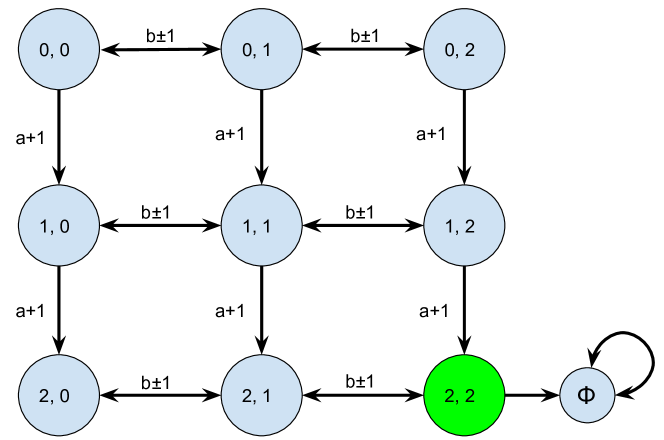
Figure 3: Transition function for a dataset with 2 features, out of which one is age (denoted by a). Circles show the states and edges show possible transitions. The edges which denote action on the feature a are unidirectional as age cannot decrease. Action a-1 taken at any state would loop back to the same state. Each action has a constant cost of 1.

Defined formally, here are the components for this MDP:

• States $\mathcal{S}$ = {0,0}, {0,1}, {0,2}, {1,0}, ….

• Actions $\mathcal{A}$ = a+1, b+1, b-1.

• Transition function $\mathit{T:\mathcal{S}\times\mathcal{A}\rightarrow\mathcal{S}}$

• Reward function $R:\mathcal{S}\times\mathcal{A}\to\mathbb{R}$.

• Discount factor $\gamma\in[0,1)$.

Example 2: Let us now consider a dataset with three features, out of which one is immutable, e.g., race (denoted by feature r). Feature a still represents age and carries its non-decreasing constraint. Such a feature cannot be changed using any action, and this is encoded in the transition function by returning the same state if this action is taken. The state space in this MDP will consist of 3 values, one for each feature. Figure 4 shows the transition function for the MDP representing the CFE problem using this dataset. As we already saw, a which represents age is non-decreasing. Also, none of the actions affect the value of feature r, it remains constant (shown by the constant ‘r’ in the diagram). The reward function is similar to the first example: a constant cost to take any action and a high reward for reaching the terminal state where the first two features are (2,2). This state follows into a dummy state where any action ends up in the same dummy state.

Figure 4: Transition function for a dataset with 3 features, the first being age (denoted by a) and the third being race (denoted by r). Circles show all the states and edges show possible transitions. None of the actions can change the value of feature r as race is immutable.

Let r take values 0 and 1.

Defined formally, here are the components for this MDP:

• States $\mathcal{S}$ = {0,0,0}, {0,1,0}, {0,2,1}, {1,0,0}, ….

• Actions $\mathcal{A}$ = a+1, b+1, b-1.

• Transition function $\mathit{T:\mathcal{S}\times\mathcal{A}\rightarrow\mathcal{S}}$

• Reward function $R:\mathcal{S}\times\mathcal{A}\to\mathbb{R}$.

• Discount factor $\gamma\in[0,1)$.

Example 3: In all the examples we visited, there was a constant cost to taking any action, and all states but one gave a 0 reward on reaching them. Consider the previous example where the dataset consisted of 3 features: age, education-level, and race. Some of the states do not appear in the training dataset used to train the classifier we are trying to generate CFEs for. Ideally, we would prefer to generate CFEs that are similar to existing data; otherwise, we might generate unrealistic and unactionable explanations. This is based on the assumption that training data is a good representation of the true distribution of features. Some of such states are:

• (0,2,0) and (0,2,1): intuitively this shows that it is unrealistic for an individual to be in the lowest age group (0) and have the highest education-level (1). This is true regardless of the person’s race.

• (2,0,1): it is improbable for someone belonging to the race encoded by value 1 to be in the highest age group and have the lowest possible education-level. Yet (2,0,0) is not an improbable state, and this might be due to the differences in education level across different races.

We encode this information in the MDP by modifying its reward function. If we take an action that ends up in an unrealistic state, it attracts a penalty of -5 points. The dummy state still carries the +10 reward, other states reward 0, and there is a constant cost of 1 to take any action. The agent learning in this environment would ideally learn to avoid the unrealistic states and take actions that go to the terminal state. In this situation, the agent can learn not to take a shorter path because it goes through an unrealistic state. We use a $k$-Nearest Neighbour algorithm to find the appropriate penalty for landing in any state in our experiments. If a state is close to a datapoint in the training dataset or occurs in the training dataset itself, there is a low or no penalty.

Example 4: Reconsider the last example in which there are three features. The reward function in the last example costed the same for all features. It might be harder to change one feature than another in real life, e.g., it might be easier for someone to wait to increase their age rather than get a higher educational level. This can be accounted for by posting higher costs to change features harder to change and vice-versa for feature easier to change.

Appendix D Counterfactual vs. Contrastive explanations

There is ongoing discussion on the exact definition of counterfactual explanation, with some researchers advocating to call it contrastive explanations. Dhurandhar and Shanmugam (2020) have captured the precise difference in a recent article. They mention that the counterfactual explanations as introduced by Wachter, Mittelstadt, and Russell (2017) are almost the same as contrastive explanations. These explanations seek to find the minimal changes to the input such that the prediction from the ML model changes. On the other hand, counterfactuals are a function of the datapoint, its prediction, the ML model, and the data generating process that created that datapoint. Pearl (2000) describes three steps for generating counterfactuals:

1. Abduction: This is the process of conditioning on the exogenous variables in the data generation process.

2. Intervention: This is the process of making a sparse change on a specific observable variable.

3. Prediction: This is the process of using the exogenous variables identified in the first step and propagating the intervention to generate the counterfactual.

We agree with this framing. Therefore, counterfactual explanations amount to much more perturbing the input datapoint—as in the case of contrastive explanations, which are tied to the data generating process. Indeed, it is our belief that our proposed framework captures these concerns, if data regarding causal interactions is available.

We take note of this distinction and therefore have adherence to causal relations as a desiderata of counterfactual explanations (Section 2). Structural Causal Models (SCM) consists of the exogenous and endogenous variables involved in the data generation process. FastAR takes as input the SCM (partial SCM is supported) of the dataset and takes it into consideration while generating CFEs. If the SCM is not provided, the explanations generated by FastAR are basically contrastive explanations.

Appendix E Justification of the Choice for our Implementation Algorithm.

In this section, using a set of questions and answers we attempt to justify our choice of the algorithm used by FastAR to generate CFEs.

Ques 1.

Why not use planning algorithms?

References

- Adadi and Berrada (2018) Adadi, A.; and Berrada, M. 2018. Peeking inside the black-box: A survey on Explainable Artificial Intelligence (XAI). IEEE Access, PP.
- Andrews, Diederich, and Tickle (1995) Andrews, R.; Diederich, J.; and Tickle, A. B. 1995. Survey and Critique of Techniques for Extracting Rules from Trained Artificial Neural Networks. Know.-Based Syst., 8.
- Brockman et al. (2016) Brockman, G.; Cheung, V.; Pettersson, L.; Schneider, J.; Schulman, J.; Tang, J.; and Zaremba, W. 2016. OpenAI Gym. arXiv:arXiv:1606.01540.
- Carvalho, Pereira, and Cardoso (2019) Carvalho, D. V.; Pereira, E. M.; and Cardoso, J. S. 2019. Machine learning interpretability: A survey on methods and metrics. Electronics, 8.
- Chipman, George, and Mcculloch (1998) Chipman, H. A.; George, E. I.; and Mcculloch, R. E. 1998. Making Sense of a Forest of Trees. In Proceedings of the 30th Symposium on the Interface.
- Chou et al. (2021) Chou, Y.-L.; Moreira, C.; Bruza, P.; Ouyang, C.; and Jorge, J. 2021. Counterfactuals and Causability in Explainable Artificial Intelligence: Theory, Algorithms, and Applications. arXiv preprint arXiv:2103.04244.
- Craven and Shavlik (1995) Craven, M. W.; and Shavlik, J. W. 1995. Extracting Tree-Structured Representations of Trained Networks. In Conference on Neural Information Processing Systems (NeurIPS). Cambridge, MA, USA: MIT Press.
- Dandl et al. (2020) Dandl, S.; Molnar, C.; Binder, M.; and Bischl, B. 2020. Multi-Objective Counterfactual Explanations. arXiv:2004.11165 [cs, stat].
- Deng (2014) Deng, H. 2014. Interpreting Tree Ensembles with inTrees. arXiv:1408.5456.
- Dhurandhar et al. (2018) Dhurandhar, A.; Chen, P.-Y.; Luss, R.; Tu, C.-C.; Ting, P.; Shanmugam, K.; and Das, P. 2018. Explanations Based on the Missing: Towards Contrastive Explanations with Pertinent Negatives. In Conference on Neural Information Processing Systems (NeurIPS).
- Dhurandhar et al. (2019) Dhurandhar, A.; Pedapati, T.; Balakrishnan, A.; Chen, P.-Y.; Shanmugam, K.; and Puri, R. 2019. Model Agnostic Contrastive Explanations for Structured Data. arXiv:1906.00117 [cs, stat].
- Dhurandhar and Shanmugam (2020) Dhurandhar, A.; and Shanmugam, K. 2020. Counterfactual vs Contrastive Explanations in Artificial Intelligence. https://towardsdatascience.com/counterfactual-vs-contrastive-explanations-in-artificial-intelligence-e67a9cfc7e4e. Accessed: 2021-05-15.
- Domingos (1998) Domingos, P. 1998. Knowledge Discovery Via Multiple Models. Intell. Data Anal., 2.
- Dua and Graff (2017) Dua, D.; and Graff, C. 2017. UCI Machine Learning Repository.
- Dunkelau and Leuschel (2019) Dunkelau, J.; and Leuschel, M. 2019. Fairness-Aware Machine Learning.
- Ehsan et al. (2021a) Ehsan, U.; Liao, Q. V.; Muller, M.; Riedl, M. O.; and Weisz, J. D. 2021a. Expanding Explainability: Towards Social Transparency in AI systems. In CHI.
- Ehsan et al. (2021b) Ehsan, U.; Wintersberger, P.; Liao, Q. V.; Mara, M.; Streit, M.; Wachter, S.; Riener, A.; and Riedl, M. O. 2021b. Operationalizing Human-Centered Perspectives in Explainable AI. In CHI.
- Faggella (2020) Faggella, D. 2020. Machine Learning for Medical Diagnostics – 4 Current Applications. https://emerj.com/ai-sector-overviews/machine-learning-medical-diagnostics-4-current-applications/. Accessed: 2020-10-15.
- Ghallab, Nau, and Traverso (2016) Ghallab, M.; Nau, D.; and Traverso, P. 2016. Automated Planning and Acting. USA: Cambridge University Press, 1st edition. ISBN 1107037271.
- Grath et al. (2018) Grath, R. M.; Costabello, L.; Van, C. L.; Sweeney, P.; Kamiab, F.; Shen, Z.; and Lecue, F. 2018. Interpretable Credit Application Predictions With Counterfactual Explanations. arXiv:1811.05245 [cs].
- Guidotti et al. (2018a) Guidotti, R.; Monreale, A.; Ruggieri, S.; Pedreschi, D.; Turini, F.; and Giannotti, F. 2018a. Local Rule-Based Explanations of Black Box Decision Systems.
- Guidotti et al. (2018b) Guidotti, R.; Monreale, A.; Ruggieri, S.; Turini, F.; Giannotti, F.; and Pedreschi, D. 2018b. A Survey of Methods for Explaining Black Box Models. ACM Comput. Surv., 51.
- Henelius et al. (2014) Henelius, A.; Puolamäki, K.; Boström, H.; Asker, L.; and Papapetrou, P. 2014. A Peek into the Black Box: Exploring Classifiers by Randomization. Data Min. Knowl. Discov., 28.
- Holstein et al. (2019) Holstein, K.; Wortman Vaughan, J.; Daumé III, H.; Dudik, M.; and Wallach, H. 2019. Improving fairness in machine learning systems: What do industry practitioners need? In Conference on Human Factors in Computing Systems (CHI), 1–16.
- Joshi et al. (2019) Joshi, S.; Koyejo, O.; Vijitbenjaronk, W.; Kim, B.; and Ghosh, J. 2019. Towards Realistic Individual Recourse and Actionable Explanations in Black-Box Decision Making Systems.
- Kanamori et al. (2020) Kanamori, K.; Takagi, T.; Kobayashi, K.; and Arimura, H. 2020. DACE: Distribution-Aware Counterfactual Explanation by Mixed-Integer Linear Optimization. In International Joint Conference on Artificial Intelligence (IJCAI).
- Karimi et al. (2020a) Karimi, A.-H.; Barthe, G.; Balle, B.; and Valera, I. 2020a. Model-Agnostic Counterfactual Explanations for Consequential Decisions. In Proceedings of the 23rd International Conference on Artificial Intelligence and Statistics.
- Karimi et al. (2020b) Karimi, A.-H.; Barthe, G.; Schölkopf, B.; and Valera, I. 2020b. A survey of algorithmic recourse: definitions, formulations, solutions, and prospects. arXiv:2010.04050.
- Karimi, Schölkopf, and Valera (2020) Karimi, A.-H.; Schölkopf, B.; and Valera, I. 2020. Algorithmic Recourse: from Counterfactual Explanations to Interventions. arXiv:2002.06278 [cs, stat].
- Karimi et al. (2020c) Karimi, A.-H.; von Kügelgen, J.; Schölkopf, B.; and Valera, I. 2020c. Algorithmic recourse under imperfect causal knowledge: a probabilistic approach.
- Keane and Smyth (2020) Keane, M. T.; and Smyth, B. 2020. Good Counterfactuals and Where to Find Them: A Case-Based Technique for Generating Counterfactuals for Explainable AI (XAI). arXiv:2005.13997.
- Kostrikov (2018) Kostrikov, I. 2018. PyTorch Implementations of Reinforcement Learning Algorithms. https://github.com/ikostrikov/pytorch-a2c-ppo-acktr-gail.
- Krishnan, Sivakumar, and Bhattacharya (1999) Krishnan, R.; Sivakumar, G.; and Bhattacharya, P. 1999. Extracting decision trees from trained neural networks. Pattern Recognition, 32.
- Krishnan and Wu (2017) Krishnan, S.; and Wu, E. 2017. PALM: Machine Learning Explanations For Iterative Debugging. In Proceedings of the 2nd Workshop on Human-In-the-Loop Data Analytics.
- Lash et al. (2017) Lash, M. T.; Lin, Q.; Street, W. N.; Robinson, J. G.; and Ohlmann, J. W. 2017. Generalized Inverse Classification. In SDM.
- Laugel et al. (2018) Laugel, T.; Lesot, M.-J.; Marsala, C.; Renard, X.; and Detyniecki, M. 2018. Comparison-Based Inverse Classification for Interpretability in Machine Learning. In Information Processing and Management of Uncertainty in Knowledge-Based Systems, Theory and Foundations (IPMU). Springer International Publishing.
- Le, Wang, and Lee (2019) Le, T.; Wang, S.; and Lee, D. 2019. GRACE: Generating Concise and Informative Contrastive Sample to Explain Neural Network Model’s Prediction. arXiv:1911.02042.
- Liang et al. (2018) Liang, E.; Liaw, R.; Nishihara, R.; Moritz, P.; Fox, R.; Goldberg, K.; Gonzalez, J. E.; Jordan, M. I.; and Stoica, I. 2018. RLlib: Abstractions for Distributed Reinforcement Learning. In ICML.
- Liang et al. (2020) Liang, E.; Nishihara, R.; Liaw, R.; and et al. 2020. Ray. https://github.com/ray-project/ray.