Learning Stochastic Optimal Policies via Gradient Descent

Abstract

We systematically develop a learning-based treatment of stochastic optimal control (SOC), relying on direct optimization of parametric control policies. We propose a derivation of adjoint sensitivity results for stochastic differential equations through direct application of variational calculus. Then, given an objective function for a predetermined task specifying the desiderata for the controller, we optimize their parameters via iterative gradient descent methods. In doing so, we extend the range of applicability of classical SOC techniques, often requiring strict assumptions on the functional form of system and control. We verify the performance of the proposed approach on a continuous–time, finite horizon portfolio optimization with proportional transaction costs.

I Introduction

In this work we consider the following class of controlled stochastic dynamical systems:

$$\dot{x}_{t}=f(t,x_{t},u_{t})+g(t,x_{t},u_{t})\xi(t)$$ (1)

with state $x_{t}\in\mathbb{X}\subset\mathbb{R}^{n_{x}}$ and control policy $u_{t}\in\mathbb{U}\subset\mathbb{R}^{n_{u}}$. $\xi(t)\in\mathbb{R}^{n_{\xi}}$ is a stationary $\delta$-correlated Gaussian noise, i.e. $\forall t>0~{}~{}~{}\mathbb{E}[\xi(t)]=0$ and $\forall s,t$ such that $0<s<t$ it holds $\mathbb{E}[\xi(s)\xi(t)]={\delta}(s-t)$. The RHS of (1) comprises a drift term $f:\mathbb{R}\times\mathbb{X}\times\mathbb{U}\rightarrow\mathbb{R}^{{n_{x}}}$ and a diffusion term $g:\mathbb{R}\times\mathbb{X}\times\mathbb{U}\rightarrow\mathbb{R}^{{n_{x}}\times{n_{\xi}}}$. This paper develops a novel, systematic approach to learning optimal control policies for systems in the form (1), with respect to smooth scalar objective functions.

The link between stochastic optimal control (SOC) and learning has been explored in the discrete–time case [1] with policy iteration and value function approximation methods [2, 3] seeing widespread utilization in reinforcement learning [4]. Adaptive stochastic control has obtained explicit solutions through strict assumptions on the class of systems and objectives [5], preventing its applicability to the general case. Forward–backward SDEs (FBSDEs) have been also proposed to solve classic SOC problems [6], even employing neural approximators for value function dynamics [7, 8]. A further connection between SOC and machine learning has also been discussed within the continuous–depth paradigm of neural networks [9, 10, 11, 12]. [13] e.g. showed that fully connected residual networks converge, in the infinite depth and width limit, to diffusion processes.

A different class of techniques for SOC involves the analytic [14] or approximate solution [15] of Hamilton–Jacobi–Bellman (HJB) optimality conditions. These approaches either restrict the class of objectives functions to preserve analytic tractability, or develop specific approximate methods which generally become intractable in high–dimensions.

Here, we explore a different direction, motivated by the affinity between neural network training and optimal control which involve the reliance on carefully crafted objective functions encoding task–dependent desiderata.

In essence, the raison d’être of synthesizing optimal stochastic controllers through gradient–based techniques is to enrich the class of objectives for which an optimal controller can be found, as well scale the tractability to high-dimensional regimes. This is in line with the empirical results of modern machine learning research where large deep neural networks are often optimized on high–dimensional non–convex problems with outstanding performance [16, 17]. Gradient–based methods are also being explored in classic control settings to obtain a rigorous characterization of optimal control problems in the linear–quadratic regime [18, 19].

Notation

Let $(\Omega,\mathcal{F},P)$ be a probability space. If a property (event) $A\in\mathcal{F}$ holds with $P(A)=1$, we say that such property holds almost surely. A family of $\mathbb{X}$–valued random variables defined on a compact time domain $\mathbb{T}\subset\mathbb{R}$ $\{x_{t}\}_{t\in\mathbb{T}}$ is called stochastic process and is measurable if $x_{t}(A)$ is measurable with respect to the $\sigma$-algebra $\mathcal{B}(\mathbb{T})\times\mathcal{F}$ being $\mathcal{B}(\mathbb{T})$ the Borel-algebra of $\mathbb{T}$. As a convention, we use $\int_{s}^{t}=-\int_{t}^{s}$ if $s<t$ and we denote with $\delta$ the Krocnecker delta function.

II Stochastic Differential Equations

Although (1) “looks like a differential equation, it is really a meaningless string of symbols” [20]. This relation should be hence treated only as a pre–equation and cannot be studied in this form. Such ill–posedness arises from the fact that, being $\xi{(t)}$ a $\delta$–autocorrelated process, the noise fluctuates an infinite number of times with infinite variance in any time interval. Therefore, a rigorous treatment of the model requires a different calculus to consistently interpret the integration of the RHS of (1). The resulting well-defined version of (1) is known as a Stochastic Differential Equation (SDE) [21].

II-A Itô–Stratonovich Dilemma

According to Van Kampen [20], $\xi(t)$ might be thought as a random sequence of $\delta$ functions causing, at each time $t$, a sudden jump of $x_{t}$. The controversies on the interpretation of (1) arises over the fact that it does not specify which value of $x$ should be used to compute $g$ when the $\delta$ functions are applied. There exist two main interpretations of the issue, namely Itô’s [22] and Stratonovich’s [23]. Itô prescribes that $g$ should be computed with the value of $x$ before the jump while Stratonovich uses the mean value of $x$ before and after the jump. This choice leads to two different (yet, both admissible and equivalent) types of integration. Formally, consider a compact time horizon $\mathbb{T}=[0,T],~{}T>0$ and let $\{B_{t}\}_{t\in\mathbb{T}}$ be the standard ${n_{\xi}}$-dimensional Wiener process defined on a filtered probability space $(\Omega,\mathcal{F},P;\{\mathcal{F}_{t}\}_{t\in\mathbb{T}})$ which is such that $B_{0}=0$, $B_{t}$ is almost surely continuous in $t$, nowhere differentiable, has independent Gaussian increments, namely $\forall s,t\in\mathbb{T}~{}s<t\Rightarrow B_{t}-B_{s}\sim\mathcal{N}(0,t-s)$ and, for all $t\in\mathbb{T}$, we have $\xi(t)\differential t=\differential B_{t}$. Moreover, let $\phi_{t}:=g(t,x_{t},u_{t})$. Itô and Stratonovich integral calculi are then defined as $\int_{0}^{T}\phi_{t}\differential B_{t}=\lim_{|D|\rightarrow 0}\sum_{k=1}^{K}\phi_{t_{k-1}}(B_{t_{k}}-B_{t_{k-1}})$ and $\int_{0}^{T}\phi_{t}{\color[rgb]{0.3,0.3,1}\circ}\differential B_{t}=\lim_{|D|\rightarrow 0}\frac{1}{2}\sum_{k=1}^{K}\left(\phi_{t_{k}}-\phi_{t_{k-1}}\right)(B_{t_{k}}-B_{t_{k-1}})$, respectively, where $D$ is a given partition of $\mathbb{T}$, $D:=\{t_{k}:0=t_{0}<t_{1}<\cdots<t_{K}=T\}$, $|D|=\max_{k}(t_{k}-t_{k-1})$ and the limit is intended in the mean–square sense, (see [24]) if exists. Note that the symbol “$\circ$” in $\circ\differential B_{t}$ is used only to indicate that the integral is interpreted in the Stratonovich sense and does not stand for function composition. In the Stratonovich convention, we may use the standard rules of calculus while this is not the case for Itô’s. This is because Stratonovich calculus corresponds to the limit case of a smooth process with a small finite auto–correlation approaching $B_{t}$ [25]. Therefore, there are two different interpretations of (1): $\differential x_{t}=f(t,x_{t},u_{t})\differential t+g(t,x_{t},u_{t})\differential B_{t}$ and $\differential x_{t}=f(t,x_{t},u_{t})\differential t+g(t,x_{t},u_{t})\circ\differential B_{t}$. Despite their name, SDEs are formally defined as integral equations due to the non-differentiability of the Brownian paths $B_{t}$.

From a control systems perspective, on one hand Stratonovich interpretation seems more appealing for noisy physical systems as it captures the limiting case of multiplicative noise processes with a very small finite auto–correlation, often a reasonable assumption in real applications. However, if we need to treat diffusion terms as intrisic components of the system’s dynamics or impose martingale assumptions on the solutions of the SDE, the Itô convention should be adopted. In particular, this is always the case of financial applications, where stochastic optimal control is widely applied (see e.g. [26]).

Within the scope of this paper, we will mainly adopt the Stratonovich convention for consistency of notation. Nonetheless, all results presented in this manuscript can be equivalently derived for the Itô case. Indeed an Itô SDE can be transformed into a Stratonovich one (and viceversa) by the equivalence relation between the two calculi: for all $t\in\mathbb{T}$ $\int_{0}^{t}\phi_{s}\circ\differential B_{s}=\int_{0}^{t}\phi_{s}\differential B_{s}+\frac{1}{2}\int_{0}^{t}\sum_{i=1}^{n_{\xi}}\frac{\partial\phi_{s}^{(i)}}{\partial x}\phi_{s}^{(i)}\differential s$.

II-B Stratonovich SDE

We will formally introduce Stratonovich SDEs following the treatment of Kunita [27, 24]. For $0\leq s\leq t\leq T$ we denote by $\mathcal{F}_{s,t}$ the smallest $\sigma$-algebra containing all null sets of $\mathcal{F}$ with respect to which, for all $v,w\in\mathbb{T}$ such that $s\leq v\leq w\leq t$, $B_{w}-B_{v}$ is measurable. $\{\mathcal{F}_{s,t}\}_{s\leq t;s,t\in\mathbb{T}}$ is called a two–sided filtration generated by the Wiener process and we set write $\mathcal{F}_{t}=\mathcal{F}_{0,t}$ for compactness. Then, $\{\mathcal{F}_{t}\}_{t\in\mathbb{T}}$ is itself a filtration with respect to which $B_{t}$ is $\mathcal{F}_{t}$–adapted. Further, we let $f,g$ to be bounded in $\mathbb{X}$, infinitely differentiable in $x$, continuously differentiable in $t$, uniformly continuous in $u$ and we assumme the controller $\{u_{t}\}_{t\in\mathbb{T}}$ to be a $\mathcal{F}_{t}$–adapted process. Given an initial condition $x_{0}\in\mathbb{X}$ assumed to be a $\mathcal{F}_{0}$ measurable random variable, we suppose that there exists a $\mathbb{X}$-valued continuous $\mathcal{F}_{t}$-adapted semi–martingale $\{x_{t}\}_{t\in\mathbb{T}}$ such that

$$x_{T}=x_{0}+\int_{0}^{T}f(t,x_{t},u_{t})\differential t+\int_{0}^{T}g(t,x_{t},u_{t})\circ\differential B_{t},$$ (2)

almost surely. Path–wise existence and uniqueness of solutions, i.e. if, for all $t\in\mathbb{T}$, two solutions $x_{t},~{}x_{t}^{\prime}$ such that that $x_{0}=x_{0}^{\prime}$ satisfy $\forall t\in\mathbb{T}~{}x_{t}=x_{t}^{\prime}$ almost surely, is guaranteed under our class assumptions on $f,g$ and the process $\{u_{t}\}_{t\in\mathbb{T}}$.

If, as assumed here, $f$, $g$ are functions of class $\mathcal{C}^{1,\infty}$ in $(x_{t},t)$ uniformly continuous in $u$ with bounded derivatives w.r.t $x$ and $t$, and $\{u_{t}\}_{t\in\mathbb{T}}$ belongs to some admissible control set $\mathbb{A}$ of $\mathbb{T}\rightarrow\mathbb{U}$ functions, then, given a realization of the Wiener process, there exists a $\mathcal{C}^{\infty}$ mapping $\Phi$ called stochastic flow from $\mathbb{X}\times\mathbb{A}$ to the space of absolutely continuous functions $[s,t]\rightarrow\mathbb{X}$ such that

$$x_{t}=\Phi_{s}(x_{s},\{u_{s}\}_{s\leq t;s,t\in\mathbb{T}})(t)~{}~{}~{}s\leq t;s,t\in\mathbb{T};x_{s}\in\mathbb{X}$$ (3)

almost surely. For the sake of compactness we denote the RHS of (3) with $\Phi_{s,t}(x_{s})$. It is worth to be noticed that the collection $\{\Phi_{s,t}\}_{s\leq t;s,t\in\mathbb{T}}$ satisfies the flow property (see [24, Sec. 3.1]) $\forall s,t,v\in\mathbb{T}:s<v<t\Rightarrow\Phi_{v,t}(\Phi_{s,v}(x_{s}))=\Phi_{s,t}(x_{s})$ and that it is also a diffeomorphism [24, Theorem 3.7.1], i.e. there exists an inverse flow $\Psi_{s,t}:=\Phi^{-1}_{s,t}$ which satisfies the backward SDE

$$\Psi_{s,t}(x_{s})=x_{s}- \int_{s}^{t}f(v,\Psi_{s,v}(x_{s}),u_{v})\differential v$$

$$-\int_{s}^{t}g(v,\Psi_{s,v}(x_{s}),u_{v})\circ\differential{\mathchoice{{\ooalign{\hbox{\raise 7.09259pt\hbox{\scalebox{1.0}[-1.0]{\lower 7.09259pt\hbox{$\displaystyle\widehat{\vrule width=0.0pt,height=6.83331pt\vrule height=0.0pt,width=8.0868pt}$}}}}\cr\hbox{$\displaystyle B$}}}}{{\ooalign{\hbox{\raise 7.09259pt\hbox{\scalebox{1.0}[-1.0]{\lower 7.09259pt\hbox{$\textstyle\widehat{\vrule width=0.0pt,height=6.83331pt\vrule height=0.0pt,width=8.0868pt}$}}}}\cr\hbox{$\textstyle B$}}}}{{\ooalign{\hbox{\raise 6.40926pt\hbox{\scalebox{1.0}[-1.0]{\lower 6.40926pt\hbox{$\scriptstyle\widehat{\vrule width=0.0pt,height=4.78333pt\vrule height=0.0pt,width=5.66075pt}$}}}}\cr\hbox{$\scriptstyle B$}}}}{{\ooalign{\hbox{\raise 5.9537pt\hbox{\scalebox{1.0}[-1.0]{\lower 5.9537pt\hbox{$\scriptscriptstyle\widehat{\vrule width=0.0pt,height=3.41666pt\vrule height=0.0pt,width=4.0434pt}$}}}}\cr\hbox{$\scriptscriptstyle B$}}}}}_{v}.$$

being $\{{\mathchoice{{\ooalign{\hbox{\raise 7.09259pt\hbox{\scalebox{1.0}[-1.0]{\lower 7.09259pt\hbox{$\displaystyle\widehat{\vrule width=0.0pt,height=6.83331pt\vrule height=0.0pt,width=8.0868pt}$}}}}\cr\hbox{$\displaystyle B$}}}}{{\ooalign{\hbox{\raise 7.09259pt\hbox{\scalebox{1.0}[-1.0]{\lower 7.09259pt\hbox{$\textstyle\widehat{\vrule width=0.0pt,height=6.83331pt\vrule height=0.0pt,width=8.0868pt}$}}}}\cr\hbox{$\textstyle B$}}}}{{\ooalign{\hbox{\raise 6.40926pt\hbox{\scalebox{1.0}[-1.0]{\lower 6.40926pt\hbox{$\scriptstyle\widehat{\vrule width=0.0pt,height=4.78333pt\vrule height=0.0pt,width=5.66075pt}$}}}}\cr\hbox{$\scriptstyle B$}}}}{{\ooalign{\hbox{\raise 5.9537pt\hbox{\scalebox{1.0}[-1.0]{\lower 5.9537pt\hbox{$\scriptscriptstyle\widehat{\vrule width=0.0pt,height=3.41666pt\vrule height=0.0pt,width=4.0434pt}$}}}}\cr\hbox{$\scriptscriptstyle B$}}}}}_{t}\}_{t\in\mathbb{T}}$ the realization of the backward Wiener process defined as ${\mathchoice{{\ooalign{\hbox{\raise 7.09259pt\hbox{\scalebox{1.0}[-1.0]{\lower 7.09259pt\hbox{$\displaystyle\widehat{\vrule width=0.0pt,height=6.83331pt\vrule height=0.0pt,width=8.0868pt}$}}}}\cr\hbox{$\displaystyle B$}}}}{{\ooalign{\hbox{\raise 7.09259pt\hbox{\scalebox{1.0}[-1.0]{\lower 7.09259pt\hbox{$\textstyle\widehat{\vrule width=0.0pt,height=6.83331pt\vrule height=0.0pt,width=8.0868pt}$}}}}\cr\hbox{$\textstyle B$}}}}{{\ooalign{\hbox{\raise 6.40926pt\hbox{\scalebox{1.0}[-1.0]{\lower 6.40926pt\hbox{$\scriptstyle\widehat{\vrule width=0.0pt,height=4.78333pt\vrule height=0.0pt,width=5.66075pt}$}}}}\cr\hbox{$\scriptstyle B$}}}}{{\ooalign{\hbox{\raise 5.9537pt\hbox{\scalebox{1.0}[-1.0]{\lower 5.9537pt\hbox{$\scriptscriptstyle\widehat{\vrule width=0.0pt,height=3.41666pt\vrule height=0.0pt,width=4.0434pt}$}}}}\cr\hbox{$\scriptscriptstyle B$}}}}}_{t}:=B_{t}-B_{T}$ for all $t\in\mathbb{T}$. The diffeomorphism property of $\Phi_{s,t}$ thus yields: $\Psi_{s,t}(\Phi_{s,t}(x_{s}))=x_{s}$.

Therefore, it is possible to reverse the solutions of Stratonovich SDEs in a similar fashion to ordinary differential equations (ODEs) by storing/generating identical realizations of the noise process. From a practical point of view, under mild assumptions on the chosen numerical SDE scheme, approximated solutions $\hat{\Phi}_{s,t}(x_{s})$ satisfy $\forall x_{s}\in\mathbb{X}~{}~{}\hat{\Psi}_{s,t}(\hat{\Phi}_{s,t}(x_{s}))\rightarrow x_{s}$ in probability as the discretization time-step $\epsilon\rightarrow 0$ [28, Theorem 3.3].

III Direct Stochastic Optimal Control

We consider the optimal control problem for systems of class $\eqref{eq:1}$ interpreted in the Stratonovich sense. In particular, we aim at determining a control process $\{u_{t}\}_{t\in\mathbb{T}}$ within an admissible set of functions $\mathbb{A}$ to minimize or maximize in expectation some scalar criterion $J_{u}$ of the form

$$J_{u}(x_{0})=\int_{\mathbb{T}}\gamma(t,\Phi_{0,t}(x_{0}),u_{t})\differential t+\Gamma(\Phi_{0,T}(x_{0}),u_{T}),$$ (4)

measuring the performance of the system. Within the scope of the paper, we characterize $\mathbb{A}$ as set of all control processes $\{u_{r}\}_{t\in\mathbb{T}}$ which are $\mathcal{F}_{t}$–adapted, have values in $\mathbb{U}$ and such that $\mathbb{E}[\int_{\mathbb{T}}\|u_{t}\|_{2}^{2}]\differential t\leq\infty$. To emphasize the (implicit) dependence of $J_{u}(x_{0})$ on the realization of the Wiener process, we often explicitly write $J_{u}(x_{0},\{B_{t}\}_{t\in\mathbb{T}})$.

III-A Stochastic Gradient Descent

In this work we propose to directly seek the optimal controller via mini-batch stochastic gradient descent (SGD) (or ascent) optimization [29, 30]. The algorithm works as follows: given a scalar criterion $J_{\alpha}(x_{0},\{B_{t}\}_{t\in\mathbb{T}})$ dependent on the variable $\alpha$ and the Brownian path, it attempts at computing $\alpha^{*}=\arg\min_{\alpha}\mathbb{E}[J_{\alpha}(x_{0},\{B_{t}\}_{t\in\mathbb{T}})]$ or $\alpha^{*}=\arg\max_{\alpha}\mathbb{E}[J_{\alpha}(x_{0},\{B_{t}\}_{t\in\mathbb{T}})]$ starting from an initial guess $\alpha_{0}$ by updating a candidate solution $\alpha_{k}$ recursively as $\alpha_{k+1}=\alpha_{k}\pm\frac{\eta_{k}}{N}\sum_{i=1}^{N}\frac{\differential}{\differential\alpha}J_{\alpha_{k}}(x_{0},\{B_{t}\}_{t\in\mathbb{T}}^{i}),$ where $N$ is a predetermined number of independent and identically distributed samples $\{B_{t}\}_{t\in\mathbb{T}}^{i}$ of the Wiener process, $\eta_{k}$ is a positive scalar learning rate and the sign of the update depends on the minimization or maximization nature of the problem. If $\eta_{k}$ is suitably chosen and $J_{\alpha}$ is convex, $\alpha_{k}$ converges in expectation to the minimizer of $J_{\alpha}$ as $k\rightarrow\infty$. Although global convergence is no longer guaranteed in the non–convex case, SGD–based techniques have been employed across application areas due to their scaling and unique convergence characteristics. These methods have further been refined over time to show remarkable results even in non–convex settings [31, 32].

III-B Finite Dim. Optimization via Neural Approximators

Consider the case in which the criterion $J_{u}$ has to be minimized. Locally optimal control processes $u=\{u_{t}\}_{t\in\mathbb{T}}\in\mathbb{A}$ could be obtained, in principle, by iterating the SGD algorithm for the criterion $J_{u}$ in the set $\mathbb{A}$ of admissible control processes. Since $\mathbb{A}$ is at least in $L_{2}(\mathbb{T}\rightarrow\mathbb{U})$ we could preserve local convergence of SGD in the function-space [33]. An idealized function–space SGD algorithm would compute iterates of the form

$$u^{k+1}=u^{k}-\frac{\eta_{k}}{N}\sum\limits_{i=1}^{N}\dfrac{\delta}{\delta u}J_{u}(x_{s}0,\{B_{t}\}_{t\in\mathbb{T}}^{i})$$

where $u^{k}$ is the solution at the $k$th SGD iteration, $\delta/\delta(\cdot)$ is the variational or functional derivative and $J_{u}$ satisfies $\delta\mathbb{E}[J_{u}(x_{s},\{B_{t}\}_{t\in\mathbb{T}})]/\delta u=\mathbb{E}[\delta J_{u}(x_{s},\{B_{t}\}_{t\in\mathbb{T}})/\delta u]$.

At each training step of the controller, this approach would thus perform $N$ independent path simulations, compute the criterion $J_{u}$ and apply the gradient descent update. While local convergence to optimal solutions is still ensured under mild regularity and smoothness assumptions, obtaining derivatives in function space turns out to be computationally intractable. Any infinite-dimensional algorithm needs to be discretized in order to be practically implementable. We therefore seek to reduce the problem to finite dimension by approximating $u^{k}_{t}$ with a neural network.

Let $u_{\theta,t}:\theta,t\mapsto u_{\theta,t}$ be a neural network with parameters $\theta\in\mathbb{R}^{{n_{\theta}}}$ which we use as functional approximators for candidate optimal controllers, i.e. $u_{\theta,t}\approx u_{t}^{*}~{}\forall t\in\mathbb{T}$. Further, we denote $f_{\theta}(t,x_{t}):=f(t,x_{t},u_{\theta,t})$ and $g_{\theta}(t,x_{t}):=g(t,x_{t},u_{\theta,t})$ and the optimization criterion

$$J_{\theta}(x_{0})=\int_{\mathbb{T}}\gamma_{\theta}(t,\Phi_{s,t}(x_{0}))\differential t+\Gamma_{\theta}(T,\Phi_{s,T}(x_{0}))$$ (5)

with $\gamma_{\theta}(\cdot,\cdot)=\gamma(\cdot,\cdot,u_{\theta,t})$ and $\Gamma_{\theta}(\cdot,\cdot)=\Gamma(\cdot,\cdot,u_{\theta,T})$. Then, the optimization problem turns into finding via gradient descent the optimal parameters $\theta$, by iterating

$$\theta^{k+1}=\theta^{k}-\frac{\eta_{k}}{N}\sum\limits_{i=1}^{N}\dfrac{\differential}{\differential\theta}J_{\theta^{k}}(x_{0},\{B_{t}\}_{t\in\mathbb{T}}^{i}).$$ (6)

If strong costraints over the set of admissible controllers $\mathbb{A}$ are imposed, the approximation problem can be rewritten onto a complete orthogonal basis of $\mathbb{A}$ and $u_{\theta}$ is parameterized by a truncation of the eigenfunction expansion, rather than a neural network.

Remark 1 (Heuristics)

As common practice in machine learning, the proposed approach relies heavily on the following empirical assumptions

• The numerical estimate of the mean gradients will be accurate enough to track the direction of the true $\differential J_{\theta}/\differential\theta$. Here, estimation errors of the gradient will be introduced by the numerical discretization of the SDE and the finiteness of independent path simulations.

• The local optima controller reached by gradient descent/ascent will be good enough to satisfy the performance requirements of the control problem.

In order to perform the above gradient descent we therefore need to compute the gradient (i.e. the sensitivity) of $J_{u}$ with respect to the parameters $\theta$ in a computationally efficient manner. In the following we detail different approaches to differentiate through SDE solutions.

IV Cost Gradients and Adjoint Dynamics

The most straightforward approach for computing path–wise gradients (i.e. independently for each realization of $\{B_{t}\}_{t\in\mathbb{T}}$) is by directional differentiation i.e.

$$\frac{\differential J_{\theta}}{\differential\theta}=\int_{\mathbb{T}}\left[\frac{\partial\gamma_{\theta}}{\partial x_{t}}\frac{\differential x_{t}}{\differential\theta}+\frac{\partial\gamma_{\theta}}{\partial\theta}\right]\differential t+\frac{\partial\Gamma_{\theta}}{\partial x_{T}}\frac{\differential x_{T}}{\differential\theta}+\frac{\partial\Gamma_{\theta}}{\partial\theta}$$

where the quantities $\differential x_{t}/\differential\theta$ and $\differential x_{T}/\differential\theta$ can be obtained with the following result.

Proposition 1 (Path–wise Forward Sensitivity)

Let $S_{t}=\differential x_{t}/\differential\theta$. Then, $S_{t}$ is a $\{\mathcal{F}_{t}\}$-adapted process satisfying

$$\differential S_{t}=\left[\frac{\partial f_{\theta}}{\partial x_{t}}S_{t}+\frac{\partial f_{\theta}}{\partial\theta}\right]\differential t+\sum_{i=1}^{n_{\xi}}\left[\frac{\partial g_{\theta}^{(i)}}{\partial x_{t}}S_{t}+\frac{\partial g_{\theta}^{(i)}}{\partial\theta}\right]\circ\differential B_{t}^{(i)}$$

Proof:

The proof is an extension of the forward sensitivity analysis for ODEs (see [34, Sec. 3.4]) to the stochastic case. Given the SDE of interest

$$x_{t}=x_{0}+\int_{\mathbb{T}}f_{\theta}(t,x_{t})\differential t+\int_{\mathbb{T}}g_{\theta}(t,x_{t})\circ\differential B_{t}$$

differentiating under the integral sign w.r.t. $\theta$ gives

$$\frac{\differential x_{t}}{\differential\theta} =\int_{\mathbb{T}}\left[\frac{\partial f_{\theta}}{\partial x_{t}}\frac{\differential x_{t}}{\differential\theta}+\frac{\partial f_{\theta}}{\partial\theta}\right]\differential t$$

$$+\sum_{i=1}^{n_{\xi}}\int_{\mathbb{T}}\left[\frac{\partial g_{\theta}^{(i)}}{\partial x_{t}}\frac{\differential x_{t}}{\differential\theta}+\frac{\partial g_{\theta}^{(i)}}{\partial\theta}\right]\circ\differential B_{t}^{(i)}$$

and result follows setting $S_{t}=\differential x_{t}/\differential\theta$. That differentiating under the integral sign is allowed follows by our assumptions on $f_{\theta}$ and $g_{\theta}$ and by an application of [24, Lemma 3.7.1] to the augmented SDE $(x_{t},\theta)$. ∎

The main issue with the forward sensitivity approach is its curse of dimensionality with respect to the number of parameters in $\theta$ and state dimensions $n_{x}$ as it requires us to solve an ${n_{x}}\times{n_{\theta}}$ matrix–valued SDE for the whole time horizon $\mathbb{T}$. At each integration step the full Jacobians $\partial f_{\theta}/\partial\theta,~{}\partial g_{\theta}/\partial\theta$ are required, causing memory and computational overheads in software implementations. Such issue can be overcome by introducing adjoint backward gradients.

Theorem 1 (Path–wise Backward Adjoint Gradients)

Consider the cost function (5) and let $\lambda\in\mathcal{C}^{1}(\mathbb{T}\rightarrow\mathbb{X})$ be a Lagrange multiplier. Then, $\differential J_{\theta}/\differential\theta$ is given by

$$\frac{\differential J_{\theta}}{\differential\theta}=\frac{\partial\Gamma_{\theta}}{\partial\theta}+\int_{\mathbb{T}}\left[\lambda_{t}^{\top}\frac{\partial f_{\theta}}{\partial\theta}+\frac{\partial\gamma_{\theta}}{\partial\theta}\right]\differential t+\sum_{i=1}^{n_{\xi}}\int_{\mathbb{T}}\lambda_{t}^{\top}\frac{\partial g_{\theta}^{(i)}}{\partial\theta}\circ\differential B_{t}^{(i)}$$

where the Lagrange multiplier $\lambda_{t}$ satisfies the following backward Stratonovich SDE:

$$\differential\lambda_{t}^{\top} =-\left[\lambda_{t}^{\top}\frac{\partial f_{\theta}}{\partial x_{t}}+\frac{\partial\gamma_{\theta}}{\partial x_{t}}\right]\differential t-\sum_{i=1}^{n_{\xi}}\lambda_{t}^{\top}\frac{\partial g^{(i)}_{\theta}}{\partial x_{t}}\circ\differential{{\mathchoice{{\ooalign{\hbox{\raise 7.09259pt\hbox{\scalebox{1.0}[-1.0]{\lower 7.09259pt\hbox{$\displaystyle\widehat{\vrule width=0.0pt,height=6.83331pt\vrule height=0.0pt,width=8.0868pt}$}}}}\cr\hbox{$\displaystyle B$}}}}{{\ooalign{\hbox{\raise 7.09259pt\hbox{\scalebox{1.0}[-1.0]{\lower 7.09259pt\hbox{$\textstyle\widehat{\vrule width=0.0pt,height=6.83331pt\vrule height=0.0pt,width=8.0868pt}$}}}}\cr\hbox{$\textstyle B$}}}}{{\ooalign{\hbox{\raise 6.40926pt\hbox{\scalebox{1.0}[-1.0]{\lower 6.40926pt\hbox{$\scriptstyle\widehat{\vrule width=0.0pt,height=4.78333pt\vrule height=0.0pt,width=5.66075pt}$}}}}\cr\hbox{$\scriptstyle B$}}}}{{\ooalign{\hbox{\raise 5.9537pt\hbox{\scalebox{1.0}[-1.0]{\lower 5.9537pt\hbox{$\scriptscriptstyle\widehat{\vrule width=0.0pt,height=3.41666pt\vrule height=0.0pt,width=4.0434pt}$}}}}\cr\hbox{$\scriptscriptstyle B$}}}}}_{t}^{(i)}}$$

$$\lambda_{T}^{\top} =\frac{\partial\Gamma_{\theta}}{\partial x_{T}}$$

Lemma 1 (Line integration by parts)

Let $\mathbb{T}$ be a compact subset of $\mathbb{R}$ and $r:\mathbb{T}\rightarrow\mathbb{R}^{n}$, $v:\mathbb{T}\rightarrow\mathbb{R}^{n}$ such that $\forall t\in\mathbb{T},~{}t\mapsto r_{t}:=r(t)\in\mathcal{C}^{1}$ and $t\mapsto v_{t}:=v(t)\in\mathcal{C}^{1}$. We have $\int_{\mathbb{T}}\langle r_{t},\differential v_{t}\rangle=\langle r_{T},v_{T}\rangle-\langle r_{0},v_{0}\rangle-\int_{\mathbb{T}}\langle\differential r_{t},v_{t}\rangle$.

Proof:

The proof follows immediately from integration by parts using $\differential r_{t}=\dot{r}_{t}\differential t$, $\differential v_{t}=\dot{v}_{t}\differential t$. ∎

Proof:

(Theorem 1) Let $\mathcal{L}$ be the Lagrangian of the optimization problem and the process $\lambda_{t}\in\mathcal{C}^{1}(\mathbb{T}\rightarrow\mathbb{X})$ an $\mathcal{F}_{t}$-adapted Lagrange multiplier. We consider $\mathcal{L}$ of the form

$$\mathcal{L} =J_{\theta}({x_{0}})-\int_{\mathbb{T}}\left\langle\lambda_{t},\differential x_{t}-f_{\theta}(t,x_{t})\differential t-g_{\theta}(t,x_{t})\circ\differential B_{t}\right\rangle$$

$$=\Gamma_{\theta}(x_{T})+\int_{\mathbb{T}}\gamma_{\theta}(t,x_{t})\differential t$$

$$-\int_{\mathbb{T}}\left\langle\lambda_{t},\differential x_{t}-f_{\theta}(t,x_{t})\differential t-g_{\theta}(t,x_{t})\circ\differential B_{t}\right\rangle$$

Since $\differential x_{t}-f_{\theta}(t,x_{t})\differential t-g_{\theta}(t,x_{t})\circ\differential B_{t}=0$ by construction, the integral term is always null, $\differential\mathcal{L}/\differential\theta=\differential J_{\theta}(x_{0})/\differential\theta$ and the Lagrange multiplier process can be freely assigned. Thus,

$$\frac{\differential J_{\theta}}{\differential\theta} =\frac{\differential\mathcal{L}}{\differential\theta}=\frac{\partial\Gamma_{\theta}}{\partial\theta}+\frac{\partial\Gamma_{\theta}}{\partial x_{T}}\frac{\differential x_{T}}{\differential\theta}+\frac{\differential}{\differential\theta}\int_{\mathbb{T}}\gamma_{\theta}(t,x_{t})\differential t$$

$$-\frac{\differential}{\differential\theta}\int_{\mathbb{T}}\left\langle\lambda_{t},\differential x_{t}-f_{\theta}(t,x_{t})\differential t-g_{\theta}(t,x_{t})\circ\differential B_{t}\right\rangle$$

Note that, by Lemma 1, we have $\int_{\mathbb{T}}\left\langle\lambda_{t},\differential x_{t}\right\rangle=\left\langle\lambda_{t},x_{t}\right\rangle|_{0}^{T}-\int_{\mathbb{T}}\left\langle\differential\lambda_{t},x_{t}\right\rangle$. For compactness, we will omit the argument of all functions unless special cases. We have

$$\frac{\differential J_{\theta}}{\differential\theta} =\frac{\partial\Gamma_{\theta}}{\partial\theta}+\frac{\partial\Gamma_{\theta}}{\partial x_{T}}\frac{\differential x_{T}}{\differential\theta}-\lambda_{T}^{\top}\frac{\differential x_{T}}{\differential\theta}+\lambda^{\top}_{0}\cancel{\frac{\differential x_{0}}{\differential\theta}}$$ (7)

$$+ \int_{\mathbb{T}}\left[\left(\frac{\partial\gamma_{\theta}}{\partial\theta}+\frac{\partial\gamma_{\theta}}{\partial x_{t}}\frac{\differential x_{t}}{\differential\theta}\right)\differential t+\differential\lambda_{t}^{\top}\frac{\differential x_{t}}{\differential\theta}\right]$$

$$+ \int_{\mathbb{T}}\lambda_{t}^{\top}\left[\frac{\partial f_{\theta}}{\partial\theta}+\frac{\partial f_{\theta}}{\partial x_{t}}\frac{\differential x_{t}}{\differential\theta}\right]\differential t$$

$$+ \sum_{i=1}^{{n_{\xi}}}\int_{\mathbb{T}}\lambda_{t}^{\top}\left[\frac{\partial g^{(i)}_{\theta}}{\partial\theta}+\frac{\partial g^{(i)}_{\theta}}{\partial x_{t}}\frac{\differential x_{t}}{\differential\theta}\right]\circ\differential B_{t}^{(i)}$$

which, by reorganizing the terms, leads to

$$\frac{\differential J_{\theta}}{\differential\theta} =\frac{\partial\Gamma_{\theta}}{\partial\theta}+\int_{\mathbb{T}}\left[\frac{\partial\gamma_{\theta}}{\partial\theta}+\lambda_{t}^{\top}\frac{\partial f_{\theta}}{\partial\theta}\right]\differential t$$

$$+\sum_{i=1}^{n_{\xi}}\int_{\mathbb{T}}\lambda_{t}^{\top}\frac{\partial g^{(i)}_{\theta}}{\partial\theta}\circ\differential B_{t}^{(i)}+\left[\frac{\partial\Gamma_{\theta}}{\partial x_{T}}-\lambda_{T}^{\top}\right]\frac{\differential x_{T}}{\differential\theta}$$

$$+\int_{\mathbb{T}} \left[\differential\lambda_{t}^{\top}+\left(\lambda_{t}^{\top}\frac{\partial f_{\theta}}{\partial x_{t}}+\frac{\partial\gamma_{\theta}}{\partial x_{t}}\right)\differential t+\sum_{i=1}^{n_{\xi}}\lambda_{t}^{\top}\frac{\partial g^{i}_{\theta}}{\partial\theta}\circ\differential B_{t}^{i}\right]\frac{\differential x_{t}}{\differential\theta}$$

Finally, if the process $\lambda_{t}$ satisfies the backward SDE $\differential\lambda_{t}^{\top}=-\left[\lambda_{t}^{\top}\frac{\partial f_{\theta}}{\partial x_{t}}+\frac{\partial\gamma_{\theta}}{\partial x_{t}}\right]\differential t-\sum_{i=1}^{n_{\xi}}\lambda_{t}^{\top}\frac{\partial g^{(i)}_{\theta}}{\partial x_{t}}\circ\differential{{\mathchoice{{\ooalign{\hbox{\raise 7.09259pt\hbox{\scalebox{1.0}[-1.0]{\lower 7.09259pt\hbox{$\displaystyle\widehat{\vrule width=0.0pt,height=6.83331pt\vrule height=0.0pt,width=8.0868pt}$}}}}\cr\hbox{$\displaystyle B$}}}}{{\ooalign{\hbox{\raise 7.09259pt\hbox{\scalebox{1.0}[-1.0]{\lower 7.09259pt\hbox{$\textstyle\widehat{\vrule width=0.0pt,height=6.83331pt\vrule height=0.0pt,width=8.0868pt}$}}}}\cr\hbox{$\textstyle B$}}}}{{\ooalign{\hbox{\raise 6.40926pt\hbox{\scalebox{1.0}[-1.0]{\lower 6.40926pt\hbox{$\scriptstyle\widehat{\vrule width=0.0pt,height=4.78333pt\vrule height=0.0pt,width=5.66075pt}$}}}}\cr\hbox{$\scriptstyle B$}}}}{{\ooalign{\hbox{\raise 5.9537pt\hbox{\scalebox{1.0}[-1.0]{\lower 5.9537pt\hbox{$\scriptscriptstyle\widehat{\vrule width=0.0pt,height=3.41666pt\vrule height=0.0pt,width=4.0434pt}$}}}}\cr\hbox{$\scriptscriptstyle B$}}}}}_{t}^{(i)}},~{}~{}~{}\lambda_{T}^{\top}=\frac{\partial\Gamma_{\theta}}{\partial x_{T}}$. The criterion function gradient is then simply obtained by

$$\frac{\differential J_{\theta}}{\differential\theta}=\frac{\partial\Gamma_{\theta}}{\partial\theta}+\int_{\mathbb{T}}\left[\lambda_{t}^{\top}\frac{\partial f_{\theta}}{\partial\theta}+\frac{\partial\gamma_{\theta}}{\partial\theta}\right]\differential t+\sum_{i=1}^{n_{\xi}}\int_{\mathbb{T}}\lambda_{t}^{\top}\frac{\partial g_{\theta}^{(i)}}{\partial\theta}\circ\differential B_{t}^{(i)}$$

∎

Note that if the integral term of the objective function is defined point–wise at a finite number of time instants $t_{k}$, i.e. $\int_{s}^{T}\sum_{k=1}^{K}\gamma_{\theta}(t_{k},\Phi_{s,t_{k}}^{\theta,b}(x_{s}))\delta(t-t_{k})\differential t$, then the RHS of the adjoint state SDE becomes piece–wise continuous in $(t_{k},t_{k+1}]$, yielding the hybrid stochastic dynamics

$$\differential\lambda_{t}=-\frac{\partial f_{\theta}}{\partial x_{t}}\lambda_{t}\differential t-\sum_{i=1}^{n_{\xi}}\frac{\partial g^{(i)}_{\theta}}{\partial x_{t}}\lambda_{t}\circ\differential B_{t}^{(i)} t\in(t_{k},t_{k+1}]$$

$$\lambda_{t}^{-}=\lambda_{t}+\frac{\partial\gamma_{\theta}}{\partial x_{t}} t=t_{k}$$

where $\lambda^{-}_{t}$ indicates the value of $\lambda_{t}$ after a discrete jump, or, formally, $\lambda^{-}_{t}=\lim_{s\nearrow t^{-}}\lambda_{s}$.

V Experimental Evaluation

We evaluate the proposed approach on a classical problem in financial mathematics, continuous–time portfolio optimization [26]. We consider the challenging finite–horizon, transaction cost case [35].

V-A Optimal Portfolio Allocation

Consider a two–asset market with proportional transaction costs, all securities are perfectly divisible. Suppose that in such a market all assets are traded continuously and that one of the them is riskless, i.e. it evolves according to the ODE

$$\differential V_{t}=r_{t}V_{t}\differential t,~{}~{}~{}V_{s}=v\in\mathbb{R}$$

where the interest rate $r_{t}$ is any $\mathcal{F}_{t}$-adapted non–negative scalar–valued process. The other asset is a stock $S_{t}\in\mathbb{R}$ whose dynamics satisfy the Itô SDEs

$$\differential S_{t}=\mu_{t}S_{t}+\sigma_{t}S_{t}\differential B_{t},~{}~{}~{}S_{s}=s\in\mathbb{R}$$

with expected rate of return $\mu:\mathbb{T}\rightarrow\mathbb{R}$ and instantaneous volatility $\sigma:\mathbb{T}\rightarrow\mathbb{R}_{+}$ $\mathcal{F}_{t}$-adapted processes.

Now, let us consider an agent who invests in such market and is interested in rebalancing a two–asset portfolio through buy and sell actions. We obtain

$$\differential V_{t} =r_{t}V_{t}\differential t-\differential\pi_{t}^{i}+(1-\alpha)\differential\pi_{t}^{d}$$ (8)

$$\differential S_{t} =\mu_{t}S_{t}+\sigma_{t}S_{t}\differential B_{t}+\differential\pi_{t}^{i}-\differential\pi_{t}^{d}$$

where $\pi^{i}_{t},~{}\pi^{d}_{t}$ are nondecreasing, $\mathcal{F}_{t}$-adapted processes indicating the cumulative amount of sales and purchases of the risky asset, and $\alpha>0$ is the proportional transaction cost. Here we let $\differential\pi^{i}_{t}=u_{t}^{i}\differential t,~{}\differential\pi^{d}_{t}=u_{t}^{d}\differential t$ and $u_{t}=(u_{t}^{i},u_{t}^{d})$. An optimal strategy $u_{t}$ for such a portfolio requires specification of a utility function, encoding risk aversion and final objective of the investor. Explicit results for the finite horizon, transaction cost case exist only on specific classes of utilities, such as isoelastic [35]. As a further complication, the horizon length itself is known to greatly affect the optimal strategy. As an illustrative example, we consider here a portfolio optimality criteria where high levels of stock value are penalized, perhaps due to hedging considerations related to other already existing portfolios in possession of the hypothetical trader:

$$J_{u}=\int_{0}^{T}(r_{t}V_{t}+\mu_{t}S_{t}-\nu S_{t}^{2}\sigma_{t})\differential t+r_{T}V_{T}+\mu_{T}S_{T}$$

to be maximized in expectation for some constant $\nu>0$. The same methodology can be directly extended to cover generic objectives, including e.g different risk measures, complex stock and interest rate dynamics, and more elaborate transaction cost accounting rules. We then obtain a parameterization $u_{\theta,t}^{i},~{}u_{\theta,t}^{d}$ of the policies $u^{i}_{t},u^{d}_{t}$ as follows. In particular we define feed–forward neural networks $N_{\theta}:\mathbb{R}^{2}\rightarrow\mathbb{R}^{2};~{}(S_{t},V_{t})\mapsto(u_{\theta,t}^{i},u_{\theta,t}^{d})$ taking as input the instantaneous values of the assets, $u_{\theta,t}=N_{\theta}(V_{t},S_{t})=\ell_{L}\circ\varphi\circ\ell_{L-1}\circ\cdots\circ\varphi\circ\ell_{0}(V_{t},S_{t})$, where $\ell_{k}$ are linear affine finite operators, $\ell_{k}x=A_{k}x+b_{k}$, $A_{k}\in\mathbb{R}^{n_{k+1}\times n_{k}},~{}b_{k}\in\mathbb{R}^{n_{k+1}}$ and $\varphi:\mathbb{R}\rightarrow\mathbb{R}$ is any nonlinear activation function thought to be acting element–wise. The vector of parameters $\theta$ is thus the flattened collection of all weights $A_{k}$ and biases $b_{k}$.

V-B Numerical Results

In particular, we choose three–layer feed–forward neural networks with thirty–two neurons per layer, capped with a ${\tt softplus}$ activation $\varphi(x)=\log(1+\exp(x))$ to ensure $\pi_{\theta}^{i},\pi_{\theta}^{d}$ be nondecreasing processes.

The optimization procedure for strategy parameters $\theta$ has been carried out through $100$ iterations of the ${\tt Adam}$ [36] gradient–based optimizer with step size $0.03$. The asset dynamics and cost parameters are set as $\alpha=0.05$, $r=0.04$, $\mu=0.23$, $\sigma=0.18$. We produce $50$ path realizations during each training iteration and average the gradients. The asset dynamics are interpreted in the Itô sense and have been solved forward with the Itô–Milstein method [37], which has been converted to Stratonovich–Milstein for the backward adjoint SDE. Figure 1 shows different realization of portfolio trajectories in the $(S_{t},V_{t})$ state–space for four different values of $\nu$, $[0,0.25,0.5,1]$. The trajectories agree with plausible strategies for each investment style; risk–seeking investors ($\nu=0$) sell $V_{t}$ to maximize the amount of stock owned at final time $T$, and hence potential portfolio growth. On the other hand, moderately risk–averse investors ($\nu=0.25$) learn hybrid strategies where an initial phase of stock purchasing is followed by a movement towards a more conservative portfolio with a balanced amount of $S_{t}$ and $V_{t}$. The policies $u_{\theta}^{i},u_{\theta}^{d}$ are visualized in Figure 2, confirming the highly non–linear nature of the learned controller. It should be noted that for a strategy to be allowed, the portfolio has to remain above the solvency line $V_{t}+(1-\alpha)S_{t}\geq 0$ [35], indicated in the plot. We empirically observe automatic satisfaction of this specific constraint for all but the investors with lowest risk aversion. For the case $\nu=0$, we introduce a simple logarithmic barrier function as a soft constraint [38].

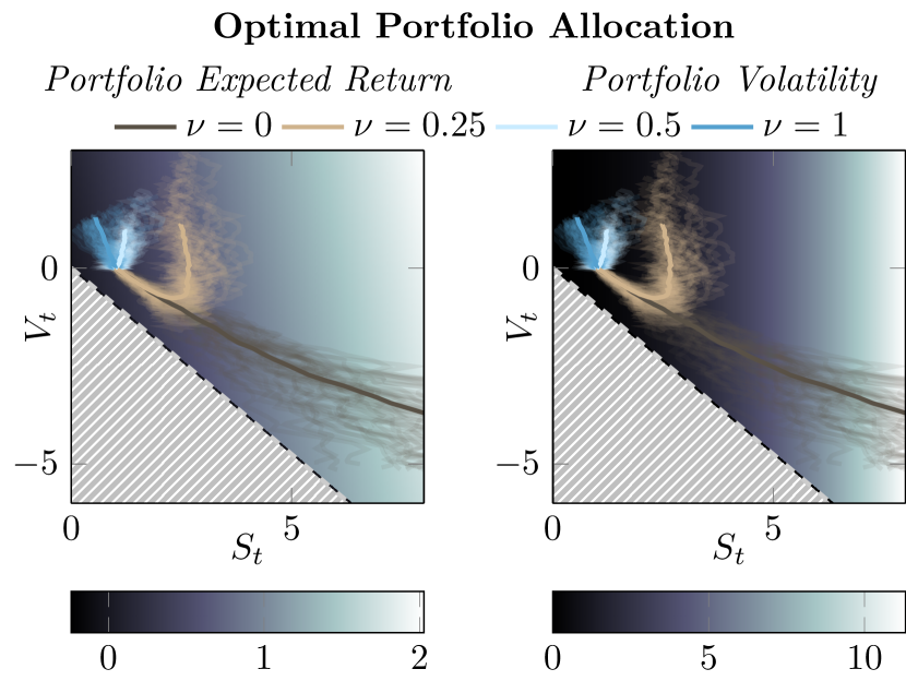
Figure 1: Realization of $(S_{t},V_{t})$ trajectories under learned strategies for four investors with different degrees of risk aversion, encoded in $\nu$, with a portfolio initialized at $(1,0)$ at time $0$. Different path realizations generated by the strategies are shown, along with their mean. [Left] Portfolio evolution against $r_{t}V_{t}+\mu_{t}S_{t}$ [Right] Portfolio evolution against $S_{t}^{2}\sigma$. Each strategy suits the corresponding risk aversion level.

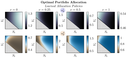
Figure 2: Learned buy–sell strategies $u_{\theta}^{i},u_{\theta}^{d}$ over the state–space $(S_{t},V_{t})$. The strategies are highly non–linear, and empirically agree with investment strategies at different risk aversion degrees. In example, the risk–seeking investor $\nu=0$ balances $u_{\theta}^{i},u_{\theta}^{d}$ to purchase the maximum amount of stock possible while remaining above the solvency line $V_{t}+(1-\alpha)S_{t}\geq 0$.

VI Related Work

Computing path–wise sensitivities through stochastic differential equations has been extensively explored in the literature. In particular, forward sensitivities with respect to initial conditions of solutions analogous to Proposition 1 were first introduced in [27] and extended for Itô case to parameters sensitivities in [39]. These approaches rely on integrating forward matrix–valued SDEs whose drift and diffusion require full Jacobians of $f_{\theta}$ and $g_{\theta}$ at each integration step. Thus, such methods poorly scales in computational cost with large number of parameters and high–dimensional–state regimes. This issue is averted by using backward adjoint sensitivity [40] where a vector–valued SDE is integrated backward and only requires vector–Jacobian products to be evaluated. In this direction, [28] proposed to solve the system’s backward SDE alongside the adjoint SDE to recover the value of the state $x_{t}$ and thus improve the algorithm memory footprint. Further, the approach is derived as a special case of [24, Theorem 2.4.1] and only considers criteria $J_{\theta}$ depending on the final state $x_{T}$ of the system.

Our stochastic adjoint process extends the results of [28] to integral criteria potentially exhibiting explicit parameter dependence. Further, we proposed a novel proving strategy based on classic variational analysis.

References

• [1] D. P. Bertsekas and S. Shreve, Stochastic optimal control: the discrete-time case, 2004.
• [2] H. Yu and D. P. Bertsekas, “Q-learning and policy iteration algorithms for stochastic shortest path problems,” Annals of Operations Research, vol. 208, no. 1, pp. 95–132, 2013.
• [3] Y. Wu and T. Shen, “Policy iteration algorithm for optimal control of stochastic logical dynamical systems,” IEEE transactions on neural networks and learning systems, vol. 29, no. 5, pp. 2031–2036, 2017.
• [4] S. Levine, “Reinforcement learning and control as probabilistic inference: Tutorial and review,” arXiv preprint arXiv:1805.00909, 2018.
• [5] E. Tse and M. Athans, “Adaptive stochastic control for a class of linear systems,” IEEE Transactions on Automatic Control, vol. 17, no. 1, pp. 38–52, 1972.
• [6] S. Peng and Z. Wu, “Fully coupled forward-backward stochastic differential equations and applications to optimal control,” SIAM Journal on Control and Optimization, vol. 37, no. 3, pp. 825–843, 1999.
• [7] M. A. Pereira and Z. Wang, “Learning deep stochastic optimal control policies using forward-backward sdes,” in Robotics: science and systems, 2019.
• [8] Z. Wang, K. Lee, M. A. Pereira, I. Exarchos, and E. A. Theodorou, “Deep forward-backward sdes for min-max control,” in 2019 IEEE 58th Conference on Decision and Control (CDC).   IEEE, 2019, pp. 6807–6814.
• [9] E. Weinan, “A proposal on machine learning via dynamical systems,” Communications in Mathematics and Statistics, vol. 5, no. 1, pp. 1–11, 2017.
• [10] R. T. Chen, Y. Rubanova, J. Bettencourt, and D. Duvenaud, “Neural ordinary differential equations,” arXiv preprint arXiv:1806.07366, 2018.
• [11] S. Massaroli, M. Poli, J. Park, A. Yamashita, and H. Asama, “Dissecting neural odes,” arXiv preprint arXiv:2002.08071, 2020.
• [12] S. Massaroli, M. Poli, M. Bin, J. Park, A. Yamashita, and H. Asama, “Stable neural flows,” arXiv preprint arXiv:2003.08063, 2020.
• [13] S. Peluchetti and S. Favaro, “Infinitely deep neural networks as diffusion processes,” in International Conference on Artificial Intelligence and Statistics.   PMLR, 2020, pp. 1126–1136.
• [14] L. Arnold, “Stochastic differential equations,” New York, 1974.
• [15] H. J. K. Kushner, H. J. Kushner, P. G. Dupuis, and P. Dupuis, Numerical methods for stochastic control problems in continuous time.   Springer Science & Business Media, 2001, vol. 24.
• [16] J. Schmidhuber, “Deep learning in neural networks: An overview,” Neural networks, vol. 61, pp. 85–117, 2015.
• [17] I. Goodfellow, Y. Bengio, A. Courville, and Y. Bengio, Deep learning.   MIT press Cambridge, 2016, vol. 1, no. 2.
• [18] L. Furieri, Y. Zheng, and M. Kamgarpour, “Learning the globally optimal distributed lq regulator,” in Learning for Dynamics and Control.   PMLR, 2020, pp. 287–297.
• [19] J. Bu, A. Mesbahi, M. Fazel, and M. Mesbahi, “Lqr through the lens of first order methods: Discrete-time case,” arXiv preprint arXiv:1907.08921, 2019.
• [20] N. G. Van Kampen, “Itô versus stratonovich,” Journal of Statistical Physics, vol. 24, no. 1, pp. 175–187, 1981.
• [21] B. Øksendal, “Stochastic differential equations,” in Stochastic differential equations.   Springer, 2003, pp. 65–84.
• [22] K. Itô, “Differential equations determining a markoff process,” J. Pan-Japan Math. Coll., vol. 1077, pp. 1352–1400, 1942.
• [23] R. Stratonovich, “A new representation for stochastic integrals and equations,” SIAM Journal on Control, vol. 4, no. 2, pp. 362–371, 1966.
• [24] H. Kunita, Stochastic Flows and Jump-Diffusions.   Springer.
• [25] E. Wong and M. Zakai, “On the convergence of ordinary integrals to stochastic integrals,” The Annals of Mathematical Statistics, vol. 36, no. 5, pp. 1560–1564, 1965.
• [26] R. C. Merton, “Lifetime portfolio selection under uncertainty: The continuous-time case,” The review of Economics and Statistics, pp. 247–257, 1969.
• [27] H. Kunita, Stochastic flows and stochastic differential equations.   Cambridge university press, 1997, vol. 24.
• [28] X. Li, T.-K. L. Wong, R. T. Chen, and D. Duvenaud, “Scalable gradients for stochastic differential equations,” arXiv preprint arXiv:2001.01328, 2020.
• [29] H. Robbins and S. Monro, “A stochastic approximation method,” The annals of mathematical statistics, pp. 400–407, 1951.
• [30] S. Ruder, “An overview of gradient descent optimization algorithms,” arXiv preprint arXiv:1609.04747, 2016.
• [31] C. De Sa, C. Re, and K. Olukotun, “Global convergence of stochastic gradient descent for some non-convex matrix problems,” in International Conference on Machine Learning.   PMLR, 2015, pp. 2332–2341.
• [32] Z. Allen-Zhu and E. Hazan, “Variance reduction for faster non-convex optimization,” in International conference on machine learning.   PMLR, 2016, pp. 699–707.
• [33] G. Smyrlis and V. Zisis, “Local convergence of the steepest descent method in hilbert spaces,” Journal of mathematical analysis and applications, vol. 300, no. 2, pp. 436–453, 2004.
• [34] H. K. Khalil, Nonlinear systems, vol. 3.
• [35] H. Liu and M. Loewenstein, “Optimal portfolio selection with transaction costs and finite horizons,” The Review of Financial Studies, vol. 15, no. 3, pp. 805–835, 2002.
• [36] D. P. Kingma and J. Ba, “Adam: A method for stochastic optimization,” arXiv preprint arXiv:1412.6980, 2014.
• [37] G. Mil’shtejn, “Approximate integration of stochastic differential equations,” Theory of Probability & Its Applications, vol. 19, no. 3, pp. 557–562, 1975.
• [38] J. Nocedal and S. Wright, Numerical optimization.   Springer Science & Business Media, 2006.
• [39] E. Gobet and R. Munos, “Sensitivity analysis using itô–malliavin calculus and martingales, and application to stochastic optimal control,” SIAM Journal on control and optimization, vol. 43, no. 5, pp. 1676–1713, 2005.
• [40] M. Giles and P. Glasserman, “Smoking adjoints: fast evaluation of greeks in monte carlo calculations,” 2005.