Complex Ground-State and Excitation Energies in Coupled-Cluster Theory

Abstract

Since in coupled-cluster (CC) theory ground-state and excitation energies are eigenvalues of a non-Hermitian matrix, these energies can in principle take on complex values. In this paper we discuss the appearance of complex energy values in CC calculations from a mathematical perspective. We analyze the behaviour of the eigenvalues of Hermitian matrices that are perturbed (in a non-Hermitian manner) by a real parameter. Based on these results we show that for CC calculations with real-valued Hamiltonian matrices the ground-state energy generally takes a real value. Furthermore, we show that in the case of real-valued Hamiltonian matrices complex excitation energies only occur in the context of conical intersections. In such a case, unphysical consequences are encountered such as a wrong dimension of the intersection seam, large numerical deviations from full configuration-interaction (FCI) results, and the square-root-like behaviour of the potential surfaces near the conical intersection. In the case of CC calculations with complex-valued Hamiltonian matrix elements, it turns out that complex energy values are to be expected for ground and excited states when no symmetry is present. We confirm the occurrence of complex energies by sample calculations using a six-state model and by CC calculations for the $\mathrm{H_{2}O}$ molecule in a strong magnetic field. We furthermore show that symmetry can prevent the occurrence of complex energy values. Lastly, we demonstrate that in most cases the real part of the complex energy values provides a very good approximation to the FCI energy.

I Introduction

Coupled-cluster (CC) theoryShavitt and Bartlett (2009) is one of the most widely used quantum-chemical methods for high-accuracy computations of energies and properties. As a post-Hartree-Fock method, CC theory focuses on an adequate, i.e., size-extensive, treatment of electron correlation and ensures this by applying the exponential of an excitation operator, i.e., the so-called cluster operator, to a reference determinant, most often chosen as the Hartree-Fock (HF) wave function. The equation-of-motion CC (EOM-CC) ansatzEmrich (1981); Stanton and Bartlett (1993a); Comeau and Bartlett (1993); Rico and Head-Gordon (1993); Shavitt and Bartlett (2009) extends ground-state CC theory to excited states. The key step lies in the similarity transformation of the electronic Hamiltonian with the exponential of the cluster operator followed by a diagonalization of the resulting effective Hamiltonian. However, as this transformation is not unitary, Hermiticity is lost and as a consequence complex excitation energies can in principle be obtained in an EOM-CC calculation.

HättigHättig (2005) was the first to note that the lack of Hermiticity can lead in EOM-CC calculations to a qualitatively wrong description of potential energy surfaces in the vicinity of conical intersections. Using a two-state model, Hättig predicted that the energies of the two involved states pass through a point of degeneracy and then enter an area where their values are complex. Köhn and TajtiKöhn and Tajti (2007) confirmed this scenario based on EOM-CC calculations for two excited states of formaldehyde ($\mathrm{CH_{2}O}$). In addition, they observed a square-root like behaviour of the EOM-CC energies of the two states near the intersection and showed that the eigenvectors associated with the two degenerate states become linearly dependent. Kjønstadt et al.Kjønstad et al. (2017) later demonstrated that the EOM-CC description of a conical intersection is not necessarily always flawed but depends on whether the similarity-transformed Hamiltonian matrix is defective or not at the point of degeneracy. A qualitatively correct description is only observed in the case of a non-defective matrix. We also note that complex energies have so far not been observed in ground-state CC calculations.

In this paper we explain why complex energies have not been observed in CC calculations except close to conical intersections and discuss in which cases they can be expected. We analyze the behavior of the eigenvalues of general real and complex matrices and apply the corresponding mathematical tools to CC theory. Apart from results that are already discussed in the literature, this approach also leads to additional knowledge about the shape of the potential surfaces near conical intersections and about the occurrence of complex eigenvalues in the case of Hamiltonian matrices with complex-valued entries. The latter allows us to draw conclusions about the occurrence of complex energy values in the case of CC calculations for systems in a finite magnetic fieldStopkowicz et al. (2015); Hampe and Stopkowicz (2017); Hampe et al. (2020) and for relativistic CC calculations that include spin-orbit coupling.Visscher et al. (1996); Wang et al. (2008); Shee et al. (2018); Liu et al. (2018a)
The present work begins with a discussion of a several mathematical definitions and theorems needed for our investigation, like the perturbative analysis of the eigenvalues of a matrix. In section II, the basics of CC theory and EOM-CC theory are briefly reviewed. Section III analyzes the occurrence of eigenvalues in the case of a real-valued Hamiltonian matrix. It is shown that complex energy values can only occur in the context of conical intersections. Using the mathematical tools presented in section II, consequences of the occurrence of complex values such as a wrong dimension of the intersection seam and a wrong shape of the potential energy surfaces around the conical intersection are derived and analyzed. Section IV examines the occurrence of complex energy values in the case that the Hamiltonian matrix has complex-valued entries, as it happens in the case of finite magnetic-field and relativistic CC calculations. Here, we perform and discuss example calculations that show that the appearance of complex energy values is common.We also show that the real part of a complex energy value nevertheless provides a useful approximation to the actual energy. Finally, we demonstrate that symmetry typically ensures that the resulting CC energy values are real.

II Theory

Subsection II.1 reviews the required mathematical background of eigenvalue theory and subsection II.2 outlines CC theory.

II.1 Mathematical background

In the following part two basic series expansions, the well-known Taylor series and the lesser known Puiseux series, are discussed.Wilkinson (1965); Kato (1995); Wall (2004); Thomas (2018)

Definition II.1.

A formal series expansion

$$y(x)=y_{0}+a_{1}x+a_{2}x^{2}+a_{3}x^{3}+\cdots,$$

where $a_{i}\in\mathbb{C},\hskip 5.69046ptx\in\mathbb{R},$ is denoted as a Taylor series at point $x=0$.
A formal series expansion of the form

$$y(x)=y_{0}+a_{1}(x^{\frac{1}{m}})_{k}+a_{2}(x^{\frac{1}{m}})_{k}^{2}+\cdots,$$

where $m\in\mathbb{N}$, $m>1$, $a_{i}\in\mathbb{C}$ and $x\in\mathbb{R}$, is called a Puiseux series at point $x=0$.
Here $(x^{\frac{1}{m}})_{k}:=|x|^{\frac{1}{m}}e^{i\frac{2\pi k+\pi}{m}}$ is an $m$-th root of $x$.

It is obvious that different choices for the root $(x^{\frac{1}{m}})_{k}$ lead to different branches of the series. All branches are continuous and analytic in all points except for $x=0$.
We call a matrix analytically dependent on the parameter $\epsilon$ if all matrix entries can be described by a Taylor series depending on $\epsilon$. A change of the matrix entries due to a variation of $\epsilon$ is called an analytic matrix perturbation. The following theoremKato (1995); Thomas (2018) states that the change of the eigenvalues caused by an analytic matrix perturbation can be described either by a Taylor series or by a Puiseux series.

Theorem II.2.

Let $A(\epsilon)\in\mathbb{C}(n\times n)$ be a matrix whose entries depend analytically on one real parameter $\epsilon$. Furthermore, let $\lambda_{i}(\epsilon)$ be an eigenvalue of $A(\epsilon)$. Then the following holds:

• Let $\lambda_{i}(0)$ be a single eigenvalue. Then there exists a neighbourhood $U$ of $(0,\lambda_{i}(0))$, where exactly one single eigenvalue exists for every $\epsilon\in U$. The dependence of the eigenvalue on $\epsilon$ can be expressed by means of a Taylor series as

  $$\lambda_{i}(\epsilon)=\lambda(0)+p_{i1}\epsilon+p_{i2}\epsilon^{2}+p_{i3}\epsilon^{3}+\cdots.$$ (1)

• Let $\lambda(0)=\lambda_{1}(0)=\lambda_{2}(0)=...=\lambda_{m}(0)$ be a multiple eigenvalue. Then there exists a neighbourhood $U$ of $(0,\lambda(0))$, such that for each fixed $\epsilon$ there exist exactly $m$ eigenvalues of $A(\epsilon)$ in $U$. The dependence of each eigenvalue on $\epsilon$ can be described either by a Taylor series (as in Eq. (1)) or by one of the branches, $\lambda_{i}(\epsilon)$, of a Puiseux series $\lambda(\epsilon)$, which has the form

  $$\lambda(\epsilon)=\lambda(0)+p_{i1}\epsilon^{\frac{1}{\widetilde{m}}}+p_{i2}\epsilon^{\frac{2}{\widetilde{m}}}+\cdots$$ (2)

  with $\widetilde{m}\leq m$. In the case that one of the branches of a Puiseux series is a solution of the eigenvalue problem $A(\epsilon)v(\epsilon)=\lambda(\epsilon)v(\epsilon)$, the other possible branches $\lambda_{i}(\epsilon)$ fulfill the eigenvalue equation, too.

We illustrate the stated theorem by analyzing the behaviour of the eigenvalues of the following $2\times 2$ matrix

$$A_{1}(\epsilon)=\begin{pmatrix}1-\epsilon&1-\epsilon\\ 1.5\epsilon&1+\epsilon\end{pmatrix}$$

which analytically depends on a real parameter $\epsilon$. For $\epsilon\neq 0$ the matrix $A(\epsilon)$ has single eigenvalues. They develop in analytic manner as a function of the perturbation parameter (see theorem II.2 and Figure 1). For $\epsilon=0$ a multiple eigenvalue occurs. The series expansion at this point is

$$\lambda(\epsilon)\approx 1+1.225\epsilon^{\frac{1}{2}}-0.204{\epsilon}^{\frac{3}{2}}-0.017{\epsilon}^{\frac{5}{2}}-\cdots.$$ (3)

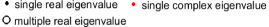
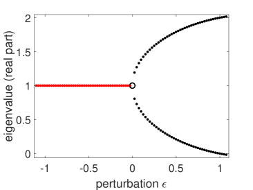
Figure 1: Real and imaginary part of the eigenvalues of $A_{1}(\epsilon)$.

According to this series expansion the eigenvalues develop in a continuous manner. From the same series expansion as well as from Figure 1 we also see that the square-root term dominates the behaviour of the eigenvalues near the branching point $\epsilon=0$. In case of such a shape we speak of square-root like behaviour in the broader context. Consequences of the square-root like behaviour are that the function $\lambda(\epsilon)$ is not differentiable at the point $\epsilon=0$ and that a small change in $\epsilon$ leads to a large change in the eigenvalues.
In the given example, the eigenvectors of the matrix $A_{1}(0)$ are linearly dependent. Such a matrix is called defective, whereas a matrix is called non-defective if its eigenvectors span a complete base of the vector space (i.e., the matrix is diagonalizable).Golub and Loan (2013) In case that the matrix is non-defective at the point where multiple eigenvalues occur a square-root like behaviour of the eigenvalues cannot appear. This is ensured by the following theorem by Kato:Kato (1995)

Theorem II.3 (Kato).

Let $A(\epsilon)\in\mathbb{C}(n\times n)$ be a non-defective matrix depending analytically on $\epsilon$. Let $\lambda(0)=\lambda_{1}(0)=\lambda_{2}(0)=...=\lambda_{m}(0)$ be a multiple eigenvalue. Then, each eigenvalue $\lambda_{i}(\epsilon)$ in the neighbourhood of $(0,\lambda(0))$ can be represented in one of the following two ways:

• by a Taylor series

  $$\lambda_{i}(\epsilon)=\lambda(0)+p_{i1}\epsilon+p_{i2}\epsilon^{2}+p_{i3}\epsilon^{3}+\cdots.$$

• or by a branch of a Puiseux series, where the linear term dominates the series expansion:

  $$\lambda(\epsilon)=\lambda(0)+p_{i1}\epsilon+p_{i2}\epsilon^{1+\frac{1}{\widetilde{m}}}+p_{i3}\epsilon^{1+\frac{2}{\widetilde{m}}}+\cdots$$

with $\widetilde{m}\leq m$. In both cases $\lambda_{i}(\epsilon)$ is differentiable at the point $\epsilon=0$. Note that the second case equals the first case if $\widetilde{m}=1$.

Thus, the question whether or not a matrix is defective plays a decisive role in the appearance of the function $\lambda(\epsilon)$.

In the previous example, the transition from complex to real eigenvalues, caused by the variation of $\epsilon$, proceeds via a multiple eigenvalue. This statement is generally valid and is explained in detail by means of the following theorem.

Theorem II.4.

Let $\lambda_{i}(\epsilon)$ be an eigenvalue of $A(\epsilon)\in\mathbb{C}(n\times n)$. Furthermore, there exist $a,b>0$ such that $\lambda_{i}(\epsilon)$ takes a real value for all $\epsilon\in[-a,0]$ and $\lambda_{i}(\epsilon)$ takes a complex value for all $\epsilon\in(0,b]$. Then:

1. In a neighbourhood of $\epsilon=0$ the eigenvalue $\lambda_{i}(\epsilon)$ can be represented by a branch of a Puiseux series.

2. For $\epsilon=0$ a multiple eigenvalue occurs.

A proof can be found in the Appendix A.

In the case that the matrix $A(\epsilon)$ has only real entries, further properties can be specified for the behaviour of an eigenvalue $\lambda(\epsilon)$:

Theorem II.5.

Let $A(\epsilon)$ be a matrix with only real entries for all $\epsilon\in(-r,r)$, then:

• Let $\lambda(\epsilon)$ be a complex eigenvalue of $A(\epsilon)$, then the complex-conjugated eigenvalue ${\lambda^{*}(\epsilon)}$ is also an eigenvalue of $A(\epsilon)$.

• Let $\lambda_{i}(0)$ be a single real eigenvalue of $A(0)$, then a neighbourhood $U$ of $(0,\lambda(0))$ exists, such that $\lambda_{i}(\epsilon)$ takes only real values in $U$.

The proof can also be found in the Appendix A.

II.2 Coupled-cluster theory

The electronic states $\ket{\Psi_{k}}$ of a molecule together with their associated energy values $E_{k}$ are determined by the electronic Schrödinger equation:

$$\hat{H}\ket{\Psi_{k}}=E_{k}\ket{\Psi_{k}},\hskip 14.22636ptk\geq 0.$$

In second quantization, the Hamiltonian $\hat{H}$ takes the formShavitt and Bartlett (2009)

$$\hat{H}=\sum_{p,q}h_{pq}\hat{a}_{p}^{\dagger}\hat{a}_{p}+\frac{1}{4}\sum_{p,q,r,s}g_{pqrs}\hat{a}_{p}^{\dagger}\hat{a}_{q}^{\dagger}\hat{a}_{s}\hat{a}_{r}$$ (4)

with $\{p,q,\cdots\}$ representing the index set of the underlying molecular spin orbitals $\{\varphi_{p},\varphi_{q},...\}$ and $\hat{a}^{\dagger}_{p}$ and $\hat{a}_{p}$ as the corresponding elementary creation and annihilation operators. In Eq. (4), $h_{pq}$ and $g_{pqrs}$ denote the matrix elements of the one ($\hat{h}$) and two-electron ($\hat{g}$) operator which constitute the Hamiltonian in first quantization. They are calculated using the underlying set of one-electron functions $\{\varphi_{p},\varphi_{q},...\}$ and the operators $\hat{h}$ and $\hat{g}$ via

$$h_{pq} =\bra{\varphi_{p}}\hat{h}\ket{\varphi_{q}}$$ (5)

$$g_{pqrs} =\bra{\varphi_{p}\varphi_{q}}\hat{g}\ket{\varphi_{r}\varphi_{s}}-\bra{\varphi_{p}\varphi_{q}}\hat{g}\ket{\varphi_{s}\varphi_{r}}.$$ (6)

The exact definitions of the one- and two-electron operators $\hat{h}$ and $\hat{g}$ depend on the context. They are different for traditional nonrelativistic CC calculations and those that incorporate relativistic effects,Dyall and Fægri Jr. (2007) and for cases in which a finite magnetic field is present.Stopkowicz et al. (2015); Hampe and Stopkowicz (2017, 2019); Hampe et al. (2020) For our discussion the general representation given in Eq. (4) is sufficient. However, it must be noted that the choice of the operators $\hat{h}$ and $\hat{g}$ plays a decisive role as to whether the matrix elements $h_{pq}$ and $g_{pqrs}$ are real- or complex-valued.

In CC theory,Bartlett and Musiał (2007); Shavitt and Bartlett (2009); Schneider (2009) the ground-state wave function is obtained by applying the exponential of the cluster operator ${\hat{T}}$ to a reference Slater determinant $\psi_{0}$:

$$\ket{\Psi_{\mathrm{CC}}}=e^{\hat{T}}\ket{\psi_{0}}.$$ (7)

In second quantization, the cluster operator $\hat{T}$ is given as

$$\hat{T} =\hat{T}_{1}+\hat{T}_{2}+\cdots+\hat{T}_{n}$$ (8)

$$=\sum_{n=1}^{N}\Big{(}\frac{1}{n!}\Big{)}^{2}\sum_{i,j,...}\ \sum_{a,b,...}t_{ij...}^{ab...}\hat{a}_{a}^{\dagger}\hat{a}_{i}\hat{a}_{b}^{\dagger}\hat{a}_{j}\cdots.$$ (9)

with the number of electrons $N$ and $i,j,k,\dots$ as well as $a,b,c,\dots$ referring to the occupied and virtual space, respectively. The amplitudes $t_{ij...}^{ab...}$ of the cluster operator are obtained by solving the CC equations

$$\bra{\psi_{I}}e^{\hat{T}}\hat{H}e^{-\hat{T}}\ket{\psi_{0}}=0$$ (10)

for all Slater determinants $\psi_{I}$ of the FCI space. Under certain conditions, which are in particular that the Slater determinants $\psi_{I}$ as well as the matrix elements $h_{pq}$ and $g_{pqrs}$ are real-valued, this non-linear system of equations has a locally unique real solution for the amplitudes $t_{ij...}^{ab...}$. Schneider (2009) In this case the CC ground-state energy $E_{\mathrm{CC}}=\bra{\psi_{0}}e^{-\hat{T}}\hat{H}e^{\hat{T}}\ket{\psi_{0}}$ is also real.

For computational reasons the cluster operator is usually truncated after a few terms and the CC equations (Eq. (10)) are solved only for the excitations included in $\hat{T}$. For example, by choosing $\hat{T}=\hat{T}_{1}+\hat{T}_{2}$ and by solving the CC equations for single and double excitations, the well-known CC singles and doubles (CCSD) methodPurvis III and Bartlett (1982) results. The statement that the system of equations (Eq. (10)) has a locally unique real solution, (if the same conditions hold as before) is also correct for a truncated operator $\hat{T}$.

Based on CC theory, the EOM-CC approachRowe (1968); Emrich (1981); Stanton and Bartlett (1993b); Comeau and Bartlett (1993); Rico and Head-Gordon (1993) is a popular choice for the calculation of excitation energies with the following ansatz for the corresponding $k$-th excited-state wave function:

$$\ket{\Psi_{\mathrm{exc}}^{(k)}}=\hat{R}^{(k)}\ket{\Psi_{\mathrm{CC}}}=\hat{R}^{(k)}e^{\hat{T}}\ket{\psi_{0}}.$$ (11)

The cluster operator $\hat{T}$ is taken from a preceding CC ground-state calculation and $\hat{R}^{(k)}$ is a linear excitation operator that differs from $\hat{T}$ only by the constant contribution $\hat{R}_{0}^{(k)}$:

$$\hat{R}^{(k)}=\hat{R}^{(k)}_{0}+\hat{R}^{(k)}_{1}+\hat{R}^{(k)}_{2}+\cdots.$$ (12)

Both the amplitudes of the excitation operator $\hat{R}^{(k)}$, as the entries in the eigenvector $\vec{r}^{(k)}$, and the excited-state energies $E_{k}$ are obtained by solving the eigenvalue problem

$$\bar{H}_{\mathrm{FCI}}\vec{r}^{(k)}=E_{k}\vec{r}^{(k)},$$ (13)

where $\bar{H}_{\mathrm{FCI}}$ is the matrix representation of the similarity-transformed Hamilton operator $\hat{\bar{H}}=e^{\hat{T}}\hat{H}e^{-\hat{T}}$ in the FCI space.

To render EOM-CC calculations feasible the excitation operator $\hat{R}^{(k)}$ is usually truncated at the same level as $\hat{T}$. The amplitudes of $\hat{R}^{(k)}$ and the energy values are then determined by the eigenvectors and eigenvalues of the truncated matrix

$$\bar{H}_{\mathrm{P}}=P\bar{H}_{\mathrm{FCI}}P^{\dagger}=\begin{pmatrix}E_{\mathrm{CC}}&\hskip 8.5359pt&*\\ 0\\ \mathchoice{\vbox{\kern 3.69444pt\vbox to8.83328pt{\offinterlineskip\hbox{\set@color$\displaystyle.$}\vfill\hbox{\set@color$\displaystyle.$}\vfill\hbox{\set@color$\displaystyle.$}}}}{\vbox{\kern 3.69444pt\vbox to8.83328pt{\offinterlineskip\hbox{\set@color$\textstyle.$}\vfill\hbox{\set@color$\textstyle.$}\vfill\hbox{\set@color$\textstyle.$}}}}{\vbox{\kern 2.91943pt\vbox to6.84993pt{\offinterlineskip\hbox{\set@color$\scriptstyle.$}\vfill\hbox{\set@color$\scriptstyle.$}\vfill\hbox{\set@color$\scriptstyle.$}}}}{\vbox{\kern 2.40276pt\vbox to5.52771pt{\offinterlineskip\hbox{\set@color$\scriptscriptstyle.$}\vfill\hbox{\set@color$\scriptscriptstyle.$}\vfill\hbox{\set@color$\scriptscriptstyle.$}}}}&&**\\ 0\end{pmatrix},$$ (14)

where the matrix $P=\left(\begin{smallmatrix}1&\cdots&0&\cdots&0\\ \mathchoice{\vbox{\kern 2.58612pt\vbox to6.1833pt{\offinterlineskip\hbox{\set@color$\displaystyle.$}\vfill\hbox{\set@color$\displaystyle.$}\vfill\hbox{\set@color$\displaystyle.$}}}}{\vbox{\kern 2.58612pt\vbox to6.1833pt{\offinterlineskip\hbox{\set@color$\textstyle.$}\vfill\hbox{\set@color$\textstyle.$}\vfill\hbox{\set@color$\textstyle.$}}}}{\vbox{\kern 2.04362pt\vbox to4.79498pt{\offinterlineskip\hbox{\set@color$\scriptstyle.$}\vfill\hbox{\set@color$\scriptstyle.$}\vfill\hbox{\set@color$\scriptstyle.$}}}}{\vbox{\kern 1.68195pt\vbox to3.8694pt{\offinterlineskip\hbox{\set@color$\scriptscriptstyle.$}\vfill\hbox{\set@color$\scriptscriptstyle.$}\vfill\hbox{\set@color$\scriptscriptstyle.$}}}}&\mathinner{\mathchoice{\vbox{\kern 2.58612pt\vbox to6.1833pt{\offinterlineskip\hbox{$\displaystyle\mathpunct{.}$}\vfill\hbox{$\displaystyle\mathpunct{\kern 1.94444pt}\mathpunct{.}$}\vfill\hbox{$\displaystyle\mathpunct{\kern 1.94444pt}\mathpunct{\kern 1.94444pt}\mathpunct{.}$}}}}{\vbox{\kern 2.58612pt\vbox to6.1833pt{\offinterlineskip\hbox{$\textstyle\mathpunct{.}$}\vfill\hbox{$\textstyle\mathpunct{\kern 1.94444pt}\mathpunct{.}$}\vfill\hbox{$\textstyle\mathpunct{\kern 1.94444pt}\mathpunct{\kern 1.94444pt}\mathpunct{.}$}}}}{\vbox{\kern 2.04362pt\vbox to4.79498pt{\offinterlineskip\hbox{$\scriptstyle\mathpunct{.}$}\vfill\hbox{$\scriptstyle\mathpunct{\kern 1.36111pt}\mathpunct{.}$}\vfill\hbox{$\scriptstyle\mathpunct{\kern 1.36111pt}\mathpunct{\kern 1.36111pt}\mathpunct{.}$}}}}{\vbox{\kern 1.68195pt\vbox to3.8694pt{\offinterlineskip\hbox{$\scriptscriptstyle\mathpunct{.}$}\vfill\hbox{$\scriptscriptstyle\mathpunct{\kern 0.97221pt}\mathpunct{.}$}\vfill\hbox{$\scriptscriptstyle\mathpunct{\kern 0.97221pt}\mathpunct{\kern 0.97221pt}\mathpunct{.}$}}}}\mkern 3.0mu}&\mathchoice{\vbox{\kern 2.58612pt\vbox to6.1833pt{\offinterlineskip\hbox{\set@color$\displaystyle.$}\vfill\hbox{\set@color$\displaystyle.$}\vfill\hbox{\set@color$\displaystyle.$}}}}{\vbox{\kern 2.58612pt\vbox to6.1833pt{\offinterlineskip\hbox{\set@color$\textstyle.$}\vfill\hbox{\set@color$\textstyle.$}\vfill\hbox{\set@color$\textstyle.$}}}}{\vbox{\kern 2.04362pt\vbox to4.79498pt{\offinterlineskip\hbox{\set@color$\scriptstyle.$}\vfill\hbox{\set@color$\scriptstyle.$}\vfill\hbox{\set@color$\scriptstyle.$}}}}{\vbox{\kern 1.68195pt\vbox to3.8694pt{\offinterlineskip\hbox{\set@color$\scriptscriptstyle.$}\vfill\hbox{\set@color$\scriptscriptstyle.$}\vfill\hbox{\set@color$\scriptscriptstyle.$}}}}&&\mathchoice{\vbox{\kern 2.58612pt\vbox to6.1833pt{\offinterlineskip\hbox{\set@color$\displaystyle.$}\vfill\hbox{\set@color$\displaystyle.$}\vfill\hbox{\set@color$\displaystyle.$}}}}{\vbox{\kern 2.58612pt\vbox to6.1833pt{\offinterlineskip\hbox{\set@color$\textstyle.$}\vfill\hbox{\set@color$\textstyle.$}\vfill\hbox{\set@color$\textstyle.$}}}}{\vbox{\kern 2.04362pt\vbox to4.79498pt{\offinterlineskip\hbox{\set@color$\scriptstyle.$}\vfill\hbox{\set@color$\scriptstyle.$}\vfill\hbox{\set@color$\scriptstyle.$}}}}{\vbox{\kern 1.68195pt\vbox to3.8694pt{\offinterlineskip\hbox{\set@color$\scriptscriptstyle.$}\vfill\hbox{\set@color$\scriptscriptstyle.$}\vfill\hbox{\set@color$\scriptscriptstyle.$}}}}\\ 0&\cdots&1&\cdots&0\\ \end{smallmatrix}\right)$ projects $\bar{H}_{\mathrm{FCI}}$ onto the space of Slater determinants considered by $\hat{R}^{(k)}$.

Since the first column, apart from the first entry, vanishes due to the CC equations, the CC ground-state energy $E_{\mathrm{CC}}$ equals the lowest eigenvalue $E_{0}$ of the matrix $\bar{H}_{\mathrm{P}}$. Thus, the analysis of both the CC ground-state energy $E_{\mathrm{CC}}$ as well as the EOM-CC excitation energies $E_{k}$ can be performed by means of an analysis of the eigenvalues of $\bar{H}_{\mathrm{P}}$.
A frequently used EOM-CC scheme is to choose $\hat{T}=\hat{T}_{1}+\hat{T}_{2}$ and $\hat{R}=\hat{R}_{0}+\hat{R}_{1}+\hat{R}_{2}$ which leads to the EOM-CCSD model.Stanton and Bartlett (1993b); Comeau and Bartlett (1993); Rico and Head-Gordon (1993) In the present context this model will be used as a representative for all EOM-CC methods. In contrast to Hermitian quantum-chemical methods (e.g., FCI or truncated configuration interaction (CI)), it cannot be ensured that the energy values of the EOM-CC method are real-valued,Hättig (2005); Köhn and Tajti (2007) as the matrix $\bar{H}_{\mathrm{P}}$ is usually not Hermitian.

III Complex energies in case of a real-valued $\bar{H}_{\mathrm{P}}$ matrix

According to the previous section, it depends on the matrix $\bar{H}_{\mathrm{P}}$ whether the EOM-CC energy values (including the CC ground-state energy) are real or not. For the sake of simplicity we limit our discussion to the EOM-CCSD model. Conceptually, analogous results can be obtained for other EOM-CC methods (e.g., EOM-CCSDT,Kowalski and Piecuch (2001); Kucharski et al. (2001); Bomble et al. (2004) EOM-CCSDTQ,Kállay and Gauss (2004) etc.) by means of a similar analyses. In this section it is assumed that the entries of the matrix $\bar{H}_{\mathrm{FCI}}$ are real. This applies, for example, if the matrix elements $h_{pq}$, $g_{pqrs}$ and the underlying one-electron wave functions $\{\varphi_{p},\varphi_{q},...\}$ are real-valued (see section II.2). As a first approach to analyze the appearance of complex energy values, we construct a continuous connection between the FCI and EOM-CCSD energy values.

III.1 Connection between FCI and EOM-CCSD energy values

Let $\bar{H}_{\mathrm{FCI}}$ be the matrix representation of the similarity transformed Hamiltonian in the FCI space and $\bar{H}_{\mathrm{P}}=P\bar{H}_{\mathrm{FCI}}P^{\dagger}$ the truncated $\bar{H}_{\mathrm{FCI}}$ matrix as described in section II.2. The eigenvalues of $\bar{H}_{\mathrm{FCI}}$, hereafter also referred to as FCI eigenvalues, are the energy eigenvalues of the FCI method. The eigenvalues of the matrix $\bar{H}_{\mathrm{P}}$, hereafter referred to as CCSD eigenvalues, are the energy values of the EOM-CCSD method. We now establish a continuous connection between the FCI and CCSD eigenvalues by switching on a perturbation $S$ using a real parameter $\varepsilon$. Formally, this can be described by

$$\bar{H}(\varepsilon):=\bar{H}_{\mathrm{FCI}}+\varepsilon\underbrace{\begin{pmatrix}0&*\\ **&***\\ \end{pmatrix}}_{S},$$

where the matrix $S$ is defined by

$$S:=\left(\begin{smallmatrix}\bar{H}_{\mathrm{P}}&0\\ 0&D\end{smallmatrix}\right)-\bar{H}_{\mathrm{FCI}}$$ (15)

The matrix block $D$ is chosen as a diagonal matrix with the otherwise irrelevant FCI eigenvalues on the diagonal in order to isolate them from the relevant eigenvalues. Hence for $\varepsilon=0$ the matrix $\bar{H}(\varepsilon)$ returns the FCI eigenvalues. The perturbation is invoked by $\varepsilon>0$. For $\varepsilon=1$ the matrix $\bar{H}(\varepsilon)$ provides the CCSD eigenvalues.
Based on the mathematical results from section II.1, the transition from the FCI to the CCSD eigenvalues can be characterized in more detail. The FCI eigenvalues are connected to the CCSD eigenvalues in a continuous manner (see theorem II.2). For the connection it applies that in the neighbourhood of each simple real eigenvalue only real eigenvalues occur (see theorem II.5) and that complex eigenvalues arise only if two eigenvalues coincide (see theorem II.4). Here it plays an important role for the development of the eigenvalues whether the matrix is defective at this point or not (see theorem II.3). Altogether the following five scenarios can be sketched:

Figure 2: Schematic representation of the possible connections between the FCI and CCSD energy values in the case where the matrix $\bar{H}(\epsilon)$ has only real entries.

• A simple FCI eigenvalue is sufficiently well separated from the other FCI eigenvalues so that it does not coincide with any other on the connection to the CCSD eigenvalues. Then the corresponding EOM-CCSD energy value is simple and real.

• Two eigenvalues on the connection between FCI and CCSD eigenvalues coincide without complex eigenvalues arising in the neighbourhood of the multiple eigenvalue. Even then the energy value of the EOM-CCSD method is real as in scenario a).

• On the connection between FCI and CCSD eigenvalues two eigenvalues coincide for an $\varepsilon_{0}\in[0,1]$ for which the matrix $\bar{H}(\varepsilon_{0})$ is defective and for which in the neighbourhood of $\varepsilon_{0}$ complex eigenvalues occur. In contrast to scenarios a) and b), the series development of the eigenvalue $\lambda(\varepsilon_{0})$ is then dominated by the term $\varepsilon^{0.5}$ (see theorem II.4). This leads to large differences between CCSD and FCI eigenvalues and to complex CCSD eigenvalues.

• Similar to scenario c) complex eigenvalues occur, but the matrix is not defective at the point where multiple eigenvalues occur. In this case, a complex part of the eigenvalue is generated at the earliest by the term $\varepsilon^{\frac{3}{2}}$ in the series development (see theorem II.3).

• The FCI method provides a multiple eigenvalue. Due to the fact that the $\bar{H}_{\mathrm{FCI}}$ matrix is non-defective (since it is a similarity transformation of the Hermitian matrix $H_{\mathrm{FCI}}$), the series development of $\lambda(0)$ is dominated by the term $\varepsilon^{1}$. Both complex or real CCSD energy values are possible.

The connection between FCI and CCSD eigenvalues can be illustrated as in Figure 2. A black line indicates here real eigenvalues for the matrix $H(\varepsilon)$, a red line the appearance of a pair of complex-conjugated eigenvalues, and „$\circ$ “ marks the occurrence of a multiple eigenvalue.
Two facts become clear from this analysis. First, if a FCI energy value is well separated from all others the corresponding EOM-CCSD energy value is real (see Scenario a)). This is the reason why complex energy values rarely occur in EOM-CCSD calculations. Together with the assumption that the energy gap between ground-state energy and the first excitation energy is sufficiently large it leads to the fact that the CC ground-state energy is real-valued. This is in agreement with the statement cited in Section II.2 from Schneider’s results.Schneider (2009) Second, if a complex EOM-CCSD energy value occurs, a square-root like behaviour results, as in scenario d), caused by the term $\varepsilon^{\frac{1}{2}}$ in the series expansion of the eigenvalue. This leads to large discrepancies between FCI and CCSD energy values.

In practice, the described connection between the FCI and CCSD methods is difficult to investigate. For this reason, we introduce in the following an artificial system, which consists of four electrons and six possible states. The FCI space is thus spanned by six Slater determinants $\{\psi_{0},...,\psi_{5}\}$. The situation can be illustrated with a MO-like representation:
$\psi_{0}$        $\psi_{1}$        $\psi_{2}$        $\psi_{3}$        $\psi_{4}$        $\psi_{5}$
By specifying the matrix representation $H_{\mathrm{FCI}}$ of the Hamiltonian, the system is fully described.

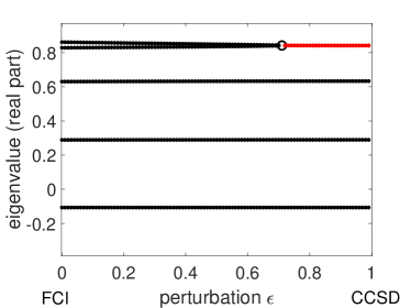
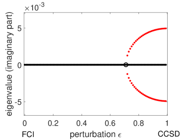
Figure 3: Connection between FCI and CCSD eigenvalues for an sample Hamiltonian, defined by the matrix representation $H_{1}$ (see Appendix B) for the 6-state model discussed in the text.

Using this model, we test the previously presented connection between the FCI and CCSD energy values by actual calculations. The FCI eigenvalues are obtained from the chosen $6\times 6$ matrix representation ${H}_{\mathrm{FCI}}$ of the Hamiltonian (see Appendix B for details of ${H}_{\mathrm{FCI}}$). The CCSD eigenvalues result from the truncated $5\times 5$ matrix $\bar{H}_{\mathrm{P}}$ (see Section II.2). The amplitudes of $\hat{T}_{2}$ are determined via a standard CC calculation. The results of the calculation are shown in Figure 3 and are consistent with the theoretical predictions. The lowest three energy values are well-separated from all others, no complex energy values occur and a deviation between FCI and CCSD energy values is hardly recognizable. However, the two highest energy values are not well separated in the FCI solution. Here a multiple eigenvalue occurs for $\bar{H}(\varepsilon\approx 0.7)$ and for the CCSD method complex energy values arise. As predicted, a square-root-like behaviour can be observed and the difference between the energy values of the FCI and CCSD solution is clearly visible.

III.2 Complex energy values in the vicinity of conical intersections

The occurrence of a multiple eigenvalue in CC calculations implies that two different states of the molecule have close-lying energy values and that the two corresponding potential surfaces intersect. In three-dimensional space, the shape of the two potential surfaces at the point of intersection results in two cones placed on top of each other, touching each other at the tips (see Figure 5). Therefore, the phenomenon is called conical intersection.Yarkony (1996); Matsika and Yarkony (2001); Truhlar and Mead (2003); Zhu and Yarkony (2016) This is the only context in which complex energy values in CC calculations have been discussed and observed so far.Hättig (2005); Köhn and Tajti (2007); Kjønstad et al. (2017) Our investigation goes beyond a two-state model (see Section II.1). A short comparison to the two-state model can be found in Section III.4. First, let us examine why complex energy values can occur exclusively in the context of conical intersections. We assume that the matrix entries of the Hamiltonian matrix depend in a continuous manner on the molecular geometry:
Suppose there exists a molecular geometry $\vec{R}_{0}$ for which a complex eigenvalue $E_{k}$ of the real $\bar{H}_{\mathrm{P}}$ matrix occurs. As the matrix entries depend continuously on molecular geometrical parameters, there exists a neighbourhood of $\vec{R}_{0}$ where the eigenvalue $E_{k}$ maintains a non-vanishing imaginary part (see Figure 4). In this neighbourhood, the complex-conjugate eigenvalue also occurs (see Theorem II.5). To enter the domain of real eigenvalues, at least two eigenvalues need to coincide (see Theorem II.4). For this reason, around the point $\vec{R}_{0}$ an enveloping space of geometries with multiple eigenvalues exists, which can be seen as a set of intersection points, commonly called intersection seam.
By continuing this discussion, the following conclusion can be drawn about the dimension of the intersection seam. Let $N$ denote the number of geometrical degrees of freedom of the molecule. Since the enveloping-space surrounds the geometry $\vec{R}_{0}$ one can conclude that the dimension of the enveloping space is $N-1$. However, quantum mechanics as well Hermitian quantum-chemical theories require that the intersection seam has a dimension of $N-2$.von Neuman and Wigner (1929); Yarkony (1996); Keller (2008) Therefore a complex eigenvalue of a real $\bar{H}_{\mathrm{P}}$ matrix leads to a qualitatively wrong representation of the potential surface.

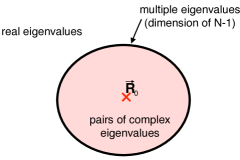
Figure 4: In the neighbourhood of any given geometry $\vec{R}_{0}$, for which a complex energy value is found, pairs of complex eigenvalues occur. Since real eigenvalues exist at some distance from $\vec{R}_{0}$, there is an enveloping space of dimension $N-1$, where multiple eigenvalues arise.

III.3 Shape of conical intersections

For the shape of conical intersections the following is known so far. On the one hand, if the matrix $\bar{H}_{\mathrm{P}}$ is non-defective at the intersection point, the energy gap between the two states in the neighbourhood of the intersection point is linear with the distance from the intersection pointKjønstad et al. (2017) as required by quantum mechanics.Teller (1937) On the other hand, if the $\bar{H}_{\mathrm{P}}$ matrix is defective, numerical investigationsKöhn and Tajti (2007); Kjønstad et al. (2017); Kjønstad and Koch (2017) show a root-like behaviour of the potential surface. In previous investigations both aspects were considered separately and the root-like behaviour was observed but not rationalized by means of a detailed theoretical analysis. With the results from Section II both aspects can be derived mathematically at the same time:

Let us assume that the entries of $\bar{H}_{\mathrm{P}}$ depend analytically on the geometrical parameters of the molecule, since the Hamiltonian depends analytically on the internal coordinates. Varying a given geometry $\vec{R}_{1}$ in one direction thus can be described by a real parameter $r$. The corresponding energy values are determined by the eigenvalues $\lambda_{i}(r)$ of the matrix $\bar{H}_{\mathrm{P}}(r)$. Let us assume furthermore that at a geometry $\vec{R}_{1}$ an intersection occurs, which means that $\lambda(0)$ is a multiple eigenvalue of $\bar{H}_{\mathrm{P}}(0)$. The shape of the conical intersection at $\vec{R}_{1}$ is determined by the eigenvalues $\lambda_{i}(r)$, and depends on the properties of the matrix $\bar{H}_{\mathrm{P}}(0)$:

• In case of a defective matrix $\bar{H}_{\mathrm{P}}(0)$, according to Theorem II.2, the series expansion of the eigenvalue $\lambda(r)$ starts in certain cases with a term proportional to $r^{\frac{1}{2}}$. This leads to a square-root-like evolution of the potential surface close to the intersection seam and to complex eigenvalues near the intersection point.
  

• In case of a non-defective matrix $\bar{H}_{\mathrm{P}}(0)$, according to Theorem II.3, the series expansion of the eigenvalue $\lambda(r)$ near the intersection point starts with a term proportional to $r$. By subtracting the expansions of two eigenvalues

  $$\lambda_{1}(r)=\lambda(0)+a_{1}r+a_{2}r^{1+\frac{1}{\tilde{m}_{1}}}+\cdots,$$

  $$\lambda_{2}(r)=\lambda(0)+b_{1}r+b_{2}r^{1+\frac{1}{\tilde{m}_{2}}}+\cdots$$

  with $\tilde{m}_{1},\tilde{m}_{2}\in\mathbb{N}$, $\tilde{m}_{1}\geq 1,\tilde{m}_{2}\geq 1$, the linearity of the energy gap is obvious:

  $$\lambda_{1}(r)-\lambda_{2}(r)=(a_{1}-b_{1})r+\cdots.$$

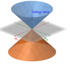
(a) Qualitatively correct shape of a conical intersection, as expected from an EOM-CCSD calculation with a non-defective matrix $\bar{H}_{\mathrm{P}}$.

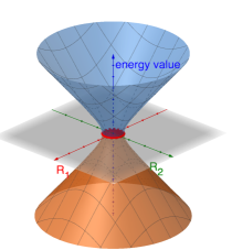
(b) Qualitatively wrong shape of a conical intersection, as it may occur in an EOM-CCSD calculation with a defective matrix $\bar{H}_{\mathrm{P}}$.

Figure 5: Comparison between the shape of a conical intersection in case of a defective and a non-defective matrix $\bar{H}_{\mathrm{P}}$ for a system with two degrees of freedom $R_{1}$ and $R_{2}$.

Figure 5 illustrates the expected behaviour of the potential surfaces in the case of two degrees of freedom for a defective and non-defective matrix. Case $(a)$ shows the correct shape of the potential surface. The dimension of the intersection seam is zero ($N-2$). The linear behaviour close to the intersection point is also clearly visible. A possible shape for the case of a defective matrix is shown in 5 $(b)$. Within the red-coloured disk, pairs of complex-conjugated eigenvalues occur. In the enveloping space, located at the edge of the disk multiple eigenvalues occur. Looking at a cut through this figure, the root-like behaviour along each direction becomes clear. Here all $\bar{H}_{\mathrm{P}}$ matrices based on the molecular geometries located at the edge of the disc are defective.

At this point the question arises in which cases the matrix becomes defective. For the case that the eigenvectors describe crossing states of different symmetries, they cannot become linearly dependent. Assuming that none of the other eigenvalues coincide at this point the matrix is non-defective. In the absence of a constraint that ensures linear independence of the eigenvectors, the defectiveness of the matrix seems to be rather the rule than the exception for the following reasons: First, in general, to ensure a non-defective matrix with multiple eigenvalues more conditions have to be fulfilled than for a defective one.Keller (2008) Second, in numerical examples providing crossing states of the same symmetry defective matrices occur in all cases.Köhn and Tajti (2007); Kjønstad et al. (2017)

On one hand, to avoid defectiveness of the similarity transformed Hamiltonian matrix, symmetric methods (i.e., those derived in the algebraic diagrammatic constructionSchirmer (1982) or unitary CC contextsWatts et al. (1989); Liu et al. (2018b); Grazioli and Stopkowicz (2021)) can be used. On the other hand, a recent paperKjønstad and Koch (2017) suggests to ensure non-defectiveness by including additional constraints in the CC equations.

III.4 Comparison to the two-state model

In the literature,Hättig (2005); Köhn and Tajti (2007); Kjønstad et al. (2017) the behaviour of CC methods at conical intersections has been analyzed using a two-state model. The behaviour in the vicinity of conical intersections is there discussed using the $2\times 2$ matrix $H^{2\times 2}(\vec{R})$ with $\vec{R}$ specifying the molecular geometry near the intersection point $\vec{R}_{0}$. From a mathematical point of view this is justified because the solution of

$$H^{2\times 2}(\vec{R})\vec{v}(\vec{R})=\lambda(\vec{R})\vec{v}(\vec{R})$$ (16)

provides under certain conditions a first-order approximation of the entire eigenvalue problem

$$\bar{H}_{P}(\vec{R})\vec{v}(\vec{R})=\lambda(\vec{R})\vec{v}(\vec{R}).$$ (17)

Assuming that the entries of $\bar{H}_{P}(\vec{R})$ depend analytically on $\vec{R}$ and that $\bar{H}_{P}(\vec{R}_{0})$ is non-defective this can be proven analogously to the CI case.Zhu and Yarkony (2016) In the two-state model, $H^{2\times 2}(\vec{R})$ has the form

$$H^{2\times 2}(\vec{R})=\begin{pmatrix}H_{11}(\vec{R})&H_{12}(\vec{R})\\ H_{21}(\vec{R})&H_{22}(\vec{R})\\ \end{pmatrix}.$$ (18)

The eigenvalues for a given geometry $\vec{R}$ are

$$\lambda_{1,2}=\frac{1}{2}(H_{11}+H_{22})\pm X,$$ (19)

with

$$X=\frac{1}{2}\sqrt{(H_{11}-H_{22})^{2}+4H_{12}H_{21}}.$$ (20)

By means of a detailed analysis of the eigenvalues and eigenvectors of the matrix ${H}^{2\times 2}$ several conclusions have been drawn.Hättig (2005); Köhn and Tajti (2007); Kjønstad et al. (2017) For these conclusions, it should be noted that the model is simply a first-order approximation to the problem and that higher-order effects are not captured. Based on the two-state model the crossing conditions of a conical intersection in a CC calculation were derived leading to the conclusion that for a non-defective ${H}^{2\times 2}$ matrix the dimension of the intersection seam is $N-2$ even if the matrix is not symmetric. This result was not obtained in our analysis of the entire matrix. Based on the existing mathematical literature,Keller (2008) it is however likely that it holds for the entire matrix as well. Both by analysis using the two-state modelKjønstad et al. (2017) as well as by analyzing the entire matrix (as done in the previous section) an energy gap near the intersection point is found that linearly depends on the distance to the intersection. In addition, our analysis of the entire matrix explains the square-root-like behavior of the potential surface in the case of a defective matrix. The latter is not possible by using the two-state model alone since the model does not actually hold for the case of a defective matrix.Zhu and Yarkony (2016)

IV Complex values in case of complex-valued $\bar{H}_{\mathrm{P}}$ matrix

We now turn to the case for which the matrix representation $\bar{H}_{\mathrm{FCI}}$ of the Hamiltonian in the FCI space has complex-valued entries. The decisive difference for the eigenvalues of a complex matrix in contrast to a matrix with only real entries is that complex eigenvalues do not have to occur in pairs. As a consequence of non-pairwise complex eigenvalues a real eigenvalue can gain an imaginary part through an analytic perturbation of the matrix entries without a multiple eigenvalue occurring in between. This is not possible for matrices with only real entries since then Theorem II.5 applies. This leads to the following important statement:
In case of a complex Hamiltonian matrix $\bar{H}_{\mathrm{P}}$ for each energy value (even ground-state energies) of the CC methods an imaginary part may occur, even if the state level is well isolated from other states.

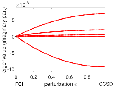
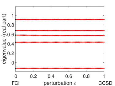
Figure 6: Connection between FCI and CCSD eigenvalues for a complex-valued sample matrix $\bar{H}_{2}$ of the 6-state model.

The connection between FCI eigenvalues and CCSD eigenvalues established in Section III.1 also applies to matrices with complex matrix entries. A sample calculation with a given complex-valued Hamilton matrix $H_{\mathrm{FCI}}$ (see Appendix B) illustrates the continuous transition from FCI eigenvalues to CCSD eigenvalues for the 6-state model (see Section III.1, see Figure 6). Here only the FCI eigenvalues are real. As soon as $\varepsilon$ is non-zero, complex eigenvalues occur. The CCSD eigenvalues are also complex.
The imaginary part of the CCSD eigenvalues is in all cases approximately of the same order of magnitude as the difference between the real parts of the FCI and CCSD eigenvalues (see Table 3). The behaviour of the imaginary part of the eigenvalues of $H_{\mathrm{P}}(\varepsilon)$ is very similar to the development of the deviation of the real parts from the FCI reference (see Figure 7). Analogous to the always existing deviation between the real part of FCI eigenvalues and CCSD eigenvalues, the occurring imaginary part can be considered a kind of "numerical inaccuracy" of the EOM-CCSD method. Therefore, if the EOM-CC method provides a good approximation to the FCI values and the imaginary part is sufficiently small, a meaningful energy value can be defined via the real part of the corresponding CCSD eigenvalue.

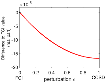
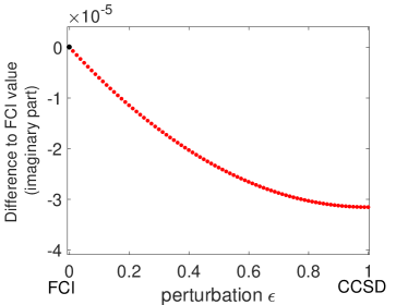
Figure 7: Development of the difference between FCI and CCSD ground-state energy values for the 6-state model. The resulting error behaves in a similar way for both the real and the imaginary parts of the energy differences.

IV.1 Complex energy values for molecules in a strong magnetic field

In the context of CC theory, complex entries in the Hamiltonian matrix $\bar{H}_{\mathrm{P}}$ arise for example due to the presence of a magnetic fieldStopkowicz et al. (2015); Hampe and Stopkowicz (2017) as well as in relativistic quantum-chemical calculations considering spin-orbit coupling.Cowan and Griffin (1976); Saue and Visscher (2003); Berning et al. (2000) In the case of a magnetic field the corresponding literatureStopkowicz et al. (2015); Hampe and Stopkowicz (2017, 2019); Hampe et al. (2020) has so far not reported complex energy values. Nevertheless, complex energy values can indeed occur in finite magnetic-field calculations. We verify this by CCSD calculations for the ground-state of the $\mathrm{H_{2}O}$ molecule in a strong magnetic field.

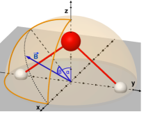
(a) Orientation of the magnetic field vector $\vec{B}$ in the water molecule.

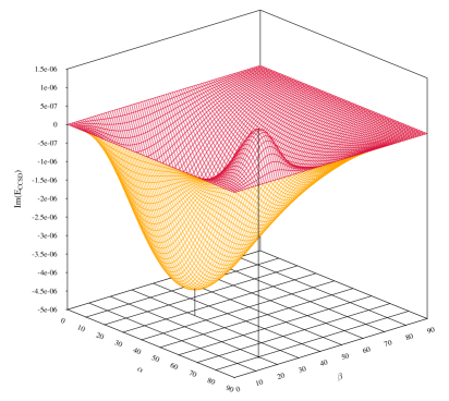
(b) Imaginary part of ground-state energy as results of a CCSD calculation for a water molecule in a strong magnetic field.

Figure 8: Results of CCSD calculations for a water molecule in a strong magnetic field of $0.5$ $\mathrm{B_{0}}$ as a function of the orientation of the magnet-field vector $\vec{B}$.

For the calculations the water molecule is placed in $yz$ plane with the $C_{2}$ axis chosen as the $z$ direction. The alignment of the magnetic field vector $\vec{B}$ is controlled by varying the angles $\alpha$ and $\beta$ from $0^{\circ}$ to $90^{\circ}$ (see Figure 8 $(a)$):

$$\vec{B}(\alpha,\beta)=0.5\begin{pmatrix}\sin(\beta)\\ -\sin(\alpha)\cos(\beta)\\ \cos(\alpha)\cos(\beta)\\ \end{pmatrix}.$$

The bonding angle for the water molecule is chosen to $102.21^{\circ}$ and the bond length to $0.9644$ $\mathrm{\mathring{A}}$. We used a magnetic field of $0.5$ $\mathrm{B_{0}}$ (in this case magnetic and Coulomb forces are of similar magnitude), an uncontracted aug-cc-pVTZ Cartesian basis set Kendall and Dunning Jr. (1992) and gauge-including atomic orbitals.London (1937); Tellgren et al. (2012) The calculations were performed with the QCumbre codeHampe and Stopkowicz (2017); Hampe et al. for the CC part interfaced to the program package LondonTellgren et al. (2008, ) for integral evaluation and the HF part.
The results of the calculation are shown in figure 8. The largest absolute value for the imaginary part of the energy value occurs for angles $\alpha\approx 33^{\circ}$ and $\beta\approx 30^{\circ}$ and amounts to $4\cdot 10^{-6}\mathrm{Hartree}$. The correlation energy in this case is $3\cdot 10^{-1}\mathrm{Hartree}$. This value is about 100.000 times larger than the corresponding imaginary part. Moreover, it is noted that the obtained energy value is real if at least one component of the magnetic-field vector $\vec{B}$ vanishes. This observation is also made in earlier numerical studies.Stopkowicz et al. (2015); Hampe and Stopkowicz (2017, 2019); Hampe et al. (2020) The fact that in these cases real energy values are obtained although the matrix has complex entries suggests that for all these cases a transformation to a real $\bar{H}_{P}$ matrix exists based on symmetry arguments.

Symmetry-inspired transformation to a real $\bar{H}_{\mathrm{P}}$ matrix
We now provide such a symmetry-inspired transformation that yields a real $\bar{H}_{\mathrm{P}}$ matrix for the H₂O molecule following ideas first presented by Pitzer and Winter.Pitzer and Winter (1987)
Let the water molecule with $C_{2v}$ symmetry be placed in the $yz$ plane as in our calculations at the beginning of this section (see Figure 8 (a)). Let us furthermore assume that the CC calculations are performed with real-valued, symmetry-adapted basis functions $\chi$. Let $\boldsymbol{\chi}_{S}$ denote the set of symmetry-adapted basis functions of an arbitrary point-group symmetry $S$, thereby ignoring the applied finite magnetic field (i.e., the point group used for water is then $C_{2v}$). The following unitary transformation will necessarily lead to a real representation of $H_{\mathrm{P}}$: the set of the transformed basis functions $\tilde{\boldsymbol{\chi}}_{S}$ is obtained by taking either the basis functions $\boldsymbol{\chi}_{S}$ in their original form or by multiplying the basis functions of $\boldsymbol{\chi}_{S}$ with $i$. Detailed instruction which of the sets of the basis functions need to be multiplied by $i$ are given in Table 1.

Let $\tilde{\chi}_{\nu}$, $\tilde{\chi}_{\sigma}$, $\tilde{\chi}_{\mu}$ and $\tilde{\chi}_{\rho}$ be the transformed basis functions. Let us now show that with the transformation described above all relevant integrals are real:

1. The one-electron integrals $\bra{\tilde{\chi}_{\nu}}\hat{h}\ket{{\tilde{\chi}_{\mu}}}$, where $\hat{h}$ is the one-electron operator including the kinetic-energy operator, the electron-nucleus repulsion, and the diamagnetic contribution due to the magnetic field.
   This integral does not vanish if and only if $\tilde{\chi}_{\mu}$ and $\tilde{\chi}_{\nu}$ are part of the irreducible representation of the point group $S$. For these cases the integral is always real.

2. The one-electron integrals

   $$\langle\tilde{\chi}_{\mu}|B_{x}\hat{l}_{x}+B_{y}\hat{l}_{y}+B_{z}\hat{l}_{z}|\tilde{\chi}_{\nu}\rangle.$$ (21)

   Here it is important to assume that one component of the magnetic field vanishes. As an example we consider the case $B_{x}=0$. The other cases can be treated in an analogous manner. For the not vanishing integrals $\bra{\tilde{\chi}_{\nu}}B_{y}\hat{l}_{y}\ket{{\tilde{\chi}_{\mu}}}$ and $\bra{\tilde{\chi}_{\nu}}B_{z}\hat{l}_{z}\ket{{\tilde{\chi}_{\mu}}}$, exploitation of the symmetry relations leads to the following finding: The integrals do not vanish if and only if $\tilde{\chi}_{\mu}$ is a real and $\tilde{\chi}_{\nu}$ is an purely imaginary basis function or vice versa. Since $\hat{l}$ includes a $i$, the integrals are real.

3. The two-electron integrals

   $$\bra{\tilde{\chi}_{\nu}\tilde{\chi}_{\sigma}}\ket{{\tilde{\chi}_{\mu}\tilde{\chi}_{\rho}}}.$$ (22)

   Here the combinations of the basic functions from the various irreducible representations must be checked. It turns out that for each possibility either the integral vanishes due to symmetry relations or the integral is real since 0, 2, or 4 of the basis functions $\tilde{\chi}_{\nu}$, $\tilde{\chi}_{\sigma}$, $\tilde{\chi}_{\mu}$ and $\tilde{\chi}_{\rho}$ are imaginary.

The circumstance that all three different types of integrals are real leads to the following conclusions: First, the Fock matrix has only real entries and the molecular orbital coefficients during the HF calculation are real. Second, the two-electron integrals in the molecular-orbital representation are real and the matrix representation $H_{\mathrm{FCI}}$ is thus real as well. Third, a CC calculation provides real amplitudes (see Section II.2). Altogether it can be stated that the $\bar{H}_{\mathrm{P}}$ matrix, which is based on the transformed basis set, has only real entries. Since the eigenvalues remain unchanged under the discussed basis transformation, the energy values even in case of a calculation without application of the basis transformation are real.

Table 1: Transformation of the symmetry-adapted basis functions $\chi$ for water (molecular point group is $C_{2v}$) that leads to a real $H_{\mathrm{P}}$ matrix in case that one component of the magnetic-field vector vanishes.

	$\tilde{\boldsymbol{\chi}}_{A_{1}}$	$\tilde{\boldsymbol{\chi}}_{A_{2}}$	$\tilde{\boldsymbol{\chi}}_{B_{1}}$	$\tilde{\boldsymbol{\chi}}_{B_{2}}$
$B_{x}=0$	$\boldsymbol{\chi}_{A_{1}}$	$i\cdot\boldsymbol{\chi}_{A_{2}}$	$i\cdot\boldsymbol{\chi}_{B_{1}}$	$\boldsymbol{\chi}_{B_{2}}$
$B_{y}=0$	$\boldsymbol{\chi}_{A_{1}}$	$i\cdot\boldsymbol{\chi}_{A_{2}}$	$\boldsymbol{\chi}_{B_{1}}$	$i\cdot\boldsymbol{\chi}_{B_{2}}$
$B_{z}=0$	$\boldsymbol{\chi}_{A_{1}}$	$\boldsymbol{\chi}_{A_{2}}$	$i\cdot\boldsymbol{\chi}_{B_{1}}$	$i\cdot\boldsymbol{\chi}_{B_{2}}$

However, in case of finite magnetic-field calculations GIAOs are usually used. Here the proof, that real energy values are obtained if one component of the magnetic-field vector vanishes is similar, but the proof that the integrals are real is more involved. This can be seen in Appendix C.

IV.2 Complex entries in case of spin-orbit coupling

Finally, we mention the case of relativistic quantum-chemical calculations with inclusion of spin-orbit coupling. This situation is very similar to that of a molecule in a magnetic field. In most methods with spin-orbit coupling Cowan and Griffin (1976); Saue and Visscher (2003); Berning et al. (2000) the expression of the Hamiltonian operator in second quantization equals the known representation from Eq. (4). Then, analogously to the case of the presence of a finite magnetic field, the matrix elements $g$ and $h$ may be complex-valued and the CC equations have the same form as in Eq. (10). The EOM-CCSD energy values are determined via the eigenvalues of $\bar{H}_{\mathrm{P}}$ as described in Section II.2. The matrix $\bar{H}_{\mathrm{P}}$ has complex entries, which may lead to complex energy values.
Similar to finite magnetic-field calculations, a transformation to a real $H_{\mathrm{FCI}}$ matrix may exist in case of point-group or time-reversal symmetry. This has been, for example, shown for some quantum-chemical methodsVisscher (1996); Pitzer and Winter (1987) provided the molecular point group is $C_{2v}$, $D_{2}$ or one of its subgroups. Real energy values for the specified cases are in this way ensured, though in the absence of symmetry complex energy values are expected to be the normal case.

V Concluding remarks

Until now, complex energy values have rarely been observed in CC calculations. This is not surprising, since we are showing in this paper that in standard CC calculations (i.e., those with real-valued Hamiltonian matrices) no complex energy values can occur for the ground state (see section III.1).
In EOM-CC calculations, complex energy values are expected in the vicinity of conical intersections, as already mentionedHättig (2005) and observed Köhn and Tajti (2007); Kjønstad et al. (2017) in the literature. However, complex energy values only appear as long there is no constraint (e.g., due to symmetry) that ensures that the effective Hamiltonian matrix is non-defective. If complex energy values occur, they must be handled with care, since they come with unwanted consequences. First of all they lead to a wrong dimension for the intersection seam (see Section III.2). Furthermore, they lead to a wrong shape of the potential surface in the vicinity of the intersection (see Section III.3). Here we can mathematically deduce the root-like behaviour, which first was observed by Köhn and Tajti.Köhn and Tajti (2007) Along the way, we get evidence that the potential surface shows a linear dependence on the geometrical parameters near the intersection in the case of a non-defective matrix which is consistent with the results from Koch and co-workers.Kjønstad et al. (2017) One last unwanted consequence of complex energy values is the relatively large inaccuracy compared to the FCI solution. We have explained this finding theoretically and observed it in sample calculations for the 6-state-model.

In the case of complex-valued entries in the matrix representation of the Hamiltonian, as they occur in finite magnetic-field CC and relativistic CC calculations with consideration of spin-orbit coupling, we have shown based on mathematical arguments that complex energy values can occur even if the state is well isolated and no conical intersection point lies nearby. By performing calculations for a $\mathrm{H_{2}O}$ molecule in a strong magnetic field we have confirmed this finding.
Due to the established connection between FCI and CCSD energy values (see Section III.1) the appearing imaginary part in many cases can be considered as a kind of "numerical inaccuracy". Therefore the real part of the complex energy value provides a meaningful approximation to the exact energy value, as long as the CCSD method provides a good approximation to the FCI method and the imaginary part is sufficiently small.
The fact that the previous literature did neither report complex energy values for finite magnetic-field CC calculationsStopkowicz et al. (2015); Hampe and Stopkowicz (2017, 2019); Hampe et al. (2020) nor for CC calculations with inclusion of spin-orbit couplingWang et al. (2008); Liu et al. (2018a); Asthana et al. (2019) is explained by our finding that symmetry might offer the possibility to transform the complex $\bar{H}_{\mathrm{FCI}}$ matrix into a real representation.

Appendix A Mathematical proofs

At this point we provide the mathematical proofs for some of the statements used in Section II.1.

Lemma A.1.

Let $U(0)$ be a neighbourhood of $0$ in the complex plane.
Let $f:U(0)\rightarrow\mathbb{C}$ be an analytical function in $U(0)$ for which holds:

$$f(z)\in\mathbb{R},\hskip 14.22636pt\text{ for all }z\in U(0)\cap\mathbb{R}.$$

The coefficients of the power series of $f$ centered at $0$ are then real.

Proof.

Let $f(z)=p_{0}+p_{1}z+p_{2}z+p_{3}z^{2}+\cdots$ be the series expansion of the analytical function $f$ at the point $0$. For the coefficients $p_{n}$ it then holds that

$$p_{n}=\frac{f^{(n)}(0)}{n!},\hskip 14.22636pt\text{where }n\in\mathbb{N}.$$

Let $z_{0}\in U(0)$ be real. Then, for $n=0$ the function $f$ fulfils

$$f^{(0)}(z_{0}):=f(z_{0})\in\mathbb{R}.$$

according to the assumption above. Using mathematical induction starting from the fact that

$$f^{(n)}(z_{0})=\lim_{\begin{subarray}{c}h\rightarrow 0\\ h\in\mathbb{R}\end{subarray}}\left(\frac{f^{(n-1)}(z_{0})-f^{(n-1)}(z_{0}+h)}{h}\right)\in\mathbb{R},$$

yields the result that the values $f^{(n)}(0)$ are real for all $n\in\mathbb{N}$. Here the assumption $h\in\mathbb{R}$ is permitted, since the limit exists. Thus, all coefficients

$$p_{n}=\frac{f^{(n)}(0)}{n!}$$

are real. ∎

We continue by proving Theorem II.4:

Theorem.

Let $\lambda_{i}(\varepsilon)$ be an eigenvalue of the matrix $A(\varepsilon)\in\mathbb{C}(n\times n)$. Furthermore, let $0<a,b\in\mathbb{R}$ exist, such that $\lambda_{i}(\varepsilon)$ takes a real value for all $\varepsilon\in[-a,0]$ and $\lambda_{i}(\varepsilon)$ takes a complex value for all $\varepsilon\in(0,b]$. Then it holds:

1. In a neighbourhood of $\varepsilon=0$ the eigenvalue $\lambda_{i}(\varepsilon)$ can be represented by a branch of a Puiseux series.

2. For $\varepsilon=0$ a multiple eigenvalue occurs.

Proof.

1. Assume that $\lambda_{i}(\varepsilon)$ has no representation as a branch of a Puiseux series as in Eq. (2). Then, according to Theorem II.2, $\lambda_{i}(\varepsilon)$ can be represented as a power series $\lambda_{i}(\varepsilon)=p_{0}+p_{1}\varepsilon+p_{2}\varepsilon^{2}+p_{3}\varepsilon^{3}+\cdots$, which converges for $\varepsilon\in(-r,r)$.
   Let $U_{r/2}(-\frac{r}{2})$ be the open circular disk with center $-\frac{r}{2}$ and radius $\frac{r}{2}$ in the complex plane. Let us define the analytical function

   $$\Lambda(z):\hskip 5.69046ptU_{r/2}\left(-\frac{r}{2}\right)\rightarrow\mathbb{C},\hskip 5.69046pt$$

   $$\Lambda(z)=p_{0}+p_{1}z+p_{2}z^{2}+p_{3}z^{3}+\cdots,$$

   that coincides with $\lambda_{i}(\varepsilon)$ due to its definition on the interval $(-r,0)$. According to the prerequisite it assumes only real values for all $z\in U_{r/2}(-\frac{r}{2})\cap\mathbb{R}$. Using Lemma A.1, we conclude that the coefficients $p_{i}$ are real.
   For this reason, $\lambda_{i}(\varepsilon)$ for $\varepsilon\in(0,b]$ is real. This is a contradiction to the assumption. Thus statement $a)$ is proven.

2. According to Theorem II.2 the development of each simple eigenvalue $\lambda(\varepsilon)$ can be formulated by a power series. Since the eigenvalue $\lambda(0)$ is represented by a Puiseux series due to statement $a)$ of this theorem, a multiple eigenvalue has to occur for $\varepsilon=0$.

∎

Let us finally prove Theorem II.5.

Theorem.

Let $A(\varepsilon)$ be a matrix with only real entries for all $\varepsilon\in(-r,r)$, then:

• Let $\lambda_{i}(\varepsilon)$ be a complex eigenvalue of $A(\varepsilon)$, then the complex-conjugated value $\lambda^{*}_{i}(\varepsilon)$ is also a complex eigenvalue of $A(\varepsilon)$.

• Let $\lambda_{i}(0)$ be a single real eigenvalue of $A(0)$. Then a neighbourhood $U$ of $(0,\lambda_{i}(0))$ exists, in which $\lambda_{i}(\varepsilon)$ takes only real values.

Proof.

For a matrix with only real entries, the characteristic polynomial has only real coefficients. By applying the fundamental theorem of algebra we obtain the first result.
For the second part let us assume that no neighbourhood of $(0,\lambda_{i}(0))$ exists, where $\lambda_{i}(\varepsilon)$ takes only real values. Then a sequence $\varepsilon_{n}$ with $\varepsilon_{n}\rightarrow 0$ exists, for which all eigenvalues $\lambda_{i}(\varepsilon_{n})$ contain an imaginary part.
According to the first statement the complex-conjugated values ${\lambda_{i}}^{*}(\varepsilon_{n})$ are also eigenvalues of $A(\varepsilon)$. Since the eigenvalues depend on the parameter $\varepsilon$ in a continuous manner, the following holds:

$${\lambda_{i}}(\varepsilon_{n})\rightarrow{\lambda(0)},$$

$${\lambda_{i}}^{*}(\varepsilon_{n})\rightarrow{\lambda(0)},\hskip 14.22636pt\text{where }{\lambda_{i}}^{*}(\varepsilon_{n})\neq{\lambda_{i}}(\varepsilon_{n}).$$

Thus, in any neighborhood of $(0,\lambda(0))$ at least two eigenvalues for the same $\varepsilon$ exist. This is a contradiction to Theorem II.2, which proves this theorem. ∎

Appendix B Computational details for the 6-state model

Here, we provide computational details and additional results for the sample calculations on the 6-state model. In the matrix representation ${H}_{\mathrm{FCI}}$ of the Hamiltonian the counter-diagonal elements vanish due to the Slater-Condon rules. The first entry of ${H}_{\mathrm{FCI}}$ vanishes since the Hartree-Fock energy is subtracted from the diagonal elements. For the case of a real Hamiltonian the following matrix representation was chosen:

$$H_{\mathrm{FCI}}=\left(\scriptsize\begin{matrix}0&0.10&0.15&0.05&0.20&0\\ 0.10&0.50&-0.05&0.30&0&0.20\\ 0.15&-0.05&0.60&0&-0.08&0.05\\ 0.05&0.30&0&0.70&-0.03&0.15\\ 0.20&0&-0.08&-0.03&0.80&0.10\\ 0&0.20&0.05&0.15&0.10&1.50\end{matrix}\right).$$

A CC calculation provides here the amplitudes

$$t_{1}=-0.2092, t_{2}=-0.2579,$$

$$t_{3}=0.0161, t_{4}=-0.2486,$$

which lead to the following EOM-CCSD matrix

$$\bar{H}_{\mathrm{P}}=\left(\scriptsize\begin{matrix}-0.1085&0.1000&0.1500&0.0500&0.2000\\ 0&0.4712&-0.0154&0.2589&0\\ 0&-0.0366&0.6395&0&-0.0389\\ 0&0.2611&0&0.6605&-0.0046\\ 0&0&-0.0411&0.0166&0.8288\\ \end{matrix}\right).$$

As example for a complex-valued Hamiltonian the following matrix representation was chosen:

$$H_{\mathrm{FCI}}=\scriptsize\left(\begin{array}[]{cccccc}0&0.1-0.1i&0.15+0.05i&0.05-0.05i&0.2-0.1i&0\\ 0.1+0.1i&0.5&0.06-0.03i&0.03-0.1i&0&0.2-0.1i\\ 0.15-0.05i&0.06+0.03i&0.6&0&0.03-0.1i&0.05-0.05i\\ 0.05+0.05i&0.03+0.1i&0&0.7&0.06-0.03i&0.15+0.05i\\ 0.2+0.1i&0&0.03+0.1i&0.06+0.03i&0.8&0.1-0.1i\\ 0&0.2+0.1i&0.05+0.05i&0.15-0.05i&0.1+0.1i&1.5\\ \end{array}\right)$$

which leads to the amplitudes

$$t_{1}=-0.1539-0.1980i, t_{2}=-0.1882+0.0643i,$$

$$t_{3}=-0.0624-0.0489i, t_{4}=-0.2109-0.0881i,$$

and to the EOM-CC matrix

$$H_{\mathrm{P}}=\scriptsize\left(\begin{array}[]{cccccc}-0.1231&0.1000-0.1000i&0.1500+0.0500i&0.05-0.05i&0.2-0.1i\\ 0&0.4842+0.0079i&0.0558+0.038i&0.0164-0.0661i&0\\ 0&0.0574+0.0109i&0.6259+0.0004i&0&0.0436-0.1339i\\ 0&0.0139+0.0749i&0&0.6741-0.0004&0.0642-0.638i\\ 0&0&0.0461+0.1251i&-0.0008+0.0090i&0.0015-0.0681i\\ \end{array}\right)$$

The eigenvalues for the two examples are given in Table 2 and Table 3.

Table 2: Comparison for the FCI and CCSD eigenvalues of the chosen example real Hamiltonian.

CCSD	FCI	Difference between real part	Difference between imaginary part
eigenvalues	eigenvalues	of CCSD eigenvalues	of CCSD eigenvalues
		and FCI eigenvalues	and FCI eigenvalues
$-0.1085$	$-0.1085$	$8.24\text{\times}{10}^{-06}$	$0$
$0.2881$	$0.2876$	$5.59\text{\times}{10}^{-04}$	$0$
$0.6317$	$0.6290$	$2.69\text{\times}{10}^{-03}$	$0$
$0.8401+0.0049i$	$0.8269$	$1.32\text{\times}{10}^{-02}$	$4.93\text{\times}{10}^{-03}$
$0.8401-0.0049i$	$0.8601$	$-2.00\text{\times}{10}^{-02}$	$-4.93\text{\times}{10}^{-03}$
–	$1.6050$	–	–

Table 3: Comparison for the FCI and CCSD eigenvalues of the chosen example complex Hamiltonian.

CCSD	FCI	Difference between real part	Difference between imaginary part
eigenvalues	eigenvalues	of CCSD eigenvalues	of CCSD eigenvalues
		and FCI eigenvalue	and FCI eigenvalue
$-0.1232-$3.16\text{\times}{10}^{-05}$i$	$-0.1230$	$-1.67\text{\times}{10}^{-04}$	$-3.16\text{\times}{10}^{-05}$
$0.4322+$4.61\text{\times}{10}^{-04}$i$	$0.4306$	$1.61\text{\times}{10}^{-03}$	$4.61\text{\times}{10}^{-04}$
$0.5741+$6.90\text{\times}{10}^{-03}$i$	$0.5820$	$-7.97\text{\times}{10}^{-03}$	$6.90\text{\times}{10}^{-03}$
$0.6779+$1.98\text{\times}{10}^{-03}$i$	$0.6796$	$-1.68\text{\times}{10}^{-03}$	$1.98\text{\times}{10}^{-03}$
$0.9159-$9.34\text{\times}{10}^{-03}$i$	$0.9133$	$2.51\text{\times}{10}^{-03}$	$-9.34\text{\times}{10}^{-03}$
–	$1.6175$	–	–

Appendix C Transformation to a real representation for H₂O in case of symmetry and GIAOs

In the following it is shown that the symmetry-inspired transformation to a real representation from Section IV.1 is also valid with gauge-including atomic orbitals (GIAOs).London (1937); Tellgren et al. (2012) GIAOs have the form

$$\chi^{GIAO}=e^{-\frac{i}{2c}\vec{B}\times(\vec{R}_{\nu}-\vec{R}_{0})\cdot\vec{r}}\chi(\vec{r})$$ (23)

with $c$ as the velocity of light, $\vec{B}$ the magnetic-field vector, $\vec{R_{\nu}}$ the coordinates of $\nu$-th nucleus, $\vec{R}_{0}$ the gauge origin (in the following set to the origin of the coordinate system), $\chi$ the standard real basis function, and $\vec{r}$ the coordinates of the electron.

GIAOs of the water molecule
Let the water molecule be placed in the $yz$ plane as described in Section IV.1 with the oxygen atom at the origin of the coordinate system and $\pm y_{H}$ and $z_{H}$ the coordinates of the two hydrogen atoms. The (non-symmetry-adapted) GIAOs $\chi_{H_{1/2}}^{GIAO}$ of the hydrogen atoms are then given by:

$$\chi_{H_{1/2}}^{GIAO} =e^{-\frac{i}{2c}\left(\begin{pmatrix}B_{x}\\ B_{y}\\ B_{z}\\ \end{pmatrix}\times\begin{pmatrix}0\\ \pm y_{H}\\ z_{H}\\ \end{pmatrix}\right)\cdot\begin{pmatrix}x\\ y\\ z\\ \end{pmatrix}}\chi_{H_{1/2}}.\hskip 14.22636pt$$ (24)

A Taylor expansion of the exponential up to second order yields

$$\chi_{H_{1/2}}^{GIAO}= \chi_{H_{1/2}}-\frac{i}{2c}\pm y_{H}(B_{x}z-B_{z}x)\chi_{H_{1/2}}$$

$$-\frac{i}{2c}z_{H}(B_{y}x-B_{x}y)\chi_{H_{1/2}}$$

$$-0.5(\frac{1}{2c}y_{H})^{2}(\pm B_{x}z\mp B_{z}x)^{2}\chi_{H_{1/2}}$$

$$-(\frac{1}{2c})^{2}(\pm y_{H})z_{H}(B_{x}z-B_{z}x)$$

$$\qquad\qquad(B_{y}x-B_{x}y)\chi_{H_{1/2}}$$

$$+0.5(\frac{1}{2c}z_{H})^{2}(B_{y}x-B_{x}y)^{2}\chi_{H_{1/2}}$$

$$+\cdots$$ (25)

Note that due to our choice of the coordinate system the GIAOs of the oxygen atom are identical to the corresponding AOs.

Symmetry adaptation then leads to the following second-order expression for the symmetry-adapted hydrogen GIAOs:

$$\chi_{H_{\pm}}^{GIAO}= \chi_{H_{1}}^{GIAO}\pm\chi_{H_{2}}^{GIAO}$$

$$= (\chi_{H_{1}}\pm\chi_{H_{2}})$$

$$-\frac{i}{2c}y_{H}(B_{x}z-B_{z}x)(\chi_{H_{1}}\mp\chi_{H_{2}})$$

$$-\frac{i}{2c}z_{H}(B_{y}x-B_{x}y)(\chi_{H_{1}}\pm\chi_{H_{2}})$$

$$-0.5(\frac{1}{2c}y_{H})^{2}(-B_{x}z+B_{z}x)^{2}(\chi_{H_{1}}\pm\chi_{H_{2}})$$

$$-(\frac{1}{2c})^{2}y_{H}z_{H}(B_{x}z-B_{z}x)$$

$$\qquad\qquad(B_{y}x-B_{x}y)(\chi_{H_{1}}\mp\chi_{H_{2}})$$

$$-0.5(\frac{1}{2c}z_{H})^{2}(B_{y}x-B_{x}y)^{2}(\chi_{H_{1}}\pm\chi_{H_{2}})$$

$$+\cdots$$ (26)

Symmetry classification of real and imaginary part
It is now rather straightforward to see that the real and imaginary terms in the expansion belong to different irreducible representations provided one magnetic-field component vanishes (see Table 4). For example, in case of $B_{x}=0$, the real contributions in the expansion are of $A_{1}$ and $B_{2}$ symmetry for AOs of $A_{1}$ and $B_{2}$ symmetry, while the imaginary terms are of $B_{1}$ and $A_{2}$ symmetry. For AOs of $B_{1}$ and $A_{2}$ symmetry, the situation is reversed and the real terms are of $B_{1}$ and $A_{2}$ symmetry, while the imaginary contributions are of $A_{1}$ and $B_{2}$ symmetry. This observation suggests that the unitary transformation introduced in Section IV.1 provides a consistent representation in which all real contributions are of $A_{1}$ and $B_{2}$ symmetry and all imaginary contributions are of $B_{1}$ and $A_{2}$ symmetry. The proof that this unitary transformation provides a real representation of all relevant one- and two-electron integrals as well of the Hamiltonian matrix is then analogous to the one given in Section IV.1. For the cases in which one of the other magnetic-field components vanishes, the proof can be carried out in an similar manner with grouping $A_{1}$ and $B_{1}$ as well as $B_{2}$ and $A_{2}$ symmetries together in case of $B_{y}=0$ and $A_{1}$ and $A_{2}$ as well $B_{1}$ and $B_{2}$ symmetries in the case of $B_{z}=0$.

The proof that in case of symmetry CC calculation for systems in finite magnetic fields can be carried out with real Hamiltonians always holds provided that for the given symmetry-adapted GIAOs the real and imaginary terms belong to different irreducible representations.

Table 4: Symmetry classification of the real and imaginary parts of the GIAOs for water depending on the irreducible representation of the underlying AO.

	symmetry of AO
	A1	B1	B2	A2
a) $B_{x}$=0
real part	A1,B2	A2, B1	A1, B2	B1,A2
imag. part	B1, A2	A1, B2	A2, B1	A1, B2
a) $B_{y}$=0
real part	A1,B1	A1, B1	B2, A2	B2, A2
imag. part	B2, A2	B2, A2	A1, B1	A1, B1
a) $B_{z}$=0
real part	A1, A2	B1, B2	B1, B2	A1, A2
imag. part	B1, B2	A1, A2	A1, A2	B1, B2

References

- Shavitt and Bartlett (2009) I. Shavitt and R. J. Bartlett, Many-Body Methods in Chemistry and Physics (Cambridge University Press, Cambridge, 2009).
- Emrich (1981) K. Emrich, Nucl. Phys. A 351, 379 (1981).
- Stanton and Bartlett (1993a) J. F. Stanton and R. J. Bartlett, J. Chem. Phys. 98, 7029 (1993a).
- Comeau and Bartlett (1993) D. C. Comeau and R. J. Bartlett, Chem. Phys. Lett. 207, 414 (1993).
- Rico and Head-Gordon (1993) R. J. Rico and M. Head-Gordon, Chem. Phys. Lett. 213, 224 (1993).
- Hättig (2005) C. Hättig, Adv. Quant. Chem. 50, 37 (2005).
- Köhn and Tajti (2007) A. Köhn and A. Tajti, J. Chem. Phys. 127, 044105 (2007).
- Kjønstad et al. (2017) E. F. Kjønstad, R. H. Myhre, T. J. Martinez, and H. Koch, J. Chem. Phys. 147, 164105 (2017).
- Stopkowicz et al. (2015) S. Stopkowicz, J. Gauss, K. K. Lange, E. I. Tellgren, and T. Helgaker, J. Chem. Phys. 143, 074110 (2015).
- Hampe and Stopkowicz (2017) F. Hampe and S. Stopkowicz, J. Chem. Phys. 146, 154105 (2017).
- Hampe et al. (2020) F. Hampe, N. Gross, and S. Stopkowicz, Phys. Chem. Chem. Phys. 22, 23522 (2020).
- Visscher et al. (1996) L. Visscher, T. L. Lee, and K. G. Dyall, J. Chem. Phys. 105, 8769 (1996).
- Wang et al. (2008) F. Wang, J. Gauss, and C. van Wüllen, J. Chem. Phys. 129, 064113 (2008).
- Shee et al. (2018) A. Shee, T. Saue, T. Visscher, and A. S. P. Gomes, J. Chem. Phys. 149, 174113 (2018).
- Liu et al. (2018a) J. Liu, Y. Shen, A. Asthana, and L. Cheng, J. Chem. Phys. 148, 034106 (2018a).
- Wilkinson (1965) J. H. Wilkinson, The Algebraic Eigenvalue Problem, revised. ed. (Clarendon Press, Oxford, 1965).
- Kato (1995) T. Kato, Perturbation Theory for Linear Operators (Springer, Berlin Heidelberg, 1995).
- Wall (2004) C. T. C. Wall, Singular Points of Plane Curves (Cambridge University Press, Cambridge, 2004).
- Thomas (2018) S. Thomas, Komplexe Eigenwerte in der Equation-of-Motion Coupled-Cluster-Theorie, Master’s thesis, Johannes Gutenberg-Universität Mainz (2018).
- Golub and Loan (2013) G. H. Golub and C. F. V. Loan, Matrix Computations, 4th ed. (JHU Press, London, 2013).
- Dyall and Fægri Jr. (2007) K. G. Dyall and K. Fægri Jr., Introduction to Relativistic Quantum Chemistry (Oxford University Press, New York, 2007).
- Hampe and Stopkowicz (2019) F. Hampe and S. Stopkowicz, J. Chem. Theory Comput. 15, 4036 (2019).
- Bartlett and Musiał (2007) R. J. Bartlett and M. Musiał, Rev. Mod. Phys. 79, 291 (2007).
- Schneider (2009) R. Schneider, Numerische Mathematik 113, 433 (2009).
- Purvis III and Bartlett (1982) G. D. Purvis III and R. J. Bartlett, J. Chem. Phys. 76, 1910 (1982).
- Rowe (1968) D. J. Rowe, Rev. Mod. Phys. 40, 153 (1968).
- Stanton and Bartlett (1993b) J. F. Stanton and R. J. Bartlett, J. Chem. Phys. 98, 7029 (1993b).
- Kowalski and Piecuch (2001) K. Kowalski and P. Piecuch, J. Chem. Phys. 115, 643 (2001).
- Kucharski et al. (2001) S. A. Kucharski, M. Włoch, M. Musiał, and R. J. Bartlett, J. Chem. Phys. 115, 8263 (2001).
- Bomble et al. (2004) Y. J. Bomble, K. W. Sattelmeyer, J. F. Stanton, and J. Gauss, J. Chem. Phys. 121, 5236 (2004).
- Kállay and Gauss (2004) M. Kállay and J. Gauss, J. Chem. Phys. 121, 9257 (2004).
- Yarkony (1996) D. R. Yarkony, Rev. Mod. Phys. 68, 985 (1996).
- Matsika and Yarkony (2001) S. Matsika and D. R. Yarkony, J. Chem. Phys. 115, 2038 (2001).
- Truhlar and Mead (2003) D. G. Truhlar and C. A. Mead, Phys. Rev. A 68, 032501 (2003).
- Zhu and Yarkony (2016) X. Zhu and D. R. Yarkony, Mol. Phys. 114, 1983 (2016).
- von Neuman and Wigner (1929) J. von Neuman and E. Wigner, Physik. Z. 30, 467 (1929).
- Keller (2008) J. Keller, Linear Algebra & its Applications 429, 2209 (2008).
- Teller (1937) E. Teller, J. Chem. Phys. 42, 109 (1937).
- Kjønstad and Koch (2017) E. F. Kjønstad and H. Koch, J. Phys. Chem. Lett. 8, 4801 (2017).
- Schirmer (1982) J. Schirmer, Phys. Rev. A 26, 2395 (1982).
- Watts et al. (1989) J. D. Watts, G. W. Trucks, and R. J. Bartlett, Chem. Phys. Lett. 157, 359 (1989).
- Liu et al. (2018b) J. Liu, A. Asthana, L. Cheng, and D. Mukherjee, J. Chem. Phys. 148, 244110 (2018b).
- Grazioli and Stopkowicz (2021) L. Grazioli and S. Stopkowicz, “Unitary coupled cluster theory for atoms and molecules in strong magnetic fields,” (2021), in preparation.
- Cowan and Griffin (1976) R. D. Cowan and D. Griffin, J. Opt. Soc. Am. 66, 1010 (1976).
- Saue and Visscher (2003) T. Saue and L. Visscher, in Theoretical Chemistry and Physics of Heavy and Superheavy Elements, edited by U. Kaldor and S. Wilson (Kluwer Academic Publishers, Dordrecht, 2003) p. 211.
- Berning et al. (2000) A. Berning, M. Schweizer, H.-J. Werner, P. J. Knowles, and P. Palmieri, Mol. Phys. 98, 1823 (2000).
- Kendall and Dunning Jr. (1992) R. A. Kendall and T. H. Dunning Jr., J. Chem. Phys. 96, 6796 (1992).
- London (1937) F. London, J. Phys. Radium 8, 397 (1937).
- Tellgren et al. (2012) E. I. Tellgren, S. S. Reine, and T. Helgaker, Phys. Chem. Chem. Phys. 14, 9492 (2012).
- (50) F. Hampe, S. Stopkowicz, N. Gross, and M.-P. Kitsaras, “QCUMBRE, Quantum8-Chemical Utility enabling Magnetic-field dependent investigations Benefiting from Rigorous Electron-correlation treatment,” qcumbre.org.
- Tellgren et al. (2008) E. I. Tellgren, A. Soncini, and T. Helgaker, J. Chem. Phys. 129, 154114 (2008).
- (52) E. I. Tellgren, T. Helgaker, A. Soncini, K. K. Lange, A. M. Teale, U. Ekström, S. Stopkowicz, J. H. Austad, and S. Sen, “LONDON, a quantum-chemistry program for plane-wave/GTO hybrid basis sets and finite magnetic field calculations,” londonprogram.org.
- Pitzer and Winter (1987) R. M. Pitzer and N. W. Winter, J. Phys. Chem. 92, 3061 (1987).
- Visscher (1996) L. Visscher, Chem. Phys. Lett. 253, 20 (1996).
- Asthana et al. (2019) A. Asthana, J. Liu, and L. Cheng, J. Chem. Phys. 150, 0074102 (2019).