The effect of phased recurrent units in the classification of multiple catalogs of astronomical lightcurves

Abstract

In the new era of very large telescopes, where data is crucial to expand scientific knowledge, we have witnessed many deep learning applications for the automatic classification of lightcurves. Recurrent neural networks (RNNs) are one of the models used for these applications, and the LSTM unit stands out for being an excellent choice for the representation of long time series. In general, RNNs assume observations at discrete times, which may not suit the irregular sampling of lightcurves. A traditional technique to address irregular sequences consists of adding the sampling time to the network’s input, but this is not guaranteed to capture sampling irregularities during training. Alternatively, the Phased LSTM unit has been created to address this problem by updating its state using the sampling times explicitly. In this work, we study the effectiveness of the LSTM and Phased LSTM based architectures for the classification of astronomical lightcurves. We use seven catalogs containing periodic and nonperiodic astronomical objects. Our findings show that LSTM outperformed PLSTM on 6/7 datasets. However, the combination of both units enhances the results in all datasets.

1 Introduction

Every night, terabytes of photometric data are being collected by wide-field telescopes (Bellm et al., 2018). The amount of data will increase considerably by 2023 when the Vera C. Rubin Observatory will begin operations (Ivezić et al., 2019). These time-domain surveys scan a large portion of the sky, capturing several time-variable phenomena. The data from these variable sources are usually represented as lightcurves that describe underlying astrophysical properties, allowing scientists to identify and label different astronomical objects (Bonanos 2006; Tammann et al. 2008; Pietrzyński 2018). For some astrophysical events, it is crucial to obtain this classification in real-time to promptly follow-up individual targets (Abbott et al. 2017a; Abbott et al. 2017b; Schulze et al. 2018). In this context, human visual inspection is not enough to rapidly label incoming data. During the last decade, many Machine Learning (ML) models have been proposed to speed up the automatic classification of objects.

Classical ML models have been successfully applied in Astronomy for the classification of photometric data (Lochner et al. 2016; Mackenzie et al. 2016; Lochner et al. 2016; Castro et al. 2017; Devine et al. 2018; Bai et al. 2018; Martínez-Palomera et al. 2018; Castro et al. 2018; Fotopoulou & Paltani 2018; Valenzuela & Pichara 2018; Mahabal et al. 2019; Sánchez et al. 2019; Villar et al. 2019; Boone 2019; Zorich et al. 2020; Sánchez-Sáez et al. 2021). These “classical" methods require an initial feature extraction module, in which the scientist defines ad hoc features. This procedure is time-consuming and, depending on the features chosen, it could scale the number of operations significantly, implying a high computational cost. Moreover, the features, obtained by expert knowledge, may be insufficient for the models to learn in certain domains e.g., classifying transients using periodic-based features.

Since 2015, Deep learning (DL) algorithms have been applied to Astronomy and have outperformed many classical ML models (e.g. Dieleman et al. (2015), Gravet et al. (2015); Cabrera-Vives et al. (2017); Mahabal et al. (2017), George & Huerta (2018)). DL methods aim to automatically extract the features needed to perform a particular task, avoiding the feature engineering process (LeCun et al., 2015).

Recently, recurrent neural networks (RNN, Rumelhart et al. 1986) have been applied to classify sequential data such as lightcurves (Charnock & Moss 2017, Moss 2018; Naul et al. 2018; Muthukrishna et al. 2019; Becker et al. 2020; Chaini & Kumar 2020; Neira et al. 2020; Jamal & Bloom 2020) and sequences of astronomical images (Carrasco-Davis et al. 2019, Gómez et al. 2020, Möller & de Boissière 2020). However, most DL models are not ideal for processing lightcurves as they assume regular and discrete sampling, while lightcurves measurements have different cadences in a continuous domain.

In the previous paragraph, most of the works use sampling times within the network’s input to learn time-related features, which may help with the irregularity. However, even when using time as an input, the weight updates remain regular and discrete, regardless of the spacing between observations. Other approaches try to regularize lightcurve times so we can fit the model assumptions. For example, Naul et al. 2018 folds lightcurves to decrease the sampling gaps from the continuous timescale, and Muthukrishna et al. 2019 interpolates observations at 3-day intervals. However, folding lightcurves do not assure eliminating the irregularity because it is still an approximation that depends on the number of measurements. On the other hand, interpolation may break variability patterns that come from the astrophysical properties.

Alternatively, Neil et al. 2016 introduced a novel recurrent unit, called the Phased Long Short Term Memory (PLSTM), an extension of the Long Short Term Memory (LSTM) that incorporates a time gate in charge of considering the effect of irregular sampling on the neural weights updates. We bet on the use of this unit to cover the information lost by the others methods.

In this work, we explore the effectiveness of classifying astronomical time series using both the PLSTM and traditional methods, such as the Long Short Term Memory (LSTM), and a Random Forest trained on features. We test our models using OGLE (Udalski et al. 1997), MACHO (Alcock et al. 1995), ASAS (Pojmanski & Maciejewski 2005), LINEAR (Stokes et al. 2000), Catalina Sky Survey (Drake et al. 2009), Gaia (Collaboration et al. 2016), and WISE (Wright et al. 2010), which are widely-used catalogs containing periodic and non-periodic variable stars. We do not fold the lightcurves for periodical classes because it requires period calculation, which is time-consuming and limits nonperiodical objects’ classification.

We propose the L+P architecture, a new classifier that combines a PLSTM with an LSTM, the later includes sampling times in its input. We compare this model with a Random Forest (RF) trained on features and the state-of-the-art of the mentioned catalogs. Since our model uses unprocessed observations, it is faster to predict and more accurate than the RF when we have lightcurves with less than 20 observations.

This is paper is organized as follows: In Section 2 we provide an overview of the theoretical background of recurrent neural networks, specifically within the context of describing both LSTM and Phased LSTM units. In Section 3, we present the data catalogs used in this work. Section 4 introduces data preprocessing, the architecture of the proposed model, metrics, and model selection. Finally, we show the results and draw the conclusions in sections 5 and 6, respectively.

2 Background

Neural networks (NN) are parametric functions capable of transforming a vector input $\boldsymbol{x}\in\mathbb{R}^{D}$ to an expected target $\boldsymbol{y}$. We will focus on a classification task, where the output consists of one of $K$ classes. Hereafter, we assume $\boldsymbol{y}\in\mathbb{R}^{K}$ is a one-hot encoded vector that is 1 for the actual class and zero otherwise.

A NN comprises neurons that transform the input by multiplying it by a weight matrix $\rm{W}$ and adding a vector of biases $\boldsymbol{b}$. This transformation is passed through an element-wise nonlinear activation function $g$. When training a NN, the goal is to learn $\rm{W}$ and $\boldsymbol{b}$, capturing nonlinear relationships between variables. Equation 1 describes a Fully-Connected (FC) layer which receives $\boldsymbol{x}$ as input,

$$\boldsymbol{h}=g(\mathrm{W}^{\top}\boldsymbol{x}+\boldsymbol{b}),$$ (1)

where $\boldsymbol{h}$ is the layer output. Stacking FC layers increases the classification capacity of the NN by learning features at multiple levels of abstraction (Glorot & Bengio, 2010). In this case, the output of each stacked layer serves as input for the next one. These particular types of neural networks are called multi-layer perceptron (MLP) (Rumelhart et al., 1986).

MLPs have been widely used for regression and classification tasks. Their matrix representation allows fast computation, which can be parallelized on GPU (Oh & Jung, 2004). Usually, MLPs assume that each entry within the input is independent of each other. However, this is not the case of a time series, where the input is a sequence of measurements, and each point may be conditioned on the previous points.

In the following sections we explain the architecture of the recurrent neural network (RNN), an extension of the MLPs capable of learning time-based patterns from data (Section 2.1). We also describe the operation of the LSTM (Section 2.2) and PLSTM (Section 2.3), as they are the two types of recurrent neurons used in this work.

2.1 Recurrent Neural Networks

Recurrent neural networks are capable of learning dependencies on sequential data. They use a hidden state vector $\boldsymbol{h}$ that preserves the information of previous time steps. Formally, a vanilla recurrent unit is given by:

$$\boldsymbol{h}^{(l)}=g{\left(\mathrm{W}^{\top}_{x}\boldsymbol{x}^{(l)}+\mathrm{W}_{h}^{\top}\boldsymbol{h}^{(l-1)}+\boldsymbol{b}\right)},$$ (2)

where $[\mathrm{W}^{\top}_{x}$, $\mathrm{W}^{\top}_{h}]$ are the weights for $x$ the input and $h$ the hidden state at the current ($l$) and previous ($l-1$) time step, respectively. Note the representation is quite similar to an MLP. However, recurrent neurons combine the current observations $\boldsymbol{x}^{(l)}$ with the previous activation (or hidden state) $\boldsymbol{h}^{(l-1)}$ to build the input to the $l$-th layer.

Figure 1a shows a vanilla recurrent neural unit corresponding to Equation 2. Notice that the information flows in the sense of arrows. The arrow bifurcation in the last part of the diagram indicates the potential of the neuron to make predictions while connecting with the next step. In other words, the hidden state $\boldsymbol{h}^{(l)}$ represents a feature vector that describes the time series up to the current step. Usually, RNNs use a FC layer that receives the hidden state to classify new observations,

$$\boldsymbol{\hat{y}^{(l)}}=\text{softmax}(\rm{W_{o}^{\top}}\boldsymbol{h^{(l)}}+\boldsymbol{b}_{o})$$ (3)

where $\rm{W}^{\top}_{o}$ and $\boldsymbol{b}_{o}$ are the weights and biases of the FC layer, and $\boldsymbol{\hat{y}^{(l)}}$ is the predicted label at the $l$-th step.

During the training of RNNs, the gradients flow through the steps of the network. To calculate the gradients, we differentiate the loss function regarding the activation of each time step. Thus, if the gradient is backpropagated until the first time step, as the length of the sequence increases, several matrix multiplications are performed because of the chain rule (Werbos et al., 1990). If at some time in the recurrence, the gradients have low values ($<1$), the total product may vanish. On the other hand, if the values are high ($>1$), the gradient could explode. This problem is known as the exploding and vanishing of the gradient (Pascanu et al., 2012) and is the motivation for creating the Long Short Term Memory (LSTM) recurrent unit.

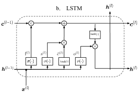
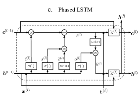
Figure 1: Recurrent neural units. Everything within the dashed line is part of the neuron. The rows represent the flow of information, starting from the inputs ($\boldsymbol{h}^{(l-1)}$ previous hidden and $\boldsymbol{c}^{(l-1)}$ cell state, $\boldsymbol{x}^{(l)}$ current observation and $t^{(l)}$ its sampling time) outside the neuron to the new states ($\boldsymbol{h}^{(l)}$ hidden, and $\boldsymbol{c}^{(l)}$ cell state). Boxes are nonlinear transformation for recurrent gates ($f^{(l)},s^{(l)},o^{(l)},k^{(l)}$) and the candidate state ($c^{(l)}$) with sigmoid ($\sigma(\cdot)$) and hyperbolic tangent ($\tanh(\cdot)$) activation functions respectively.

2.2 Long Short Term Memory (LSTM)

The Long Short Term Memory unit, introduced by Hochreiter & Schmidhuber 1997b, is a recurrent unit capable of learning long-term dependencies from time series. Unlike the vanilla recurrent unit, the LSTM has an additional cell state that scales the neuron’s output according to long-term relevant information stored in it.

Both the LSTM cell ($\boldsymbol{c}^{(l)}$) and the hidden ($\boldsymbol{h}^{(l)}$) state vectors have the same dimensionality, but their values are updated differently. Updates are controlled by recurrent gates, MLPs that receive the current observation and the previous hidden state to learn specific tasks. Typically, the LSTM uses a gate to save ($\boldsymbol{s}^{(l)}$) and another one to forget ($\boldsymbol{f}^{(l)}$) long-term patterns. A third gate ($\boldsymbol{o}^{(l)}$) scales the output of the unit. Formally,

$$\boldsymbol{c}^{(l)}=\boldsymbol{f}^{(l)}\odot\boldsymbol{c}^{(l-1)}+\boldsymbol{s}^{(l)}\odot\boldsymbol{\tilde{c}}$$ (4)

$$\boldsymbol{h}^{(l)}=\boldsymbol{o}^{(l)}\odot\tanh{(\boldsymbol{c}^{(l)})}$$ (5)

where $\odot$ is the Hadamard product of vectors, $\boldsymbol{\tilde{c}}$ is a candidate cell state defined as,

$$\boldsymbol{\tilde{c}}^{(l)}=\tanh{(\rm{W}_{cx}^{\top}\boldsymbol{x}^{(l)}+\rm{W}_{ch}^{\top}\boldsymbol{h}^{(l-1)}+\boldsymbol{b_{c}})}$$ (6)

and

$$\boldsymbol{f}^{(l)}=\sigma(\rm{W}_{fx}^{\top}\boldsymbol{x}^{(l)}+\rm{W}_{fh}^{\top}\boldsymbol{h}^{(l-1)}+\boldsymbol{b_{f}})$$ (7)

$$\boldsymbol{s}^{(l)}=\sigma(\rm{W}_{sx}^{\top}\boldsymbol{x}^{(l)}+\rm{W}_{sh}^{\top}\boldsymbol{h}^{(l-1)}+\boldsymbol{b_{s}})$$ (8)

$$\boldsymbol{o}^{(l)}=\sigma(\rm{W}_{ox}^{\top}\boldsymbol{x}^{(l)}+\rm{W}_{oh}^{\top}\boldsymbol{h}^{(l-1)}+\boldsymbol{b_{o}}).$$ (9)

In this formulation, $[\rm{W}_{fx},\rm{W}_{fh},\boldsymbol{b_{f}}]$, $[\rm{W}_{sx},\rm{W}_{sh},\boldsymbol{b_{s}}]$, and $[\rm{W}_{ox},\rm{W}_{oh},\boldsymbol{b_{o}}]$ are the weights and biases of the forget, save, and output gate, respectively.

Figure 1b. shows the LSTM structure and its operations. The network’s input is formed by the new observations and the previous hidden and cell states, typically initialized to zero.

LSTM signified a breakthrough for long time series analysis in many fields of science (Hochreiter & Schmidhuber 1997a; Greff et al. 2016). However, this unit does not consider irregular sampling times when updating the states in equations 4 and 5. Consequently, it assumes that all step updates weigh the same regardless of how far they are from the last observation.

2.3 Phased Long Short Term Memory (PLSTM)

The Phased Long Short Term Memory proposed by Neil et al. 2016 is an extension of the LSTM unit for processing inputs sampled at irregular times. The idea is to consider sampling times explicitly during the state updates. To do this, the PLSTM assumes the observations come from periodic sampling and, therefore, the neurons should be controlled by independent rhythmic oscillations following these periodicities.

Every neuron in the H-dimensional state has a learnable independent period, forming the vector $\boldsymbol{\tau}\in\mathbb{R}^{H}$. Then, for a given $l$-th step, we calculate the phase of neurons $\boldsymbol{\phi}^{(l)}$ as

$$\boldsymbol{\phi}^{(l)}=\frac{(t^{(l)}-\boldsymbol{s})\ mod\ \boldsymbol{\tau}}{\boldsymbol{\tau}},$$ (10)

where $\boldsymbol{s}\in\mathbb{R}^{H}$ represents the trainable shift of the signal and $t^{(l)}$ is the $l$-th sampling time. PLSTM adds a time gate which is defined as a piece-wise function depending on the phases and a trainable vector $\boldsymbol{\rho}\in\mathbb{R}^{H}$ that controls the duration of the openness phase,

$$\boldsymbol{k}^{(l)}=\begin{cases}\frac{2\boldsymbol{\phi}^{(l)}}{\boldsymbol{\rho}}&if\ \boldsymbol{\phi}^{(l)}<\frac{1}{2}\boldsymbol{\rho}\\ 2-\frac{2\boldsymbol{\phi}^{(l)}}{\boldsymbol{\rho}}&if\frac{1}{2}\boldsymbol{\rho}<\boldsymbol{\phi}^{(l)}<\boldsymbol{\rho}\\ \alpha\boldsymbol{\phi}^{(l)}&otherwise.\end{cases}$$ (11)

In Equation 11 $\alpha$ is a leak parameter close to zero which allows gradient information flow (He et al., 2015) for those cases where the gate is closed. The time gate $k^{(l)}$ controls how much of the proposed states should flow to the next recurrence. Unlike the LSTM, the PLSTM does not consider every update equally important to each other, and therefore, it weighs the updates by using the current sampling time. Using the output of the time gate formulation in Equation 11, we update the cell states in the following way:

$$\hat{\boldsymbol{c}}^{(l)}=\boldsymbol{f}^{(l)}\odot\boldsymbol{c}^{(l-1)}+\boldsymbol{s}^{(l)}\odot\boldsymbol{\tilde{c}}^{(l)}$$ (12)

$$\boldsymbol{c}^{(l)}=\boldsymbol{k}^{(l)}\cdot\boldsymbol{\hat{c}}^{(l)}+(1-\boldsymbol{k}^{(l)})\cdot\boldsymbol{c}^{(l-1)}$$ (13)

$$\hat{\boldsymbol{h}}^{(l)}=\boldsymbol{o}^{(l)}\odot g(\boldsymbol{c}^{(l)})$$ (14)

$$\boldsymbol{h}^{(l)}=\boldsymbol{k}^{(l)}\cdot\boldsymbol{\hat{h}}^{(l)}+(1-\boldsymbol{k}^{(l)})\cdot\boldsymbol{h}^{(l-1)}$$ (15)

where $\boldsymbol{\hat{c}}_{l}$ and $\boldsymbol{\hat{h}}_{l}$ are the candidate states at $l$-th step. Note that if we replace $\boldsymbol{k}^{(l)}=1$, then we get the LSTM output.

For irregular sampled continuous-time sequences, the observation time controls the update of each neuron (see Figure 2), allowing improvements in the convergence ratio as well as the loss minimization.

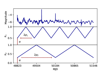
Figure 2: Time gate openness phases controlling the update rate for the states of a single lightcurve. The trainable openness duration $\rho$ depends on a particular neuron, while the leak parameter $\alpha$ is shared across the state. A neuron is fully updated when the curve is in the peak, i.e., $k_{i}=1$. Otherwise, it is partially updated, as described in Equation 11.

The Phased LSTM has also been used for multi-event time series in which independent sequences describe the same phenomena (Anumula et al. 2018; Liu et al. 2018).

3 Data

Our classification domain is composed of variable stars in the form of photometric lightcurves. Each light curve corresponds to a set of observations taken at different times and varies in length depending on the objective of the surveys. In this context, we collected data from seven widely used surveys that we describe as follows:

The Massive Astrophysical Compact Halo Objects (MACHO): The MACHO project (Alcock et al., 2000) results from a collaboration between different institutions to look for dark matter in the halo of the Milky Way. Based on several years of observation, astronomers tried to find the dark matter by its effect on the bright matter. We used the catalog from Kim et al. 2011. Table 1 shows the MACHO dataset composition following the same blue-band selection made by Nun et al. 2014. The objects are principally periodic variable stars except for Quasars (QSO) and Microlensings (MOA).

The Lincoln Near-Earth Asteroid Research (LINEAR):
LINEAR (Stokes et al., 2000) is a collaborative program aiming at monitoring asteroids, founded by the US Air Force and NASA, and has the collaboration of The Lincoln Laboratory at the Massachusetts Institute of Technology. Table 2 shows the training set composition made by Naul et al. 2018, which contains periodical lightcurves measured in $r\leq 18$ red band (see Palaversa et al. 2013 for more details).

The All Sky Automated Survey (ASAS):
With two observation stations, ASAS (Pojmanski & Maciejewski, 2005) is a low-cost project focused on photometric monitoring of the entire sky. A catalog of variable stars constitutes one of the main goals of this project. We use V-band periodical lighcurves selected by Naul et al. 2018. Table 3 describes the number of object per class.

The Optical Gravitational Lensing Experiment (OGLE):
OGLE (Udalski et al., 1997) is an observation project, currently operational (OGLE-IV), that started in 1992 (OGLE-I) under the initiative of the University of Warsaw. Like MACHO, this project studies the dark matter in the Universe using microlensing phenomena. In 2001, the third phase (OGLE-III) of the project began by including observations at Las Campanas Observatory, Chile (Udalski, 2004). We used a selection made by Becker et al. 2020 shown in Table 4 corresponding to I-band lightcurves.

Wide-field Infrared Survey Explorer (WISE):
The WISE project (Wright et al., 2010) collects observations of the whole sky in four photometric bands. Approximately six months was necessary to complete the first full coverage. Since then, the telescope was intermittently used mainly to detect asteroids. In 2013, a release including the whole dataset was published with their corresponding catalog and other tabular data. In this work, we used the W1-band selection (Nikutta et al. 2014) of lightcurves used by Becker et al. 2020. The dataset composition is shown in Table 6.

Gaia DR2 Catalog of variable stars (Gaia):
The Gaia mission (Collaboration et al., 2016), promoted by the European Space Agency, is a collaboration to chart a three-dimensional map of the galaxy to study the structure, composition, and evolution of the Milky Way. The second data release (DR2) (Gaia et al., 2018) includes observations for more than 1.3 billion objects in three photometric bands of which we only use the G-passband. As in WISE and OGLE, we used the Becker’s selection (Becker et al., 2020) of lightcurves. The objects used in this work are described in Table 7.



The Catalina Sky Survey (CSS):
CSS (Drake et al., 2009) is a project led by NASA and is fully dedicated to discovering and tracking near-Earth objects. Specifically, we worked with the second release, which contains photometries derived from seven years of observation. We combined south and northern variable stars with transient objects, being the most heterogeneous dataset of this work. All the objects were measured in the V-passband. Due to the diversity of objects, the cadences deviation is higher than in other surveys, as shown in Table 8, and the number of samples per class is hugely imbalanced. We balanced the training set by undersampling the most numerous classes up to 300 and removing those with less than 100 samples, -i.e., Cepheid Type I (CEPI), Low-amplitude $\delta$ Scutis (LADS), Post-common-envelope binaries (PCEB), and Periodic variable stars with unclear behavior (Hump). The final dataset composition can be seen in Table 5.

Label	Quantity
Be	128
CEPH	101
EB	255
LPV	365
MOA	582
QSO	59
RRL	610
Total	2100

Table 1: MACHO dataset composition

Label	Quantity
Beta_Persei	291
Delta_Scuti	70
RR_Lyrae_FM	2234
RR_Lyrae_FO	749
W_Ursae_Maj	1860
Total	5204

Table 2: LINEAR dataset composition

Label	Quantity
Beta Persei	349
Classical Cepheid	130
RR Lyrae FM	798
Semireg PV	184
W Ursae Maj	1639
Total	3100

Table 3: ASAS dataset composition

Label	Quantity
EC	6862
ED	21503
ESD	9475
Mira	6090
OSARG	234932
RRab	25943
RRc	7990
SRV	34835
CEP	7836
DSC	2822
NonVar	34815
Total	393103

Table 4: OGLE dataset composition

Label	Quantity
Blazkho	243
CEPII	277
DSC	147
EA	300
EA_UP	153
ELL	142
EW	300
HADS	242
LPV	300
Misc	298
RRab	300
RRc	300
RRd	300
RS_CVn	300
Rotational Var	300
Transient	300
beta_Lyrae	279
Total	4481

Table 5: CSS dataset composition

Label	Quantity
CEP	1884
DSCT_SXPHE	1098
Mira	1396
NC	2237
NonVar	32795
OSARG	53890
RRab	16412
RRc	3831
SRV	8605
Total	122148

Table 6: WISE dataset composition

Label	Quantity
CEP	6484
DSCT_SXPHE	8579
MIRA_SR	150215
RRAB	153392
RRC	32206
RRD	829
T2CEP	1736
Total	353441

Table 7: Gaia dataset composition

Dataset	Cadence [days]
MACHO	2.65 $\pm$ 6.64
OGLE	3.70 $\pm$ 12.88
WISE	4.01 $\pm$ 25.53
ASAS	5.59 $\pm$ 19.76
LINEAR	8.41 $\pm$ 31.41
CSS	14.67 $\pm$ 42.26
Gaia	26.82 $\pm$ 32.33

Table 8: Survey cadences in days

4 Methodology

In this section, we describe our models, architectures and training methodology used in this work. First, we introduce the preprocessing step to prepare the data as input for the recurrent model (Section 4.1). We describe two normalization techniques, the zero-padding strategy for dealing with the variable-length problem, and a resampling routine to decrease the number of computations within the network loop. Then, we present the training architecture and the combination of the recurrent units to predict for new unobserved lightcurves (4.2). Finally, we explain the metrics used (Section 4.4) and the model selection strategy (Section 4.6), which are invariant to the number of samples per class, addressing the consequences of training with imbalanced datasets.

4.1 Data Preprocessing

Lightcurves in the form of time series fed the input of the network. Each lightcurve is a matrix of $L\times D$ observations, where $L$ is the length or number of time steps, and $D$ represents the dimensionality of the input parameters. In this work, we used observation times, the mean, and the uncertainty of the magnitudes, hence $D=3$.

As a preprocessing step, we start by scaling and shifting the input parameters to help the optimization process. (Shanker et al. 1996, Jayalakshmi & Santhakumaran 2011). Many studies in the literature use folded lightcurves where the observations are shifted to the phase domain, facilitating the recognition of patterns. However, the folding process is time-consuming because it requires knowledge of the period, which is $O(L\log(L))$ (VanderPlas 2018) and $O(L)$ approximated (Mondrik et al. 2015). Moreover, this only works on periodic signals, and we are also interested in classifying nonperiodic objects. Thus, the time complexity of the proposed method should be insignificant concerning the forward pass of the network. It should also be as general as possible, avoiding any assumptions on the domain, such as periodicity. Without these considerations, we would be falling into the same problems of models trained on features.

4.1.1 Normalization

We define two methods to scale and shift the observations. The first normalization method (N1) uses a min-max scaler along the samples. The second normalization (N2) calculates the z-score of each sample separately to have zero mean and unit standard deviation. The best normalization method for a given dataset is selected after training as a hyperparameter of the model. The effect of the normalization procedure may have a strong impact on the results of our models. As an example, Figure 3 shows the distribution of the lightcurve magnitudes of Cepheids and RR Lyrae, from the ASAS dataset. The N1 normalization keeps the bimodality of the classes, which is more straightforward than N2, where the network is forced to separate by time dependencies instead of the current magnitude.

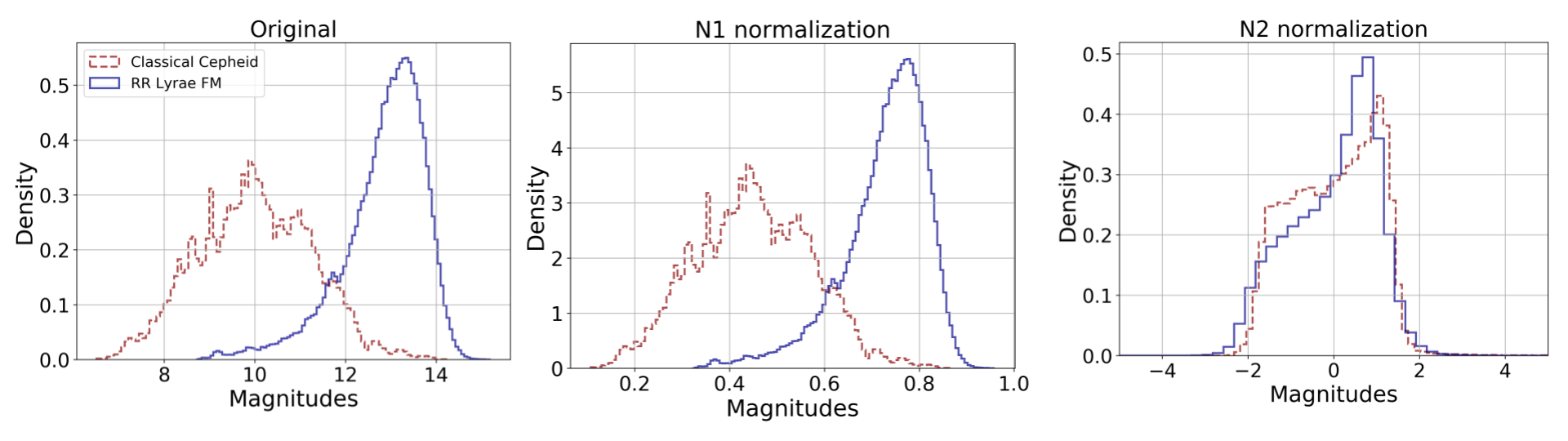
Figure 3: Cepheids and RR Lyrae magnitude distributions using different normalization methods. N1 normalizes using the minimum and maximum values across all lightcurves. N2 normalizes each sample separately, so they get zero mean and unit standard deviation.

4.1.2 Padding Lightcurves

Working with real lightcurves implies dealing with the variable-length problem of time series. The number of observations between astronomical objects differs and, therefore, it is not possible to train a matrix-based model such as neural networks. Consequently, we need to standardize the length among samples.

The most typical solutions rely on the interpolation and padding of lightcurves. Interpolation consists of estimating intermediate values in the observation sequence. On the other hand, the padding technique equalizes the lengths by inserting filler values (typically zero) and removing them during loss calculation. This technique is also known as zero-padding. In this work, we use the padding technique since interpolation could affect the underlying astrophysics properties of the lightcurves.

Even though zero padding solved the variable-length problem, a large variance in the number of observations could be inefficient in memory management. For example, on the ASAS dataset, the longest lightcurve has 1745 observations, while the shortest has 7 observations (see Table 3). Using the padding technique implies masking 1738 dummy observations for the shortest lightcurve or, in other words, 1738 loop-operations without contribution to training.

We sampled from the original lightcurves to reduce the variance in the number of observations, as shown in Figure 4. Each dashed line on the top chart defines a subset. The input of the network will be $L^{\prime}$ consecutive time steps such that $L^{\prime}<L$ the original number of observations. In this work, we defined $L^{\prime}=200$. It is important to highlight we only sample during training, so we use the full length lightcurves on testing. The subsampling process is also an alternative to the truncated backpropagation (Werbos et al., 1990), which decomposes the gradient as a sum of the losses at each time step (Puskorius & Feldkamp, 1994).

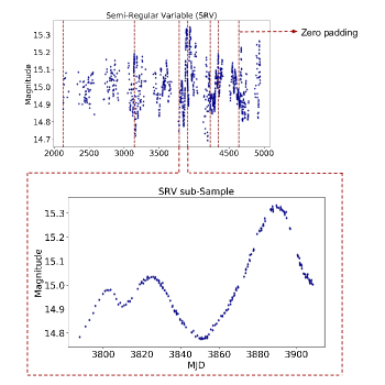
Figure 4: Masking and split preprocess step. A semi regular variable (SRV) from OGLE-III dataset is shown on the top chart. On the bottom figure, a zoom over a subsample of 200 observations is displayed in order to visualize the new input of the network. If we have less than 200 observations, we fill the last split with zeros (see the zero-padding portion in the top figure).

4.2 Neural Network Architecture

The network architecture is presented in Figure 5. We use two unidirectional layers of RNN, where $\sum$, the recurrent unit, is either LSTM or PLSTM. Both layers have the same number of neurons ($H=256$) and are initialized with zero states $(c_{0},h_{0})$. We use a batch size of B=400 samples for training. Notice that an epoch consists of $N/B$ iterations, where $N$ is the number of samples.

We apply layer normalization according to Ba et al. 2016 over each recurrent unit output. Additionally, we use a dropout (Semeniuta et al., 2016) of 0.5 probability over the second-layer output. The last part of the architecture is a Fully Connected ($FC$) classifier, which uses the hidden state to build a $K$-dim probability vector; $K$ is the number of classes.

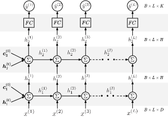
Figure 5: Recurrent network architecture. $B$, $L$, $H$, $D$ and $K$ are the batch size (or number of samples), time steps, hidden units, input parameters, and number of classes, respectively. The $\sum$ symbol represents the recurrent unit operations. The first layer receives the input matrix $x^{(l)}$ with $l=\{0,...,L\}$ and the states $c^{(l)}$, $h^{(l)}$. Note that the 0 superscript at the beginning defines the initial states while the recurrent layer is defined by the subscript. In the third layer we used a fully connected layer ($FC$) + softmax to obtain the class probabilities.

After training, we fix the best weight configuration for the LSTM and PLSTM classifiers, and we compute the forward pass to generate [$\boldsymbol{\hat{y}_{0}}$, $\boldsymbol{\hat{y}_{1}}$], the corresponding probability vectors, as shown in Figure 6. The final prediction $\boldsymbol{\hat{y}}$ is the average between the predictions. We named this testing setup the L+P architecture.

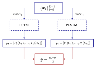
Figure 6: Testing architecture based on the combination of LSTM and PLSTM adjusted models.

4.3 Backpropagation

The backpropagation step (Boden, 2002), starts with the loss estimation that was carried out by the categorical cross-entropy (CCE) function (also called softmax loss). For each $b$-th batch sample, we calculate the corresponding loss at each $l$-th time step as follows:

$$\mathcal{L_{CCE}}(\hat{\rm{Y}}_{B\times L\times K})=-\frac{1}{B}\sum_{b=1}^{B}\sum_{l=1}^{L}\sum_{k=1}^{K}y_{bk}\log(\hat{y}_{blk}).$$ (16)

In the above formulation, $\boldsymbol{y}_{b}\in\mathbb{Z}^{K}$ is a one-hot vector associated with the class label of each $b$-th sample, and $\boldsymbol{\hat{y}}_{bl}\in\mathbb{R}^{K}$ is prediction vector at the $l$-th time step. Using the sum of losses along the $L$ time steps forces the network to predict as soon as possible, getting better classification results when we have fewer observations in the lightcurve.

Finally, we applied Adaptive Moment Estimation (ADAM) introduced by Kingma & Ba 2014 with an initial learning rate of 0.001 to update the network weights. The learning curves associated with the validation loss are presented in Appendix B.

4.4 Evaluation Metrics

Since the training sets are imbalanced, we employed the macro F1 score (Van Asch, 2013), a harmonic mean of precision and recall calculated separately for each $k\in K$ class,

$$\textrm{F1}=\frac{1}{K}\sum_{k=0}^{K-1}2\times\frac{\textrm{Precision}_{k}\times\textrm{Recall}_{k}}{\textrm{Precision}_{k}+\textrm{Recall}_{k}}$$

where,

$$\textrm{Recall}_{k}=\frac{\textrm{True Positives}_{k}}{\textrm{True Positives}_{k}+\textrm{False Negatives}_{k}}$$

$$\textrm{Precision}_{k}=\frac{\textrm{True Positives}_{k}}{\textrm{True Positives}_{k}+\textrm{False Positives}_{k}}.$$

The precision score determines how many of our predicted labels are actually true, and the recall indicates the number of true labels we were able to identify correctly. Using the macro average, all classes contribute equally regardless of how often they appear in the dataset.

4.5 Random Forest Classifier

As mentioned in previous sections, we used a Random Forest (RF) trained on features for comparison purposes. An RF is a classical machine learning method that combines the outputs of several decision trees for predicting (Breiman, 2001). Each decision tree splits the feature space to create isolated subgroups that separate objects with similar properties. We usually run a feature extraction process on the observations to characterize sequences using a standard set of descriptors. In this work, we use a python library published by (Nun et al., 2015) called FATS (Feature Analysis for Time Series), which facilitates the extraction of time-series features, such as the period and the autocorrelation function. Table 10 shows all the single-band features we selected for training. Because of library constraints, we only calculate features on lightcurves with at least ten observations.

4.6 Model Selection

We use k-fold cross-validation, with k=3. Each k-fold is composed of training (50%), validation (25%), and testing (25%) random subsets. We use the validation set during training to see how well our recurrent classifier generalizes over unseen objects. We perform the validation step at the end of each training epoch with a maximum of 2000 repetitions. However, we can stop the training process if the validation loss does not decrease compared to the best historical loss. In this case, we set 30 epochs as patience for the early stopping. In the case of RF, the validation set was used to find hyperparameters.

After $k$-fold training, we test our models using all available observations. For RNNs, we use the last hidden state of every lightcurve to build the final prediction. The best model is the one that maximizes the mean F1 scores of the cross-validated models.

5 Results

This section compares our model based on LSTM and PLSTM recurrent units with a RF trained on features and other models from the literature (Naul et al. 2018; Becker et al. 2020; Zorich et al. 2020).

Evaluation was shown to compute metrics using all available observations in the lightcurve (offline) and incrementally in-time (streaming). We observed significant improvements with the proposed recurrent model to classify lightcurves with less than 20 observations, being an excellent alternative to classify objects with less number of points in their lightcurves.

Next, we discuss the benefits of using recurrent models against an RF regarding the feature extraction process and time complexity. Confusion matrices and learning curves are shown in the Appendix A.

5.1 Offline Evaluation

We start by testing models using the whole lightcurve and evaluating them at the last time step. According to our cross-validation strategy (see Section 4.6), we ran each model 3 times. For each architecture, we select the type of normalization that maximizes the mean F1-score. Table 9 summarizes the performance of each model based on their precision, recall and F1-score.

For OGLE, WISE, Gaia, and LINEAR, the F1 score of the single LSTM and PLSTM are higher than that of RF. For MACHO, CSS, and ASAS, the PLSTM performs worse than the RF; however, the LSTM models outperform the RF. Combining PLSTM and LSTM recurrent neural networks works better in all datasets, obtaining the best performance in terms of the F1 score. Notice that for WISE, Gaia, LINEAR, and ASAS, the RF achieves a higher recall score than the neural-based models. However, the RNNs models obtain a higher precision than the RF (except for the PLSTM trained on CSS data). We analyze these results in detail in Appendix A.

We compared the performance of our models against other state-of-the-art deep learning classifiers. Becker et al. 2020 applied a Gated Recurrent Unit (GRU Cho et al. 2014) over the unfolded lightcurves of WISE, OGLE, and Gaia. As shown in Table 9, our combination of LSTM and PLSTM models obtain a higher F1-score, outperforming Becker’s results.

For the LINEAR and ASAS datasets, we compare our model against the recurrent autoencoder trained over folded lightcurves by Naul et al. 2018. For the best configuration according to Table 9, we obtained an accuracy of 0.903 $\pm$ 0.007 for LINEAR and 0.971 $\pm$ 0.002 for ASAS. Naul et al. 2018 obtained an accuracy of 0.988 $\pm$ 0.003 for LINEAR, and 0.971 $\pm$ 0.006 for ASAS using folded lightcurves. However, our approach does not depend on folding the lightcurves, saving the computation time of calculating the periods. Naul et al. 2018 also report their accuracy over unfolded lightcurves, decreasing to 0.781 for LINEAR, significantly lower than our results. They did not explicitly report their accuracy for ASAS.

For the MACHO dataset, Zorich et al. 2020 reached an F1 score of 0.86 by using a RF with incremental features over two bands. They also obtain an F1 score of 0.91 using an RF trained on FATS features (Nun et al., 2015). Our model outperforms both results by obtaining an F1 score of 0.921 $\pm$ 0.017 even though we use only the B band.

Dataset	Model	Normalization	F1 Score	Recall	Precision
	LSTM	N1	0.881 $\pm$ 0.008	0.879 $\pm$ 0.006	0.878 $\pm$ 0.003
	PLSTM	N2	0.765 $\pm$ 0.034	0.803 $\pm$ 0.010	0.777 $\pm$ 0.023
	LSTM + PLSTM	N1 & N2	0.881 $\pm$ 0.005	0.881 $\pm$ 0.004	0.879 $\pm$ 0.005
	RF	N1	0.799 $\pm$ 0.025	0.842 $\pm$ 0.030	0.780 $\pm$ 0.017
OGLE	Becker et.al., 2020		0.737 $\pm$ 0.005	0.730 $\pm$ 0.005	0.777 $\pm$ 0.006
	LSTM	N1	0.598 $\pm$ 0.009	0.531 $\pm$ 0.008	0.543 $\pm$ 0.004
	PLSTM	N1	0.585 $\pm$ 0.006	0.529 $\pm$ 0.006	0.541 $\pm$ 0.006
	LSTM + PLSTM	N1 & N1	0.646 $\pm$ 0.034	0.537 $\pm$ 0.003	0.551 $\pm$ 0.002
	RF	N1	0.472 $\pm$ 0.006	0.563 $\pm$ 0.006	0.463 $\pm$ 0.007
WISE	Becker et.al., 2020		0.462 $\pm$ 0.004	0.450 $\pm$ 0.010	0.551 $\pm$ 0.055
	LSTM	N1	0.805 $\pm$ 0.016	0.734 $\pm$ 0.022	0.760 $\pm$ 0.016
	PLSTM	N1	0.802 $\pm$ 0.027	0.733 $\pm$ 0.006	0.754 $\pm$ 0.003
	LSTM + PLSTM	N1 & N1	0.863 $\pm$ 0.040	0.741 $\pm$ 0.009	0.772 $\pm$ 0.010
	RF	N1	0.591 $\pm$ 0.000	0.814 $\pm$ 0.004	0.569 $\pm$ 0.000
GAIA	Becker et.al., 2020		0.668 $\pm$ 0.004	0.657 $\pm$ 0.006	0.713 $\pm$ 0.007
	LSTM	N2	0.858 $\pm$ 0.016	0.848 $\pm$ 0.019	0.851 $\pm$ 0.003
	PLSTM	N2	0.764 $\pm$ 0.026	0.763 $\pm$ 0.042	0.758 $\pm$ 0.030
	LSTM + PLSTM	N2 & N1	0.877 $\pm$ 0.021	0.822 $\pm$ 0.023	0.844 $\pm$ 0.008
LINEAR	RF	N1	0.736 $\pm$ 0.007	0.850 $\pm$ 0.012	0.687 $\pm$ 0.008
	LSTM	N2	0.836 $\pm$ 0.037	0.814 $\pm$ 0.012	0.813 $\pm$ 0.019
	PLSTM	N2	0.755 $\pm$ 0.032	0.771 $\pm$ 0.014	0.745 $\pm$ 0.018
	LSTM + PLSTM	N2 & N1	0.921 $\pm$ 0.017	0.867 $\pm$ 0.008	0.886 $\pm$ 0.015
MACHO	RF	N1	0.787 $\pm$ 0.082	0.818 $\pm$ 0.087	0.772 $\pm$ 0.078
	LSTM	N2	0.500 $\pm$ 0.027	0.506 $\pm$ 0.011	0.490 $\pm$ 0.016
	PLSTM	N1	0.396 $\pm$ 0.008	0.403 $\pm$ 0.016	0.386 $\pm$ 0.013
	LSTM + PLSTM	N2 & N1	0.505 $\pm$ 0.030	0.519 $\pm$ 0.019	0.496 $\pm$ 0.020
CSS	RF	N1	0.464 $\pm$ 0.004	0.493 $\pm$ 0.004	0.474 $\pm$ 0.006
	LSTM	N2	0.931 $\pm$ 0.005	0.902 $\pm$ 0.027	0.911 $\pm$ 0.017
	PLSTM	N2	0.892 $\pm$ 0.020	0.894 $\pm$ 0.016	0.891 $\pm$ 0.014
	LSTM + PLSTM	N2 & N1	0.957 $\pm$ 0.007	0.920 $\pm$ 0.015	0.935 $\pm$ 0.011
ASAS	RF	N1	0.917 $\pm$ 0.023	0.961 $\pm$ 0.012	0.891 $\pm$ 0.027

Table 9: Offline table corresponding to the model evaluation using the entire lightcurve. The first and second columns are associated with the dataset and the classification model, respectively. The third column denotes the normalization technique associated with the best cross-validated metrics on columns 4, 5, and 6. We also include the available scores from Becker et al. 2020, which is the current state of the art for WISE, Gaia, and OGLE.

Taking advantage of the PLSTM properties, we have shown that the L+P model improves the offline classification of lightcurves even when the single PLSTM performs worse than the other models (i.e., LSTM and RF). Our model is able to classify using unfolded lightcurves, which avoids the computational cost of calculating the period to fold the lightcurves, and the number of points needed to perform classification on a given lightcurve.

5.2 Streaming Evaluation

In Section 5.1, we evaluate our models using all lightcurve observations. However, when analyzing real-world data, we require classifying sources online (Borne 2007; Saha et al. 2014; Borne 2009; Förster et al. 2020). To assess our models’ quality in this scenario, we evaluate them in terms of the number of observations presented in the lightcurve.

Figure 9 shows the F1-score of the RF, LSTM, PLSTM, and L+P models for each dataset in terms of the number of points used for the classification. As we mention on Section 4, the classifiers were trained using all observations in the lightcurves subsamples, while this evaluation is performed in terms of the number of points of the lightcurves. As the number of observations increases, the F1 scores of neural-based models increase faster than those for the RF. We hypothesize that some pre-calculated features could be more affected by short-length lightcurves than the representations made by RNNs. We study this premise in Fig. 7, where we show the features importance according to the RF model for the LINEAR dataset. Attributes related to position, dispersion, and central tendency are important to separate classes in this case. These features depend on the number of observations. Conversely, RNNs propagate the classification error at each time step during training, forcing the network to discover better separability of the classes in early epochs.

Our L+P model takes advantage of the LSTM and PLSTM units, improving the scores at different instants of the lightcurve. In most cases, the LSTM and PLSTM models achieve similar results (with the exception of LINEAR and CSS, where the LSTM model significantly outperforms the PLSTM model). The L+P improves or equals the F1-score of the best models by averaging the probabilities of both recurrent architectures.

For the RF, most of the features need to be re-calculated when a new sample arrives, which is time-consuming compared to the RNNs. Figure 8 shows the mean and standard deviation of the prediction times for the feature-based classifier and RNNs tested on the entire sequence across all datasets. The execution time of the RFs for classifying lightcurves grows faster than RNNs because it depends on the feature extraction process. For example, the period estimation is $O(L\log L)$ and the autocorrelation function is $\mathcal{O}(L^{2})$, where $L$ is the number of observations. In contrast, RNNs only need to update the last hidden state, $\mathcal{O}(1)$ for a single observation and $\mathcal{O}(L)$ for the entire sequence.

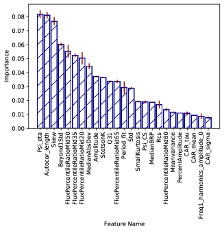
Figure 7: LINEAR Feature importance according to the Gini-score of the Random Forest classifier.

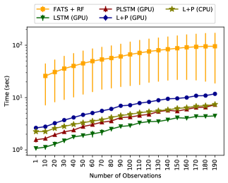
Figure 8: Testing run-times in function of the number of observations among different surveys.

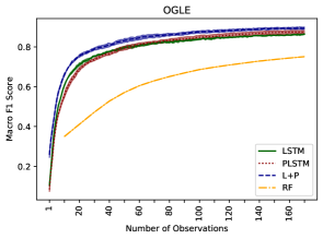
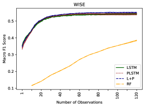
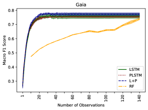
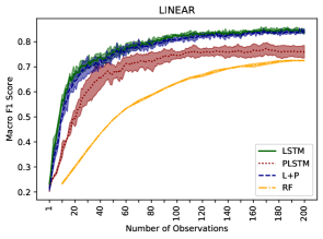
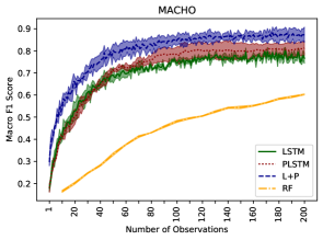
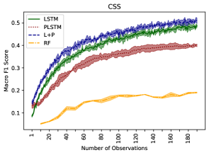
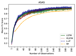
Figure 9: Streaming evaluation of the Random Forest (RF), Long Short Term Memory (LSTM), Phased LSTM (PLSTM), and the combination of both recurrent units (L+P) for each dataset. All curves show the mean and standard deviation of the macro F1 score as a function of the number of observations.

6 Conclusions

In this work, we addressed the problem of the automatic classification of unfolded real lightcurves. We introduced a deep learning model (L+P) that combines the output probabilities from an LSTM and PLSTM classifiers. Empirical evaluations on seven single-band catalogs, including periodic and nonperiodic astronomical objects, demonstrated the L+P model outperforms models trained on features and state-of-the-art classifiers.

We tested our proposed model both using the whole lightcurve and incrementally in time. The L+P architecture obtained the best F1 score among all datasets in both scenarios. Moreover, the model turned out to be an excellent alternative to classify short-length lightcurves where the number of observations is less than 20. The cumulative loss used to update weights forces the network to accurately predict all time steps, not just in the last observation.

Recurrent neural networks need only the last hidden state to predict new observations. The hidden states save features of the lightcurve up to the last observed point. The update process is O(1), which is ideal for streaming scenarios, unlike the RF that needs to recalculate features using all time steps.

Since the neural-based models learn representations of the unprocessed raw data, we can capture features without restricting the domain using prior knowledge, such as the object’s periodicity. However, the optimization process may be suboptimal when we have a low number of samples to fit the model parameters. Future works will focus on providing more information to the network by adding, for example, stellar coordinates or multiple bands during training.

We have proved the robustness of our architecture on different kinds of stars and astronomical catalogs. Our classifier works on unfolded periodic and nonperiodic lightcurves, achieving comparable or better-than results than other state-of-the-art approaches. We will continue to delve into these neural architectures facing the new generation of telescopes and their new real-world applications.

Data Availability

All data can be found at https://drive.google.com/drive/folders/1m2fXqn25LYSyG5jEbpM3Yfdbpx9EQCDo?usp=sharing or downloading directly as indicated in https://github.com/cridonoso/plstm_tf2.

Appendix A Confusion Matrices

This section presents and analyzes the confusion matrices associated with the best L+P and RF results, according to Table 9. Figures 10-16 show the confusion matrices for the seven datasets we used in this work. Each percentage within the matrices indicates the classifier prediction as a fraction of the total number of true labels per class. Note that low dispersion in rows is related to a high precision score. Similarly, a high recall score is associated with low dispersion in columns.

Confusion matrices show that the L+P model tends to be more precise than RF when predicting. RNNs learn representations of data to separate classes while the RF receives predefined features, standard for any time series. However, recurrent models depend strongly on the training set, which directly affects the representation’s quality. For example, in Figure 12, the L+P can identify most of the ab-type RR Lyrae ($RRab$), but it is missing all c-type RRLyra ($RRc$), and most of the SX Phoenicis Delta Scuti (DSCT_SXPHE).

High precision scores often expose an overfitting problem related to class imbalance. In the example of Figure 12, the $RRab$ has 16412 samples versus the 3831 $RRc$ and 1098 DSCT_SXPHE. It means that $RRab$ dominates training in terms of the number of samples, that the learned features will therefore be loaded towards this class. Though the network overfits $RRab$, it can separate similar pulsating time-scales, such as $\delta$-scutis and RR Lyrae, because of their variability similitude. We use red boxes inside the matrices for grouping similar classes. We hypothesize that the significant variance in time scales (see Table 8) affects the network to separate short-period objects.

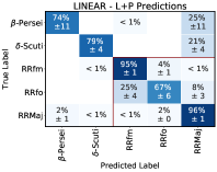
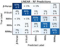
Figure 10: LINEAR confusion matrices for the predictions of the LSTM+PLSTM (L+P) and the Random Forest (RF) classifiers.

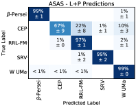
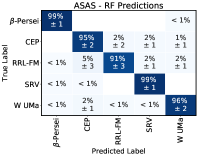
Figure 11: ASAS confusion matrices for the predictions of the LSTM+PLSTM (L+P) and the Random Forest (RF) classifiers.

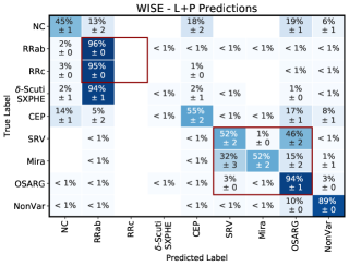
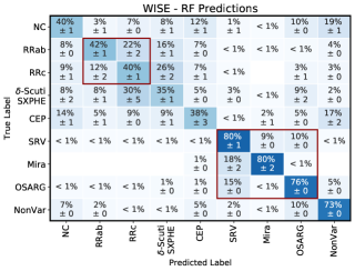
Figure 12: WISE confusion matrices for the predictions of the LSTM+PLSTM (L+P) and the Random Forest (RF) classifiers.

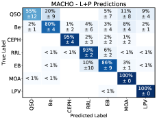
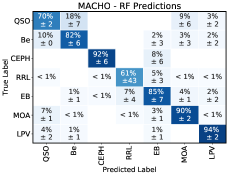
Figure 13: MACHO confusion matrices for the predictions of the LSTM+PLSTM (L+P) and the Random Forest (RF) classifiers.

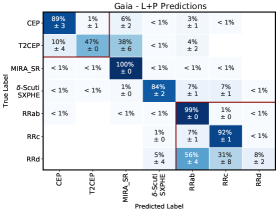
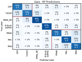
Figure 14: Gaia confusion matrices for the predictions of the LSTM+PLSTM (L+P) and the Random Forest (RF) classifiers.

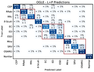
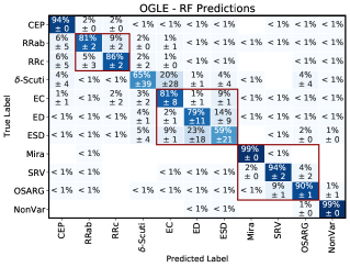
Figure 15: OGLE confusion matrices for the predictions of the LSTM+PLSTM (L+P) and the Random Forest (RF) classifiers.

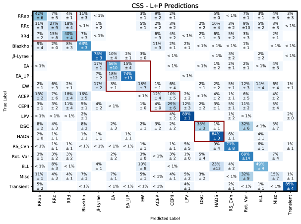
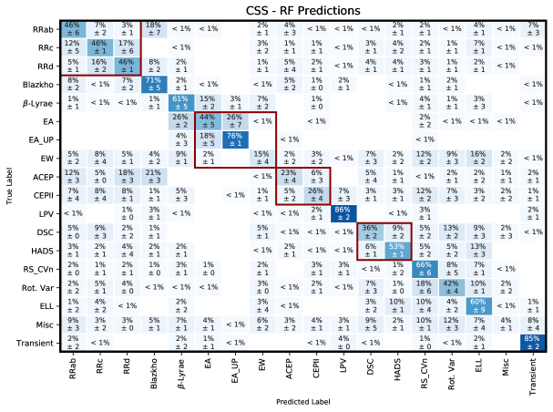
Figure 16: CSS confusion matrices for the predictions of the LSTM+PLSTM (L+P) and the Random Forest (RF) classifiers.

Appendix B Learning Curves

Figure 17 shows the learning curves corresponding to the LSTM and PLSTM, trained with min-max scaler (N1) and standardization (N2) as input normalization technique. Each plot presents the mean and standard deviation of the validation losses according to the cross-validation strategy explained in section 4.6.

In all datasets, the N2 normalization converged faster than the N1. However, it is not a guarantee of achieving the best validation loss. For example, in the WISE and Gaia dataset, the model trained on lightcurves N2 converged faster than N1 but with a worse validation loss.

In general, the N2 normalization is similar to N1 in terms of minimum values but slower to converge. However, since the N2 normalization shift and scales lightcurves to have zero mean and unit standard deviation, the optimization becomes more manageable than in N1. We can see this effect in the variance of the learning curves in Figure B. We also tried using N1 on each lightcurve separately and N2 over the entire dataset. However, the results were not significant, and we empirically decided to use the highest scoring alternatives.

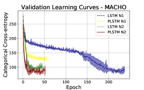
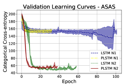
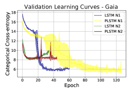
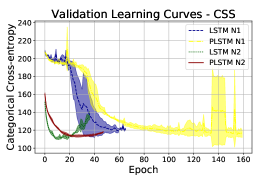
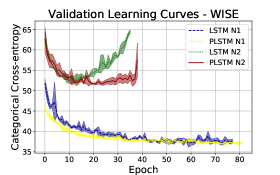
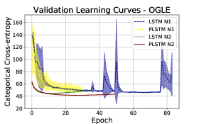
Figure 17: Validation Loss for the LSTM and PLSTM. The curves show the mean and standard deviation of the 3-fold execution. The input was normalized using min-max scaler (N1) or z-score standardization (N2)

Appendix C FATS features

Table 10 shows the features used to train the RF model. We used all single-band features on lightcurves with at least 10 observations.

FATS Feature Name	Reference
MedianAbsDev	Richards et al. (2011)
PeriodLS	Kim et al. (2011)
Autocor_length	Kim et al. (2011)
Q31	Kim et al. (2014)
FluxPercentileRatioMid35	Richards et al. (2011)
FluxPercentileRatioMid50	Richards et al. (2011)
FluxPercentileRatioMid65	Richards et al. (2011)
FluxPercentileRatioMid20	Richards et al. (2011)
Beyond1Std	Richards et al. (2011)
Skew	Richards et al. (2011)
Con	Kim et al. (2014)
Gskew	Nun et al. (2015)
Meanvariance	Kim et al. (2011)
StetsonK	Richards et al. (2011)
FluxPercentileRatioMid80	Richards et al. (2011)
CAR_sigma	Pichara et al. (2012)
CAR_mean	Pichara et al. (2012)
CAR_tau	Pichara et al. (2012)
MedianBRP	Richards et al. (2011)
Rcs	Kim et al. (2011)
Std	Richards et al. (2011)
SmallKurtosis	Richards et al. (2011)
Mean	Kim et al. (2014)
Amplitude	Richards et al. (2011)
StructureFunction_index_21	Nun et al. (2015)
StructureFunction_index_31	Nun et al. (2015)
Freq1_harmonics_amplitude_0	Richards et al. (2011)

Table 10: FATS features used for Random Forest training

FATS Feature Name	Reference
Freq1_harmonics_amplitude_1	Richards et al. (2011)
Freq1_harmonics_amplitude_2	Richards et al. (2011)
Freq1_harmonics_amplitude_3	Richards et al. (2011)
Freq1_harmonics_rel_phase_0	Richards et al. (2011)
Freq1_harmonics_rel_phase_1	Richards et al. (2011)
Freq1_harmonics_rel_phase_2	Richards et al. (2011)
Freq1_harmonics_rel_phase_3	Richards et al. (2011)
Freq2_harmonics_amplitude_0	Richards et al. (2011)
Freq2_harmonics_amplitude_1	Richards et al. (2011)
Freq2_harmonics_amplitude_2	Richards et al. (2011)
Freq2_harmonics_amplitude_3	Richards et al. (2011)
Freq2_harmonics_rel_phase_0	Richards et al. (2011)
Freq2_harmonics_rel_phase_1	Richards et al. (2011)
Freq2_harmonics_rel_phase_2	Richards et al. (2011)
Freq2_harmonics_rel_phase_3	Richards et al. (2011)
Freq3_harmonics_amplitude_0	Richards et al. (2011)
Freq3_harmonics_amplitude_1	Richards et al. (2011)
Freq3_harmonics_amplitude_2	Richards et al. (2011)
Freq3_harmonics_amplitude_3	Richards et al. (2011)
Freq3_harmonics_rel_phase_0	Richards et al. (2011)
Freq3_harmonics_rel_phase_1	Richards et al. (2011)
Freq3_harmonics_rel_phase_2	Richards et al. (2011)
Freq3_harmonics_rel_phase_3	Richards et al. (2011)
Psi_CS	Kim et al. (2014)
Psi_eta	Kim et al. (2014)
AndersonDarling	Kim et al. (2009)
LinearTrend	Richards et al. (2011)
PercentAmplitude	Richards et al. (2011)
MaxSlope	Richards et al. (2011)
PairSlopeTrend	Richards et al. (2011)
Period_fit	Kim et al. (2011)
StructureFunction_index_32	Nun et al. (2015)

References

- Abbott et al. (2017a) Abbott B. P., et al., 2017a, Astrophys. J. Lett, 848, L12
- Abbott et al. (2017b) Abbott B. P., et al., 2017b, The Astrophysical Journal Letters, 848, L13
- Alcock et al. (1995) Alcock C., et al., 1995, arXiv preprint astro-ph/9506113
- Alcock et al. (2000) Alcock C., et al., 2000, The Astrophysical Journal, 542, 281
- Anumula et al. (2018) Anumula J., Neil D., Delbruck T., Liu S.-C., 2018, Frontiers in neuroscience, 12, 23
- Ba et al. (2016) Ba J. L., Kiros J. R., Hinton G. E., 2016, arXiv preprint arXiv:1607.06450
- Bai et al. (2018) Bai Y., Liu J.-F., Wang S., 2018, Research in Astronomy and Astrophysics, 18, 118
- Becker et al. (2020) Becker I., Pichara K., Catelan M., Protopapas P., Aguirre C., Nikzat F., 2020, Monthly Notices of the Royal Astronomical Society
- Bellm et al. (2018) Bellm E. C., et al., 2018, Publications of the Astronomical Society of the Pacific, 131, 018002
- Boden (2002) Boden M., 2002, the Dallas project
- Bonanos (2006) Bonanos A. Z., 2006, Proceedings of the International Astronomical Union, 2, 79
- Boone (2019) Boone K., 2019, The Astronomical Journal, 158, 257
- Borne (2007) Borne K. D., 2007, Next generation of data mining and cyber-enabled discovery for innovation (NGDM07)
- Borne (2009) Borne K., 2009, arXiv preprint arXiv:0911.0505
- Breiman (2001) Breiman L., 2001, Machine learning, 45, 5
- Cabrera-Vives et al. (2017) Cabrera-Vives G., Reyes I., Förster F., Estévez P. A., Maureira J.-C., 2017, The Astrophysical Journal, 836, 97
- Carrasco-Davis et al. (2019) Carrasco-Davis R., et al., 2019, Publications of the Astronomical Society of the Pacific, 131, 108006
- Castro et al. (2017) Castro N., Protopapas P., Pichara K., 2017, The Astronomical Journal, 155, 16
- Castro et al. (2018) Castro N., Protopapas P., Pichara K., 2018, arXiv preprint arXiv:1801.09732
- Chaini & Kumar (2020) Chaini S., Kumar S. S., 2020, arXiv preprint arXiv:2006.12333
- Charnock & Moss (2017) Charnock T., Moss A., 2017, The Astrophysical Journal Letters, 837, L28
- Cho et al. (2014) Cho K., Van Merriënboer B., Gulcehre C., Bahdanau D., Bougares F., Schwenk H., Bengio Y., 2014, arXiv preprint arXiv:1406.1078
- Collaboration et al. (2016) Collaboration G., et al., 2016, arXiv preprint arXiv:1609.04153
- Devine et al. (2018) Devine T. R., Goseva-Popstojanova K., Pang D., 2018, in Proceedings of the 47th International Conference on Parallel Processing. p. 11
- Dieleman et al. (2015) Dieleman S., Willett K. W., Dambre J., 2015, Monthly notices of the royal astronomical society, 450, 1441
- Drake et al. (2009) Drake A., et al., 2009, The Astrophysical Journal, 696, 870
- Förster et al. (2020) Förster F., et al., 2020, arXiv preprint arXiv:2008.03303
- Fotopoulou & Paltani (2018) Fotopoulou S., Paltani S., 2018, Astronomy & Astrophysics, 619, A14
- Gaia et al. (2018) Gaia C., et al., 2018, Astronomy & Astrophysics, 616
- George & Huerta (2018) George D., Huerta E., 2018, Physical Review D, 97, 044039
- Glorot & Bengio (2010) Glorot X., Bengio Y., 2010, in Proceedings of the thirteenth international conference on artificial intelligence and statistics. pp 249–256
- Gómez et al. (2020) Gómez C., Neira M., Hoyos M. H., Arbeláez P., Forero-Romero J. E., 2020, arXiv preprint arXiv:2004.13877
- Gravet et al. (2015) Gravet R., et al., 2015, The Astrophysical Journal Supplement Series, 221, 8
- Greff et al. (2016) Greff K., Srivastava R. K., Koutník J., Steunebrink B. R., Schmidhuber J., 2016, IEEE transactions on neural networks and learning systems, 28, 2222
- He et al. (2015) He K., Zhang X., Ren S., Sun J., 2015, in Proceedings of the IEEE international conference on computer vision. pp 1026–1034
- Hochreiter & Schmidhuber (1997a) Hochreiter S., Schmidhuber J., 1997a, in Advances in neural information processing systems. pp 473–479
- Hochreiter & Schmidhuber (1997b) Hochreiter S., Schmidhuber J., 1997b, Neural computation, 9, 1735
- Ivezić et al. (2019) Ivezić Ž., et al., 2019, The Astrophysical Journal, 873, 111
- Jamal & Bloom (2020) Jamal S., Bloom J. S., 2020, arXiv preprint arXiv:2003.08618
- Jayalakshmi & Santhakumaran (2011) Jayalakshmi T., Santhakumaran A., 2011, International Journal of Computer Theory and Engineering, 3, 1793
- Kim et al. (2009) Kim D.-W., Protopapas P., Alcock C., Byun Y.-I., Bianco F. B., 2009, Monthly Notices of the Royal Astronomical Society, 397, 558
- Kim et al. (2011) Kim D.-W., Protopapas P., Byun Y.-I., Alcock C., Khardon R., Trichas M., 2011, The Astrophysical Journal, 735, 68
- Kim et al. (2014) Kim D.-W., Protopapas P., Bailer-Jones C. A., Byun Y.-I., Chang S.-W., Marquette J.-B., Shin M.-S., 2014, Astronomy & Astrophysics, 566, A43
- Kingma & Ba (2014) Kingma D. P., Ba J., 2014, arXiv preprint arXiv:1412.6980
- LeCun et al. (2015) LeCun Y., Bengio Y., Hinton G., 2015, nature, 521, 436
- Liu et al. (2018) Liu L., Shen J., Zhang M., Wang Z., Tang J., 2018, in Thirty-Second AAAI Conference on Artificial Intelligence.
- Lochner et al. (2016) Lochner M., McEwen J. D., Peiris H. V., Lahav O., Winter M. K., 2016, The Astrophysical Journal Supplement Series, 225, 31
- Mackenzie et al. (2016) Mackenzie C., Pichara K., Protopapas P., 2016, The Astrophysical Journal, 820, 138
- Mahabal et al. (2017) Mahabal A., Sheth K., Gieseke F., Pai A., Djorgovski S. G., Drake A. J., Graham M. J., 2017, in 2017 IEEE Symposium Series on Computational Intelligence (SSCI). pp 1–8
- Mahabal et al. (2019) Mahabal A., et al., 2019, Publications of the Astronomical Society of the Pacific, 131, 038002
- Martínez-Palomera et al. (2018) Martínez-Palomera J., et al., 2018, The Astronomical Journal, 156, 186
- Möller & de Boissière (2020) Möller A., de Boissière T., 2020, Monthly Notices of the Royal Astronomical Society, 491, 4277
- Mondrik et al. (2015) Mondrik N., Long J., Marshall J., 2015, The Astrophysical Journal Letters, 811, L34
- Moss (2018) Moss A., 2018, arXiv preprint arXiv:1810.06441
- Muthukrishna et al. (2019) Muthukrishna D., Narayan G., Mandel K. S., Biswas R., Hložek R., 2019, arXiv preprint arXiv:1904.00014
- Naul et al. (2018) Naul B., Bloom J. S., Pérez F., van der Walt S., 2018, Nature Astronomy, 2, 151
- Neil et al. (2016) Neil D., Pfeiffer M., Liu S.-C., 2016, in Advances in Neural Information Processing Systems. pp 3882–3890
- Neira et al. (2020) Neira M., Gómez C., Suárez-Pérez J. F., Gómez D. A., Reyes J. P., Hoyos M. H., Arbeláez P., Forero-Romero J. E., 2020, The Astrophysical Journal Supplement Series, 250, 11
- Nikutta et al. (2014) Nikutta R., Hunt-Walker N., Nenkova M., Ivezić Ž., Elitzur M., 2014, Monthly Notices of the Royal Astronomical Society, 442, 3361
- Nun et al. (2014) Nun I., Pichara K., Protopapas P., Kim D.-W., 2014, The Astrophysical Journal, 793, 23
- Nun et al. (2015) Nun I., Protopapas P., Sim B., Zhu M., Dave R., Castro N., Pichara K., 2015, arXiv preprint arXiv:1506.00010
- Oh & Jung (2004) Oh K.-S., Jung K., 2004, Pattern Recognition, 37, 1311
- Palaversa et al. (2013) Palaversa L., et al., 2013, The Astronomical Journal, 146, 101
- Pascanu et al. (2012) Pascanu R., Mikolov T., Bengio Y., 2012, CoRR, abs/1211.5063, 2
- Pichara et al. (2012) Pichara K., Protopapas P., Kim D.-W., Marquette J.-B., Tisserand P., 2012, Monthly Notices of the Royal Astronomical Society, 427, 1284
- Pietrzyński (2018) Pietrzyński G., 2018, Twenty-five years of using microlensing to study dark matter
- Pojmanski & Maciejewski (2005) Pojmanski G., Maciejewski G., 2005, Acta Astronomica, 55, 97
- Puskorius & Feldkamp (1994) Puskorius G., Feldkamp L., 1994, in Neural Networks, 1994. IEEE World Congress on Computational Intelligence., 1994 IEEE International Conference on. pp 2488–2493
- Richards et al. (2011) Richards J. W., et al., 2011, The Astrophysical Journal, 733, 10
- Rumelhart et al. (1986) Rumelhart D. E., Hinton G. E., Williams R. J., 1986, nature, 323, 533
- Saha et al. (2014) Saha A., Matheson T., Snodgrass R., Kececioglu J., Narayan G., Seaman R., Jenness T., Axelrod T., 2014, in Observatory Operations: Strategies, Processes, and Systems V. p. 914908
- Sánchez-Sáez et al. (2021) Sánchez-Sáez P., et al., 2021, The Astronomical Journal, 161, 141
- Sánchez et al. (2019) Sánchez B., et al., 2019, Astronomy and Computing, 28, 100284
- Schulze et al. (2018) Schulze S., et al., 2018, Monthly Notices of the Royal Astronomical Society, 473, 1258
- Semeniuta et al. (2016) Semeniuta S., Severyn A., Barth E., 2016, arXiv preprint arXiv:1603.05118
- Shanker et al. (1996) Shanker M., Hu M. Y., Hung M. S., 1996, Omega, 24, 385
- Stokes et al. (2000) Stokes G. H., Evans J. B., Viggh H. E., Shelly F. C., Pearce E. C., 2000, Icarus, 148, 21
- Tammann et al. (2008) Tammann G. A., Sandage A., Reindl B., 2008, The Astronomy and Astrophysics Review, 15, 289
- Udalski (2004) Udalski A., 2004, arXiv preprint astro-ph/0401123
- Udalski et al. (1997) Udalski A., Kubiak M., Szymanski M., 1997, arXiv preprint astro-ph/9710091
- Valenzuela & Pichara (2018) Valenzuela L., Pichara K., 2018, Monthly Notices of the Royal Astronomical Society, 474, 3259
- Van Asch (2013) Van Asch V., 2013, Belgium: CLiPS, 49
- VanderPlas (2018) VanderPlas J. T., 2018, The Astrophysical Journal Supplement Series, 236, 16
- Villar et al. (2019) Villar V., et al., 2019, arXiv preprint arXiv:1905.07422
- Werbos et al. (1990) Werbos P. J., et al., 1990, Proceedings of the IEEE, 78, 1550
- Wright et al. (2010) Wright E. L., et al., 2010, AJ, 140, 1868
- Zorich et al. (2020) Zorich L., Pichara K., Protopapas P., 2020, Monthly Notices of the Royal Astronomical Society, 492, 2897