Light dark matter, rare $B$ decays with missing energy in $L_{\mu}-L_{\tau}$ model with a scalar leptoquark

Abstract

We investigate the phenomenology of light GeV-scale fermionic dark matter in $U(1)_{L_{\mu}-L_{\tau}}$ gauge extension of the Standard Model. Heavy neutral fermions alongside with a $S_{1}(\overline{3}$,$1$,$1/3$) scalar leptoquark and an inert scalar doublet are added to address the flavor anomalies and light neutrino mass respectively. The light gauge boson associated with $U(1)_{L_{\mu}-L_{\tau}}$ gauge group mediates dark to visible sector and helps to obtain the correct relic density. Aided with a colored scalar, we constrain the new model parameters by using the branching ratios of various $b\to sll$ and $b\to s\gamma$ decay processes as well as the lepton flavour non-universality observables $R_{K^{(*)}}$ and then show the implication on the branching ratios of some rare semileptonic $B\to(K^{(*)},\phi)+$ missing energy, processes.

I Introduction

Standard Model (SM) of particle physics is quite successful in meeting the experimental sensitivities when it comes to interactions at fundamental level. It is believed to be a low-energy gauge theory embedded in a high scale unified version. Despite its accomplishments, the increasing sensitivities of various intensity and cosmic frontier experiments have spotlighted its drawbacks and hints towards its extension. Listing a few, the existence of dark matter (DM) and its nature Zwicky (1937); Rubin and Ford (1970); Clowe et al. (2004); Bertone et al. (2005); Arkani-Hamed et al. (2009); Dodelson and Widrow (1994), non-zero neutrino masses and its mixing phenomena Zyla et al. (2020), matter-antimatter asymmetry Sakharov (1991); Kolb and Wolfram (1980); Davidson et al. (2008); Buchmuller et al. (2005); Strumia (2006) etc.

Though most of the flavor observables go along with the SM, there are a collection of recent measurements in semileptonic $B$ meson decays, involving $b\to sll$ and $b\to c\tau\bar{\nu}_{\tau}$ quark level transitions, that are incongruous with the SM predictions. The most conspicuous measurements, hinting the physics beyond SM are the lepton flavor universality violating parametes: $R_{K}$ with a discrepancy of $3.1\sigma$ Aaij et al. (2014a, 2019, 2021); Bobeth et al. (2007); Bordone et al. (2016), $R_{K^{(*)}}$ with a disagreement at the level of $(2.1-2.5)\sigma$ Aaij et al. (2017); Capdevila et al. (2018), $R_{D^{(*)}}$ with $3.08\sigma$ discrepancy Amhis et al. (2019); Na et al. (2015); Fajfer et al. (2012a, b) and $R_{J/\psi}$ with a deviation of nearly $2\sigma$ Aaij et al. (2018); Wang et al. (2013); Ivanov et al. (2005) from their SM predictions. Though the Belle Collaboration Abdesselam et al. (2019a, b) has also announced their measurements on $R_{K^{(*)}}$ in various $q^{2}$ bins, however these measurements have large uncertainties. Besides the $R_{K^{(*)}}$ parameters, the $P_{5}^{\prime}$ optimized observable disagrees with the SM at the level of $4\sigma$ in the $(4.3-8.68)~{}\rm{GeV}^{2}$ $q^{2}$-bin Aaij et al. (2013a, 2016); Abdesselam et al. (2016) and the decay rate of $B\to K^{*}\mu\mu$ shows $3\sigma$ discrepancy Aaij et al. (2014b). The branching ratio of $B_{s}\to\phi\mu\mu$ channel also disagrees with the theory at the level of $3\sigma$ Aaij et al. (2013b) in low $q^{2}$.

Due to the above discussed anomalies in $b\to sll$, the rare semileptonic $B$ decays with charged leptons in the final state such as $B\to K^{(*)}ll$, $B_{s}\to\phi ll$ have attracted large attention in recent times compared to the analogous semileptonic $B$ meson channels with neutral leptons in the final state, i.e., $B\to K^{(*)}\nu\bar{\nu}$, $B_{s}\to\phi\nu\bar{\nu}$. Since the neutrinos escape undetected, the number of angular observables associated with charged leptons are also more in contrast to the $b\to s\nu\bar{\nu}$ processes. In the SM, the rare $b\to s\nu\bar{\nu}$ transitions are significantly suppressed by the loop momentum and off-diagonal CKM matrix elements. Even though these processes are theoretically very clean compared to other FCNC decays, these are yet to be observed; there exist only upper limits in the branching ratios of such decays Zyla et al. (2020). The theoretical computation of inclusive $B\to X_{s}\nu\bar{\nu}$ process is quite easy, however the experimental measurement of this decay is probably unfeasible due to the requirement of reconstruction of all $X_{s}$ and the missing neutrinos. However, the exclusive $B\to K^{(*)}\nu\bar{\nu}$ processes are more promising to look for physics beyond the SM.

Of particular interest among the FCNC $B$ decays are the semileptonic decays of the form $b\to s+\displaystyle{\not}{E}$, where $\displaystyle{\not}E$ stands for the missing energy. Besides the production of heavy meson in charge and CP correlated states, the existing $B$-factories can tag the missing energy decays of $B$ meson “on the other side”. In Ref. Badin and Petrov (2010), the leptonic decays of heavy $B(D)$ meson to a pair of scalar or fermion or vector particles has been investigated both in model independent way and in some popular models. Many new physics models Aslam and Lu (2009); Aliev et al. (2007); Altmannshofer et al. (2009a); Kim and Wang (2008); Jeon et al. (2006); Kim and Wang (2009); Sirvanli (2008); Smith (2010); Mahajan (2003) also have been proposed to test the observed rates of $B\to M+\displaystyle{\not}E$ decays. Furthermore, the sensitivity of bounds on WIMP-nucleon cross section for GeV scale dark matter in direct detection experiments is less. This brings us to study a light GeV scale WIMP ($<2.5$ GeV) in the light of missing energy in rare $B$-decays.

To input our purpose, we opt for a simple but phenomenologically rich the $U(1)_{L_{\mu}-L_{\tau}}$ gauge extension. Proposed by X.G. He et al, in He et al. (1991a, b), and then later explored to explain muon $g-2$, dark matter, neutrino phenomenology and matter-antimatter asymmetry of the Universe Ma et al. (2002); Baek and Ko (2009); Altmannshofer et al. (2014a); Heeck et al. (2015); Crivellin et al. (2015); Fuyuto et al. (2016); Patra et al. (2016); Biswas et al. (2016); Altmannshofer et al. (2016); Araki et al. (2017); Chen and Nomura (2017, 2018); Baek (2018); Bauer et al. (2018); Kamada et al. (2018); Gninenko and Krasnikov (2018); Nomura and Okada (2018); Banerjee and Roy (2019); Heeck et al. (2019); Escudero et al. (2019); Altmannshofer et al. (2019); Biswas and Shaw (2019); Kowalska et al. (2019); Kang and Shigekami (2019); Joshipura et al. (2020); Han et al. (2019); Jho et al. (2020); Amaral et al. (2020); Borah et al. (2020); Huang et al. (2021); Borah et al. (2021). In our previous work Singirala et al. (2019), we extended this model with three heavy neutral fermions, a $(\overline{3},1,1/3)$ scalar leptoquark and investigated heavy fermion DM and various flavor anomalies. In the present work, we look at low mass regime of DM arising as a missing energy in semileptonic decays of $B$ meson to $M(=K,K^{*},\phi)$. The extant of LQ is proposed in many theoretical frameworks, such as the grand unified theories Georgi and Glashow (1974); Fritzsch and Minkowski (1975); Langacker (1981); Georgi (1975), Pati-Salam model Pati and Salam (1974, 1973a, 1973b); Shanker (1982a, b), quark and lepton composite model Kaplan (1991) and the technicolor model Schrempp and Schrempp (1985); Gripaios (2010). The study of flavor anomalies as well as $B$ anomalies in connection with the dark matter with scalar LQ have been investigated in the literature Alok et al. (2017); Bečirević and Sumensari (2017); Hiller and Nisandzic (2017); D’Amico et al. (2017); Bečirević et al. (2016); Bauer and Neubert (2016); Bordone et al. (2016); Calibbi et al. (2015); Freytsis et al. (2015); Dumont et al. (2016); Doršner et al. (2016); de Medeiros Varzielas and Hiller (2015); Dorsner et al. (2011); Davidson et al. (1994); Saha et al. (2010); Mohanta (2014); Sahoo and Mohanta (2016a, b, c, 2015); Kosnik (2012); Singirala et al. (2019); Chauhan et al. (2018); Bečirević et al. (2018); Angelescu et al. (2018); Sahoo and Mohanta (2017a, 2016d, b); Sahoo and Bhol (2020).

The paper is organized as follows. In section-II, we provide the details of model, mixing in gauge, fermion and scalar sectors. Invisible widths of Higgs and $Z$ boson are given in section-III. We discuss light dark matter relic density and its detection prospects in section-IV. Comments on light neutrino mass is given in section-V. Section-VI contains the detailed discussion on further constraints on new parameters from the flavor anomalies. The study of $B_{(s)}\to(K^{(*)},\phi)+\displaystyle{\not}E$ is presented in section-VII. Finally the conclusive remarks are provided in section-VIII.

II Model Description

We consider a variant of $L_{\mu}-L_{\tau}$ model Singirala et al. (2019), recently explored in the context of flavor anomalies and dark matter with three additional neutral fermions $N_{e},N_{\mu},N_{\tau}$ and a $S_{1}(\bar{3},1,1/3)$ scalar leptoquark (SLQ). Alongside, the model comprises of an additional inert scalar doublet $\eta$ for generating neutrino mass at one-loop and a singlet $\phi_{2}$ that spontaneously breaks the new $U(1)$ symmetry. The full list of field content is provided in Table. 1.

	Field	$SU(3)_{C}\times SU(2)_{L}\times U(1)_{Y}$	$U(1)_{L_{\mu}-L_{\tau}}$	$Z_{2}$
Fermions	$Q_{L}\equiv(u,d)^{T}_{L}$	$(\textbf{3},\textbf{2},1/6)$	$0$	$+$
	$u_{R}$	$(\textbf{3},\textbf{1},2/3)$	$0$	$+$
	$d_{R}$	$(\textbf{3},\textbf{1},-1/3)$	$0$	$+$
	$\ell_{L}\equiv e_{L},\mu_{L},\tau_{L}$	$(\textbf{1},\textbf{2},-1/2)$	$0,1,-1$	$+$
	$\ell_{R}\equiv e_{R},\mu_{R},\tau_{R}$	$(\textbf{1},\textbf{1},-1)$	$0,1,-1$	$+$
	$N_{e},N_{\mu},N_{\tau}$	$(\textbf{1},\textbf{1},0)$	$0,1,-1$	$-$
Scalars	$H$	$(\textbf{1},\textbf{2},~{}1/2)$	$0$	$+$
	$\eta$	$(\textbf{1},\textbf{2},~{}1/2)$	$0$	$-$
	$\phi_{2}$	$(\textbf{1},\textbf{1},~{}0)$	$2$	$+$
	$S_{1}$	$(\bar{\textbf{3}},\textbf{1},1/3)$	$-1$	$-$
Gauge bosons	$W_{\mu}^{i}~{}(i=1,2,3)$	$(\textbf{1},\textbf{3},0)$	$0$	$+$
	$B_{\mu}$	$(\textbf{1},\textbf{1},0)$	$0$	$+$
	$V_{\mu}$	$(\textbf{1},\textbf{1},0)$	$0$	$+$

Table 1: Fields in the chosen $U(1)_{L_{\mu}-L_{\tau}}$ model.

The relevant Lagrangian terms corresponding to gauge, fermion, gauge-fermion interaction and scalar sectors are given by

$$\mathcal{L}_{G}=-{1\over 4}\left(\mathbb{\hat{W}}_{\mu\nu}\mathbb{\hat{W}}^{\mu\nu}+{\hat{B}}_{\mu\nu}{\hat{B}}^{\mu\nu}+{\hat{V}}_{\mu\nu}{\hat{V}}^{\mu\nu}+2\sin\chi{\hat{B}}_{\mu\nu}{\hat{V}}^{\mu\nu}\right),$$

$$\mathcal{L}_{f}=-\frac{1}{2}M_{ee}\overline{N_{e}^{c}}N_{e}-\frac{f_{\mu}}{2}\left({\overline{N_{\mu}^{c}}}N_{\mu}\phi_{2}^{\dagger}+{\rm h.c.}\right)-\frac{f_{\tau}}{2}\left({\overline{N_{\tau}^{c}}}N_{\tau}\phi_{2}+{\rm h.c.}\right)-\frac{1}{2}M_{\mu\tau}(\overline{N_{\mu}^{c}}N_{\tau}+\overline{N_{\tau}^{c}}N_{\mu}),$$

$$~{}~{}~{}~{}~{}~{}~{}-\sum_{l=e,\mu,\tau}(Y_{ll}(\overline{\ell_{L}})_{l}\tilde{\eta}N_{lR}+{\rm{h.c}})-\sum_{q=d,s,b}(y_{qR}\;\overline{d_{qR}^{c}}S_{1}N_{\mu}+{\rm{h.c.}}),$$

$$\mathcal{L}_{G-f}=-g_{\mu\tau}\overline{\mu}\,\gamma^{\mu}\mu{\hat{V}}_{\mu}+g_{\mu\tau}\overline{\tau}\gamma^{\mu}\tau{\hat{V}}_{\mu}-g_{\mu\tau}\overline{\nu_{\mu}}\,\gamma^{\mu}(1-\gamma^{5})\nu_{\mu}{\hat{V}}_{\mu}+g_{\mu\tau}\overline{\nu_{\tau}}\,\gamma^{\mu}(1-\gamma^{5})\nu_{\tau}{\hat{V}}_{\mu}$$

$$~{}~{}~{}~{}~{}~{}~{}~{}~{}-g_{\mu\tau}\overline{N_{\mu}}{\hat{V}}_{\mu}\gamma^{\mu}\gamma^{5}N_{\mu}+g_{\mu\tau}\overline{N_{\tau}}{\hat{V}}_{\mu}\gamma^{\mu}\gamma^{5}N_{\tau},$$

$$\mathcal{L}_{S}=\left|\left(i\partial_{\mu}-\frac{g}{2}\boldsymbol{\tau}^{a}\cdot\mathbb{\hat{W}}_{\mu}^{a}-\frac{g^{\prime}}{2}{\hat{B}}_{\mu}\right)\eta\right|^{2}+\left|\left(i\partial_{\mu}-\frac{g^{\prime}}{3}{\hat{B}}_{\mu}+g_{\mu\tau}\,{\hat{V}}_{\mu}\right)S_{1}\right|^{2}+\left|\left(i\partial_{\mu}-2g_{\mu\tau}\,{\hat{V}}_{\mu}\right)\phi_{2}\right|^{2}$$

$$~{}~{}~{}~{}-V(H,\eta,\phi_{2},S_{1}),$$ (1)

where, the scalar potential is expressed as

$$V(H,\eta,\phi_{2},S_{1}) =\mu^{2}_{H}(H^{\dagger}H)+\lambda_{H}(H^{\dagger}H)^{2}+\mu^{2}_{\eta}(\eta^{\dagger}\eta)+\lambda_{H\eta}(H^{\dagger}H)(\eta^{\dagger}\eta)+\lambda_{\eta}(\eta^{\dagger}\eta)^{2}+\lambda^{\prime}_{H\eta}(H^{\dagger}\eta)(\eta^{\dagger}H)$$

$$+ \frac{\lambda^{\prime\prime}_{H\eta}}{2}\left[(H^{\dagger}\eta)^{2}+{\rm h.c.}\right]+\mu^{2}_{\phi}(\phi^{\dagger}_{2}\phi_{2})+\lambda_{\phi}(\phi^{\dagger}_{2}\phi_{2})^{2}+\mu^{2}_{S}({S_{1}}^{\dagger}{S_{1}})+\lambda_{S}({S_{1}}^{\dagger}{S_{1}})^{2}$$

$$+ \left[\lambda_{H\phi}(\phi^{\dagger}_{2}\phi_{2})+\lambda_{HS}(S^{\dagger}_{1}S_{1})\right](H^{\dagger}H)+\lambda_{S\phi}(\phi^{\dagger}_{2}\phi_{2})({S_{1}}^{\dagger}{S_{1}})+\lambda_{\eta\phi}(\phi^{\dagger}_{2}\phi_{2})(\eta^{\dagger}\eta)$$

$$+ \lambda_{S\eta}({S_{1}}^{\dagger}S_{1})(\eta^{\dagger}\eta).$$ (2)

In the above, $\mu^{2}_{\phi},\mu^{2}_{H}<0$, the scalar $\phi_{2}$ breaks $U(1)_{L_{\mu}-L_{\tau}}$ spontaneously with $\langle\phi_{2}\rangle=v_{2}/\sqrt{2}$ and $SU(2)_{L}\times U(1)_{Y}$ gets spontaneously broken by $H$ with $\langle H\rangle=v/\sqrt{2}$. The minimisation conditions are as follows,

$$\mu_{H}^{2} = -\lambda_{H}v^{2}-\lambda_{H\phi}v_{2}^{2}/2,$$

$$\mu_{\phi}^{2} = -\lambda_{\phi}v_{2}^{2}-\lambda_{H\phi}v^{2}/2.$$

We have $\mu^{2}_{\eta},\mu^{2}_{S}>0$ and the masses of the colored scalar and inert components (charged and neutral) are

$$M_{S_{1}}^{2} = 2\mu_{S}^{2}+\lambda_{HS}v^{2}+\lambda_{S\phi}v_{2}^{2}\;,$$

$$M^{2}_{\eta_{c}} = \mu_{\eta}^{2}+\lambda_{H\eta}v^{2}/2+\lambda_{\eta\phi}v_{2}^{2}/2,$$

$$M^{2}_{\eta_{r,i}} = \mu_{\eta}^{2}+\left(\lambda_{H\eta}+\lambda^{\prime}_{H\eta}\pm\lambda^{\prime\prime}_{H\eta}\right)v^{2}/2+\lambda_{\eta\phi}v_{2}^{2}/2.$$ (3)

In our analysis, we consider the breaking scale of new $U(1)$ to be above the electroweak scale. The CP-odd component of $\phi_{2}$ gets absorbed by the new $U(1)$ associated gauge boson, which plays a major role in the subsequent phenomenological study. The mass of colored scalar is taken to be $1.2$ TeV .

II.1 Gauge mixing

For the mixing of the gauge bosons of $U(1)_{Y}$ and $U(1)_{L_{\mu}-L_{\tau}}$ symmetries, we use the transformation Napsuciale et al. (2020)

$$\begin{pmatrix}\bar{B}_{\mu}\\ \bar{V}_{\mu}\\ \end{pmatrix}=\begin{pmatrix}~{}1~{}&~{}\sin\chi~{}\\ ~{}0~{}&~{}\cos\chi~{}\\ \end{pmatrix}\begin{pmatrix}\hat{B}_{\mu}\\ \hat{V}_{\mu}\\ \end{pmatrix}.$$ (4)

Thus, the gauge kinetic terms take canonical form

$$\mathcal{L^{\prime}}_{G} = -{1\over 4}\left(\mathbb{\hat{W}}_{\mu\nu}\mathbb{\hat{W}}^{\mu\nu}+{\bar{B}}_{\mu\nu}{\bar{B}}^{\mu\nu}+{\bar{V}}_{\mu\nu}{\bar{V}}^{\mu\nu}\right).$$ (5)

Expanding the scalar covariant derivatives, we obtain the mass matrix of gauge fields in the basis $\left(W^{3}_{\mu},\bar{B}_{\mu},\bar{V}_{\mu}\right)$ as

$$M^{2}_{G}=\begin{pmatrix}~{}\frac{1}{8}g^{2}v^{2}~{}&~{}-\frac{1}{8}gg^{\prime}v^{2}~{}&~{}\frac{1}{8}gg^{\prime}\tan\chi v^{2}~{}\\ ~{}-\frac{1}{8}gg^{\prime}v^{2}~{}&~{}\frac{1}{8}g^{\prime 2}v^{2}~{}&~{}-\frac{1}{8}g^{\prime 2}\tan\chi v^{2}~{}\\ ~{}\frac{1}{8}gg^{\prime}\tan\chi v^{2}~{}&~{}-\frac{1}{8}g^{\prime 2}\tan\chi v^{2}&~{}2g^{2}_{\mu\tau}\sec\chi^{2}v^{2}~{}\end{pmatrix}.$$ (6)

Two unitary matrices are required to get to the mass eigenstate basis of gauge bosons, given as follows.

$$U_{1}^{T}M^{2}_{G}~{}U_{1}=\frac{1}{2}\begin{pmatrix}M^{2}_{Z_{SM}}&~{}0~{}&~{}\delta M^{2}~{}\\ ~{}0~{}&~{}0~{}&~{}0~{}\\ ~{}\delta M^{2}&~{}0~{}&~{}M_{\bar{V}}^{2}~{}\end{pmatrix}~{}{\rm with}~{}U_{1}=\begin{pmatrix}\cos{\theta_{w}}&\sin{\theta_{w}}&0\\ -\sin{\theta_{w}}&\cos{\theta_{w}}&0\\ 0&0&1\end{pmatrix}.$$ (7)

In the above,

$$M^{2}_{Z_{SM}}=\frac{1}{4}(g^{2}+g^{\prime 2})v^{2},$$

$$M^{2}_{\bar{V}}=4g_{\mu\tau}^{2}\sec\chi^{2}v_{2}^{2},$$

$$\delta M^{2}=\frac{1}{4}g^{\prime}\sqrt{(g^{2}+g^{\prime 2})}\tan\chi v^{2},$$

$$\theta_{w}=\tan^{-1}[g^{\prime}/g]$$ (8)

Further operating with $U_{2}$, we obtain

$$(U_{1}U_{2})^{T}M^{2}_{G}~{}(U_{1}U_{2})=\frac{1}{2}\begin{pmatrix}M^{2}_{Z}&~{}0~{}&~{}0~{}\\ ~{}0~{}&~{}0~{}&~{}0~{}\\ ~{}0~{}&~{}0~{}&~{}M_{Z^{\prime}}^{2}\end{pmatrix}~{}{\rm with}~{}U_{2}=\begin{pmatrix}\cos{\alpha}&0&\sin{\alpha}\\ 0&1&0\\ -\sin{\alpha}&0&\cos{\alpha}\\ \end{pmatrix},$$ (9)

The masses of physical gauge fields and corresponding mixing angle read as

$$M^{2}_{Z}=M^{2}_{Z_{SM}}\cos\alpha^{2}-\delta M^{2}\sin 2\alpha+M^{2}_{\bar{V}}\sin\alpha^{2},$$

$$M^{2}_{Z^{\prime}}=M^{2}_{Z_{SM}}\sin\alpha^{2}+\delta M^{2}\sin 2\alpha+M^{2}_{\bar{V}}\cos\alpha^{2},$$

$$\alpha=\frac{1}{2}\tan^{-1}\left[\frac{2~{}\delta M^{2}}{M^{2}_{\bar{V}}-M^{2}_{Z_{SM}}}\right].$$ (10)

Thus, the gauge and mass eigenstates can be related by

$$\begin{pmatrix}\hat{W}^{3}_{\mu}\\ \bar{B}_{\mu}\\ \bar{V}_{\mu}\\ \end{pmatrix}=U_{1}U_{2}\begin{pmatrix}{Z}_{\mu}\\ {A}_{\mu}\\ {Z}_{\mu}^{\prime}\\ \end{pmatrix}.$$ (11)

In the low mass regime of $Z^{\prime}$, the kinetic mixing gets severely constrained ($\chi\sim 10^{-3}$) from electroweak precision data Hook et al. (2011); Cline et al. (2014), and the mixing angle $\alpha\sim 4.84\times 10^{-4}$.

Bounds on the new gauge parameters ($M_{Z^{\prime}}$ and $g_{\mu\tau}$) are levied by various collider experiments. Upper limits are provided by BABAR Lees et al. (2016) from the cross section of $\sigma(e^{+}e^{-}\to\mu^{+}\mu^{-}Z^{\prime},Z^{\prime}\to\mu^{+}\mu^{-})$ and also from CMS Sirunyan et al. (2019) from the process $pp\to Z\mu\mu,Z\to Z^{\prime}\mu\mu$ going to a $4\mu$ final state. Other bounds from Belle Adachi et al. (2020) are from the invisible decays of $Z^{\prime}$ as missing energy in $e^{+}e^{-}$ collision. Stringent limits are provided from the study of neutrino trident production from CCFR collaboration Mishra et al. (1991); Altmannshofer et al. (2014b) and DUNE Altmannshofer et al. (2019).

II.2 Scalar and Fermion mixing

The CP-even scalars $h$ and $h_{2}$ mix, so as heavy fermion states $N_{\mu}$ and $N_{\tau}$. The mixing matrices of both scalar and fermion sectors is given by

$$M_{H}^{2}=\begin{pmatrix}2\lambda_{H}v^{2}&{\lambda}_{H\phi}{v}v_{2}\\ {\lambda}_{H\phi}{v}v_{2}&2\lambda_{\phi}v^{2}_{2}\\ \end{pmatrix}\;,\quad M_{N}=\begin{pmatrix}\frac{1}{\sqrt{2}}f_{\mu}v_{2}&M_{\mu\tau}\\ M_{\mu\tau}&\frac{1}{\sqrt{2}}f_{\tau}v_{2}\\ \end{pmatrix}\;.$$ (12)

One can diagonalize the above mass matrices by $U_{\beta(\zeta)}^{T}M_{N(H)}U_{\beta(\zeta)}={\rm{diag}}~{}[M_{{-}(H_{1})},M_{{+}(H_{2})}]$, where $U_{\beta(\zeta)}$ is a $2\times 2$ unitary matrix. The mixing angles read as $\zeta=\frac{1}{2}\tan^{-1}\left(\displaystyle{\frac{\lambda_{H\phi}vv_{2}}{\lambda_{\phi}v^{2}_{2}-\lambda_{H}v^{2}}}\right)$ and $\beta=\frac{1}{2}\tan^{-1}\left(\displaystyle{\frac{2M_{\mu\tau}}{(f_{\tau}-f_{\mu})(v_{2}/\sqrt{2})}}\right)$. The couplings and mass eigenvalues are related as

$$f_{\mu}=\frac{\sqrt{2}}{v_{2}}\left(M_{-}\cos^{2}\beta+M_{+}\sin^{2}\beta\right),$$

$$f_{\tau}=\frac{\sqrt{2}}{v_{2}}\left(M_{-}\sin^{2}\beta+M_{+}\cos^{2}\beta\right),$$

$$M_{\mu\tau}=\cos\beta\sin\beta\left(M_{+}-M_{-}\right),$$

$$\lambda_{H}=\frac{1}{2v^{2}}\left(M^{2}_{H_{1}}\cos^{2}\zeta+M^{2}_{H_{2}}\sin^{2}\zeta\right),$$

$$\lambda_{\phi}=\frac{1}{2v_{2}^{2}}\left(M^{2}_{H_{1}}\sin^{2}\zeta+M^{2}_{H_{2}}\cos^{2}\zeta\right),$$

$$\lambda_{H\phi}=\frac{1}{vv_{2}}\cos\zeta\sin\zeta\left(M^{2}_{H_{2}}-M^{2}_{H_{1}}\right).$$ (13)

In case of scalar sector with minimal mixing ($\sin\zeta<10^{-2}$), the mass eigenstate $H_{1}$ is assumed to be observed Higgs at LHC ($M_{H_{1}}\sim 125$ GeV) and $H_{2}$ is considered to be heavier one with mass 500 GeV. In the fermion spectrum, $N_{-}$ is the stable light dark matter with mass less than $2.5$ GeV and $M_{+}=500$ GeV, with the corresponding mixing parameter $\sin\beta=1/2$. All the mentioned values for model parameters are provided in Table. 2, which will be utilized for the analysis in the subsequent sections.

Parameters	$M_{S_{1}}$ [GeV]	$M_{+}$ [GeV]	$M_{H_{1}}$ [GeV]	$M_{H_{2}}$ [GeV]	$\sin\beta$	$\sin\zeta$	$\chi$	$\alpha\times 10^{4}$
Values	$1200$	$500$	$125$	$500$	$1/2$	$10^{-3}-10^{-2}$	$10^{-3}$	$4.83-4.85$

Table 2: Model parameters along with their values in the present model.

III Invisible widths

In the present work, Higgs ($H_{1}$) and $Z$ boson can decay to $N_{-}N_{-}$ and the corresponding expressions for invisible widths are given as follows

$$\Gamma^{H_{1}}_{\rm inv}=\frac{(f_{\mu}\cos^{2}\beta+f_{\tau}\sin^{2}\beta)^{2}\sin^{2}\zeta}{8\pi}~{}M_{H_{1}}\left(1-\frac{4M_{-}^{2}}{M_{H_{1}}^{2}}\right)^{\frac{3}{2}}.$$ (14)

$\Gamma^{Z}_{\rm inv}=\Gamma^{Z}_{\nu\bar{\nu}}+\Gamma^{Z}_{N_{-}N_{-}}$, where

$$\Gamma^{Z}_{\nu\bar{\nu}}=\frac{g^{2}(\cos\alpha-\sin\alpha\tan\chi\sin\theta_{w})^{2}}{96\pi\cos^{2}\theta_{w}}M_{Z},$$

$$\Gamma^{Z}_{N_{-}N_{-}}=\frac{(g_{\mu\tau}\cos 2\beta\sec\chi\sin\alpha)^{2}}{24\pi}M_{Z}\left(1-\frac{4M_{-}^{2}}{M_{Z}^{2}}\right)^{\frac{3}{2}}.$$ (15)

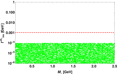
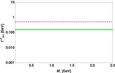
Figure 1: Left panel projects invisible width of Higgs ($H_{1}$) for $\sin\zeta<10^{-2}$ and right panel projects the same for $Z$ boson. Corresponding experimental upper limits Aaboud et al. (2019); Schael et al. (2006) are denoted by red horizontal dashed lines.

IV Dark matter

IV.1 Abundance

To compute the relic density of the light DM ($N_{-}$) via freeze-out mechanism, we use LanHEP Semenov (1996) and micrOMEGAs packages Pukhov et al. (1999); Belanger et al. (2007, 2009). The channels with lepton-anti lepton pair in final state ($\mu\overline{\mu}$, $\tau\overline{\tau}$, $\nu_{\mu}\overline{\nu_{\mu}}$, $\nu_{\tau}\overline{\nu_{\tau}}$) via $Z^{\prime}$ and $\eta$ portal contribute to relic density. Furthermore, SLQ portal t-channel processes with $d\overline{d}$, $s\overline{s}$ in the final state are also kinematically allowed. The key point is that the s-channel processes via light $Z^{\prime}$ provide a resonance in propagator, thereby meeting the Planck relic density value Aghanim et al. (2018) for the DM mass in the range $0.1-2.5$ GeV. The same is visible from left panel of Fig. 2, which projects relic density of DM with its mass. Right panel shows the $3\sigma$ Planck allowed region in $M_{Z^{\prime}}-M_{-}$ plane.

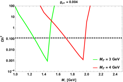
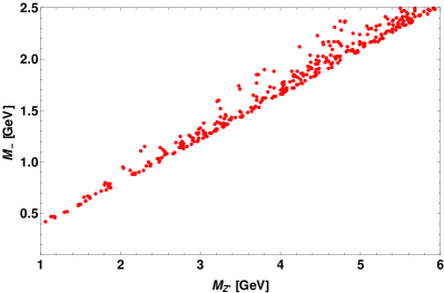
Figure 2: Behavior of relic density plotted against DM mass with black horizontal dotted lines denoting the $3\sigma$ range of Planck limit (Aghanim et al., 2018). Right panel corresponds to the parameter space consistent with $3\sigma$ allowed region of Planck data.

IV.2 Detection prospects

Moving to detection paradigm, SLQ portal spin-dependent (SD) cross section can arise from the effective interaction

$$\mathcal{L^{\rm SD}_{\rm eff}}\simeq\frac{y_{qR}^{2}\cos^{2}\beta}{4(M_{S_{1}}^{2}-M_{-}^{2})}\overline{N_{-}}\gamma^{\mu}\gamma^{5}N_{-}\overline{q}\gamma_{\mu}\gamma^{5}q\,.$$ (16)

The computed cross section is given by Agrawal et al. (2010)

$$\sigma_{\rm SD}=\frac{\mu_{r}^{2}}{\pi}\frac{\cos^{4}\beta}{(M_{S_{1}}^{2}-M_{-}^{2})^{2}}\left[y_{dR}^{2}\Delta_{d}+y_{sR}^{2}\Delta_{s}\right]^{2}J_{n}(J_{n}+1),$$ (17)

where $J_{n}=\frac{1}{2}$ stands for angular momentum, $\mu_{r}$ represents the reduced mass and the values of quark spin functions $\Delta_{q}$ are provided in (Agrawal et al., 2010). Fig. 3 projects the SD cross section and it is clear that it is well below the experimental upper limit from CDMSlite Agnese et al. (2018). Furthermore, the WIMP-nucleon cross section in gauge-portal (via $Z$, $Z^{\prime}$) and scalar-portal (via $H_{1}$, $H_{2}$) is found to be very small and insensitive to direct detection experiments.

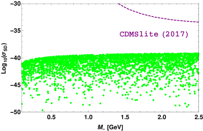
Figure 3: Spin-dependent WIMP-proton cross section as a function of DM mass in SLQ portal. Dashed line represent the bound levied by CDMSlite Agnese et al. (2018).

V Brief comments on neutrino mass

Neutrino mass can be obtained at one-loop level from the Yukawa interaction with $\eta$ in Eqn. (1). Assuming $(M^{2}_{\eta_{r}}+M^{2}_{\eta_{i}})/{2}=m_{0}^{2}$ is much greater than $M^{2}_{\eta_{r}}-M^{2}_{\eta_{i}}=\lambda^{\prime\prime}_{H\eta}v^{2}$, the expression for the radiatively generated neutrino mass Ma (2006); Vicente (2015) is given by

$$({\cal M}_{\nu})_{\beta\gamma}={\lambda^{\prime\prime}_{H\eta}v^{2}\over 32\pi^{2}}\sum_{i=1}^{3}{Y_{\beta i}Y_{\gamma i}\over M_{ii}}\left[{M_{ii}^{2}\over m_{0}^{2}-M_{ii}^{2}}+{M_{ii}^{4}\over(m_{0}^{2}-M^{2}_{ii})^{2}}\ln{M^{2}_{ii}\over m_{0}^{2}}\right],$$ (18)

where $M_{ij}={\rm diag}(M_{ee},M_{-},M_{+})$. For $m_{0}\sim 1$ TeV, $\lambda_{5}\sim 10^{-1}$ and $Y\sim 10^{-4}$, one can obtain neutrino mass at sub-eV scale. It should be noted that as the $L_{\mu}-L_{\tau}$ charges of SM leptons and the heavy fermions are same for each generation while the inert doublet is charged zero, the Yukawa matrix $Y$ is diagonal. Hence, the neutrino mass matrix (18) is diagonal by model construction, i.e., ${\cal M}_{\nu}={\rm diag}(m_{1},m_{2},m_{3})$, thus it can automatically accommodate the observed neutrino mixing angles, i.e., any unitary matrix can be used as the neutrino mixing matrix.

VI Constraints on new parameters from the flavor sector

Now, we look forward to constrain the model parameters of LQ and $Z^{\prime}$ couplings using the branching ratios of $B\to K\mu\mu$, $B\to K^{*}\mu\mu$, $B\to X_{s}\gamma$ decay modes and the recent measurements on lepton non-universality parameters, $R_{K^{(*)}}$.

VI.1 $b\to sll$

The general effective Hamiltonian mediating the $b\to sl^{+}l^{-}$ transition is given by Bobeth et al. (2000, 2002)

$${\cal H}_{\rm eff} = -\frac{4G_{F}}{\sqrt{2}}V_{tb}V_{ts}^{*}\Bigg{[}\sum_{i=1}^{6}C_{i}(\mu)O_{i}+\sum_{i=7,9,10}\Big{(}C_{i}(\mu)O_{i}+C_{i}^{\prime}(\mu)O_{i}^{\prime}\Big{)}\Bigg{]}\;,$$ (19)

where $G_{F}$ is the Fermi constant, $V_{qq^{\prime}}$ denote the CKM matrix elements, $C_{i}$’s stand for the Wilson coefficients evaluated at the renormalized scale $\mu=m_{b}$ Hou et al. (2014) and the values at NLL ($C_{9,10}$ values are calculated in the NNLL order) are listed in Table 3 .

$C_{1}$	$C_{2}$	$C_{3}$	$C_{4}$	$C_{5}$	$C_{6}$	$C_{7}^{\rm eff}$	$C_{8}^{\rm eff}$	$C_{9}$	$C_{10}$
$-3.001$	$1.008$	$-0.0047$	$-0.0827$	$0.0003$	$0.0009$	$-0.2969$	$-0.1642$	$4.2607$	$-4.2453$

Table 3: The SM Wilson coefficients computed at the scale $\mu=4.6$ GeV Hou et al. (2014).

Here $O_{i}$’s represent dimension-six operators responsible for leptonic/semileptonic processes, given as

$$O_{7}^{(\prime)} = \frac{e}{16\pi^{2}}\Big{[}\bar{s}\sigma_{\mu\nu}\left(m_{s}P_{L(R)}+m_{b}P_{R(L)}\right)b\Big{]}F^{\mu\nu},$$

$$O_{9}^{(\prime)} = \frac{\alpha_{\rm em}}{4\pi}(\bar{s}\gamma^{\mu}P_{L(R)}b)(\bar{l}\gamma_{\mu}l)\;,~{}~{}~{}~{}~{}~{}~{}O_{10}^{(\prime)}=\frac{\alpha_{\rm em}}{4\pi}(\bar{s}\gamma^{\mu}P_{L(R)}b)(\bar{l}\gamma_{\mu}\gamma_{5}l)\;,$$ (20)

with $\alpha_{\rm em}$ is the fine-structure constant, $P_{L,R}=(1\mp\gamma_{5})/2$ are the chiral operators and the values of primed Wilson coefficient are zero in the SM, but can be nonzero in the proposed $L_{\mu}-L_{\tau}$ model.

The one loop diagrams that provide non-zero contribution to the rare $b\to sll$ processes can take place via the exchange of $Z^{\prime},H_{1,2}$ one-loop penguin diagrams with SLQ and $N_{\pm}$ particles inside the loop as shown in Fig. 4 . The loop functions of second and third diagrams have $m_{q}M_{\pm}/M_{S_{1}}^{2}$ factor suppression, hence provide minimal contribution to $b\to sll$ processes. Thus, only the first diagram, mediated via $Z^{\prime}$ boson will contribute significantly to the $b\to sll$ channels.

Figure 4: One loop penguin diagrams that provide non-zero contribution to $b\to sll$ transitions in the present model.

In the presence of $Z^{\prime}$ exchanging one loop diagram, the transition amplitude of semileptonic $b\to sll$ decay process is given by Singirala et al. (2019)

$$\mathcal{M}=\frac{1}{2^{5}\pi^{2}}\frac{y_{qR}^{2}g_{\mu\tau}^{2}}{(q^{2}-M_{Z^{\prime}}^{2})}\mathcal{V}_{sb}(\chi_{-},\chi_{+})[\bar{u}(p_{B})\gamma^{\mu}(1+\gamma_{5})u(p_{K}))][\bar{v}(p_{2})\gamma_{\mu}u(p_{1}))],$$ (21)

which in comparison with the generalized effective Hamiltonian provides additional primed Wilson coefficient Singirala et al. (2019)

$$C_{9}^{\prime\rm NP}=\frac{\sqrt{2}}{2^{4}\pi G_{F}\alpha_{\rm em}V_{tb}V_{ts}^{*}}\frac{y_{qR}^{2}g_{\mu\tau}^{2}}{(q^{2}-{M_{Z^{\prime}}}^{2})}\mathcal{V}_{sb}\left(\chi_{-},\chi_{+}\right)\,.$$ (22)

to $b\to sll$ process. Here $p_{B},p_{K}$ and $p_{1,2}$ are the four momenta of initial $B$ meson, final $K$ meson and the charged leptons respectively. The detailed expression for the loop function $\mathcal{V}_{sb}(\chi_{-},\chi_{+})$ with $\chi_{\pm}=M_{\pm}^{2}/M_{S_{1}}^{2}$ is given in Appendix A Baek (2018); Hisano et al. (1996). Since there is only $C_{9}^{\prime\rm NP}$ in this model, the $B_{s}\to\mu\mu(\tau\tau)$ won’t play any role in constraining the new parameters.

$\boldsymbol{B\to Kl^{+}l^{-}}$

Including the new physics contribution, the differential branching ratio of $B\to Kll$ process in terms of $q^{2}$ is given by Bobeth et al. (2007)

$$\frac{d{\rm Br}}{dq^{2}}=\tau_{B}\frac{G_{F}^{2}\alpha_{\rm em}^{2}|V_{tb}V_{ts}^{*}|^{2}}{2^{8}\pi^{5}M_{B}^{3}}\sqrt{\lambda(M_{B}^{2},M_{K}^{2},q^{2})}\beta_{l}f_{+}^{2}\Big{(}a_{l}(q^{2})+\frac{c_{l}(q^{2})}{3}\Big{)}\;,$$ (23)

where

$$a_{l}(q^{2}) = q^{2}|F_{P}|^{2}+\frac{\lambda(M_{B}^{2},M_{K}^{2},q^{2})}{4}(|F_{A}|^{2}+|F_{V}|^{2})$$

$$+2m_{l}(M_{B}^{2}-M_{K}^{2}+q^{2}){\rm Re}(F_{P}F_{A}^{*})+4m_{l}^{2}M_{B}^{2}|F_{A}|^{2}\;,$$

$$c_{l}(q^{2}) = -\frac{\lambda(M_{B}^{2},M_{K}^{2},q^{2})}{4}\beta_{l}^{2}\left(|F_{A}|^{2}+|F_{V}|^{2}\right),$$ (24)

with

$$F_{V} = \frac{2m_{b}}{M_{B}}C_{7}^{\rm eff}+C_{9}^{\rm eff}+C_{9}^{\prime\rm NP},~{}~{}~{}~{}~{}F_{A}=C_{10}^{\rm SM},$$

$$F_{P} = m_{l}C_{10}^{\rm SM}\Big{[}\frac{M_{B}^{2}-M_{K}^{2}}{q^{2}}\Big{(}\frac{f_{0}(q^{2})}{f_{+}(q^{2})}-1\Big{)}-1\Big{]}\;,$$ (25)

and

$$\lambda(a,b,c)=a^{2}+b^{2}+c^{2}-2(ab+bc+ca),~{}~{}~{}~{}~{}\beta_{l}=\sqrt{1-4m_{l}^{2}/q^{2}}\;.$$ (26)

The detailed expression for $C_{7,9}^{\rm eff}$ Wilson coefficients Bobeth et al. (2011); Grinstein and Pirjol (2004); Bobeth et al. (2010) are presented in Appendix C. By using the lifetime of $B$ meson and masses of all the particles from Zyla et al. (2020), the $B\to K$ form factors from Colangelo et al. (1997), the predicted branching ratio values of $B\to K\mu\mu(\tau\tau)$ processes are

$${\rm Br}(B^{0}\to K^{0}\mu^{+}\mu^{-})\big{|}^{\rm SM}=(1.48\pm 0.12)\times 10^{-7}\,,$$ (27)

$${\rm Br}(B^{+}\to K^{+}\mu^{+}\mu^{-})\big{|}^{\rm SM}=(1.6\pm 0.13)\times 10^{-7}\,,$$ (28)

$${\rm Br}(B^{+}\to K^{+}\tau^{+}\tau^{-})\big{|}^{\rm SM}=(1.52\pm 0.121)\times 10^{-7}\,,$$ (29)

which in comparison with the corresponding experimental data Zyla et al. (2020)

$${\rm Br}(B^{0}\to K^{0}\mu^{+}\mu^{-})\big{|}^{\rm Expt}=(3.39\pm 0.34)\times 10^{-7}\,,$$ (30)

$${\rm Br}(B^{+}\to K^{+}\mu^{+}\mu^{-})\big{|}^{\rm Expt}=(4.41\pm 0.22)\times 10^{-7}\,,$$ (31)

$${\rm Br}(B^{+}\to K^{+}\tau^{+}\tau^{-})\big{|}^{\rm Expt}<2.25\times 10^{-3}\,,$$ (32)

can put constraints on $y_{qR},~{}g_{\mu\tau},~{}M_{-}$ and $M_{Z^{\prime}}$ parameters. As $Z^{\prime}$ does not couple to electrons, here we have considered only the channels with $\mu$ and $\tau$ in the final state.

$\boldsymbol{B\to K^{*}l^{+}l^{-}}$

The dilepton invariant mass spectrum for ${B}\rightarrow K^{*}l^{+}l^{-}$ decay after integration over all angles; $\theta_{l}$ (angle between $l^{-}$ and $B$ in the dilepton frame), $\theta_{K^{*}}$ (angle between $K^{-}$ and $B$ in the $K^{-}\pi^{+}~{}$ frame) and $\phi$ (angle between the normal of the $K^{-}\pi^{+}$ and the dilepton planes) Bobeth et al. (2008) is given by

$$\frac{d\Gamma}{dq^{2}}=\frac{3}{4}\left(J_{1}-\frac{J_{2}}{3}\right),~{}~{}~{}~{}~{}~{}J_{1,2}=2J_{1,2}^{s}+J_{1,2}^{c}\,,$$ (33)

where the detailed expressions for $J_{1,2}^{s(c)}$ as a function of transversity amplitudes are given as Altmannshofer et al. (2009b),

$$J^{s}_{1} = \frac{\left(2+\beta^{2}_{l}\right)}{4}\Bigg{[}|A_{\perp}^{L}|^{2}+|A_{\parallel}^{L}|^{2}+\left(L\rightarrow R\right)\Bigg{]}+\frac{4m^{2}_{l}}{q^{2}}{\rm Re}\left(A_{\perp}^{L}A_{\perp}^{R^{*}}+A_{\parallel}^{L}A_{\parallel}^{R^{*}}\right),~{}~{}$$

$$J^{c}_{1} = |A_{0}^{L}|^{2}+|A_{0}^{R}|^{2}+\frac{4m^{2}_{l}}{q^{2}}\Bigg{[}|A_{t}|^{2}+2{\rm Re}\left(A_{0}^{L}A_{0}^{R^{*}}\right)\Bigg{]},$$

$$J^{s}_{2} = \frac{\beta^{2}_{l}}{4}\left[|A_{\perp}^{L}|^{2}+|A_{\parallel}^{L}|^{2}+\left(L\rightarrow R\right)\right],$$

$$J^{c}_{2} = -\beta^{2}_{l}\left[|A_{0}^{L}|^{2}+\left(L\rightarrow R\right)\right],$$ (34)

with

$$A_{i}A_{j}^{*}=A_{i}^{L}\left(q^{2}\right)A^{*L}_{j}\left(q^{2}\right)+A_{i}^{R}\left(q^{2}\right)A^{*R}_{j}\left(q^{2}\right)\hskip 28.45274pt\left(i,j=0,\parallel,\perp\right),$$ (35)

in shorthand notation. The transversity amplitudes in terms of the form factors and (new) Wilson coefficients are given as Altmannshofer et al. (2009b)

$$A_{\perp L,R} = N\sqrt{2\lambda(M_{K^{*}}^{2},M_{B}^{2},q^{2})}\Big{[}\left((C_{9}^{\rm eff}+C_{9}^{\prime\rm NP})\mp C_{10}^{\rm SM}\right)\frac{V(q^{2})}{M_{B}+M_{K^{*}}}+\frac{2m_{b}}{q^{2}}C_{7}T_{1}(q^{2})\Big{]}\;,$$

$$A_{\parallel L,R} = -N\sqrt{2}(M_{B}^{2}-M_{K^{*}}^{2})\Big{[}\left((C_{9}^{\rm eff}-C_{9}^{\prime\rm NP})\mp C_{10}^{\rm SM}\right)\frac{A_{1}(q^{2})}{M_{B}-M_{K^{*}}}+\frac{2m_{b}}{q^{2}}C_{7}T_{2}(q^{2})\Big{]}\;,$$

$$A_{0L,R} = -\frac{N}{2M_{K^{*}}\sqrt{s}}\Big{[}\left(C_{9}^{\rm eff}-C_{9}^{\prime\rm NP})\mp C_{10}^{\rm SM}\right)$$

$$\times\left((M_{B}^{2}-M_{K^{*}}^{2}-q^{2})(M_{B}+M_{K^{*}})A_{1}(q^{2})-\lambda(M_{K^{*}}^{2},M_{B}^{2},q^{2})\frac{A_{2}(q^{2})}{M_{B}+M_{K^{*}}}\right)$$

$$+2M_{B}C_{7}\left((M_{B}^{2}+3M_{K^{*}}^{2}-q^{2})T_{2}(q^{2})-\frac{\lambda(M_{K^{*}}^{2},M_{B}^{2},q^{2})}{M_{B}^{2}-M_{K^{*}}^{2}}\right)\Big{]}\;,$$

$$A_{t} = 2N\sqrt{\frac{\lambda(M_{K^{*}}^{2},M_{B}^{2},q^{2})}{q^{2}}}C_{10}^{\rm SM}A_{0}(q^{2}),$$ (36)

where

$$N=V_{tb}V_{ts}^{*}\left[\frac{G_{F}^{2}\alpha_{\rm em}^{2}}{3\cdot 2^{10}\pi^{5}M_{B}^{3}}q^{2}\beta_{l}\sqrt{\lambda(M_{K^{*}}^{2},M_{B}^{2},q^{2})}\right]^{1/2}\;.$$ (37)

With the use of the mass and lifetime of particles from Particle Data Group Zyla et al. (2020) and the form factor from Ball and Zwicky (2005), the predicted branching ratios of $B\to K^{*}\mu\mu(\tau\tau)$ are

$${\rm Br}(B^{0}\to K^{*0}\mu^{+}\mu^{-})\big{|}^{\rm SM}=(1.967\pm 0.158)\times 10^{-8}\,,$$ (38)

$${\rm Br}(B^{+}\to K^{*+}\mu^{+}\mu^{-})\big{|}^{\rm SM}=(1.758\pm 0.141)\times 10^{-8}\,,$$ (39)

which in correlation with the corresponding experimental data Zyla et al. (2020)

$${\rm Br}(B^{0}\to K^{*0}\mu^{+}\mu^{-})\big{|}^{\rm Expt}=(9.4\pm 0.5)\times 10^{-7}\,,$$ (40)

$${\rm Br}(B^{+}\to K^{*+}\mu^{+}\mu^{-})\big{|}^{\rm Expt}<5.9\times 10^{-7}\,,$$ (41)

can constrain the $y_{qR},~{}g_{\mu\tau},~{}M_{-}$ and $M_{Z^{\prime}}$ parameters.

$\boldsymbol{R_{K^{(*)}}}$

Using the full Run-I and Run-II data set, recently the LHCb Collaboration has updated the lepton non-universality $R_{K}$ parameter in the $q^{2}\in[1,6]$ ${\rm GeV}^{2}$ Aaij et al. (2021)

$$R_{K}^{\rm LHCb21}\ =\ \frac{{\rm Br}(B^{+}\to K^{+}\mu^{+}\mu^{-})}{{\rm Br}(B^{+}\to K^{+}e^{+}e^{-})}=\ 0.846^{+0.042+0.013}_{-0.039-0.012}\$$ (42)

which is pretty much precise than the previous result Aaij et al. (2019)

$$R_{K}^{\rm LHCb19}\ =\ 0.846^{+0.060+0.016}_{-0.054-0.014}\,,$$ (43)

(where the first uncertainty is statistical and the second one is systematic), giving rise to the disagreement of $3.1\sigma$ from the SM prediction  Bobeth et al. (2007); Bordone et al. (2016)

$$R_{K}^{\rm SM}\ =\ 1.0003\pm 0.0001\,.$$ (44)

Equivalently, the recent measurements by the LHCb experiment on $R_{K^{*}}$ ratio in two bins of low-$q^{2}$ regions Aaij et al. (2017):

$$R_{K^{*}}^{\rm LHCb} \ =\ \begin{cases}0.660^{+0.110}_{-0.070}\pm 0.03\qquad q^{2}\in[0.045,1.1]~{}{\rm GeV}^{2}\,,\\ 0.69^{+0.11}_{-0.07}\pm 0.05\qquad q^{2}\in[1.1,6.0]~{}{\rm GeV}^{2}\,.\end{cases}$$ (45)

have respectively $2.1\sigma$ and $2.5\sigma$ deviations from their corresponding SM values Capdevila et al. (2018):

$$R_{K^{*}}^{\rm SM}\ =\ \begin{cases}0.92\pm 0.02\qquad q^{2}\in[0.045,1.1]~{}{\rm GeV}^{2}\,,\\ 1.00\pm 0.01\qquad q^{2}\in[1.1,6.0]~{}{\rm GeV}^{2}\,.\end{cases}$$ (46)

Additionally, though the Belle Collaboration has also announced measurements on $R_{K}$ Abdesselam et al. (2019a) and $R_{K^{*}}$ Abdesselam et al. (2019b) in several other bins, their results have comparatively larger uncertainties. The $R_{K^{(*)}}$ ratios can constrain all the four new parameters.

VI.2 $b\to s\gamma$

The $b\to s\gamma$ transition can occur at one loop level as shown in Fig. 5, where leptoquark and $N_{\pm}$ were driving in the loop.

Figure 5: One loop diagram of $b\to s\gamma$ processes in the proposed model.

$\boldsymbol{B\to X_{s}\gamma}$

In the presence of NP, the branching ratio of $B\to X_{s}\gamma$ decay process induced by the $b\to s\gamma$ transition is

$${\rm Br}(B\to X_{s}\gamma)={\rm Br}(B\to X_{s}\gamma)\big{|}^{\rm SM}\Bigg{(}1+\frac{C_{7}^{\gamma\prime\rm NP}}{C_{7}^{\gamma\rm SM}}\Bigg{)}^{2},$$ (47)

where

$$C_{7}^{\gamma\prime\rm NP}=-\frac{\sqrt{2}/3}{8G_{F}V_{tb}V_{ts}^{*}}\frac{y_{qR}^{2}}{M_{S_{1}}^{2}}\Big{(}J_{1}(\chi_{-})\cos^{2}\alpha+J_{1}(\chi_{+})\sin^{2}\alpha\Big{)},$$ (48)

with the loop functions $J_{1}(\chi_{\pm})$ Baek (2018)

$$J_{1}(\chi_{\pm})=\frac{1-6\chi_{\pm}+3\chi_{\pm}^{2}+2\chi_{\pm}^{3}-6\chi_{\pm}^{2}\log\chi_{\pm}}{12(1-\chi_{\pm})^{4}}\,.$$ (49)

The predicted SM branching ratio of $B\to X_{s}\gamma$ process Misiak et al. (2015)

$${\rm Br}(B\to X_{s}\gamma)\big{|}^{\rm SM}_{E_{\gamma}>1.6~{}{\rm GeV}}=(3.36\pm 0.23)\times 10^{-4}\,,$$ (50)

in relation with the corresponding experimental limit Amhis et al. (2017)

$${\rm Br}(B\to X_{s}\gamma)\big{|}^{\rm Expt}_{E_{\gamma}>1.6~{}{\rm GeV}}=(3.32\pm 0.16)\times 10^{-4}\,,$$ (51)

will impose constrain on the $y_{qR},~{}M_{-}$ parameters.

Due to the absence of $Z^{\prime}\mu\tau$ coupling in this model, the lepton flavor violating processes like $B\to K^{(*)}\mu\tau$, $\tau\to\mu\gamma$ and $\tau\to 3\mu$ are not allowed, thus couldn’t put bound on new parameters. Using Br($B\to K^{(*)}ll$) and $R_{K^{(*)}}$ observables, we show the $g_{\mu\tau},~{}M_{Z^{\prime}}$ allowed parameters space in the left panel of Fig. 6 . The region consistent with muon anomalous magnetic moment data is fully factored out by the constraint from the neutrino trident production. The validity of the effective field theory description in the present model lies above electroweak scale i.e., in the range $\sim(300-3000)$ GeV. It is indeed the favorable region of the ratio $M_{Z^{\prime}}/2g_{\mu\tau}$ and the lower values of this ratio is found to be excluded by various experimental searches, as projected in the plot.

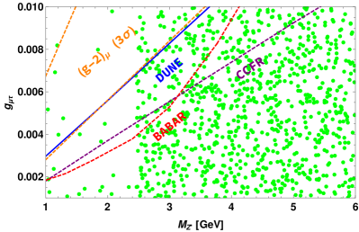
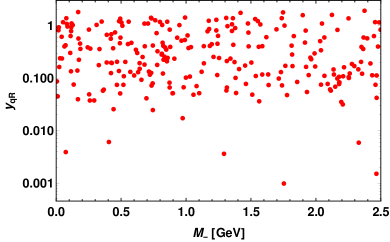
Figure 6: Constraints on $M_{Z}^{\prime}-g_{\mu\tau}$ (left panel) and $M_{-}-y_{qR}$ (right panel), obtained by using the branching ratios of $b\to sll$, $b\to s\gamma$ processes and the $R_{K^{(*)}}$ parameters. Lines in left panel denote the $3\sigma$ consistent region of muon $g-2$ Abi et al. (2021), exclusion limit from BABAR Lees et al. (2016), neutrino trident bounds from CCFR Mishra et al. (1991); Altmannshofer et al. (2014b) and DUNE Altmannshofer et al. (2019).

The $y_{qR},~{}M_{-}$ allowed region consistent with the Br($B\to K^{(*)}ll$), Br($B\to X_{s}\gamma$) and $R_{K^{(*)}}$ observables are presented in the right panel of Fig. 6 . The allowed range of all the four new parameters consistent with flavor phenomenology is given in Table 4 .

Parameters	$y_{qR}$	$g_{\mu\tau}$	$M_{-}$ (GeV)	$M_{Z^{\prime}}$ (GeV)
Allowed range	$0-2.0$	$0-0.01$	$0-2.5$	$1-6$

Table 4: The allowed regions of $y_{qR},~{}g_{\mu\tau},~{}M_{-}$ and $M_{Z^{\prime}}$ parameters.

VII Footprints on $b\to s+\displaystyle{\not}E$ decay modes

The SM treats neutrinos as the only carrier of missing energy in $b\to s$ transitions, i.e., the $b\to s+$ missing energy can be described by the $b\to s\nu\bar{\nu}$ decay modes in the SM. Here we consider the lepton flavor conserving $b\to s\nu_{l}\bar{\nu}_{l}$ processes. In the SM, the general effective Hamiltonian responsible for the $b\to s\nu_{l}\bar{\nu_{l}}$ transition is given by Altmannshofer et al. (2009a)

$$\mathcal{H}_{eff}=\frac{-4G_{F}}{\sqrt{2}}V_{tb}V_{ts}^{*}\left(C^{\nu}_{L}\mathcal{O}^{\nu}_{L}+C^{\nu}_{R}\mathcal{O}^{\nu}_{R}\right)+h.c.,$$ (52)

where

$$\mathcal{O}^{\nu}_{L}=\frac{\alpha_{\rm em}}{4\pi}\left(\bar{s}_{R}\gamma_{\mu}b_{L}\right)\left(\bar{\nu}\gamma^{\mu}\left(1-\gamma_{5}\right)\nu\right),\hskip 28.45274pt\mathcal{O}^{\nu}_{R}=\frac{\alpha_{\rm em}}{4\pi}\left(\bar{s}_{L}\gamma_{\mu}b_{R}\right)\left(\bar{\nu}\gamma^{\mu}\left(1-\gamma_{5}\right)\nu\right),$$ (53)

are the dimension-6 current-current operators with

$$C^{\nu}_{L}=-X(x_{t})/\sin^{2}\theta_{w}\;,~{}~{}~{}~{}X(x_{t})=X_{0}(x_{t})+\frac{\alpha_{s}}{4\pi}X_{1}(x_{t}),$$ (54)

being the SM Wilson coefficient. The expressions for ($X_{0,1}(x_{t})$ loop functions can be found in Ref. Misiak and Urban (1999); Buchalla and Buras (1999)). In the SM, the $C^{\nu}_{R}$ Wilson coefficient is absent but can be generated in some new physics models.

In our model, all possible diagrams contributing to $b\to s+\displaystyle{\not}E$ processes are shown in Fig. 7 . The first, third, fourth and fifth diagrams in Fig. 7, will be suppressed by the factor $m_{q}M_{\pm}/M_{S_{1}}^{2}$. In sixth diagram, the contributions of muon-neutrino and tau-neutrino cancel with each other in the leading order of NP due to their equal and opposite $L_{\mu}-L_{\tau}$ charge. Thus, only the $Z^{\prime}$ exchanging second diagram will contribute to $b\to s+\displaystyle{\not}E$ processes in addition to the SM $b\to s\nu_{l}\bar{\nu}_{l}$ modes.

Figure 7: One loop penguin diagrams that provide non-zero contribution for $b\to s+$ missing energy decay modes.

VII.1 $B\to K+\displaystyle{\not}E$

The total branching ratio of $B\to K+\displaystyle{\not}E$ decay is the sum of the branching ratio of semileptonic $B\to K$ decay with SM neutrino in the final state and the branching ratio of $B\to KN_{-}N_{-}$ decay, i.e.,

$${\rm Br}(B\to K+\displaystyle{\not}E)={\rm Br}(B\to K\nu\bar{\nu})+{\rm Br}(B\to KN_{-}N_{-}).$$ (55)

The branching ratio of $B\to K\nu_{l}\bar{\nu}_{l}$ decay process in the SM is given by Altmannshofer et al. (2009a)

$$\frac{d{\rm Br}}{ds_{B}}=\tau_{B}\frac{G_{F}^{2}\alpha^{2}}{256\pi^{5}}|V_{ts}^{*}V_{tb}|^{2}M_{B}^{5}\lambda^{3/2}(s_{B},\tilde{M}_{K}^{2},1)|f_{+}^{K}(s_{B})|^{2}|C_{L}^{\nu}|^{2},$$ (56)

where $\tilde{M}_{K}=M_{K}/M_{B},~{}s_{B}=s/M_{B}^{2}$. The predicted branching ratio values of $B^{+(0)}\to K^{+(0)}\nu_{l}\bar{\nu}_{l}$ by using input values from Zyla et al. (2020) and the corresponding experimental limits are tabulated in Table 5 .

The transition amplitude of $B\to KN_{-}N_{-}$ process from the $Z^{\prime}$ exchanging one loop penguin diagram is

$$\mathcal{M} = \frac{1}{2^{5}\pi^{2}}\frac{y_{bR}^{2}g_{\mu\tau}^{2}}{q^{2}-M_{Z^{\prime}}^{2}}\mathcal{V}_{sb}(\chi_{-},\chi_{+})[\bar{u}(p_{B})\gamma^{\mu}(1+\gamma_{5})u(p_{K}))][\bar{v}(p_{2})\gamma_{\mu}u(p_{1}))],$$ (57)

$$= C^{\rm NP}(q^{2})[\bar{u}(p_{B})\gamma^{\mu}(1+\gamma_{5})u(p_{K}))][\bar{v}(p_{2})\gamma_{\mu}u(p_{1}))]$$

where

$$C^{\rm NP}(q^{2})=\frac{1}{2^{5}\pi^{2}}\frac{y_{qR}^{2}g_{\mu\tau}^{2}\cos 2\beta\cos\alpha\sec\chi}{q^{2}-M_{Z^{\prime}}^{2}}\mathcal{V}_{sb}(\chi_{-},\chi_{+})\,,$$ (58)

and $p_{B}(p_{K})$ is the four momenta of $B(K)$ meson, $p_{1,2}$ are the momenta of $N_{-}$ fermion.

Using (57) , the branching ratio of $B\to KN_{-}N_{-}$ decay mode is given by

$$\frac{d{\rm Br}}{dq^{2}}=\tau_{B}\frac{1}{2^{7}\pi^{3}M_{B}^{3}}\sqrt{\lambda(M_{B}^{2},M_{K}^{2},q^{2})}\beta_{N}f_{+}^{2}\Big{(}a_{l}(q^{2})+\frac{c_{l}(q^{2})}{3}\Big{)}\;,~{}~{}~{}~{}$$ (59)

where

$$a_{l}(q^{2}) = q^{2}|F_{P}|^{2}+\left(\frac{\lambda(M_{B}^{2},M_{K}^{2},q^{2})}{4}+4M_{-}^{2}M_{B}^{2}\right)|F_{A}|^{2}+2M_{-}(M_{B}^{2}-M_{K}^{2}+q^{2}){\rm Re}(F_{P}F_{A}^{*})\;,$$

$$c_{l}(q^{2}) = -\frac{\lambda(M_{B}^{2},M_{K}^{2},q^{2})}{4}\beta_{N}^{2}|F_{A}|^{2},$$ (60)

with

$$F_{A}=C^{\rm NP}(q^{2}),~{}~{}F_{P}=M_{-}C^{\rm NP}(q^{2})\Big{[}\frac{M_{B}^{2}-M_{K}^{2}}{q^{2}}\Big{(}\frac{f_{0}(q^{2})}{f_{+}(q^{2})}-1\Big{)}-1\Big{]},~{}~{}\beta_{N}=\sqrt{1-4M_{-}^{2}/q^{2}}\,.~{}~{}~{}$$ (61)

$\boldsymbol{B\to K^{*}N_{-}N_{-}}$

Similary, the branching ratio of $B\to K^{*}+\displaystyle{\not}E$ is given by

$${\rm Br}(B\to K^{*}+\displaystyle{\not}E)={\rm Br}(B\to K^{*}\nu\bar{\nu})+{\rm Br}(B\to K^{*}N_{-}N_{-}).$$ (62)

The decay rate of $B\to K^{*}\nu\bar{\nu}$ decay mode in terms of $s_{B}$ and $\cos\theta$ is given as Altmannshofer et al. (2009a); Kim et al. (1999)

$$\frac{d^{2}\Gamma}{ds_{B}d\cos\theta}=\frac{3}{4}\frac{d\Gamma_{T}}{ds_{B}}\sin^{2}\theta+\frac{3}{2}\frac{d\Gamma_{L}}{ds_{B}}\cos^{2}\theta,$$ (63)

where the longitudinal and transverse polarization decay rates are

$$\frac{d\Gamma_{L}}{ds_{B}}=3M_{B}^{2}|A_{0}|^{2},\hskip 56.9055pt\frac{d\Gamma_{T}}{ds_{B}}=3M_{B}^{2}(|A_{\perp}|^{2}+|A_{\parallel}|^{2}),$$ (64)

with the transversity amplitudes, $A_{\perp,\parallel,0}$ in terms of form factor and Wilson coefficients are defined as

$$A_{\perp}(s_{B})=2N\sqrt{2}\lambda^{1/2}(1,\tilde{M}_{K*}^{2},s_{B})C_{L}^{\nu}\frac{V(s_{B})}{(1+\tilde{M}_{K^{*}})}\,,$$

$$A_{\parallel}(s_{B})=-2N\sqrt{2}(1+\tilde{M}_{K^{*}})C_{L}^{\nu}A_{1}(s_{B})\,,$$

$$A_{0}(s_{B})=-\frac{NC_{L}^{\nu}}{\tilde{M}_{K^{*}}\sqrt{s_{B}}}\left[(1-\tilde{M}_{K^{*}}^{2}-s_{B})(1+\tilde{M}_{K^{*}})A_{1}(s_{B})-\lambda(1,\tilde{M}_{K^{*}}^{2},s_{B})\frac{A_{2}(s_{B})}{1+\tilde{M}_{K^{*}}}\right],~{}~{}~{}$$ (65)

where $\tilde{M}_{K^{*}}=M_{K^{*}}/M_{B}$ and

$$N=V_{tb}V_{ts}^{*}\left[\frac{G_{F}^{2}\alpha^{2}M_{B}^{3}}{3\cdot 2^{10}\pi^{5}}s_{B}\lambda^{1/2}(1,\tilde{M}_{K^{*}}^{2},s_{B})\right]^{1/2}.$$ (66)

The same expression can be used for $B_{s}\to\phi\nu_{l}\bar{\nu}_{l}$. Now using all the required input values from Zyla et al. (2020), the $B_{(s)}\to K^{*}(\phi)$ form factor from Ball and Zwicky (2005), the branching ratio of $B_{(s)}\to K^{*}(\phi)\nu\bar{\nu}$ and their corresponding experimental limits are presented in Table 5 .

Decay process	BR in the SM	Experimental limit Zyla et al. (2020)
$B^{0}\to K^{0}\nu_{l}\bar{\nu}_{l}$	$(4.53\pm 0.267)\times 10^{-6}$	$\textless 2.6\times 10^{-5}$
$B^{+}\to K^{+}\nu_{l}\bar{\nu}_{l}$	$(4.9\pm 0.288)\times 10^{-6}$	$\textless 1.6\times 10^{-5}$
$B^{0}\to K^{*0}\nu_{l}\bar{\nu}_{l}$	$(9.48\pm 0.752)\times 10^{-6}$	$\textless 1.8\times 10^{-5}$
$B^{+}\to K^{*+}\nu_{l}\bar{\nu}_{l}$	$(1.03\pm 0.06)\times 10^{-5}$	$\textless 4.0\times 10^{-5}$
$B_{s}\to\phi\nu_{l}\bar{\nu}_{l}$	$(1.2\pm 0.07)\times 10^{-5}$	$\textless 5.4\times 10^{-3}$

Table 5: The predicted branching ratios of $B^{+(0)}\to M^{+(0)}\nu\bar{\nu}$ decays in the SM, where $M=K^{(*)},\phi$. Their corresponding experimental limits are also noted down in this table.

The decay rate of $B\to K^{*}N_{-}N_{-}$ process is given by

$$\frac{d\Gamma}{dq^{2}}=\frac{3}{4}\left(J_{1}-\frac{J_{2}}{3}\right),~{}~{}~{}~{}~{}~{}J_{1,2}=2J_{1,2}^{s}+J_{1,2}^{c}\,,$$ (67)

where

$$J^{s}_{1} = \frac{\left(2+\beta^{2}_{N}\right)}{4}\Bigg{[}|A_{\perp}^{L}|^{2}+|A_{\parallel}^{L}|^{2}+\left(L\rightarrow R\right)\Bigg{]}+\frac{4m^{2}_{N}}{q^{2}}{\rm Re}\left(A_{\perp}^{L}A_{\perp}^{R^{*}}+A_{\parallel}^{L}A_{\parallel}^{R^{*}}\right),~{}~{}$$

$$J^{c}_{1} = |A_{0}^{L}|^{2}+|A_{0}^{R}|^{2}+\frac{4M^{2}_{-}}{q^{2}}\Bigg{[}|A_{t}|^{2}+2{\rm Re}\left(A_{0}^{L}A_{0}^{R^{*}}\right)\Bigg{]},$$

$$J^{s}_{2} = \frac{\beta^{2}_{l}}{4}\left[|A_{\perp}^{L}|^{2}+|A_{\parallel}^{L}|^{2}+\left(L\rightarrow R\right)\right],$$

$$J^{c}_{2} = -\beta^{2}_{l}\left[|A_{0}^{L}|^{2}+\left(L\rightarrow R\right)\right],$$ (68)

with the transversity amplitudes in terms of the form factors and new functions are given as

$$A_{\perp L,R} = \mp N_{2}C^{\rm NP}(q^{2})\sqrt{2\lambda(M_{K^{*}}^{2},M_{B}^{2},q^{2})}\frac{V(q^{2})}{M_{B}+M_{K^{*}}}\;,$$

$$A_{\parallel L,R} = \pm N_{2}C^{\rm NP}(q^{2})\sqrt{2}(M_{B}^{2}-M_{K^{*}}^{2})\frac{A_{1}(q^{2})}{M_{B}-M_{K^{*}}}\;,$$

$$A_{0L,R} = \pm\frac{N_{2}C^{\rm NP}(q^{2})}{2M_{K^{*}}\sqrt{s}}\left((M_{B}^{2}-M_{K^{*}}^{2}-q^{2})(M_{B}+M_{K^{*}})A_{1}(q^{2})-\lambda(M_{K^{*}}^{2},M_{B}^{2},q^{2})\frac{A_{2}(q^{2})}{M_{B}+M_{K^{*}}}\right)\;,$$

$$A_{t} = 2N_{2}C^{\rm NP}(q^{2})\sqrt{\frac{\lambda(M_{K^{*}}^{2},M_{B}^{2},q^{2})}{q^{2}}}A_{0}(q^{2}),$$ (69)

and

$$N_{2}=\left[\frac{1}{3\cdot 2^{9}\pi^{3}M_{B}^{3}}q^{2}\beta_{N}\sqrt{\lambda(M_{K^{*}}^{2},M_{B}^{2},q^{2})}\right]^{1/2}\;.$$ (70)

For numerical estimation, we took the required input parameters like mass of particles, lifetime of $B_{(s)}$ meson, CKM parameters from Zyla et al. (2020) and the $B_{(s)}\to K^{*}(\phi)$ form factors from Ball and Zwicky (2005) . We have taken two different benchmark values of all the four new parameters, which are allowed by both the DM and flavor phenomenology, as presented in Table 6 .

Benchmark	$y_{qR}$	$g_{\mu\tau}$	$M_{-}$ (GeV)	$M_{Z^{\prime}}$ (GeV)
Benchmark-I	$2.0$	$0.002$	$1.7$	$4$
Benchmark-II	$2.0$	$0.008$	$1.8$	$4.8$

Table 6: Benchmark values of $y_{qR},~{}M_{-},~{}g_{\mu\tau}$ and $M_{Z^{\prime}}$ parameters used in our analysis.

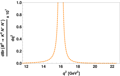
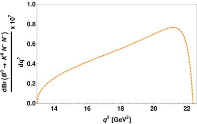
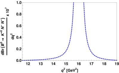
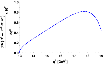
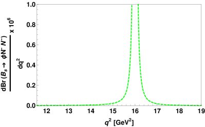
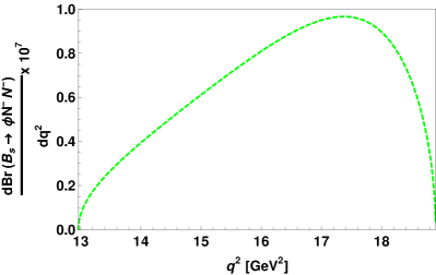
Figure 8: The branching ratios of $B^{0}\to K^{0}N_{-}N_{-}$ (left-top panel), $B^{0}\to K^{*0}N_{-}N_{-}$ (left-middle panel) and $B_{s}\to\phi N_{-}N_{-}$ (left-bottom panel) with respect to $q^{2}$ for Benchmark-I. The corresponding plots obtained by using the Benchmark-II are presented in the right panel.

By using all the discussed input parameters, we show the branching ratios of $B^{0}\to K^{0}N_{-}N_{-}$ (top panel), $B^{0}\to K^{*0}N_{-}N_{-}$ (middle panel) and $B_{s}\to\phi N_{-}N_{-}$ (bottom panel) with respect to $q^{2}$ in Fig. 8 . Here, the left panel figures are obtained by using the Benchmark-I values and the right panel plots are for Benchmark-II values. The estimated numerical values of the branching ratios of $b\to sN_{-}N_{-}$ processes for both sets of benchmark values are tabulated in Table 7 . For Benchmark-I, there is a singularity at $q^{2}=M_{Z^{\prime}}^{2}$, i.e., $q^{2}=16~{}{\rm GeV}^{2}$. In order to avoid the singularity, we put the cuts at $(M_{Z^{\prime}}-0.002)^{2}\leq q^{2}\leq(M_{Z^{\prime}}+0.002)^{2}$ ${\rm GeV}^{2}$.

Br($b\to sN_{-}N_{-}$)	Values using Benchmark-I	Values using Benchmark-II
Br($B^{0}\to K^{0}N_{-}N_{-}$)	$1.92\times 10^{-6}$	$4.1\times 10^{-7}$
Br($B^{+}\to K^{+}N_{-}N_{-}$)	$2.072\times 10^{-6}$	$2.6\times 10^{-7}$
Br($B^{0}\to K^{*0}N_{-}N_{-}$)	$3.23\times 10^{-6}$	$3.3\times 10^{-7}$
Br($B^{+}\to K^{*+}N_{-}N_{-}$)	$3.51\times 10^{-6}$	$3.61\times 10^{-7}$
Br($B_{s}\to\phi N_{-}N_{-}$)	$4.18\times 10^{-6}$	$3.93\times 10^{-7}$

Table 7: The predicted branching ratios of $b\to sN_{-}N_{-}$ processes for two different benchmark values of new parameters, which are compatible with both the dark matter and the flavor sectors.

In Table 8 , we present the branching ratios of $b\to s\displaystyle{\not}E$ which are the sum of the branching ratios of $b\to s\nu_{l}\bar{\nu}_{l}$ and $b\to sN_{-}N_{-}$ decay processes. We observe that, the addition of $b\to sN_{-}N_{-}$ process provide deviation from the SM predictions and are within the experimental limits.

Br($b\to s\displaystyle{\not}E$)	Benchmark-I	Benchmark-II	Experimental Limit Zyla et al. (2020)
Br($B^{0}\to K^{0}\displaystyle{\not}E$)	$0.645\times 10^{-5}$	$0.457\times 10^{-5}$	$<2.6\times 10^{-5}$
Br($B^{+}\to K^{+}\displaystyle{\not}E$)	$0.697\times 10^{-5}$	$0.516\times 10^{-5}$	$<1.6\times 10^{-5}$
Br($B^{0}\to K^{*0}\displaystyle{\not}E$)	$1.271\times 10^{-5}$	$0.981\times 10^{-5}$	$<1.8\times 10^{-5}$
Br($B^{+}\to K^{*+}\displaystyle{\not}E$)	$1.381\times 10^{-5}$	$1.066\times 10^{-5}$	$<4.0\times 10^{-5}$
Br($B_{s}\to\phi\displaystyle{\not}E$)	$1.618\times 10^{-5}$	$1.24\times 10^{-5}$	$<5.4\times 10^{-3}$

Table 8: The predicted branching ratios of $b\to s\displaystyle{\not}E$ processes for two different benchmark values of new parameters.

VIII Conclusion

In this work, we have investigated light GeV scale dark matter and flavor anomalies in a simple $U(1)_{L_{\mu}-L_{\tau}}$ variant with heavy neutral fermions and a $(\overline{3},1,1/3)$ scalar leptoquark. The $U(1)$ associated gauge boson ($Z^{\prime}$) plays a key role and is explored in the low mass regime. The lightest fermion is a stable dark matter and the resonance in $Z^{\prime}$ portal annihilation channels brings down the relic density to meet Planck data. WIMP-nucleon cross section of spin-dependent type is obtained in leptoquark portal and is looked up for consistency with CDMSlite bound. A benchmark is provided for generating light neutrino mass radiatively with small Yukawa.

We have constrained the new parameters by using the the branching ratios of $b\to sll$, $b\to s\gamma$ and the $R_{K^{(*)}}$ observables. We have taken two different sets of benchmark values of new parameters (which are compatible with both the dark matter and flavor phenomenology) and have shown the impact on rare $B$ meson decays to missing energy. There exist only experimental upper limits on the branching ratios of $b\to s+$missing energy processes. In the SM, the missing energy can be carried away by a pair of neutrino, i.e. by $b\to s\nu_{l}\bar{\nu}_{l}$ processes. We have assumed the missing energy part as a pair of dark matter in the proposed ${L_{\mu}-L_{\tau}}$ scenario. We have shown our prediction for the branching ratios of $b\to s\displaystyle{\not}E$ for two sets of benchmark values which are within the experimental limits. The observation of these modes at LHCb and Belle-II experiments would provide strong hints for the existence of light fermionic dark matter.

Appendix A Relevant vertices and couplings

Vertex	Coupling
$\overline{\mu}\,\gamma^{\mu}(c^{\mu}_{V}-c^{\mu}_{A}\gamma^{5})\mu Z_{\mu}$	$\frac{g}{2\cos\theta_{w}}(\cos\alpha-\sin\alpha\sin\theta_{w}\tan\chi)$
$\overline{\tau}\,\gamma^{\mu}(c^{\tau}_{V}-c^{\tau}_{A}\gamma^{5})\tau Z_{\mu}$	$\frac{g}{2\cos\theta_{w}}(\cos\alpha-\sin\alpha\sin\theta_{w}\tan\chi)$
$\overline{\nu_{\mu}}\,\gamma^{\mu}(c^{\nu_{\mu}}_{V}-c^{\nu_{\mu}}_{A}\gamma^{5})\nu_{\mu}Z_{\mu}$	$\frac{g}{2\cos\theta_{w}}(\cos\alpha-\sin\alpha\sin\theta_{w}\tan\chi)$
$\overline{\nu_{\tau}}\,\gamma^{\mu}(c^{\nu_{\tau}}_{V}-c^{\nu_{\tau}}_{A}\gamma^{5})\nu_{\tau}Z_{\mu}$	$\frac{g}{2\cos\theta_{w}}(\cos\alpha-\sin\alpha\sin\theta_{w}\tan\chi)$
$\overline{N_{-}}\gamma^{\mu}\gamma^{5}N_{-}Z_{\mu}$	$g_{\mu\tau}\cos 2\beta\sin\alpha\sec\chi$
$\overline{N_{+}}\gamma^{\mu}\gamma^{5}N_{+}Z_{\mu}$	$-g_{\mu\tau}\cos 2\beta\sin\alpha\sec\chi$
$\left(\overline{N_{-}}\gamma^{\mu}\gamma^{5}N_{+}+\overline{N_{+}}\gamma^{\mu}\gamma^{5}N_{-}\right)Z_{\mu}$	$g_{\mu\tau}\sin 2\beta\sin\alpha\sec\chi$
$\left(S_{1}\partial^{\mu}S_{1}^{\dagger}-S_{1}^{\dagger}\partial^{\mu}S_{1}\right)Z_{\mu}$	$\frac{g^{\prime}}{3}(-\cos\alpha\sin\theta_{w}+\sin\alpha\tan\chi)+g_{\mu\tau}\sin\alpha\sec\chi$
$\overline{\mu}\,\gamma^{\mu}\mu A_{\mu}$	$g\sin\theta_{w}$
$\overline{\tau}\,\gamma^{\mu}\tau A_{\mu}$	$g\sin\theta_{w}$
$\left(S_{1}\partial^{\mu}S_{1}^{\dagger}-S_{1}^{\dagger}\partial^{\mu}S_{1}\right)A_{\mu}$	$\frac{g^{\prime}}{3}\cos\theta_{w}$
$\overline{\mu}\,\gamma^{\mu}\mu Z^{\prime}_{\mu}$	$g_{\mu\tau}\cos\alpha\sec\chi$
$\overline{\tau}\,\gamma^{\mu}\tau Z^{\prime}_{\mu}$	-$g_{\mu\tau}\cos\alpha\sec\chi$
$\overline{\nu_{\mu}}\,\gamma^{\mu}(1-\gamma^{5})\nu_{\mu}Z^{\prime}_{\mu}$	$g_{\mu\tau}\cos\alpha\sec\chi$
$\overline{\nu_{\tau}}\,\gamma^{\mu}(1-\gamma^{5})\nu_{\tau}Z^{\prime}_{\mu}$	-$g_{\mu\tau}\cos\alpha\sec\chi$
$\overline{N_{-}}\gamma^{\mu}\gamma^{5}N_{-}Z^{\prime}_{\mu}$	-$g_{\mu\tau}\cos 2\beta\cos\alpha\sec\chi$
$\overline{N_{+}}\gamma^{\mu}\gamma^{5}N_{+}Z^{\prime}_{\mu}$	$g_{\mu\tau}\cos 2\beta\cos\alpha\sec\chi$
$\left(\overline{N_{-}}\gamma^{\mu}\gamma^{5}N_{+}+\overline{N_{+}}\gamma^{\mu}\gamma^{5}N_{-}\right)Z^{\prime}_{\mu}$	-$g_{\mu\tau}\sin 2\beta\cos\alpha\sec\chi$
$\left(S_{1}\partial^{\mu}S_{1}^{\dagger}-S_{1}^{\dagger}\partial^{\mu}S_{1}\right)Z^{\prime}_{\mu}$	$-\frac{g^{\prime}}{3}(\sin\alpha\sin\theta_{w}+\cos\alpha\tan\chi)-g_{\mu\tau}\cos\alpha\sec\chi$

Table 9: Fermion-gauge vertices and couplings.

Vertex	Coupling
$\overline{\mu}\mu H_{1}$	$\frac{m_{\mu}}{v}\cos\zeta$
$\overline{\tau}\tau H_{1}$	$\frac{m_{\tau}}{v}\cos\zeta$
$\overline{N^{c}_{-}}N_{-}H_{1}$	$-\frac{1}{\sqrt{2}}\left(f_{\mu}\cos^{2}\beta+f_{\tau}\sin^{2}\beta\right)\sin\zeta$
$\overline{N^{c}_{+}}N_{+}H_{1}$	$-\frac{1}{\sqrt{2}}\left(f_{\mu}\sin^{2}\beta+f_{\tau}\cos^{2}\beta\right)\sin\zeta$
$\overline{N^{c}_{-}}N_{+}H_{1}$	$-\frac{1}{\sqrt{2}}\left(f_{\mu}-f_{\tau}\right)\sin 2\beta\sin\zeta$
$S_{1}^{\dagger}S_{1}H_{1}$	$\lambda_{HS}v\cos\zeta-\lambda_{S\phi}v_{2}\sin\zeta$
$\overline{\mu}\mu H_{2}$	$\frac{m_{\mu}}{v}\sin\zeta$
$\overline{\tau}\tau H_{2}$	$\frac{m_{\tau}}{v}\sin\zeta$
$\overline{N^{c}_{-}}N_{-}H_{2}$	$\frac{1}{\sqrt{2}}\left(f_{\mu}\cos^{2}\beta+f_{\tau}\sin^{2}\beta\right)\cos\zeta$
$\overline{N^{c}_{+}}N_{+}H_{2}$	$\frac{1}{\sqrt{2}}\left(f_{\mu}\sin^{2}\beta+f_{\tau}\cos^{2}\beta\right)\cos\zeta$
$\overline{N^{c}_{-}}N_{+}H_{2}$	$\frac{1}{\sqrt{2}}\left(f_{\mu}-f_{\tau}\right)\sin 2\beta\cos\zeta$
$S_{1}^{\dagger}S_{1}H_{2}$	$\lambda_{HS}v\sin\zeta+\lambda_{S\phi}v_{2}\cos\zeta$
$\overline{d_{qR}^{c}}S_{1}N_{-}+{\rm{h.c.}}$	$y_{qR}\cos\beta$
$\overline{d_{qR}^{c}}S_{1}N_{+}+{\rm{h.c.}}$	$y_{qR}\sin\beta$

Table 10: Fermion-scalar vertices and couplings.

Appendix B Loop functions

The $b\to sll$ loop function, used in Section VI is given by

$$\mathcal{V}_{sb}(\chi_{-},\chi_{+}) = \sin^{2}2\beta\cos\alpha\sec\chi\left(1+4\sqrt{\chi_{-}\chi_{+}}j\left(\chi_{-},\chi_{+}\right)-2k\left(\chi_{-},\chi_{+}\right)\right)$$ (71)

$$+ 2(\sin^{2}\beta I(\chi_{+})+\cos^{2}\beta I(\chi_{-}))\cos^{2}\beta\cos\alpha\sec\chi\,,$$

where

$$f(\chi_{1},\chi_{2},\chi_{3},\cdots)\equiv\frac{f(\chi_{1},\chi_{3},\cdots)-f(\chi_{2},\chi_{3},\cdots)}{\chi_{1}-\chi_{2}},~{}~{}~{}~{}~{}~{}~{}~{}f=j,\kappa\,,$$ (72)

with

$$j(\chi) = \frac{\chi\log\chi}{\chi-1}\,,$$ (73)

$$\kappa(\chi) = \frac{\chi^{2}\log\chi}{\chi-1}\,,$$ (74)

$$I(\chi) = \frac{-3\chi^{2}+4\chi-1+2\chi^{2}\log\chi}{8(\chi-1)^{2}}\,.$$ (75)

Appendix C Effective Wilson coefficients

The effective $C_{7}^{\rm eff}$ and $C_{9}^{\rm eff}$ Wilson coefficients including the four-quark and gluon dipole operators, as mention in Eqn. (25) are given as Bobeth et al. (2011)

$$C_{7}^{\rm eff} = C_{7}-\frac{1}{3}\left[C_{3}+\frac{4}{3}C_{4}+20C_{5}+\frac{80}{3}C_{6}\right]+\frac{\alpha_{s}}{4\pi}\left[\left(C_{1}-6C_{2}\right)A(q^{2})-C_{8}F_{8}^{(7)}(q^{2})\right],~{}$$ (76)

$$C_{9}^{\rm eff} = C_{9}+h\left(0,q^{2}\right)\left[\frac{4}{3}C_{1}+C_{2}+\frac{11}{2}C_{3}-\frac{2}{3}C_{4}+52C_{5}-\frac{32}{3}C_{6}\right]$$ (77)

$$- \frac{1}{2}h\left(m_{b},q^{2}\right)\left[7C_{3}+\frac{4}{3}C_{4}+76C_{5}+\frac{64}{3}C_{6}\right]+\frac{4}{3}\left[C_{3}+\frac{16}{3}C_{5}+\frac{16}{9}C_{6}\right]$$

$$+ \frac{\alpha_{s}}{4\pi}\left[C_{1}\left(B(q^{2})+4C(q^{2})\right)-3C_{2}\left(2B\left(q^{2}\right)-C\left(q^{2}\right)\right)-C_{8}F_{8}^{(9)}\left(q^{2}\right)\right]$$

$$+ 8\frac{m^{2}_{c}}{q^{2}}\left[\left(\frac{4}{9}C_{1}+\frac{1}{3}C_{2}\right)(1+\lambda_{u})+2C_{3}+20C_{5}\right]\;,$$

where $\lambda_{u}=({V_{ub}V^{*}_{us}})/{(V_{tb}V^{*}_{ts})}$ and the functions $h(m_{i},q^{2})$ and $A,B,C,F_{8}^{(7,9)}$ can be found in Ref. Grinstein and Pirjol (2004); Bobeth et al. (2010).

References

- Zwicky (1937) F. Zwicky, Astrophys. J. 86, 217 (1937).
- Rubin and Ford (1970) V. C. Rubin and W. K. Ford, Jr., Astrophys. J. 159, 379 (1970).
- Clowe et al. (2004) D. Clowe, A. Gonzalez, and M. Markevitch, Astrophys. J. 604, 596 (2004), eprint astro-ph/0312273.
- Bertone et al. (2005) G. Bertone, D. Hooper, and J. Silk, Phys. Rept. 405, 279 (2005), eprint hep-ph/0404175.
- Arkani-Hamed et al. (2009) N. Arkani-Hamed, D. P. Finkbeiner, T. R. Slatyer, and N. Weiner, Phys. Rev. D 79, 015014 (2009), eprint 0810.0713.
- Dodelson and Widrow (1994) S. Dodelson and L. M. Widrow, Phys. Rev. Lett. 72, 17 (1994), eprint hep-ph/9303287.
- Zyla et al. (2020) P. A. Zyla et al. (Particle Data Group), PTEP 2020, 083C01 (2020).
- Sakharov (1991) A. Sakharov, Sov. Phys. Usp. 34, 392 (1991).
- Kolb and Wolfram (1980) E. W. Kolb and S. Wolfram, Nucl. Phys. B 172, 224 (1980), [Erratum: Nucl.Phys.B 195, 542 (1982)].
- Davidson et al. (2008) S. Davidson, E. Nardi, and Y. Nir, Phys. Rept. 466, 105 (2008), eprint 0802.2962.
- Buchmuller et al. (2005) W. Buchmuller, P. Di Bari, and M. Plumacher, Annals Phys. 315, 305 (2005), eprint hep-ph/0401240.
- Strumia (2006) A. Strumia, in Les Houches Summer School on Theoretical Physics: Session 84: Particle Physics Beyond the Standard Model (2006), pp. 655–680, eprint hep-ph/0608347.
- Aaij et al. (2014a) R. Aaij et al. (LHCb), Phys. Rev. Lett. 113, 151601 (2014a), eprint 1406.6482.
- Aaij et al. (2019) R. Aaij et al. (LHCb), Phys. Rev. Lett. 122, 191801 (2019), eprint 1903.09252.
- Aaij et al. (2021) R. Aaij et al. (LHCb) (2021), eprint 2103.11769.
- Bobeth et al. (2007) C. Bobeth, G. Hiller, and G. Piranishvili, JHEP 12, 040 (2007), eprint 0709.4174.
- Bordone et al. (2016) M. Bordone, G. Isidori, and A. Pattori, Eur. Phys. J. C76, 440 (2016), eprint 1605.07633.
- Aaij et al. (2017) R. Aaij et al. (LHCb), JHEP 08, 055 (2017), eprint 1705.05802.
- Capdevila et al. (2018) B. Capdevila, A. Crivellin, S. Descotes-Genon, J. Matias, and J. Virto, JHEP 01, 093 (2018), eprint 1704.05340.
- Amhis et al. (2019) Y. S. Amhis et al. (HFLAV) (2019), eprint 1909.12524, URL https://hflav.web.cern.ch.
- Na et al. (2015) H. Na, C. M. Bouchard, G. P. Lepage, C. Monahan, and J. Shigemitsu (HPQCD), Phys. Rev. D92, 054510 (2015), [Erratum: Phys. Rev.D93,no.11,119906(2016)], eprint 1505.03925.
- Fajfer et al. (2012a) S. Fajfer, J. F. Kamenik, and I. Nisandzic, Phys. Rev. D85, 094025 (2012a), eprint 1203.2654.
- Fajfer et al. (2012b) S. Fajfer, J. F. Kamenik, I. Nisandzic, and J. Zupan, Phys. Rev. Lett. 109, 161801 (2012b), eprint 1206.1872.
- Aaij et al. (2018) R. Aaij et al. (LHCb), Phys. Rev. Lett. 120, 121801 (2018), eprint 1711.05623.
- Wang et al. (2013) W.-F. Wang, Y.-Y. Fan, and Z.-J. Xiao, Chin. Phys. C37, 093102 (2013), eprint 1212.5903.
- Ivanov et al. (2005) M. A. Ivanov, J. G. Korner, and P. Santorelli, Phys. Rev. D71, 094006 (2005), [Erratum: Phys. Rev.D75,019901(2007)], eprint hep-ph/0501051.
- Abdesselam et al. (2019a) A. Abdesselam et al. (Belle) (2019a), eprint 1908.01848.
- Abdesselam et al. (2019b) A. Abdesselam et al. (Belle) (2019b), eprint 1904.02440.
- Aaij et al. (2013a) R. Aaij et al. (LHCb), Phys. Rev. Lett. 111, 191801 (2013a), eprint 1308.1707.
- Aaij et al. (2016) R. Aaij et al. (LHCb), JHEP 02, 104 (2016), eprint 1512.04442.
- Abdesselam et al. (2016) A. Abdesselam et al. (Belle), in LHC Ski 2016: A First Discussion of 13 TeV Results (2016), eprint 1604.04042.
- Aaij et al. (2014b) R. Aaij et al. (LHCb), JHEP 06, 133 (2014b), eprint 1403.8044.
- Aaij et al. (2013b) R. Aaij et al. (LHCb), JHEP 07, 084 (2013b), eprint 1305.2168.
- Badin and Petrov (2010) A. Badin and A. A. Petrov, Phys. Rev. D 82, 034005 (2010), eprint 1005.1277.
- Aslam and Lu (2009) M. J. Aslam and C.-D. Lu, Chin. Phys. C 33, 332 (2009), eprint 0802.0739.
- Aliev et al. (2007) T. M. Aliev, A. S. Cornell, and N. Gaur, JHEP 07, 072 (2007), eprint 0705.4542.
- Altmannshofer et al. (2009a) W. Altmannshofer, A. J. Buras, D. M. Straub, and M. Wick, JHEP 04, 022 (2009a), eprint 0902.0160.
- Kim and Wang (2008) C. S. Kim and R.-M. Wang, Phys. Rev. D 77, 094006 (2008), eprint 0712.2954.
- Jeon et al. (2006) J. H. Jeon, C. S. Kim, J. Lee, and C. Yu, Phys. Lett. B 636, 270 (2006), eprint hep-ph/0602156.
- Kim and Wang (2009) C. S. Kim and R.-M. Wang, Phys. Lett. B 681, 44 (2009), eprint 0904.0318.
- Sirvanli (2008) B. B. Sirvanli, Mod. Phys. Lett. A 23, 347 (2008), eprint hep-ph/0701173.
- Smith (2010) C. Smith, in 6th International Workshop on the CKM Unitarity Triangle (2010), eprint 1012.4398.
- Mahajan (2003) N. Mahajan, Phys. Rev. D 68, 034012 (2003).
- He et al. (1991a) X.-G. He, G. C. Joshi, H. Lew, and R. R. Volkas, Phys. Rev. D44, 2118 (1991a).
- He et al. (1991b) X. G. He, G. C. Joshi, H. Lew, and R. R. Volkas, Phys. Rev. D43, 22 (1991b).
- Ma et al. (2002) E. Ma, D. P. Roy, and S. Roy, Phys. Lett. B 525, 101 (2002), eprint hep-ph/0110146.
- Baek and Ko (2009) S. Baek and P. Ko, JCAP 10, 011 (2009), eprint 0811.1646.
- Altmannshofer et al. (2014a) W. Altmannshofer, S. Gori, M. Pospelov, and I. Yavin, Phys. Rev. D89, 095033 (2014a), eprint 1403.1269.
- Heeck et al. (2015) J. Heeck, M. Holthausen, W. Rodejohann, and Y. Shimizu, Nucl. Phys. B 896, 281 (2015), eprint 1412.3671.
- Crivellin et al. (2015) A. Crivellin, G. D’Ambrosio, and J. Heeck, Phys. Rev. Lett. 114, 151801 (2015), eprint 1501.00993.
- Fuyuto et al. (2016) K. Fuyuto, W.-S. Hou, and M. Kohda, Phys. Rev. D 93, 054021 (2016), eprint 1512.09026.
- Patra et al. (2016) S. Patra, W. Rodejohann, and C. E. Yaguna, JHEP 09, 076 (2016), eprint 1607.04029.
- Biswas et al. (2016) A. Biswas, S. Choubey, and S. Khan, JHEP 09, 147 (2016), eprint 1608.04194.
- Altmannshofer et al. (2016) W. Altmannshofer, S. Gori, S. Profumo, and F. S. Queiroz, JHEP 12, 106 (2016), eprint 1609.04026.
- Araki et al. (2017) T. Araki, S. Hoshino, T. Ota, J. Sato, and T. Shimomura, Phys. Rev. D 95, 055006 (2017), eprint 1702.01497.
- Chen and Nomura (2017) C.-H. Chen and T. Nomura, Phys. Rev. D 96, 095023 (2017), eprint 1704.04407.
- Chen and Nomura (2018) C.-H. Chen and T. Nomura, Phys. Lett. B 777, 420 (2018), eprint 1707.03249.
- Baek (2018) S. Baek, Phys. Lett. B781, 376 (2018), eprint 1707.04573.
- Bauer et al. (2018) M. Bauer, P. Foldenauer, and J. Jaeckel, JHEP 07, 094 (2018), eprint 1803.05466.
- Kamada et al. (2018) A. Kamada, K. Kaneta, K. Yanagi, and H.-B. Yu, JHEP 06, 117 (2018), eprint 1805.00651.
- Gninenko and Krasnikov (2018) S. N. Gninenko and N. V. Krasnikov, Phys. Lett. B 783, 24 (2018), eprint 1801.10448.
- Nomura and Okada (2018) T. Nomura and H. Okada, Phys. Rev. D 97, 095023 (2018), eprint 1803.04795.
- Banerjee and Roy (2019) H. Banerjee and S. Roy, Phys. Rev. D 99, 035035 (2019), eprint 1811.00407.
- Heeck et al. (2019) J. Heeck, M. Lindner, W. Rodejohann, and S. Vogl, SciPost Phys. 6, 038 (2019), eprint 1812.04067.
- Escudero et al. (2019) M. Escudero, D. Hooper, G. Krnjaic, and M. Pierre, JHEP 03, 071 (2019), eprint 1901.02010.
- Altmannshofer et al. (2019) W. Altmannshofer, S. Gori, J. Martín-Albo, A. Sousa, and M. Wallbank, Phys. Rev. D 100, 115029 (2019), eprint 1902.06765.
- Biswas and Shaw (2019) A. Biswas and A. Shaw, JHEP 05, 165 (2019), eprint 1903.08745.
- Kowalska et al. (2019) K. Kowalska, D. Kumar, and E. M. Sessolo, Eur. Phys. J. C 79, 840 (2019), eprint 1903.10932.
- Kang and Shigekami (2019) Z. Kang and Y. Shigekami, JHEP 11, 049 (2019), eprint 1905.11018.
- Joshipura et al. (2020) A. S. Joshipura, N. Mahajan, and K. M. Patel, JHEP 03, 001 (2020), eprint 1909.02331.
- Han et al. (2019) Z.-L. Han, R. Ding, S.-J. Lin, and B. Zhu, Eur. Phys. J. C 79, 1007 (2019), eprint 1908.07192.
- Jho et al. (2020) Y. Jho, S. M. Lee, S. C. Park, Y. Park, and P.-Y. Tseng, JHEP 04, 086 (2020), eprint 2001.06572.
- Amaral et al. (2020) D. W. P. d. Amaral, D. G. Cerdeno, P. Foldenauer, and E. Reid, JHEP 12, 155 (2020), eprint 2006.11225.
- Borah et al. (2020) D. Borah, S. Mahapatra, D. Nanda, and N. Sahu, Phys. Lett. B 811, 135933 (2020), eprint 2007.10754.
- Huang et al. (2021) G.-y. Huang, F. S. Queiroz, and W. Rodejohann, Phys. Rev. D 103, 095005 (2021), eprint 2101.04956.
- Borah et al. (2021) D. Borah, M. Dutta, S. Mahapatra, and N. Sahu (2021), eprint 2104.05656.
- Singirala et al. (2019) S. Singirala, S. Sahoo, and R. Mohanta, Phys. Rev. D 99, 035042 (2019), eprint 1809.03213.
- Georgi and Glashow (1974) H. Georgi and S. L. Glashow, Phys. Rev. Lett. 32, 438 (1974).
- Fritzsch and Minkowski (1975) H. Fritzsch and P. Minkowski, Annals Phys. 93, 193 (1975).
- Langacker (1981) P. Langacker, Phys. Rept. 72, 185 (1981).
- Georgi (1975) H. Georgi, AIP Conf. Proc. 23, 575 (1975).
- Pati and Salam (1974) J. C. Pati and A. Salam, Phys. Rev. D10, 275 (1974), [Erratum: Phys. Rev.D11,703(1975)].
- Pati and Salam (1973a) J. C. Pati and A. Salam, Phys. Rev. D8, 1240 (1973a).
- Pati and Salam (1973b) J. C. Pati and A. Salam, Phys. Rev. Lett. 31, 661 (1973b).
- Shanker (1982a) O. U. Shanker, Nucl. Phys. B206, 253 (1982a).
- Shanker (1982b) O. U. Shanker, Nucl. Phys. B204, 375 (1982b).
- Kaplan (1991) D. B. Kaplan, Nucl. Phys. B365, 259 (1991).
- Schrempp and Schrempp (1985) B. Schrempp and F. Schrempp, Phys. Lett. 153B, 101 (1985).
- Gripaios (2010) B. Gripaios, JHEP 02, 045 (2010), eprint 0910.1789.
- Alok et al. (2017) A. K. Alok, B. Bhattacharya, A. Datta, D. Kumar, J. Kumar, and D. London, Phys. Rev. D96, 095009 (2017), eprint 1704.07397.
- Bečirević and Sumensari (2017) D. Bečirević and O. Sumensari, JHEP 08, 104 (2017), eprint 1704.05835.
- Hiller and Nisandzic (2017) G. Hiller and I. Nisandzic, Phys. Rev. D96, 035003 (2017), eprint 1704.05444.
- D’Amico et al. (2017) G. D’Amico, M. Nardecchia, P. Panci, F. Sannino, A. Strumia, R. Torre, and A. Urbano, JHEP 09, 010 (2017), eprint 1704.05438.
- Bečirević et al. (2016) D. Bečirević, S. Fajfer, N. Košnik, and O. Sumensari, Phys. Rev. D94, 115021 (2016), eprint 1608.08501.
- Bauer and Neubert (2016) M. Bauer and M. Neubert, Phys. Rev. Lett. 116, 141802 (2016), eprint 1511.01900.
- Calibbi et al. (2015) L. Calibbi, A. Crivellin, and T. Ota, Phys. Rev. Lett. 115, 181801 (2015), eprint 1506.02661.
- Freytsis et al. (2015) M. Freytsis, Z. Ligeti, and J. T. Ruderman, Phys. Rev. D92, 054018 (2015), eprint 1506.08896.
- Dumont et al. (2016) B. Dumont, K. Nishiwaki, and R. Watanabe, Phys. Rev. D94, 034001 (2016), eprint 1603.05248.
- Doršner et al. (2016) I. Doršner, S. Fajfer, A. Greljo, J. F. Kamenik, and N. Košnik, Phys. Rept. 641, 1 (2016), eprint 1603.04993.
- de Medeiros Varzielas and Hiller (2015) I. de Medeiros Varzielas and G. Hiller, JHEP 06, 072 (2015), eprint 1503.01084.
- Dorsner et al. (2011) I. Dorsner, J. Drobnak, S. Fajfer, J. F. Kamenik, and N. Kosnik, JHEP 11, 002 (2011), eprint 1107.5393.
- Davidson et al. (1994) S. Davidson, D. C. Bailey, and B. A. Campbell, Z. Phys. C61, 613 (1994), eprint hep-ph/9309310.
- Saha et al. (2010) J. P. Saha, B. Misra, and A. Kundu, Phys. Rev. D81, 095011 (2010), eprint 1003.1384.
- Mohanta (2014) R. Mohanta, Phys. Rev. D89, 014020 (2014), eprint 1310.0713.
- Sahoo and Mohanta (2016a) S. Sahoo and R. Mohanta, New J. Phys. 18, 013032 (2016a), eprint 1509.06248.
- Sahoo and Mohanta (2016b) S. Sahoo and R. Mohanta, Phys. Rev. D93, 114001 (2016b), eprint 1512.04657.
- Sahoo and Mohanta (2016c) S. Sahoo and R. Mohanta, Phys. Rev. D93, 034018 (2016c), eprint 1507.02070.
- Sahoo and Mohanta (2015) S. Sahoo and R. Mohanta, Phys. Rev. D91, 094019 (2015), eprint 1501.05193.
- Kosnik (2012) N. Kosnik, Phys. Rev. D86, 055004 (2012), eprint 1206.2970.
- Chauhan et al. (2018) B. Chauhan, B. Kindra, and A. Narang, Phys. Rev. D97, 095007 (2018), eprint 1706.04598.
- Bečirević et al. (2018) D. Bečirević, I. Doršner, S. Fajfer, N. Košnik, D. A. Faroughy, and O. Sumensari, Phys. Rev. D98, 055003 (2018), eprint 1806.05689.
- Angelescu et al. (2018) A. Angelescu, D. Bečirević, D. A. Faroughy, and O. Sumensari, JHEP 10, 183 (2018), eprint 1808.08179.
- Sahoo and Mohanta (2017a) S. Sahoo and R. Mohanta, Eur. Phys. J. C 77, 344 (2017a), eprint 1705.02251.
- Sahoo and Mohanta (2016d) S. Sahoo and R. Mohanta, New J. Phys. 18, 093051 (2016d), eprint 1607.04449.
- Sahoo and Mohanta (2017b) S. Sahoo and R. Mohanta, J. Phys. G 44, 035001 (2017b), eprint 1612.02543.
- Sahoo and Bhol (2020) S. Sahoo and A. Bhol (2020), eprint 2005.12630.
- Faroughy (2019) D. A. Faroughy, SciPost Phys. Proc. 1, 021 (2019), eprint 1811.07582.
- Napsuciale et al. (2020) M. Napsuciale, S. Rodríguez, and H. Hernández-Arellano (2020), eprint 2009.10658.
- Hook et al. (2011) A. Hook, E. Izaguirre, and J. G. Wacker, Adv. High Energy Phys. 2011, 859762 (2011), eprint 1006.0973.
- Cline et al. (2014) J. M. Cline, G. Dupuis, Z. Liu, and W. Xue, JHEP 08, 131 (2014), eprint 1405.7691.
- Lees et al. (2016) J. P. Lees et al. (BaBar), Phys. Rev. D 94, 011102 (2016), eprint 1606.03501.
- Sirunyan et al. (2019) A. M. Sirunyan et al. (CMS), Phys. Lett. B 792, 345 (2019), eprint 1808.03684.
- Adachi et al. (2020) I. Adachi et al. (Belle-II), Phys. Rev. Lett. 124, 141801 (2020), eprint 1912.11276.
- Mishra et al. (1991) S. R. Mishra et al. (CCFR), Phys. Rev. Lett. 66, 3117 (1991).
- Altmannshofer et al. (2014b) W. Altmannshofer, S. Gori, M. Pospelov, and I. Yavin, Phys. Rev. Lett. 113, 091801 (2014b), eprint 1406.2332.
- Aaboud et al. (2019) M. Aaboud et al. (ATLAS), Phys. Rev. Lett. 122, 231801 (2019), eprint 1904.05105.
- Schael et al. (2006) S. Schael et al. (ALEPH, DELPHI, L3, OPAL, SLD, LEP Electroweak Working Group, SLD Electroweak Group, SLD Heavy Flavour Group), Phys. Rept. 427, 257 (2006), eprint hep-ex/0509008.
- Semenov (1996) A. V. Semenov (1996), eprint hep-ph/9608488.
- Pukhov et al. (1999) A. Pukhov, E. Boos, M. Dubinin, V. Edneral, V. Ilyin, D. Kovalenko, A. Kryukov, V. Savrin, S. Shichanin, and A. Semenov (1999), eprint hep-ph/9908288.
- Belanger et al. (2007) G. Belanger, F. Boudjema, A. Pukhov, and A. Semenov, Comput. Phys. Commun. 176, 367 (2007), eprint hep-ph/0607059.
- Belanger et al. (2009) G. Belanger, F. Boudjema, A. Pukhov, and A. Semenov, Comput. Phys. Commun. 180, 747 (2009), eprint 0803.2360.
- Aghanim et al. (2018) N. Aghanim et al. (Planck) (2018), eprint 1807.06209.
- Agrawal et al. (2010) P. Agrawal, Z. Chacko, C. Kilic, and R. K. Mishra (2010), eprint 1003.1912.
- Agnese et al. (2018) R. Agnese et al. (SuperCDMS), Phys. Rev. D 97, 022002 (2018), eprint 1707.01632.
- Ma (2006) E. Ma, Phys. Rev. D73, 077301 (2006), eprint hep-ph/0601225.
- Vicente (2015) A. Vicente (2015), eprint 1507.06349.
- Bobeth et al. (2000) C. Bobeth, M. Misiak, and J. Urban, Nucl. Phys. B574, 291 (2000), eprint hep-ph/9910220.
- Bobeth et al. (2002) C. Bobeth, A. J. Buras, F. Kruger, and J. Urban, Nucl. Phys. B630, 87 (2002), eprint hep-ph/0112305.
- Hou et al. (2014) W.-S. Hou, M. Kohda, and F. Xu, Phys. Rev. D90, 013002 (2014), eprint 1403.7410.
- Hisano et al. (1996) J. Hisano, T. Moroi, K. Tobe, and M. Yamaguchi, Phys. Rev. D53, 2442 (1996), eprint hep-ph/9510309.
- Bobeth et al. (2011) C. Bobeth, G. Hiller, and D. van Dyk, JHEP 07, 067 (2011), eprint 1105.0376.
- Grinstein and Pirjol (2004) B. Grinstein and D. Pirjol, Phys. Rev. D 70, 114005 (2004), eprint hep-ph/0404250.
- Bobeth et al. (2010) C. Bobeth, G. Hiller, and D. van Dyk, JHEP 07, 098 (2010), eprint 1006.5013.
- Colangelo et al. (1997) P. Colangelo, F. De Fazio, P. Santorelli, and E. Scrimieri, Phys. Lett. B395, 339 (1997), eprint hep-ph/9610297.
- Bobeth et al. (2008) C. Bobeth, G. Hiller, and G. Piranishvili, JHEP 07, 106 (2008), eprint 0805.2525.
- Altmannshofer et al. (2009b) W. Altmannshofer, P. Ball, A. Bharucha, A. J. Buras, D. M. Straub, and M. Wick, JHEP 01, 019 (2009b), eprint 0811.1214.
- Ball and Zwicky (2005) P. Ball and R. Zwicky, Phys. Rev. D 71, 014029 (2005), eprint hep-ph/0412079.
- Misiak et al. (2015) M. Misiak et al., Phys. Rev. Lett. 114, 221801 (2015), eprint 1503.01789.
- Amhis et al. (2017) Y. Amhis et al. (HFLAV), Eur. Phys. J. C77, 895 (2017), eprint 1612.07233.
- Abi et al. (2021) B. Abi et al. (Muon g-2), Phys. Rev. Lett. 126, 141801 (2021), eprint 2104.03281.
- Misiak and Urban (1999) M. Misiak and J. Urban, Phys. Lett. B 451, 161 (1999), eprint hep-ph/9901278.
- Buchalla and Buras (1999) G. Buchalla and A. J. Buras, Nucl. Phys. B 548, 309 (1999), eprint hep-ph/9901288.
- Kim et al. (1999) C. S. Kim, Y. G. Kim, and T. Morozumi, Phys. Rev. D 60, 094007 (1999), eprint hep-ph/9905528.