FERMILAB-TM-2753-AD

Modeling Transverse Space Charge effects in IOTA with pyORBIT

Abstract

The role and mitigation of space charge effects are important aspects of the beam physics research to be performed at the Integrable Optics Test Accelerator (IOTA) at Fermilab. The impact of nonlinear integrability (partial and complete) on space charge driven incoherent and coherent resonances will be a new feature of this accelerator and has the potential to influence the design of future low energy proton synchrotrons. In this report we model transverse space charge effects using the PIC code pyORBIT. First we benchmark the single particle tracking results against MADX with checks on symplecticity, tune footprints, and dynamic aperture in a partially integrable lattice realized with a special octupole string insert. Our space charge calculations begin with an examination of the 4D symplecticity. Short term tracking is done first with the initial bare lattice and then with a matching of the rms values with space charge. Next, we explore slow initialization of charge as a technique to establish steady state and reduce emittance growth and beam loss following injection into a mismatched lattice. We establish values of space charge simulation parameters so as to ensure numerical convergence. Finally, we compare the simulated space charge induced tune shifts and footprints against theory.

1 Introduction

The Fermilab Integrable Optics Test Accelerator (IOTA) is a storage ring for beam physics research. An important aspect of the research program is to explore the potential of integrable optics to mitigate deleterious effects of space charge in high intensity proton synchrotrons. In theory, integrable single particle dynamics eliminate resonances, providing stable motion over a wide tune range. In a beam, large betatron tune spread is known to be effective at suppressing instabilities. To the extent that desirable properties of integrable single particle motion persist in the presence of strong space charge, integrability may help to preserve stability in intense beams, but that remains to be verified.

The IOTA ring is currently operating with electrons in the energy range 100 - 150 MeV. At a later stage, experiments will be performed with protons at a kinetic energy of 2.5 MeV. By turning on/off special nonlinear inserts, the ring can be operated with either conventional or integrable optics. Space charge in the proton beam will be a determinant factor for beam stability. As in any other low energy proton synchrotron, both incoherent and coherent space charge effects will play a role. When the ring is configured with integrable optics, the impact of the perturbation due to space charge on properties associated with integrability needs to be understood. In this context, it is important to assess the capability and suitability of existing simulation codes. We report here on a variety of relevant validation tests that were performed using pyORBIT [1], a PIC code developed and maintained at ORNL and motivated by the need to simulate certain aspects of SNS.

IOTA proton parameters
Circumference	39.97 [m]
Kinetic Energy	2.5 [MeV]
Maximum bunch intensity /current	9$\times 10^{10}$ / 8 [mA]
Transverse normalized rms emittance	(0.3, 0.3) [mm-mrad]
Betatron tunes	(5.3, 5.3)
Natural chromaticities	(-8.2, -8.1)
Average transverse beam sizes (rms)	(2.22, 2.22) [mm]
Kinematic $\gamma$ / Transition $\gamma_{T}$	1.003 / 3.75
Rf voltage	400 [V]
Rf frequency / harmonic number	2.2 [MHz] / 4
Bucket wavelength	$\sim 10$ [m]
Bucket half height in $\Delta p/p$	3.72 $\times 10^{-3}$
rms bunch length	1.7 [m]
rms energy /momentum spread	1.05$\times 10^{-5}$ / 1.99 $\times 10^{-3}$
Beam pipe radius	25 [mm]
Bunch density	6.9 $\times 10^{14}$ [m-3]
Plasma period $\tau_{p}$	0.18 [$\mu$-sec] / 0.1 [turns]
Average Debye length $\lambda_{D}$	559 [$\mu$m]

Table 1: Machine and beam parameters of the IOTA proton ring

Parameters for the IOTA proton ring are presented in Table 1. The plasma period is included because it is a relevant time scale for initial emittance growth [2] mechanisms. For example, charge redistribution has the shortest time scale $\tau_{p}/4$ while rms mismatch or energy transfer between planes have a time scale of $\sim 10\tau_{p}$. Taking into account relativistic corrections, the plasma period is [3]:

$$\tau_{p}=2\pi\sqrt{\frac{\epsilon_{0}m_{0}\gamma^{3}}{ne^{2}}}$$ (1.1)

Here $\epsilon_{0}$ is the vacuum permittivity, $m_{0}$ is the proton mass and $n$ is the number density of the proton bunch. The volume of a Gaussian bunch with extent $\pm(3\sigma_{x},3\sigma_{y},3\sigma_{z})$ along the three axes is

$$V=\sigma_{x}\sigma_{y}\sigma_{z}\left(\int_{-3}^{3}\exp[-\frac{u^{2}}{2}]du\right)^{3}=(2\pi)^{3/2}[\mathrm{erf}(3/\sqrt{2})]^{3}\sigma_{x}\sigma_{y}\sigma_{z}$$ (1.2)

Substituting $\sigma_{x}=\sigma_{y}=2.2\;\text{mm}$ and $\sigma_{z}=1.7$ m we obtain $\tau_{p}=0.1$ turn, which suggests that initial emittance growth will occur on the scale of a single turn.

The Debye length $\lambda_{D}$ is [3]

$$\lambda_{D}=\frac{\sqrt{\langle v_{\perp}^{2}\rangle}\tau_{p}}{2\pi}=\sqrt{\frac{\epsilon_{0}\gamma^{2}k_{B}T_{\perp}}{e^{2}n}}$$ (1.3)

The temperature in the horizontal plane is

$$k_{B}T_{x}=m_{0}\gamma\langle v_{x}^{2}\rangle=m_{0}\gamma c^{2}(\gamma^{2}-1)\langle(x^{\prime})^{2}\rangle=m_{0}\gamma c^{2}(\gamma^{2}-1)\gamma_{x}\epsilon_{x}$$ (1.4)

where $\gamma_{x}$ is the lattice Twiss function and $\epsilon_{x}$ is the un-normalized emittance. Averaging this over the whole ring, we find the average temperature over the ring (see Appendix A)

$$\langle k_{B}T_{x}\rangle=m_{0}c^{2}(\gamma^{2}-1)\epsilon_{x,N}[\frac{-2Q_{x}^{\prime}}{R}]$$ (1.5)

where $Q_{x}^{\prime}$ is the natural horizontal chromaticity, $R$ is the machine radius and $\epsilon_{x,N}$ is the normalized emittance. This relation shows for example that the average transverse temperature in a circular machine depends on the natural chromaticity and ring radius. Substituting, we find that the average Debye length over the ring is

$$\langle\lambda_{D}\rangle=\sqrt{\left[\frac{\epsilon_{0}m_{0}c^{2}\gamma^{2}(\gamma^{2}-1)\epsilon_{\perp,N}}{e^{2}n}\right]\left[\frac{(-2Q_{\perp}^{\prime})}{R}\right]}$$ (1.6)

The first square bracket in this equation contains beam dependent variables while the second bracket isolates the machine dependent quantities. The Debye length sets the scale for the importance of space charge effects; the regime $\langle\lambda_{D}\rangle\ll$ beam radius is space charge dominated. Table 1 shows that with an average beam size of 2.2 mm and $\lambda_{D}=0.56$ mm, IOTA will be in the space charge dominated regime at full intensity.

2 Single-Particle Tracking

In this section, we aim to validate single-particle tracking in pyORBIT against MADX, a well-established and extensively tested code. To minimize discrepancies possibly introduced by subtle differences in the way distributed nonlinearities are modeled by the two codes, all sources of nonlinearity other than those confined to a special insert region are turned off. The insert region is initially populated with octupole magnets whose strengths vary in inverse proportion to $\beta^{3}(s)$; theoretically, the dynamics of this system is characterized by a single invariant. Later, the octupoles are replaced by special nonlinear magnets, making the optics (again, theoretically) fully integrable (two invariants). Good agreement between the codes provides confirmation that the lattice element sequence is both read in and interpreted in a consistent manner and that basic single particle motion is modeled correctly by pyORBIT.

2.1 Symplecticity Tests

In Hamiltonian mechanics, a transformation of the coordinates is said to be canonical if it preserves the form of Hamilton’s equations. A related result is that dynamical evolution is itself a succession of infinitesimal canonical transformations and therefore, the dynamical evolution from initial to final phase space coordinates is also a canonical transformation. It can shown that a canonical transformation must satisfy a local analytic condition, the so-called symplectic condition. Conversely, a transformation that satisfies the symplectic condition is canonical. The symplectic condition can be stated as follows:

$$\mathsf{J}^{T}\mathsf{S}\mathsf{J}=\mathsf{S}$$ (2.1)

where $J$ is the Jacobian matrix of the transformation. Assuming the transformation is defined by the dynamical evolution map ${\cal M}$ connecting the initial and final phase space coordinates ${\bf X}(s_{0})$ and ${\bf X}(s_{f})$ one has

$${\bf X}(s_{f})={\cal M}{\bf X}(s_{0})$$ (2.2)

$$J_{k\ell}=\frac{\partial X_{k}(s_{f})}{\partial X_{\ell}(s_{0})}$$ (2.3)

where ${\bf X}(s_{i})$ represents the initial phase space vector of canonical coordinates while $X_{k}(s_{i})$ denotes individual components of this vector. The symplectic matrix $\mathsf{S}$ is defined as

$$\mathsf{S}=\left(\begin{array}[]{cccc}\mathsf{s}&0&\cdots&0\\ 0&\mathsf{s}&\cdots&0\\ \vdots&\vdots&\ddots&\vdots\\ 0&0&\cdots&\mathsf{s}\end{array}\right)\;\;\mathsf{s}=\left(\begin{array}[]{cc}0&1\\ -1&0\end{array}\right)$$ (2.4)

Geometrically, the determinant of the Jacobian matrix represents the ratio between final and initial differential (oriented) phase space volumes enclosing corresponding points in phase space. Taking the determinant on both sides of 2.1, and using $\det(S)=1$, one finds $\det\,\mathsf{J}=\pm 1$. However, in the limit of a vanishingly small step along $s$ the dynamical transformation must converge to the identity $I$ i.e. $\lim_{s\to 0}\mathsf{J}=\mathsf{I}$, and one concludes that $\det\mathsf{J}=1$ i.e. the phase space volume is a dynamical invariant. This is the well-known Liouville’s theorem.

A matrix is called symplectic if it satisfies Eq. (2.1), known as the symplectic condition. While a unimodular Jacobian determinant is a necessary condition for symplecticity, it is not a sufficient test in phase space of dimensions higher than two. We apply both the determinant test and the full symplectic condition test Eq. (2.1) as measures of the deviation from symplecticity.

A residual deviation from exact symplecticity of the one-turn map computed by the code due to numerical round-off errors or approximations will translate into a long term violation of Liouville’s theorem. Therefore, for accurate long term simulation of the dynamics, the Jacobian determinant of the one-turn maps generated by a tracking code should be as close as possible to 1. The finite size representation of floating point numbers sets a minimum for the achievable deviation. Assuming 64-bit floating point representation (53-bit significance) the minimal deviation due to round-off is

$$|\det(\mathsf{J})-1|\simeq 10^{-14}$$

By tracking two or more test particles originating from closely neighboring points in phase space, one can compute partial derivatives using finite differences. Since the latter are approximations, deviations from the exact values of the partial derivatives will translate into larger apparent deviation from symplecticity. A rough error bound for the accuracy of the derivative may be obtained from Taylor’s theorem. For simple one-sided ( either forward or backward) differences

$$\frac{\Delta X}{h}=\frac{f(X+h)-f(h)}{h}=f^{\prime}+{\cal O}(h)$$ (2.5)

while for centered differences,

$$\frac{\Delta f}{h}=\frac{f(X+h)-f(X-h)}{2h}=f^{\prime}+{\cal O}(h^{2})$$ (2.6)

Assuming that the Jacobian matrix is diagonally dominant with diagonal entries near unity and off diagonal entries of magnitude $<<1$ it can be shown that

$$1-h<\det(\mathsf{J}+\mathsf{h})<(1+2h+nh^{2})^{n/2}$$ (2.7)

where $n$ is the matrix dimension and it is assumed that the magnitude of the error affecting all the Jacobian entries is about the same. On the basis of this bound, using centered differences and $h\sim 10^{-3}$, deviations from unity of the determinant on the order of $10^{-6}$ are to be expected; larger deviations would be indicative either of code issues (i.g. incorrectly computed map) or of the presence of chaotic motion.

The previous discussion has implicitly assumed well-behaved, smooth differentiable dynamical maps. It should be obvious that to the extent that maps associated with chaotic motion are not (practically) differentiable, the Jacobian determinant test is expected to fail in chaotic regions. In a typical accelerator the dynamics is smooth in the vicinity of the reference orbit. Chaotic motion is observed as one moves away from reference trajectory, where nonlinearity become increasingly significant. An abrupt deviation of the Jacobian determinant away from unity may be used to delineate the dynamic aperture boundary.

We now discuss the results of the symplectic tests of single particle tracking with pyorbit. Since this report is limited to 4D (transverse) space charge studies, we consider 4D symplectic tests both here and in a later Section where space charge is turned on3.1. To perform numerical tests of symplecticity, it is best to work in normalized Floquet canonical coordinates. The latter are defined as follows

$$\mathbf{X}=\left[\frac{x}{\sqrt{\beta_{x}}},\frac{(\beta_{x}x^{\prime}+\alpha_{x}x)}{\sqrt{\beta_{x}}},\frac{y}{\sqrt{\beta_{y}}},\frac{(\beta_{y}y^{\prime}+\alpha_{y}y)}{\sqrt{\beta_{y}}}\right]$$ (2.8)

In these coordinates, all components of ${\bf X}$ have dimension $[\sqrt{L}]$ and the elements of the Jacobian matrix $\mathsf{J}$ are dimensionless.

We first present results of the symplecticity tests for the linear lattice. Figure 1 shows the deviation from unity of $\det\mathsf{J}$ and the maximum norm $|\mathsf{J}^{T}\mathsf{S}\mathsf{J}-\mathsf{S}|$ as functions of the transverse amplitude for this linear lattice.

In both figures, the deviations are shown for three small increments (0.01, 0.001, 0.0001) of the initial amplitude.

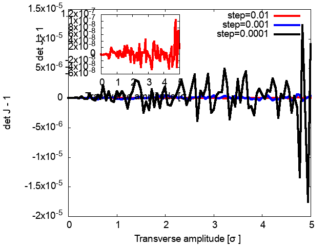
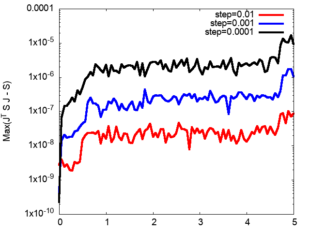
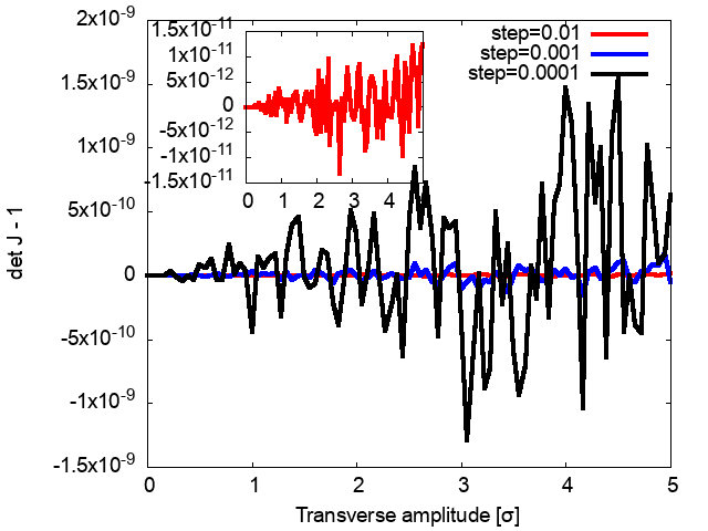
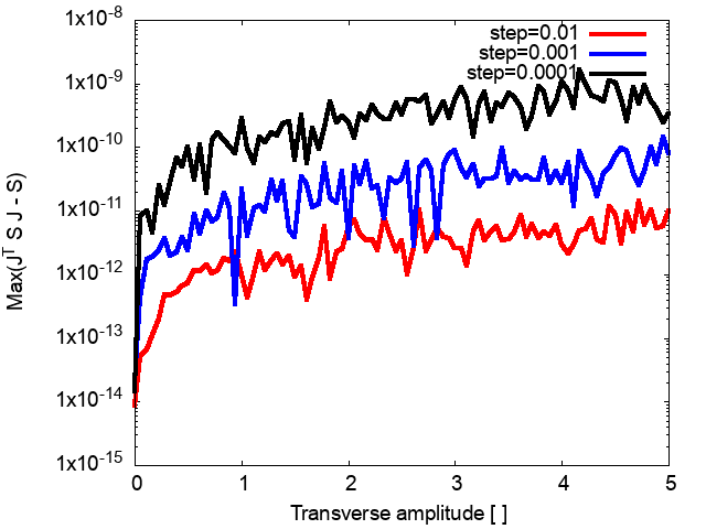
Figure 1: Linear lattice. Difference $|\det\mathsf{J}-1|$ (left) and maximum norm of the matrix $(\mathsf{J}^{T}\mathsf{S}\mathsf{J}-\mathsf{S})$ (right) as functions of the transverse amplitude in units of the rms beam size. Top: MADX, Bottom: pyORBIT. The left plot in both rows has insets showing the smallest values of the difference which result for the step size 0.01.

We find that the deviation from unity $\det\mathsf{J}-1$ is nearly $10^{-7}$ with MADX. For pyORBIT the deviation is at most 10^-11 for the at the largest step size of $0.01$ and increases for smaller step sizes. Similarly, the maximum norm $|\mathsf{J}^{T}\mathsf{S}\mathsf{J}-\mathsf{S}|$ is $\sim 10^{-8}$) with MADX and ($\sim 10^{-12}$) with pyORBIT for the step size $0.01$ and increases by an order of magnitude with each successive decrease in step size.o The larger deviation from unity of the Jacobian determinant observed with MADX appears to be related to its handling of dipole edge focusing, which is turned off in pyorbit.

Results for the lattice with the octupole string in IOTA are shown in Figure 2. Up to amplitudes of 4$\sigma$, $|\det[\mathsf{J}]-1|$ at step size $0.01$ is $\sim 10^{-8}$ with MADX and $\sim 10^{-4}$ with pyORBIT. The deviation increases steeply and is the largest at higher betatron amplitudes with both codes. For the smaller step of 0.001, the largest deviation over 0-5 $\sigma$ is $\sim 10^{-4}$ and can be considered the optimum step size; the deviations are larger again at the smaller step size 0.0001. The same pattern is observed for the maximum norm $|\mathsf{J}^{T}\mathsf{S}\mathsf{J}-\mathsf{S}|$.

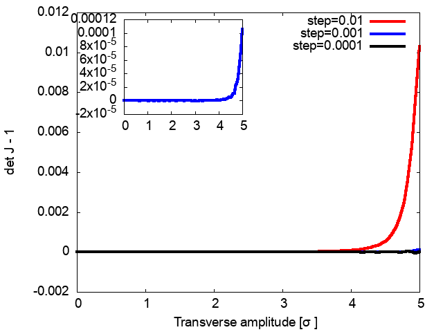
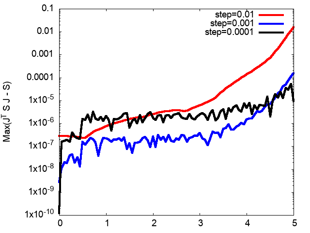
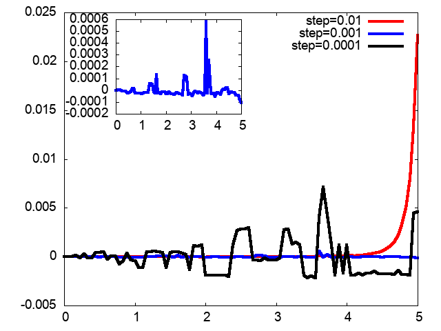
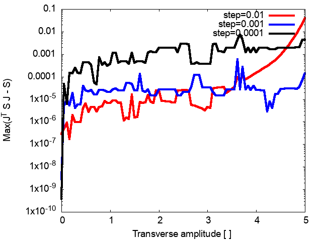
Figure 2: Lattice with octupoles. $(\det\mathsf{J}-1)$ (left) and maximum element of the matrix $\mathsf{J}^{T}\mathsf{S}\mathsf{J}-\mathsf{S}$ (right) as functions of the transverse amplitude in units of the rms beam size. Top: MADX, Bottom: pyORBIT

2.2 Tune Footprint

A meaningful way to validate pyORBIT against MADX is to compare tune footprints. To do so, particles are initialized uniformly from $(0,0,0,0)$ to $(5\sigma_{x},0,5\sigma_{y},0)$ in the $x$ and $y$ planes. They are then tracked for 5000 turns and the transverse positions $(x,y)$ of every particle are recorded for each turn at a fixed location. For each particle, the fractional part of the tunes $Q_{x}$ and $Q_{y}$ are obtained by performing a Fast Fourier Transform (FFT) of $x(n)$ and $y(n)$. $Q_{x}$ and $Q_{y}$ are presented as a scatter plot in tune space.

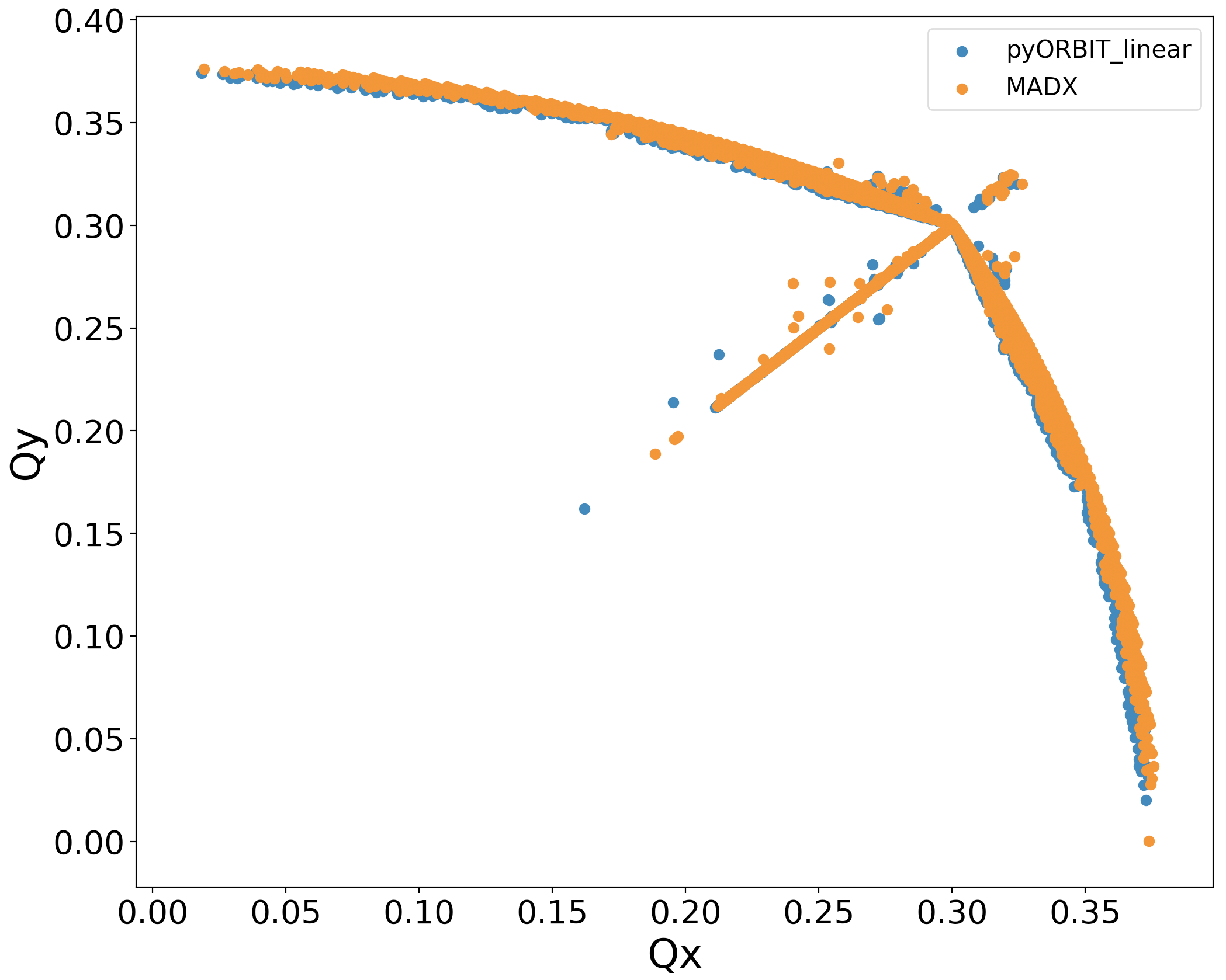
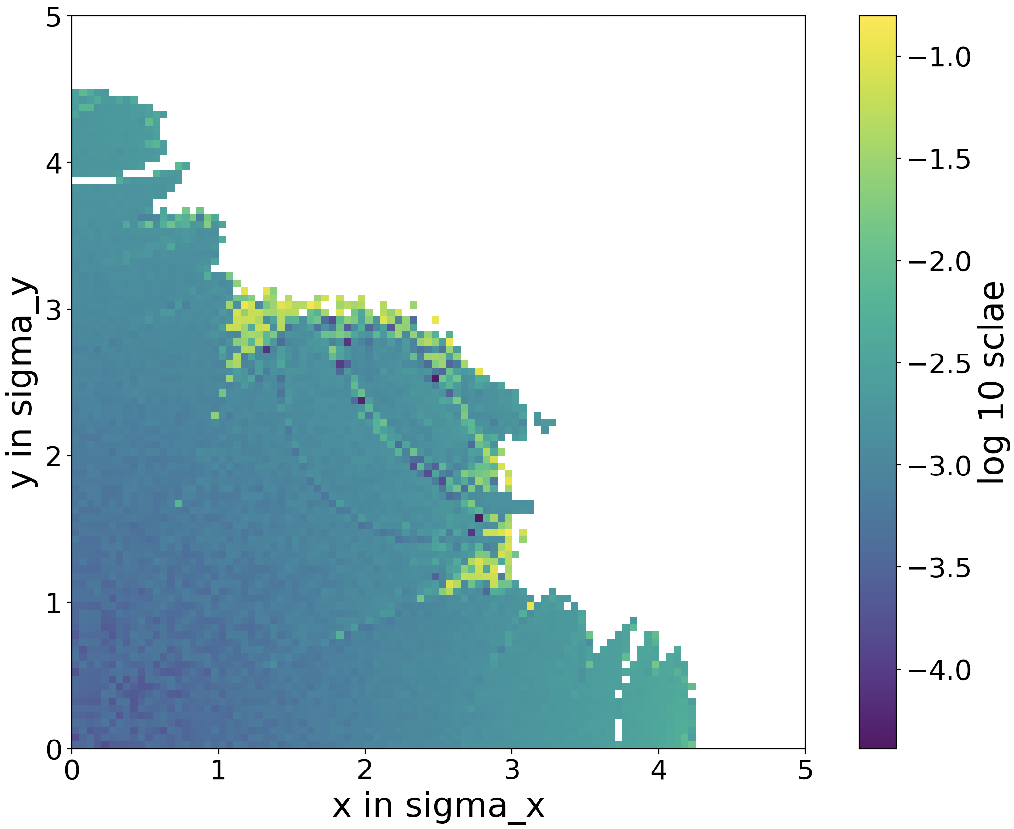
Figure 3: Left: Tune footprint of the IOTA lattice with octupoles, obtained with pyORBIT and MADX. Right: Difference in tune shifts (on a log scale) between pyORBIT and MADX as functions of the initial positions of the test particles.

The left plot in Figure 3 shows the tune footprint with octupoles added to the IOTA lattice. Both MADX and pyORBIT show a similar tune spread, which serves as a cross-check of the pyORBIT single particle tracking model. To make a more meaningful quantitative comparison between the codes, we present the difference in the tune shift computed by the two codes, and it is computed as

$$dQ=\mid Q_{x,P}-Q_{x,M}\mid+\mid Q_{y,P}-Q_{y,M}\mid$$ (2.9)

where e.g. $Q_{x,M},Q_{x,P}$ are the horizontal tunes calculated with MADX and pyORBIT respectively. The right plot in Figure 3 shows the tune difference $dQ$ for all test particles as functions of their initial positions. Figure 3b shows the tune difference $dQ$ for all test particles as function of their initial positions. For most test particles the difference between the tunes predicted by MADX and pyORBIT falls within the range $10^{-4}:10^{-3}$, which is comparable to the resolution of the FFT sampling. The result provides another confirmation of the correctness of single particle tracking in pyORBIT. Particles exhibiting the largest discrepancies are located close to the dynamic aperture boundary, as shown in Fig. 3. Beyond this boundary, the particles are lost and $\log dQ$ is undefined. All particles in the tune the footprint are initialized at coordinates $(x,0,y,0,0,0)$. The boundary defined by large deviations seen in Fig. 3 corresponds to the 4D dynamic aperture in Figure 4a. Small differences between the tune calculated by MADX and pyORBIT are likely due to increasingly unstable motion in the vicinity of the dynamic aperture boundary. We remark in passing that the fractal nature of this boundary is made evident by the tune difference diagram and that a similar procedure is used in a frequency map analysis except that in that case the same code is used to calculate tune differences between neighboring particles.

2.3 Dynamic Aperture Tests

The 4D, 5D and 6D dynamic apertures are calculated for the IOTA lattice with and without octupoles using both MADX and pyORBIT. Circular physical apertures with radius $25$ mm are assigned to all elements. $5000$ particles are initialized using one of the following procedures: The 4D dynamic aperture is calculated with the rf cavity turned off and particles are initialized at ($x_{i}$, 0, $y_{i}$, 0, 0, 0) so that the motion is restricted to transverse 4D phase space. The 5D dynamic aperture is calculated with the rf cavity turned off, and particles are initialized similarly but with a constant momentum offset of 1 $\sigma_{p}$ so that chromaticity can affect the dynamic aperture. The rf cavity is turned on for the 6D calculations with the same initial coordinates so that the effects of synchrotron motion are included.

A perfect lattice is used; no errors, e.g. field or alignment errors, are included. Particles are tracked for 10000 turns, and the initial coordinates in the $x$-$y$ plane of all surviving particles are recorded. The largest excursions of the surviving particles yield an upper bound of the dynamic aperture.

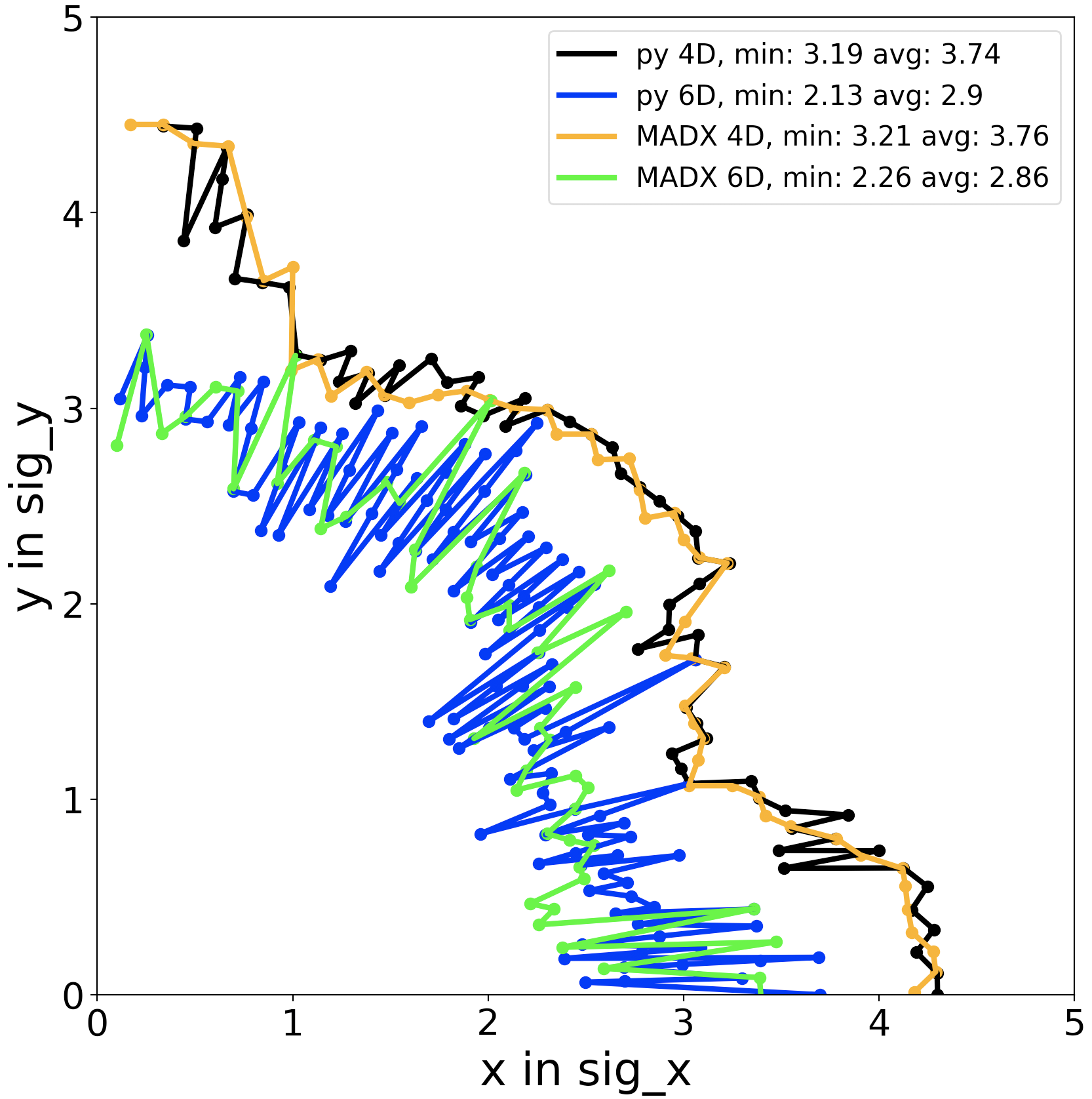
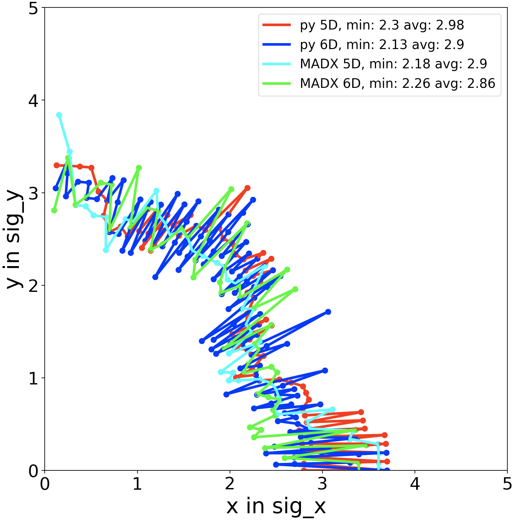
Figure 4: 4D, 5D, and 6D dynamic apertures (expressed in units of the rms beam sizes) for IOTA with octupoles from pyORBIT and MADX. Left: Comparison of 4D and 6D apertures, Right: Comparison of 5D and 6D apertures, they are nearly the same.

In the purely linear lattice, the horizontal dynamic aperture is approximately $5\sigma_{x}$ and $6\sigma_{y}$ vertically. As expected, the dynamic aperture is about the same as the physical aperture at the peak beta locations $\hat{\beta}_{x,y}$. Results from pyORBIT and MADX are in good agreement.

Results of dynamic aperture calculations with octupoles added to the linear lattice are shown in Figure 4 and summarized in Table 2 of minimum and average aperture sizes expressed in terms of rms beam sizes.

Aperture type	Minimum DA		Average DA
	pyORBIT	MADX	pyORBIT	MADX
$4$D	3.19	3.21	3.74	3.76
$5$D	2.3	2.18	2.98	2.9
$6$ D	2.13	2.26	2.9	2.86

Table 2: Minimum and average dynamic apertures with octupoles calculated using pyORBIT and MADX.

Referring to Table 2 and to Figure 4, there is good agreement between MADX and pyORBIT, providing additional confirmation of the soundness of the single particle tracking model in pyORBIT. The dynamic apertures for 6D and 5D tracking are generally much smaller than for 4D. For an emittance of 0.3$\mu m$ the latter is about 3 $\sigma$. This indicates that with a transverse Gaussian distribution, truncation at 3$\sigma$ should prevent particle loss. However, significant particle losses remain likely in the presence of space charge and for a more realistic lattice that includes alignment errors.

2.4 Hamiltonian Test

In the original paper on the integrable lattices [4] that provided the motivation for IOTA, the derivation assumes that in the absence of nonlinearity the $\beta$-function of the ring is symmetric i.e. $\beta_{x}(s)=\beta_{y}(s)=\beta(s)$ within the nonlinear insertion region. In principle this can be realized at low energy with radial transverse focusing provided by solenoids as this makes the beta function symmetric everywhere. However, as pointed out in the paper, the $\beta$-function symmetry requirement applies only within the nonlinear insertion region. With the nonlinearity confined to region $(s_{1},s_{2})$ the conditions $\beta_{x}(s_{1})=\beta_{y}(s_{1})=\beta_{x}(s_{2})=\beta_{y}(s_{2}))$ are sufficient to ensure this outcome. In IOTA, focusing in the linear portion of the ring is provided by quadrupoles. The optics is designed such that the map corresponding to that section is that of a thin axially symmetric lens. For purposes of analysis it is easier to assume ring-wide radial focusing; however to the extent that the $\beta$-function is symmetric within insertion region, the dynamics of the two situations is equivalent.

Expressed in terms of the independent variable $s$, the ring Hamiltonian has the analytical form [4]

$$H=\frac{1}{2}(p_{x}^{2}+p_{y}^{2})+\frac{k(s)}{2}(x^{2}+y^{2})+V(x,y,s)$$ (2.10)

where

$$k(s)=\begin{cases}0&s_{1}<s<s_{2}\\ k&\text{elsewhere}\end{cases}$$ (2.11)

is the linear radial focusing and $V(x,y,s)$ is a potential. The latter satisfies

$$V(x,y,s)=\begin{cases}V(x,y,s)&s_{1}<s<s_{2}\\ 0&\text{elsewhere}\end{cases}$$ (2.12)

i.e. it vanishes outside of the nonlinear insert. An octupole potential can be written as

$$V(s)=\frac{K_{3}(s)}{4!}[x^{4}+y^{4}-6x^{2}y^{2}],\;\;\;K_{3}=\frac{1}{(B\rho)}\frac{\partial^{3}B_{y}}{\partial x^{3}}$$ (2.13)

where the strength $K_{3}(s)$ (which has the definition as in MADX) varies with $s$. If the strength of each octupole in the string is chosen to vary as the inverse cube of the beta function in the section $s_{1}<s<s_{2}$ where $\beta_{x}(s)=\beta_{y}(s)=\beta(s)$ [4], then

$$K_{3}(s)=\kappa/\beta(s)^{3}$$ (2.14)

where $\kappa$ is a constant independent of $s$. Expressed in terms of Floquet coordinates $x_{N}==x/\sqrt{\beta_{x}},y_{N}==y/\sqrt{\beta_{y}}$, and transforming to the phase advance $\psi=\int\;ds/\beta(s)$ as the independent variable, the rescaled potential is

$$U=\beta(s)V((s)=\frac{1}{24}\kappa[x_{N}^{4}+y_{N}^{4}-6x_{N}^{2}y_{N}^{2}]$$ (2.15)

which is independent of the variable $\psi$.

Strictly speaking a purely transverse potential with a smooth longitudinal variation is not physically realizable; however, it can be reasonably well-approximated by a string of octupole magnets of different apertures; for that purpose, the IOTA octupole insert design uses 17 equally spaced magnets.

Figure 5 shows the $\beta$-functions in the IOTA ring; the octupoles occupy the 1.7 m section from $s=33$ m to $s=35$ m. The use of a sequence of discrete magnets is expected to result in small fluctuations of the idealized invariant Hamiltonian. Lattice imperfections in the linear part of the ring causing violations of the condition $\beta_{x}=\beta_{y}$ within the nonlinear insert region will have a similar effect.

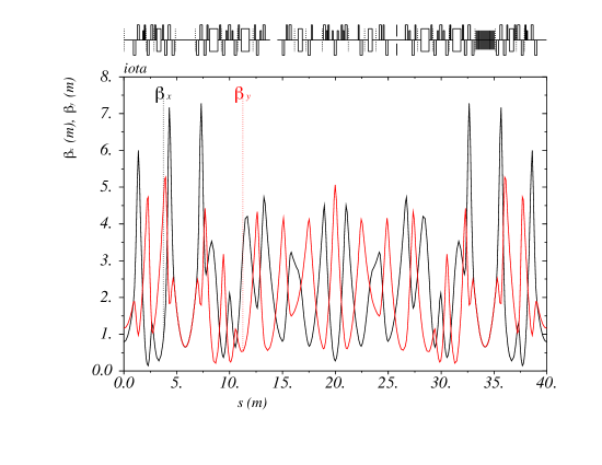
Figure 5: Beta functions in the IOTA ring; the octupoles are in the region from 33.3 to 35m.

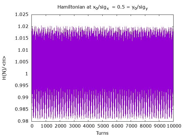
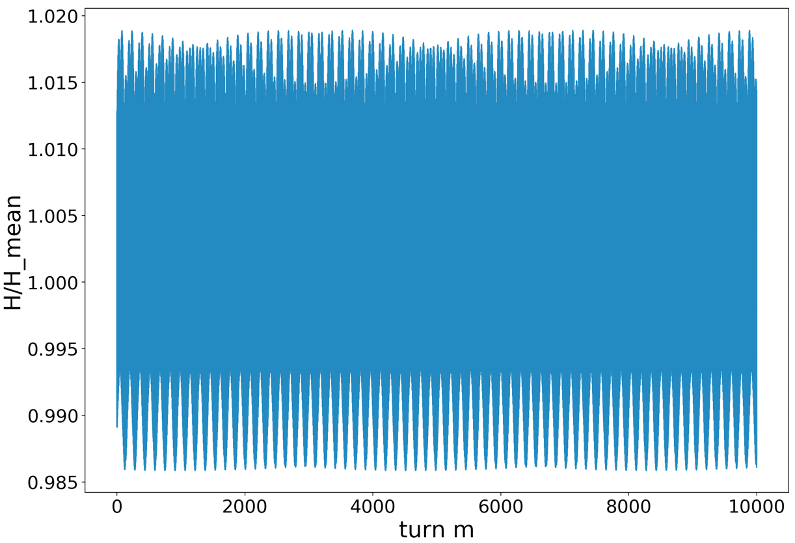
Figure 6: Variation in the single particle Hamiltonian relative to its initial value in MADX (left) and pyORBIT (right). Initial coordinates are $x/\sigma_{x}=0.5=y/\sigma_{y}$, $x^{\prime}=0=y^{\prime}$.

Figure 6 shows that the relative variation of the Hamiltonian invariant for a small amplitude particle predicted by both MADX and pyORBIT is approximately $\pm 2\%$. This variation increases for larger amplitudes and both codes remain in agreement.

3 pyORBIT Space Charge Model

pyORBIT is a particle-in-cell code in which macro-particles represent charged particles in a bunch. The macroparticles are deposited on a grid and a smoothed density is extracted by interpolation between the grid points. The electric potential is found by numerically solving Poisson’s equation in the beam rest frame which thereby allows evaluation of the space charge forces on the macro-particles. The details of the physical (as opposed to numerical) space charge force depend on the bunch intensity, the particle distribution and boundary conditions. In this report we consider only the transverse space charge forces and we assume open boundary conditions. The transverse distributions are assumed to be Gaussian since that is experimentally well-founded. The transverse forces vary along the bunch length due to the change in local density, so the longitudinal distribution also matters.

In our simulations, a waterbag distribution is used in the longitudinal plane. To prevent particles leaking out of the bucket when longitudinal space charge forces (to be reported in a separate study) are considered, particles are uniformly distributed within an inner Hamiltonian contour inside the separatrix defined by the RF cavity. An example using $10^{6}$ macro-particles is plotted in Figure 8.

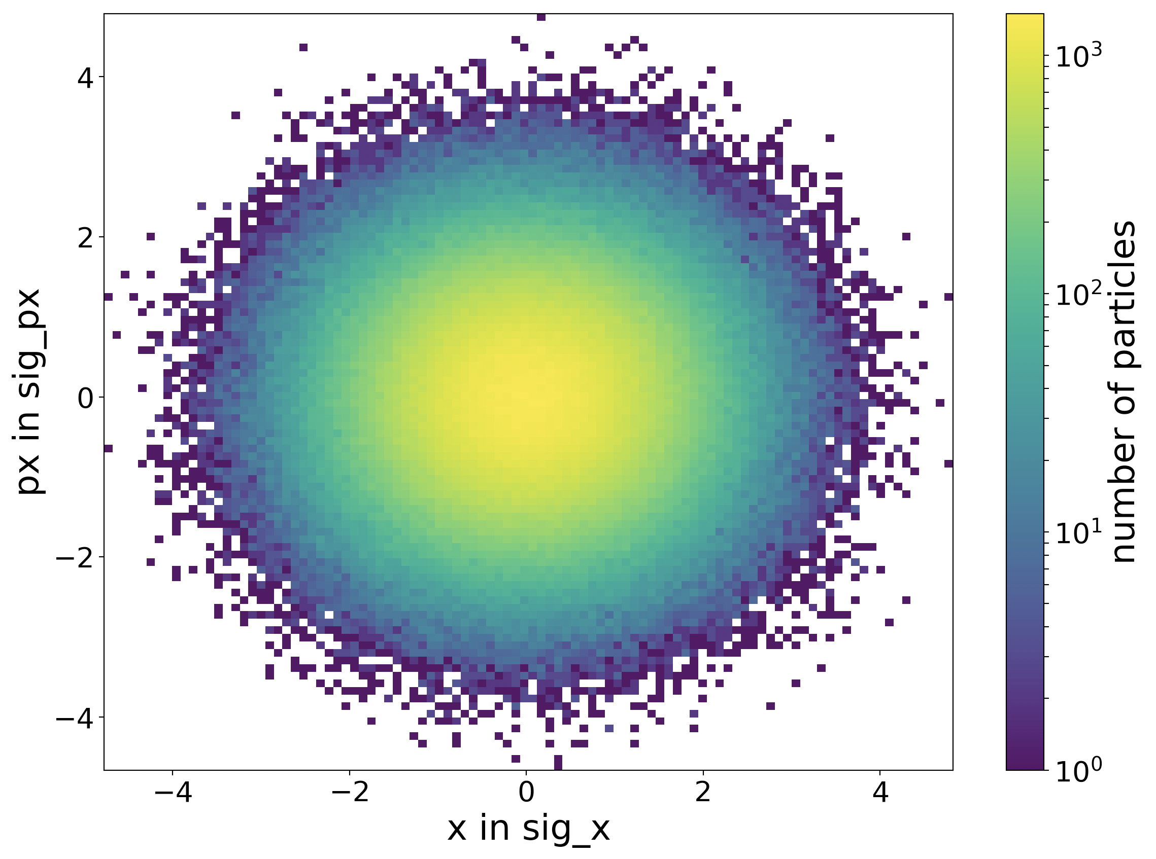
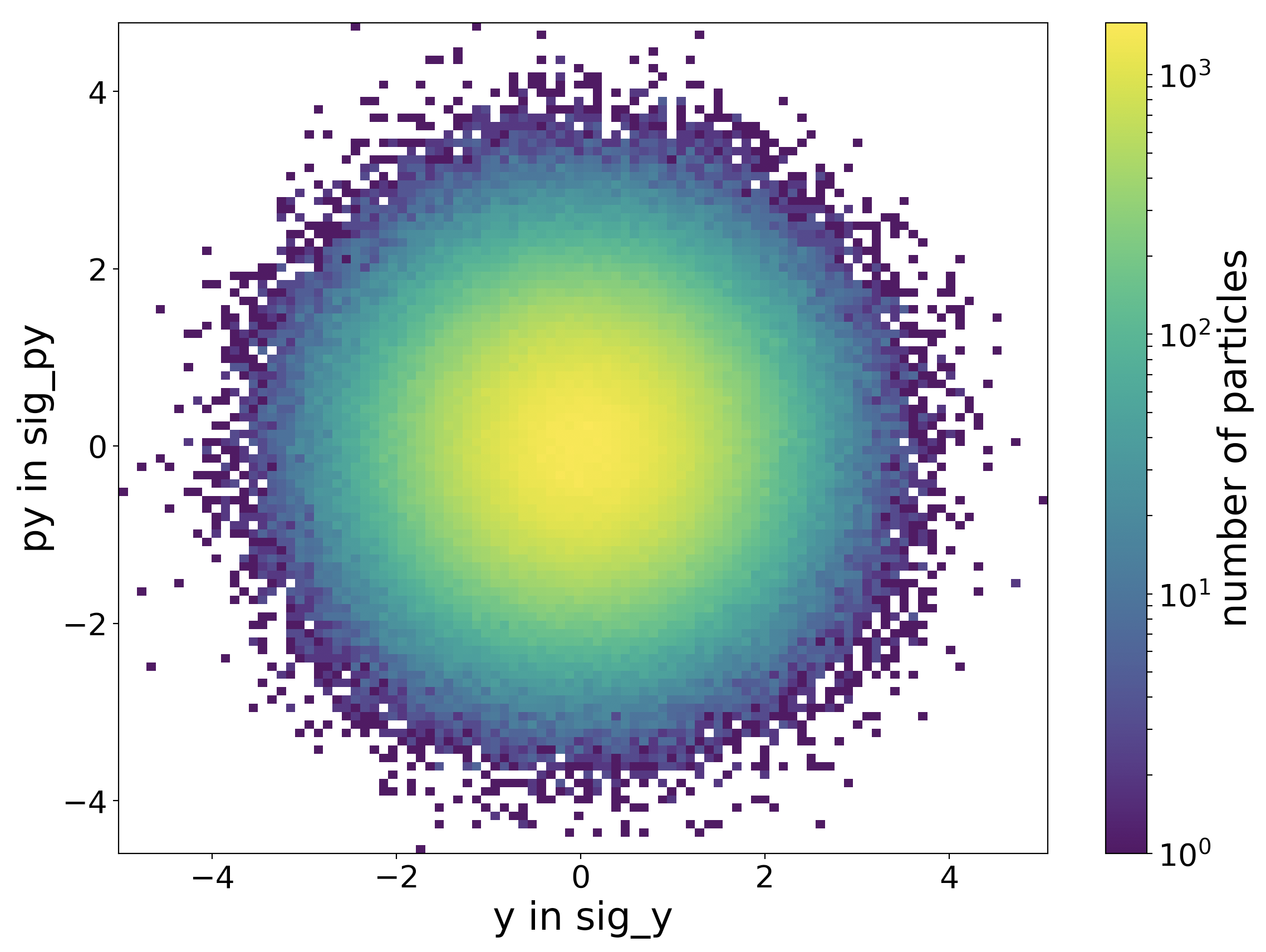
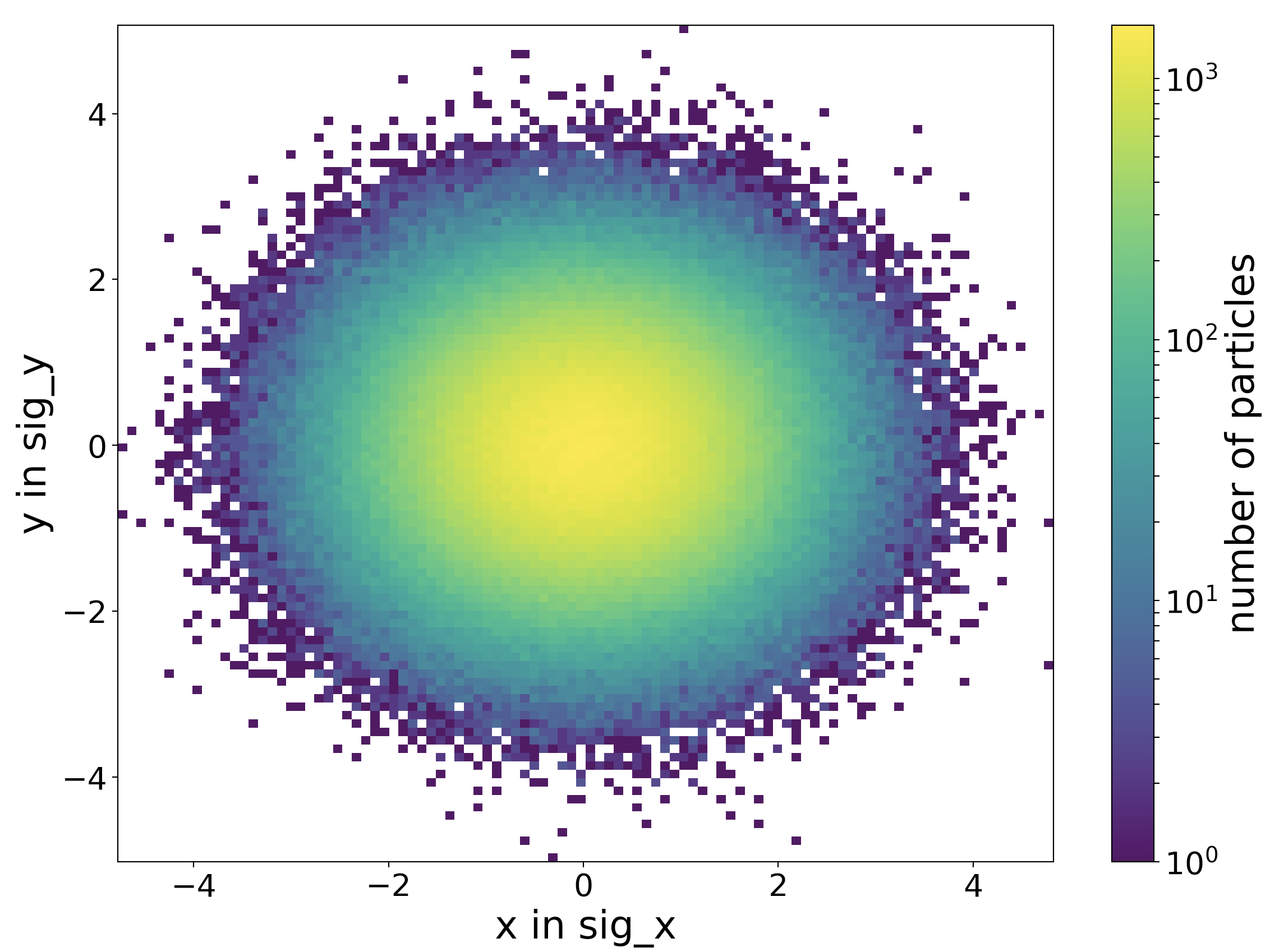
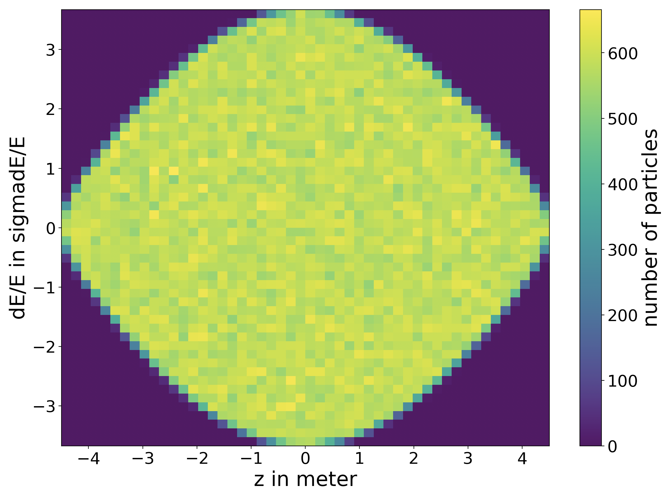
Figure 7: Particle distribution in x-pz (left) and y-py plane (right)

Figure 8: Particle distribution in x-y (eft) and z-dE plane (right)

3.1 Symplectic tests with space charge

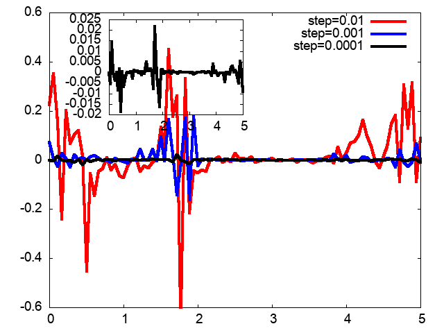
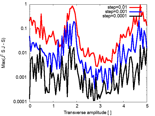
Figure 9: Symplecticity tests with space charge. Difference ${\mathrm{det}[\bf J}$] - 1 (left) and maximum norm of the matrix ${\bf J}^{T}{\bf S}{\bf J}-{\bf S}$ (right) as functions of the transverse amplitude in units of the rms beam size.

Figure 9 shows the results of symplecticity tests with space charge. The largest deviation $\det{\bf J}-1$ is $0.4$ using a step size of $0.01$, it falls to 0.15 at step size $0.001$ and is an order of magnitude smaller (0.02) at step size $0.0001$. The maximum norm $|{\bf J}^{T}{\bf S}{\bf J}-{\bf S}|$ exhibits a similar behavior and reaches its smallest value at step size $0.0001$. Compared to the cases with octupoles but without space charge in Figure 2, the deviations from symplecticity are at least two orders of magnitude larger. Another difference is that the largest deviations occur at a lower betatron amplitude (about 2$\sigma$) and do not increase with amplitude.

The fact that the deviations from symplecticity in pyORBIT in the presence of space charge are significant is not surprising as it is observed in most PIC codes to date. This state of affairs makes these codes not suitable for long term tracking.

4 Emittance Growth and Particle Loss

Predictions of emittance growth and particle loss are two of the many reasons for using a space charge code. We first discuss the results of emittance growth without space charge to estimate the background growth and then at low and full bunch intensity to observe the impact of increasing space charge effects. The top row in Fig. 10 shows the emittance in all three planes without space charge and at a low bunch charge of 10⁶ protons, five orders of magnitude lower than the full intensity. There is no particle loss in either case.

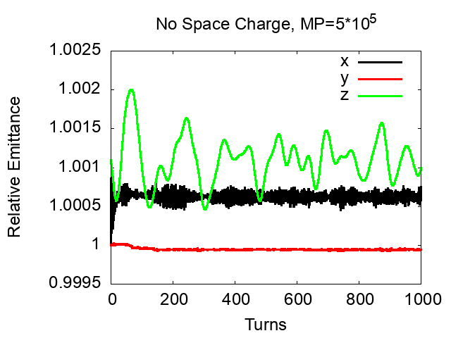
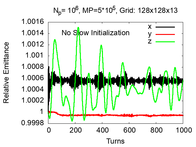
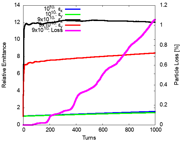
Figure 10: Top: Emittance growth in each plane without space charge (left) and at a low bunch intensity of $10^{6}$ (right). Bottom: Emittance growth (left vertical scale) at intensities 10¹⁰ and $9\times 10^{10}$ and the particle loss (right vertical scale) at the higher intensity. There is no loss at 10¹⁰ over this time scale, hence is not shown.

The influence of dispersion and momentum spread is visible in the transverse emittance. The oscillations in both the horizontal and longitudinal emittance have the same period. The background noise in the transverse emittances is less than 0.1 %. The bottom plot in this figure shows the emittance growth at bunch intensities 10¹⁰ and $9\times 10^{10}$. At the lower intensity, the emittance grows by 20% and there is no loss. At the higher intensity, the emittance growth is dramatic, up to 12 times ($\epsilon_{x}$) and 7 times ($\epsilon_{y}$). The growth occurs over the first few turns and quickly reaches a plateau. The predicted total loss over 1000 turns is $\sim 1\%$, which is unacceptably high for such a short time scale.

4.1 Initial rms matching

As seen in Fig. 10, the mismatch between the bare lattice functions and those with space charge leads to a rapid initial emittance growth and particle loss at full intensity. Properly matching a lattice to space charge induced changes requires matching the Twiss functions so that the beam envelopes have the space charge equilibrium values all around the ring. One way of extracting the matched Twiss functions is to solve the envelope equations for the stationary rms sizes and use the initial emittances to find these matched functions. Instead here we track the unmatched macroparticle distribution for 1000 turns. At the end of this period, we extract the statistical Twiss functions e.g in the horizontal plane as (here $\delta=\Delta p/p$)

$$\langle\beta_{x}\rangle = \frac{\langle x^{2}\rangle}{\sqrt{\langle x^{2}\rangle\langle(x^{\prime})^{2}\rangle-\langle(xx^{\prime})^{2}\rangle}},\;\;\;\langle\alpha_{x}\rangle=-\frac{\langle xx^{\prime}\rangle}{\sqrt{\langle x^{2}\rangle\langle(x^{\prime})^{2}\rangle-\langle(xx^{\prime})^{2}\rangle}}$$ (4.1)

$$\langle D_{x}\rangle = \frac{\langle x\delta\rangle}{\langle\delta^{2}\rangle},\;\;\;\;\langle D_{x}^{\prime}\rangle=\frac{\langle x^{\prime}\delta\rangle}{\langle\delta^{2}\rangle}$$ (4.2)

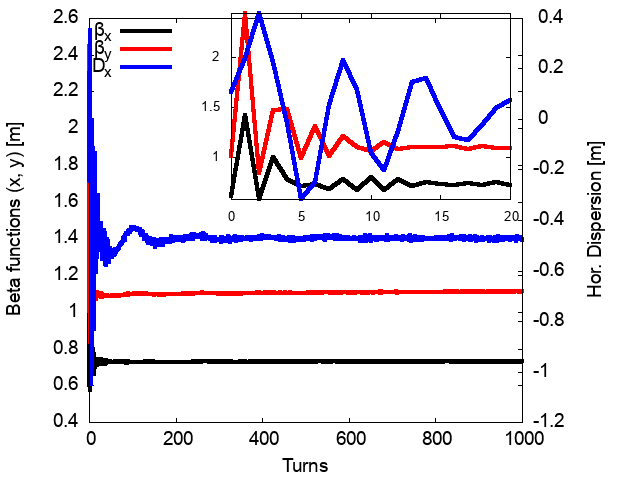
Figure 11: The statistical beta functions (on the left vertical scale) and dispersion (right vertical scale) over time. The inset shows that the beta functions relax to their equilibrium values within 20 turns, the dispersion relaxes over about 200 turns.

Figure 11 shows the evolution of the beta functions. There are sharp transients as the beam adjusts to the space charge forces but the beta functions reach stable values which turn out to be close to their initial values within 20 turns; the same time scale as for the emittance as seen in Fig. 10. The initial beta functions are $(\beta_{x},\beta_{y})=(0.79,1.16)$m and the final values after 1000 turns are (0.73, 1.11)m. The dispersion function relaxes over a longer time scale and changes more significantly from -0.24m to -0.43m. The lattice is then re matched with these values at the initial point in the lattice and is used in the subsequent tracking calculations discussed below.

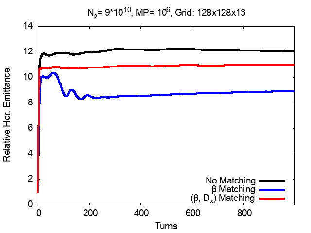
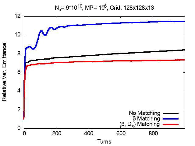
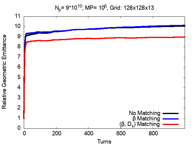
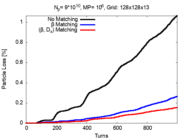
Figure 12: Top row: Relative emittance growth in the horizontal (left) and vertical planes (right) with and without rms matching. Bottom row: The left plot shows the growth of the geometric mean emittance $\sqrt{\epsilon_{x}\epsilon_{y}}$, the right plot shows the particle loss.

Fig. 12 shows the relative emittance and particle loss without matching and rms matching just the $(\beta,\alpha)$ functions and also including the matching the horizontal dispersion $D_{x}$. We observe that the $\epsilon_{x}$ decreases and $\epsilon_{y}$ increases with only beta matching relative to the values without matching. Both these emittances decrease when we add $D_{x}$ matching. The left plot in the bottom row shows that there is no change in the geometric mean emittance $\sqrt{\epsilon_{x}\epsilon_{y}}$ with only beta matching while it drops slightly with additional $D_{x}$ matching. The right plot in the bottom row shows, however, that just beta matching alone reduces the loss by about a factor of five and it drops another factor of two with the addition of matching $D_{x}$. These results show that this rms matching does not significantly affect the emittance growth nor does it slow the time scale of the initial increase.

4.2 Slow Initialization

In this section we describe an alternative procedure to numerically reach a steady state. Rather than injecting with the full charge, the charge per macroparticle is increased linearly from zero to its full value at turn $T_{init}$, the initialization time. Provided this process is sufficiently adiabatic, one expects the beam to remain in near equilibrium at every step as the beam has time to adjust to a slowly changing space charge force.

We note that in this procedure, the number of macro-particles stays constant while the charge per macro-particle increases with time. This is easy to implement in a simulation since all the macro-particles are drawn from an initial distribution; however, the procedure does not mimic the way bunch intensity increases in a real accelerator while the machine is being filled. There are a number of methods available that would allow to more realistically populate each bunch; the details of the subsequent dynamics will be influenced by the chosen method. Such an investigation is left for a future study.

The IOTA beam pipe radius is 25 mm; this value is used as the limiting aperture for simulation purposes. In the actual machine, the available aperture in the nonlinear elements such as the octupoles or the nonlinear lens have smaller apertures. These nonlinear elements are not included here. To distinguish halo growth from core emittance growth, we will also discuss the dynamics with a larger aperture e.g. 100 mm.

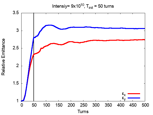
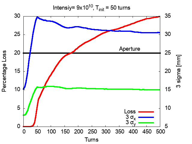
Figure 13: Emittance growth and losses at a slow initialization time of 50 turns and with an aperture of 25 mm.

Figure 13 shows emittance growth and beam loss for two choices of $T_{init}$ with the physical aperture set to 25 mm. Losses start when 3 $\sigma_{x}$ reaches the limiting aperture radius.

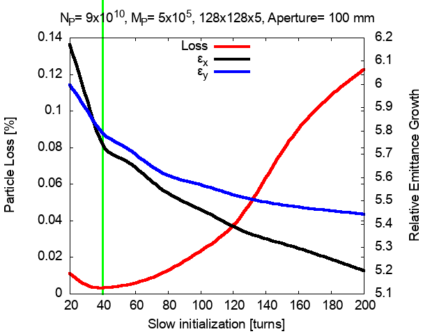
Figure 14: Loss and emittance growth as a function of the slow initialization time.

Figure 14 shows emittance growth and particle loss after 500 turns as a function of the slow initialization time. We observe that the emittance growth decreases monotonically as $T_{init}$ increases and falls by about 15% in the range studied. The losses increase by about 40 fold from the minimum to maximum over this range and are significantly more sensitive to the initialization time. We also observe that there is no reduction in the rms emittances over this range of $T_{init}$, so clearly the core does not reach the aperture. These observations suggest that the halo is strongly affected by the charge on the macroparticles while the growth of the core is less affected. It may be useful to determine why the loss is minimum at 40 turns. We note in passing that the relative emittance change in the transverse planes are nearly equal at this value of $T_{init}$, so that equipartitioning of emittances is apparently correlated with a minimum of losses.

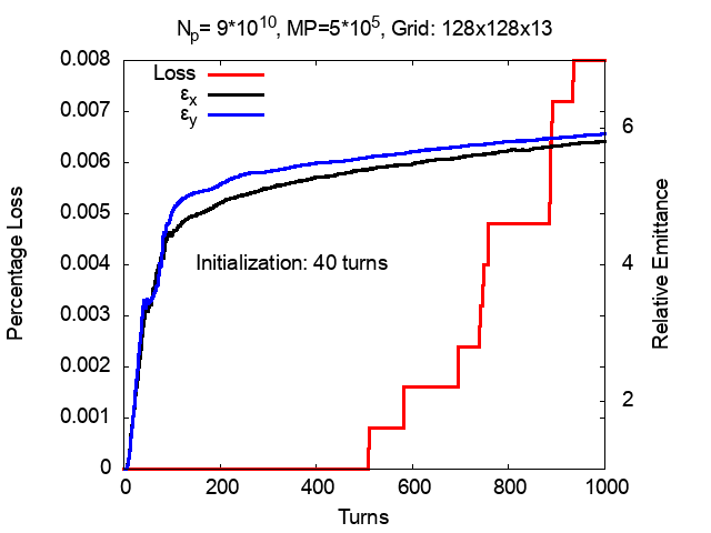
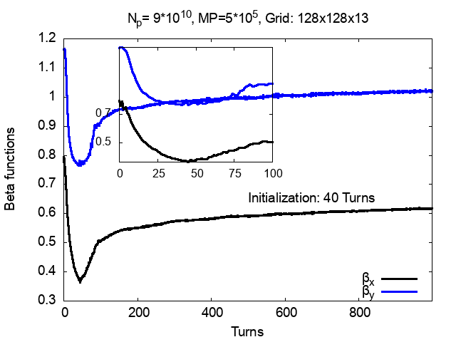
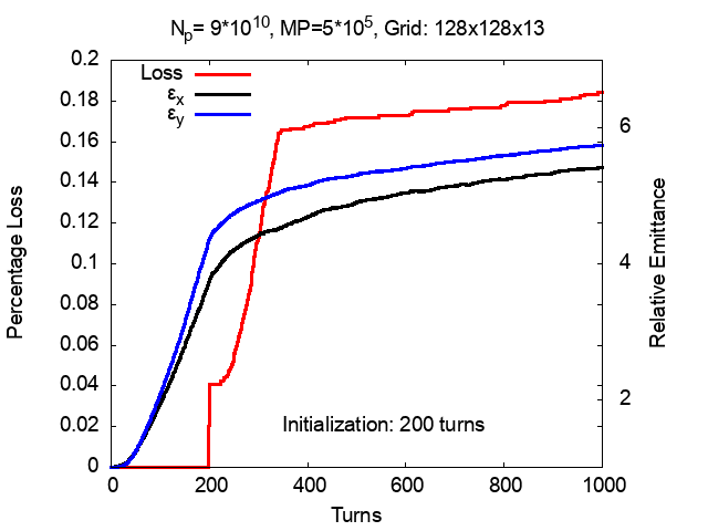
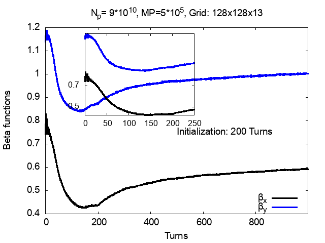
Figure 15: Left: Particle losses (left vertical scale) and relative emittance (right vertical scale), Right: Statistical beta functions for two initialization times : 40 turns (Top) and 200 turns (Bottom).

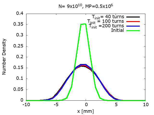
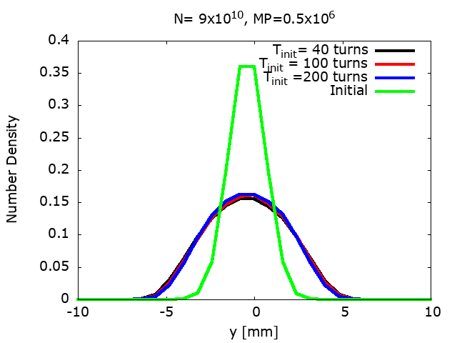
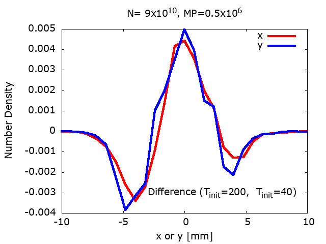
Figure 16: Top: Density profiles for the initialization times that correspond to the smallest and largest losses; horizontal (left) and vertical (right). Bottom: difference in the profiles.

The two left plots in Fig. 15 show the evolution of the emittance growth and particle loss for two initialization times $T_{int}=40,200$ turns. In both cases, the vertical emittance grows slightly more than the horizontal emittance but the change is about the same for both 40 and 200 turn initializations. The horizontal emittance growth is slightly less at $T_{init}=200$ turns. The losses are significantly smaller at 40 turns. The right plots in this figure shows the statistical beta functions for the same two initializations. The inset plots show that both $\langle\beta_{x}\rangle,\langle\beta_{y}\rangle$ reach different stable values depend on $T_{init}$ and that the time to stabilize increases with $T_{init}$. The top plots in Fig. 16 shows the initial and final horizontal and vertical profiles while the bottom plot shows the difference profiles between the two initializations in both planes. These plots show that after stabilization, the profiles do not change much with the initialization time.

4.3 Convergence Tests on simulation parameters

There are three parameters in the pyORBIT simulations that need to be tested for convergence : the number of macroparticles ($M_{P}$), the number of space charge kicks per betatron wavelength ($N_{sc}$) and the number of spatial grid points ($N_{x}\times N_{y}\times N_{z}$) used while solving Poisson’s equation. Increasing $M_{P}$ reduces the statistical noise and a larger $N_{sc}$ ensures better sampling of the spatially dependent space charge kick as the transverse beam sizes vary along the ring. These two parameters have practical upper limits set by the computing time required. Increasing the number of grid points improves the resolution of the sampling of the space charge force. An insufficient number of grid points increase the numerical noise with a PIC code and can lead to artificial emittance growth. Similarly, due to round-off error accumulation, an excessive grid size can lead to the same problem. There is therefore an optimum sampling that provides low enough noise [7] for reasonable computational cost. The number of grid points in each plane is distributed from $-3\sigma_{u}$ to $3\sigma_{u}$, $u=x,y,z$ for Gaussian distributions in these planes, although about 1% of the macro-particles may be at larger amplitudes.

We describe tests performed to determine parameters that ensure convergence by examining the behavior of beam losses and emittance growth. The convergence tests are performed at full intensity ($9\times 10^{10}$) and we use the slow initialization procedure described above with $T_{init}=40$ turns.

pyORBIT assigns at least one space charge kick to each element so there are at least a hundred space charge kicks around the IOTA ring. The exact number of space charge kicks per element is determined by the ratio $L/\Delta s$ where $L$ is the element length and $\Delta s$ is a step length input parameter. Summing over the elements and dividing by the integer part of the tune, $\sim 5$ in IOTA yields the number of space charge kicks per betatron period, $N_{SC}$. For example, $\Delta s=0.1$m yields $N_{SC}=119$ while at a lower resolution choosing $\Delta s=0.4$m yields $N_{SC}$ = 56.

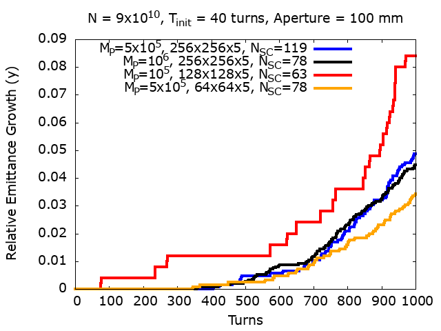
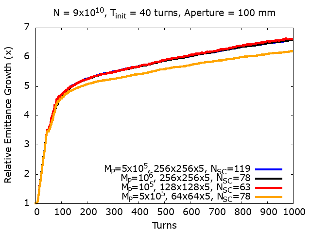
Figure 17: Particle losses (left) and horizontal emittance growth (right) for different combinations of macro-particle numbers, grid sizes and number of space charge kicks. The vertical emittance has the same dependence as the horizontal emittance on these parameters.

Figure 17 shows the particle loss and emittance growth for different numbers of macro-particles, grid sizes and space charge kicks. Other parameters that are held constant are shown at the top of each plot. We observe that losses are generally more sensitive to changes in parameters than the emittance. The losses plot shows that $10^{5}$ macro-particles and a grid size of $64\times 64\times 5$ insufficient. The emittance plot shows that $10^{5}$ macro-particles suffices while a $64\times 64\times 5$ grid yields a lower emittance than finer grids.

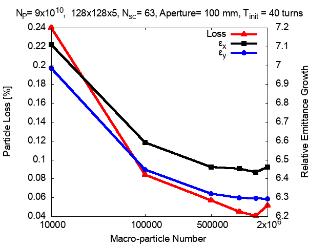
Figure 18: Particle loss (red; left vertical scale) , relative emittance growth (black, blue; right vertical scale) after 1000 turns as a function of the macro-particle number varying over three orders of magnitude,shown on a log scale. The constant parameters are shown at the top.

Fig. 18 shows the dependence of particle loss and emittance growth on the macro-particle number $M_{P}$ with the number of grid points fixed at $128\times 128\times 5$ and number of space charge kicks $N_{sc}$ per betatron wavelength fixed at $63$. Over the range $10^{3}\leq M_{P}<5\times 10^{5}$, the loss is reduced by about a factor of four while at larger values of $M_{P}\geq 5\times 10^{5}$ the loss changes by less than 0.05%. The emittance stays nearly constant over this latter range from which we conclude that $M_{P}=5\times 10^{5}$ is the minimum number of macro-particles required.

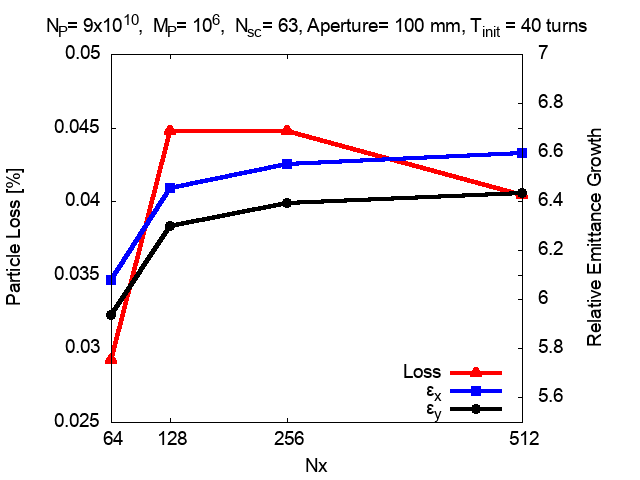
Figure 19: Particle loss (red) , relative emittance growth (black, blue) after 1000 turns as a function of the grid parameter $Nx=Ny$, $Nz=5$. The constant parameters are shown at the top.

Fig. 19 shows the variation of the loss and emittance growth with the number of grid points $N_{x}=N_{y}$ with the number of macro-particles fixed at 10⁶ and $N_{sc}$ fixed at $78$. The emittance stays nearly constant for $128\leq N_{x}\leq 512$ and the loss fluctuates by less than 0.005% over this range. This shows that 128 is the minimum number of grid points required.

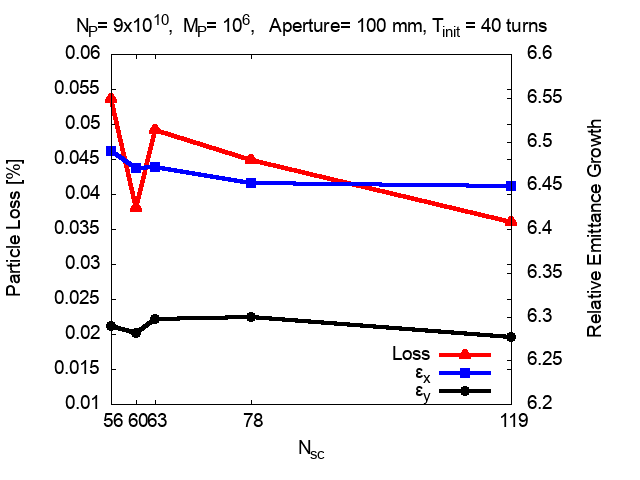
Figure 20: Particle loss (red) , relative emittance growth (black, blue) after 1000 turns as a function of the number of space charge kicks $N_{SC}$ per betatron period The constant parameters are shown at the top. The values of $N_{SC}$ correspond to the step length parameter $\Delta s=0.1,0.2,0.3,0.4$m discussed in the text.

Fig. 20 shows the convergence with respect to $N_{SC}$ with the macro-particle number $M_{P}=10^{6}$ and grid size 128x128x5 held constant. We observe that the loss fluctuates by $\sim 0.015$% while the emittances are nearly constant with $N_{SC}\geq 63$.

5 Small amplitude tune shifts and tune footprints

The goal of this exercise is to validate the accuracy of pyORBIT’s space charge model by comparing the tune shift obtained by tracking to analytical predictions. As mentioned earlier, the only nonlinearity in the lattice model arises from space charge.

It has been pointed out [9] that chaotic motion is observed for small amplitude particles in PIC codes due to numerical noise. One can expect that the effects of this chaos to mostly disappear when ensemble averaging over many particles to calculate statistical variables such as emittances, beam sizes etc. There are likely few analytical estimates of emittance growth with nonlinear space charge.

Keeping in mind the above caveat for tunes at small amplitudes, tune shifts as a function of amplitude due to space charge can nevertheless be compared to analytical results for a Gaussian distribution.

The analytical small amplitude tune shift for a transverse Gaussian distribution is:

$$\Delta Q_{0,sc}=\frac{r_{p}}{\beta_{k}\gamma^{2}\epsilon_{N}}\bar{\lambda}_{L}N_{p}R$$ (5.1)

where $r_{p}$ is the classical proton radius, $\beta$ and $\gamma$ are Lorentz factors, $R$ the effective machine radius, $\epsilon_{N}$ the normalized transverse emittance, $N_{p}$ the number of protons per bunch, and $\bar{\lambda}_{L}$, the effective line density. In all tests, the reference particle at $(z=0,dE=0)$ does not move.

The exact position dependent line density $\lambda(z)$ for a longitudinal water-bag distribution and the average effective line density $\bar{\lambda}_{L}$ are given by [8]

$$\lambda(z) = \frac{1}{C_{wb}}\sqrt{\cos(k_{rf}z)-\cos(k_{rf}z_{max})}$$ (5.2)

$$\bar{\lambda}_{L} = \frac{1}{2C_{wb}}\sqrt{1-\cos(k_{rf}z_{max})}$$ (5.3)

$$C_{wb} = \frac{4}{k_{rf}}\sqrt{1-\cos(k_{rf}z_{max})}E\left(\frac{1}{2}k_{rf}z_{max}|\csc^{2}(\frac{1}{2}k_{rf}z_{max}\right)$$ (5.4)

Here $k_{rf}$ is the rf wave-number $z_{max}$ is half the total bunch length and $E$ is the complete elliptic integral of the second kind. In the limit of short bunches where $k_{rf}z_{max}\ll 1$ the water-bag distribution reduces to the elliptic distribution with a normalized density

$$\lambda(z)=\frac{2}{\pi z_{max}}\sqrt{1-(\frac{z}{z_{max}})^{2}}$$ (5.5)

The IOTA bunch is long and fills the bucket, so the elliptic distribution is not a good approximation.

For the water-bag distribution with $z_{max}=4.5$ meters, the effective line density $\bar{\lambda}_{L}=0.083$. Plugging in all known parameters, and accounting for the fact that $\epsilon_{N}$ changes during tracking we calculate the small amplitude tune shift:

$$\Delta Q_{0,sc}=\frac{-1.09*10^{-17}*N_{p}}{\langle\epsilon_{N}\rangle}$$ (5.6)

where $\langle\epsilon_{N}\rangle$ denotes a suitably time-averaged emittance. We find that the transverse tune shift does not depend very sensitively on the longitudinal distribution. Figure 21 shows the absolute value of the space charge tune shift as a function of the maximum longitudinal extent $z_{max}$ of a bunch for different distributions. At $N_{b}=9\times 10^{0}$ and $z_{max}=4.5$m, the tune shifts are $\Delta Q_{sc,0}=(-0.554,-0.521,-0.514)$ for the Gaussian, parabolic and water-bag distributions respectively.

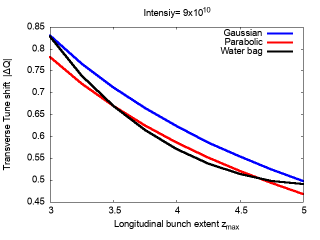
Figure 21: Absolute transverse tune shift as a function of the longitudinal extent $z_{max}$ for different distributions.

5.1 Small Amplitude Tune Shift

We calculate the transverse tunes using two different methods. First we use the definition of the tune as the number of transverse oscillations in one revolution to calculate the small amplitude tune. The bunch is initialized as shown in Figure 8. It is tracked for 500 turns and the first 200 turns are used for slow initialization. At this point, a test particle is added at a nearly zero amplitude ($0.01\sigma_{x}$, 0, $0.01\sigma_{y}$, 0, 0, 0). The bunch is tracked for an additional 1000 turns, during which all monitors in the IOTA lattice record the transverse position of the test particle at every turn. Counting the total number of zero crossings and dividing by twice the number of turns monitored yields a lower bound for the small amplitude tune.

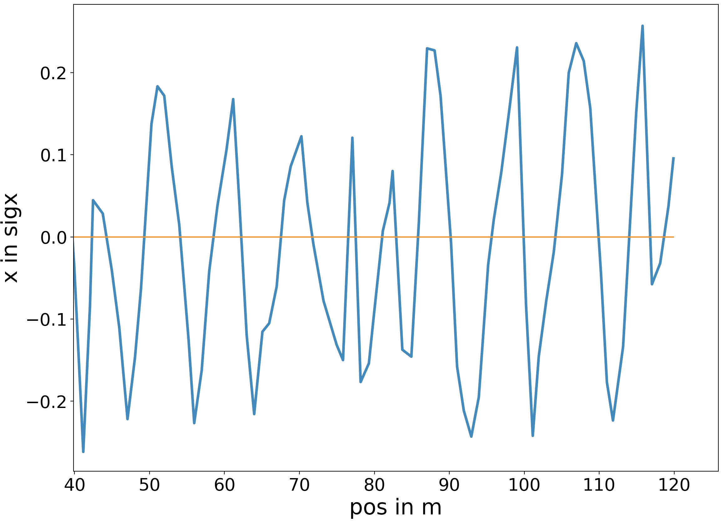
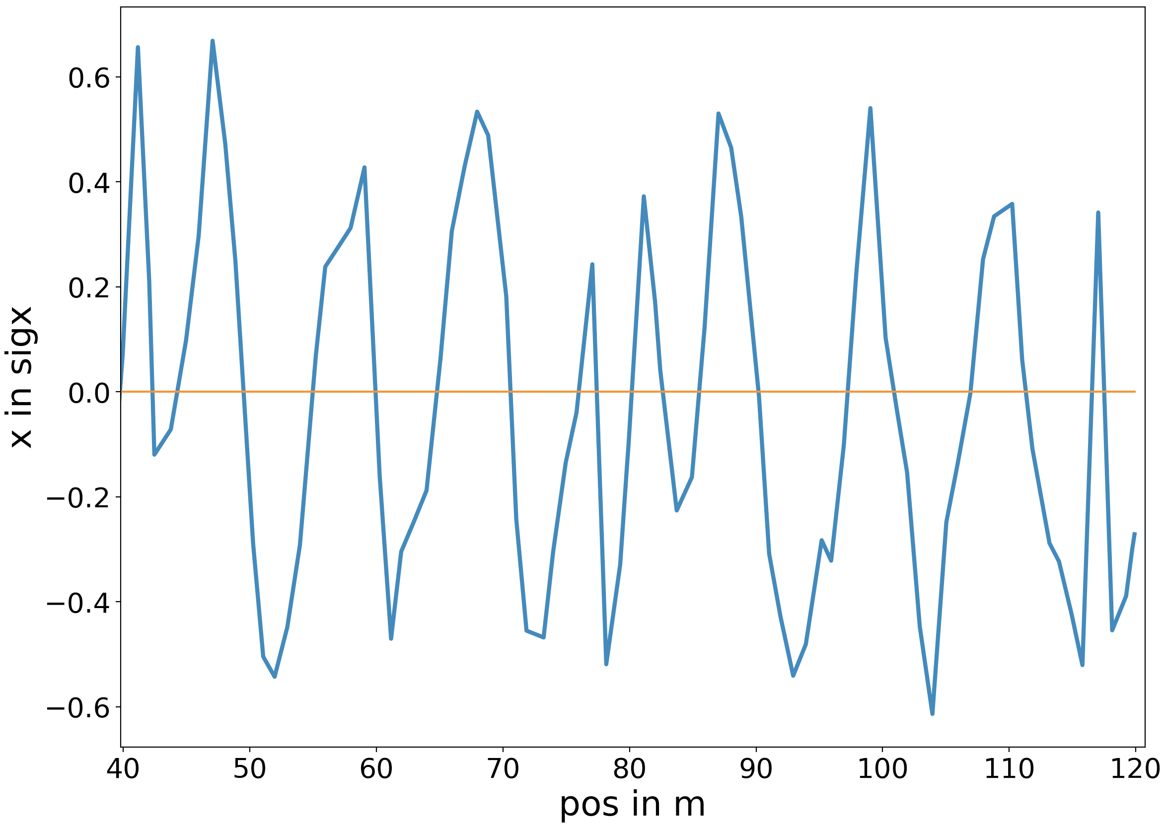
Figure 22: Betatron oscillations over two turns : (a) Zero intensity (left), 21 zero crossings (b) Bunch charge $9\times 10^{10}$ (right), 19 zero crossings.

Fig. 22 shows the betatron oscillations over two turns for two bunch intensities. The number of zero crossings allows us to extract the tune with a precision of 0.25 over the following ranges: (a) Zero and $10^{9}$ intensities: $5.25<Q_{x}<5.5$, (b) $10^{10}$ intensity: $5.0<Q_{x}<5.25$ and (c) $10^{10}$ intensity: $4.75<Q_{x}<5.0$. Table 3 shows the tunes calculated from betatron oscillations with higher precision using 1000 turns and the fractional tunes calculated with an FFT using the same number of turns. The FFT tune is averaged over 100 particles placed at the same small amplitude in an effort to reduce the fluctuations due to chaotic motion reported in [9].

Intensity	Small amplitude tunes $Q_{x},Q_{y}$
	Betatron Oscillations	FFT
0	(5.300, 5.301)	(0.2988, 0.3)
$10^{9}$	(5.2681, 5.267)	(0.2663, 0.265)
$10^{10}$	(5.037, 5.023)	(0.039, 0.035)
$9\times 10^{10}$	(4.873, 4.973)	(0.951, 0.975)
Intensity	Small amplitude tune shifts
	Theory	Simulation
0	(0.0, 0.0)	(0.0, 0.001)
109	(-0.037, -0.037)	(-0.03, -0.034)
1010	(-0.29, -0.29)	(-0.262, -0.266)
9$\times 10^{10}$	(-0.514 -0.514)	(-0.50, -0.536)

Table 3: Small amplitude tunes from betatron oscillations and the fractional tunes from an FFT, in both cases using 1000 turns of data. Also shown are the small amplitude transverse tune shifts calculated from theory and simulations at different intensities.

5.2 Tune Footprints

The amplitude-dependent tunes for a transverse Gaussian distribution can be calculated analogously to those from a head-on beam-beam interaction between two Gaussian beams. For a round beam, the tunes are [8]

$$\Delta Q_{x,sc} = \Delta Q_{0,sc}\int_{0}^{\infty}\exp[-(\alpha_{x}+\alpha_{y})u]I_{0}(\alpha_{y}u)\left[I_{0}(\alpha_{x}u)-I_{1}(\alpha_{x}u)\right]du$$ (5.7)

$$\Delta Q_{y,sc} = \Delta Q_{0,sc}\int_{0}^{\infty}\exp[-(\alpha_{x}+\alpha_{y})u]I_{0}(\alpha_{x}u)\left[I_{0}(\alpha_{y}u)-I_{1}(\alpha_{y}u)\right]du$$ (5.8)

$$\alpha_{x} = \frac{a_{x}^{2}}{4},\;\;\;\;\alpha_{y}=\frac{a_{y}^{2}}{4},\;\;\;a_{x}=\frac{x}{\sigma_{x}},\;a_{x}=\frac{y}{\sigma_{y}}$$ (5.9)

where $a_{x},a_{y}$ are the dimensionless amplitudes. Slightly more complex expressions exist for non-round beams, but those will not be used here.

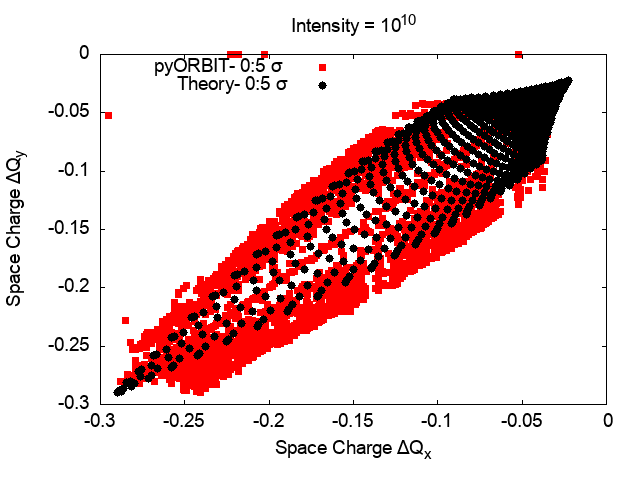
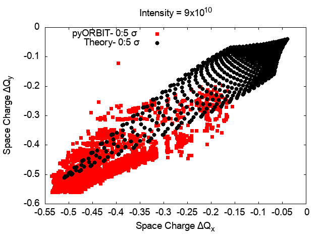
Figure 23: Tune shifts with amplitude due to space charge from pyORBIT and theory at intensity $10^{10}$ (left) intensity $9\times 10^{10}$ (right). In both cases, the pyORBIT simulation ranges from 0-5$\sigma$ (due to aperture limitations) and the theoretical footprint using Eqs.(5.7) and (5.8) extends to 5$\sigma$.

The tune footprints are calculated with a bunch initially tracked for 1000 turns (including 40 turns of slow initialization, as described in Section 4.2) to allow emittance to stabilize and get closer to an equilibrium value. After this initial period, 5000 test particles are injected with initial conditions distributed along semi-circular arcs on radii from (0-5)$\sigma$ in $x-y$ space; particles initially at larger amplitudes would be lost at the physical aperture. The bunch and the test particles are tracked for another 1000 turns to obtain the fractional tunes using an FFT. At intensity $N_{b}=9\times 10^{10}$, the lattice tune is shifted to $Q_{x}=5.46$ and $Q_{y}=5.44$ to avoid the presence of resonances (possibly “stochastic resonances”) within the footprint. The tune footprints in Figure 23 show both theoretical and pyORBIT simulation results. The theoretical footprint also extends to 5$\sigma$. At intensities at below 10¹⁰ and below, the simulated footprint matches the theoretical footprint quite well but is wider. At 9$\times 10^{10}$, the asymmetry between $\Delta Q_{x,sc},\Delta Q_{y,sc}$ in the simulated tunes increases with $\mid\Delta Q_{x,sc}\mid<\mid\Delta Q_{y,sc}\mid$, possibly due to the dispersion contribution to the horizontal beam size. Simulations of the emittance growth (discussed in Section 4) show that the final emittance is about 6.4 times larger than the initial emittance; this was the value assumed for $\epsilon_{N}$ in the theoretical footprint. The small amplitude tuneshift in Table 3 shows that the difference between the average of the simulated tune shifts $(\Delta Q_{x,sc}+\Delta Q_{y,sc})/2$ and the theoretical value is 0.004, a few times 0.001, the precision of the FFT calculation; however, the simulated footprint is significantly wider (by about 0.05 in tune units) than the theoretical footprint. At large amplitudes close to 5$\sigma$, the simulated tune shifts are larger than expected from theory. Some differences are to be expected since the theoretical model assumes a zero length bunch, so does not include the longitudinal dependence of the transverse space charge force. Nor does the theory include the effect of dispersion but this can be done easily, if required. Finally there is numerical noise in the PIC code which will impact the tune footprint which is calculated without averaging.

6 Conclusions

• The symplectic nature of single particle tracking with pyORBIT was checked for both the linear lattice and the lattice with octupoles using two measures: $(\det\mathsf{J}-1)$ and $\mathrm{max}(\mathsf{J}^{T}\mathsf{S}\mathsf{J}-\mathsf{S})$. $\mathsf{J}$ is the Jacobian matrix of the transfer map and $\mathsf{S}$ is the symplectic matrix. On both measures, the pyORBIT model’s deviation from symplecticity is $\sim 10^{-11}$ for the linear lattice. This deviation increases to $\sim 10^{-4}$ with the octupoles. By comparison, the same tests using MADX show the same measures to be $\sim 10^{-8}$ for the linear lattice and $\sim 10^{-4}$ with octupoles.

  The variance of the Hamiltonian is similar with both codes.

  The transverse tunes calculated with octupoles in the lattice agree to within 10^-3 over the stable region of phase space. The boundary where the differences are about an order of magnitude larger is close to the dynamic aperture; the tune difference map resembles an FMA map produced by a single code. The dynamic apertures found by the two codes agree remarkably to within 1% with or without synchrotron oscillations (see Table 2 ).

• The main purpose of using pyORBIT is for its space charge tracking which is based on a PIC style method. Such codes are not symplectic and indeed find that the deviations from symplecticity are about two orders of magnitude larger than in the single particle version with octupoles. This shows that the space charge tracking results cannot be used with confidence for long-term tracking. However we expect that short term results ($\sim 10^{3}-10^{4}$ turns) should be reliable for parametric studies.

• The IOTA lattice we have used for the space charge studies is the original linear lattice. This lattice is not rms matched to the space charge lattice functions and the mismatch increases with the bunch intensity. At full intensity, this mismatch leads to almost ten-fold increase in transverse emittance and the beam loss is about 1% after 1000 turns. Most of the emittance increase occurs over the first few turns due to a large mismatch. In order to reduce the emittance growth and loss in this mismatched lattice, first we matched the lattice for a Gaussian distribution with initial rms sizes the same as the final values. This reduced the emittance growth slightly but lowered the losses to 0.1% over 1000 turns. Next we introduced a slow initialization time $T_{init}$ (without rms matching) during which the charge on each macro-particle is increased linearly over time. We find that this reduces both the emittance growth to about five-fold and especially the losses to less than 0.1% over the same time. The optimum initialization time $T_{init}$ is found to be 40 turns for which the loss is about 0.01%.

• With the optimum slow initialization time fixed at 40 turns, we tested for convergence by examining the behavior of the emittance growth and the particle loss as one of three important parameters was varied while keeping the other two parameters fixed. In general, the loss shows more fluctuations than the emittance as the parameters are varied. However with the aperture set at 100 mm (to avoid an emittance reduction due to significant losses), the losses are typically around 0.05% and fluctuations at the 10% level are not significant. Figure 18 shows the minimum number of macro-particles needed is 5$\times 10^{5}$ keeping the grid size fixed at 128x128x5 and the number of space charge kicks per betatron wavelength $N_{sc}=63$. Figure 19 shows that the emittance growth stabilizes at the grid size 128x128x5 and does not change much upto grid sizes 512x512x5. Finally 20 shows that convergence is achieved with $N_{sc}=78$ but $N_{sc}=63$ can be used without significant differences. This value of $N_{sc}$ is quite a bit larger than typically expected.

• The space charge small amplitude tune shifts and tune footprints agree quite well with theoretical predictions up to a bunch intensity of $10^{10}$. At the maximum intensity of $9\times 10^{10}$, the small amplitude tune shifts still agree reasonably but the simulated footprint is somewhat wider than the theoretical footprint (see Fig 23b). In making the comparison, we have to take into account the emittance growth at full intensity.

To sum up, we have established that pyORBIT matches MADX very closely for single particle tracking. The space charge model of pyORBIT is not designed to be symplectic, so naturally the deviations from symplecticity are significant. Nevertheless, we find that the space charge tuneshifts calculated over 1000 turns with pyORBIT agree reasonably well with theory. We believe therefore that over the time scale of 10³- 10⁴ turns, pyORBIT can be used with confidence. This report dealt only with the transverse space charge effects, so similar issues will be need to be examined when the longitudinal space charge effects are included.

Acknowledgments
We thank the Lee Teng internship program at Fermilab which enabled the participation of Runze Li in this study. Fermilab is operated by Fermi Research Alliance LLC under DOE contract No. DE-AC02CH11359.

A Appendix: Beam temperature and chromaticity

The transverse temperature is

$$T_{\perp}=\gamma m_{0}\langle v_{\perp}^{2}\rangle$$ (A.1)

The mean squared transverse velocities can be found from

$$v_{\perp} = \frac{p_{\perp}}{m_{0}}=\frac{p_{0}}{m_{0}}u^{\prime},\;\;\;\;u=x,y$$

$$\langle v_{x}^{2}\rangle = (\frac{p_{0}}{m_{0}})^{2}\langle(x^{\prime})^{2}\rangle=(\frac{p_{0}}{m_{0}})^{2}\gamma_{x}\epsilon_{x}$$

$$= \frac{1}{(m_{0}c)^{2}}[E^{2}-(m_{0}c^{2})^{2}]\gamma_{x}\epsilon_{x}=c^{2}[\gamma^{2}-1]\gamma_{x}\epsilon_{x}$$

The above average represents an average over the beam distribution.

Averaging over the ring, we have

$$\langle k_{B}T_{\perp}\rangle=m_{0}c^{2}[\gamma^{2}-1]\epsilon_{x,N}<\gamma_{x}>$$ (A.2)

To find the ring average of $\gamma_{x}$, we use [10]

$$K_{x}\beta_{x} = \alpha_{x}^{\prime}+\gamma_{x}$$ (A.3)

$$\Rightarrow-4\pi Q_{x}^{\prime} = \oint(\alpha_{x}^{\prime}+\gamma_{x})ds=\oint\gamma_{x}ds=C\langle\gamma_{x}\rangle$$ (A.4)

where $K_{x}$ is the quadrupole gradient parameter, $Q_{x}^{\prime}$ is the natural chromaticity and $C$ is the machine circumference. Hence

$$\langle\sigma_{x^{\prime}}^{2}\rangle=\langle\gamma_{x}\rangle\epsilon_{x}=-\frac{2Q_{x}^{\prime}}{R}\epsilon_{x}$$ (A.5)

where $R$ is the machine radius. We recall that the average rms size is given approximately by

$$\langle\sigma_{x}^{2}\rangle=\langle\beta_{x}\rangle\epsilon_{x}=\frac{R}{Q_{x}}\epsilon_{x}$$ (A.6)

We note that while Eq. (A.6) for the rms size requires the smooth focusing approximation wherein $\langle 1/\beta_{x}\rangle\approx 1/\langle\beta_{x}\rangle$, Eq. (A.5) for the divergence does not require any approximation and remains valid even with nonlinear magnets in the ring. From these two equations we observe that the average beam size and divergence are determined by the tune and natural chromaticity respectively.

The average temperature over the ring is therefore

$$\langle k_{B}T_{x}\rangle=m_{0}c^{2}(\gamma^{2}-1)[\frac{-2Q_{x}^{\prime}}{R}]\epsilon_{x,N}$$ (A.7)

where $\epsilon_{x,N}$ is the normalized emittance.

B Appendix: Additions and changes to pyORBIT

This appendix describes additions and modifications to the original pyORBIT program[1], including a new dipole edge element and the optional elimination of nonlinearities in the dipole and quadrupole elements. A number of bugs found in pyORBIT have been corrected. All additions and modifications are included in our repository on github [1].

B.1 Adding Dipole Edge Element in pyORBIT

In the original version of pyORBIT, there is no distinct dipole edge element. In order to add dipole edge corrections to pyORBIT, changes were made in three sections of the code: the parser, the tracking method and the python element wrapper.

In the parser, found in the source file py-orbit/py/orbit/teapot/teapot.py a new dipole edge element class named DipedgeTEAPOT was introduced. When an element of type ”dipedge” is encountered by the pyORBIT MADX sequence parser, a new DipedgeTEAPOT element is instantiated. Its parameters, e1, h, hgap, and fint correspond to the dipole edge parameters in MADX. e1 is the rotation angle for the pole face, h is the curvature $\frac{1}{\rho}$, hgap is the half gap of the (upstream/downstream) bending magnet and fint is the edge field integral. The edge is implemented as a thin element i.e. it has length 0. The DipedgeTEAPOT tracking method invoked by the tracker is defined in the source file py-orbit/src/teapot/teapotbase.cc. The implementation considers only first order terms. The corresponding transfer matrix is[11]:

$$\begin{bmatrix}x\\ x^{\prime}\end{bmatrix} = \begin{bmatrix}1&0\\ h\tan(e)&1\\ \end{bmatrix}\begin{bmatrix}x_{0}\\ x^{\prime}_{0}\end{bmatrix}$$ (B.1)

$$\begin{bmatrix}y\\ y^{\prime}\end{bmatrix} = \begin{bmatrix}1&0\\ -h\tan(e-\psi)&1\\ \end{bmatrix}\begin{bmatrix}y_{0}\\ y^{\prime}_{0}\end{bmatrix}$$ (B.2)

$$\psi = {\tt fint}\cdot 2\cdot{\tt hgap}\cdot h\cdot\frac{1+\sin^{2}(e)}{\cos(e)}$$ (B.3)

where $e$ is either the entrance or the exit edge angle.

A new wrapper method was added to make the edge element and its methods available from python. The implementation can be found in the file
py-orbit/src/teapot/wrap_teapotbase.cc.

pyORBIT now handles the dipole edges in the IOTA lattice MADX sequence. When these edges are accounted for, the bare lattice tune $Q_{y}$ calculated by pyORBIT is 5.3, in agreement with MADX; without them pyORBIT predicts 5.42.

B.2 Nonlinear Effects of Magnet Edge

MADX and pyORBIT use different approaches for tracking. MADX operates converts every element to thin kicks. In contrast pyORBIT treats some elements as thick lenses. These elements are further subdivided; a variable called nparts controls the subdivision. For example, a dipole with nparts = n, is treated as follows by pyORBIT:

Fringe In, Entrance, Dipole_1, ....., Dipole_n-2, Exit, Fringe Out

Fringe In and Fringe Out account for edge effects the other n parts (including entrance and exit) are main body of this dipole element. The length (and bending angle for dipole) is distributed among each of these n parts according to $l_{entrance}=l_{exit}=\frac{l_{others}}{2}=\frac{L}{2*(n-1)}$. The entrance contains only linear transformation and other elements have both linear and nonlinear part. Since every element needs an entrance and an exit, ${\tt nparts}\geq 2$.

When tracking a test particle with initial conditions ($\sigma_{x}$, 0, $\sigma_{y}$, 0, 0, 0) for 5000 turns in both MADX and pyORBIT, the two codes produce very different results.

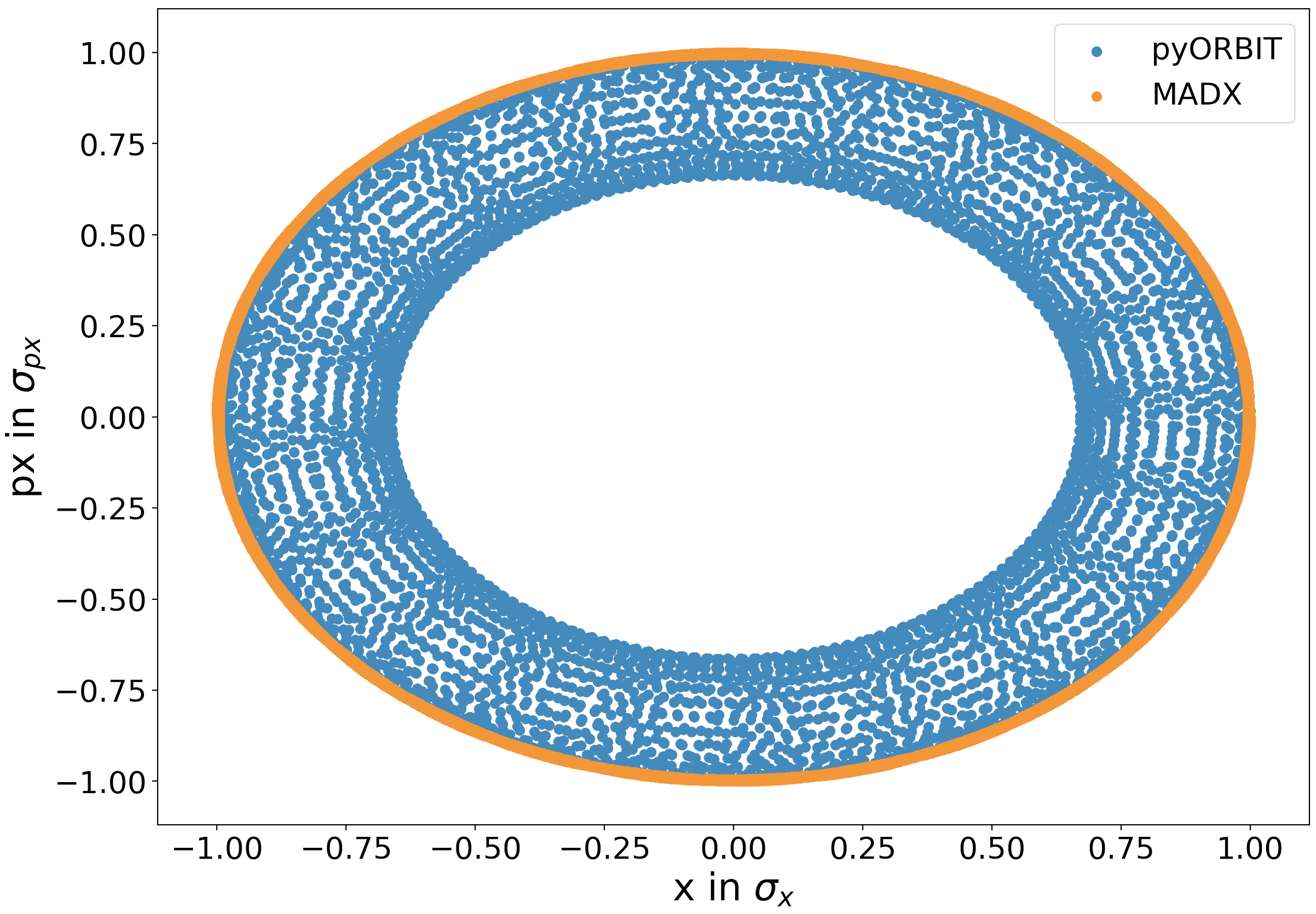
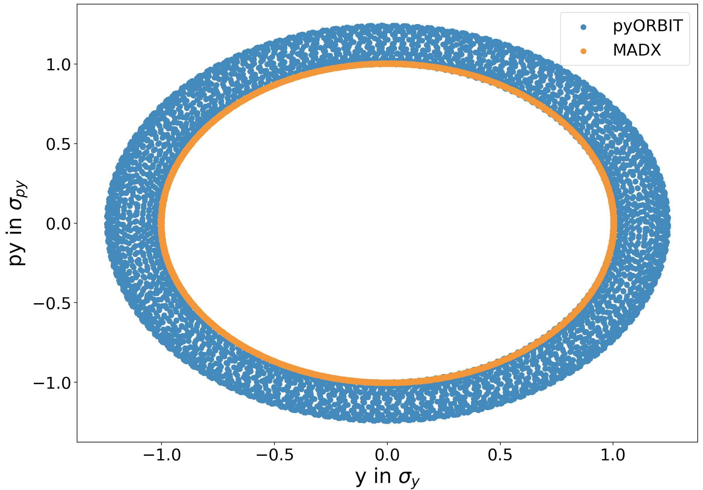
Figure 24: Single particle phase space diagram by MADX and pyORBIT

As shown in figure 24, the trajectories in the $x$-$p_{x}$ and $y$-$p_{y}$ planes show differences on the order of $30\%$. The shape of phase space trajectory produced by pyORBIT suggests the excitation of a resonance by presence of nonlinearities in pyORBIT. After removing all sources of nonlinearity in pyORBIT, we identified the Fringe In and tt Fringe Out sections of the dipole and quadrupole element as the culprit. Their contributions are defined in the file py-orbit/src/teapot/teapotbase.cc.
Removing these methods completely produced the figure 25.

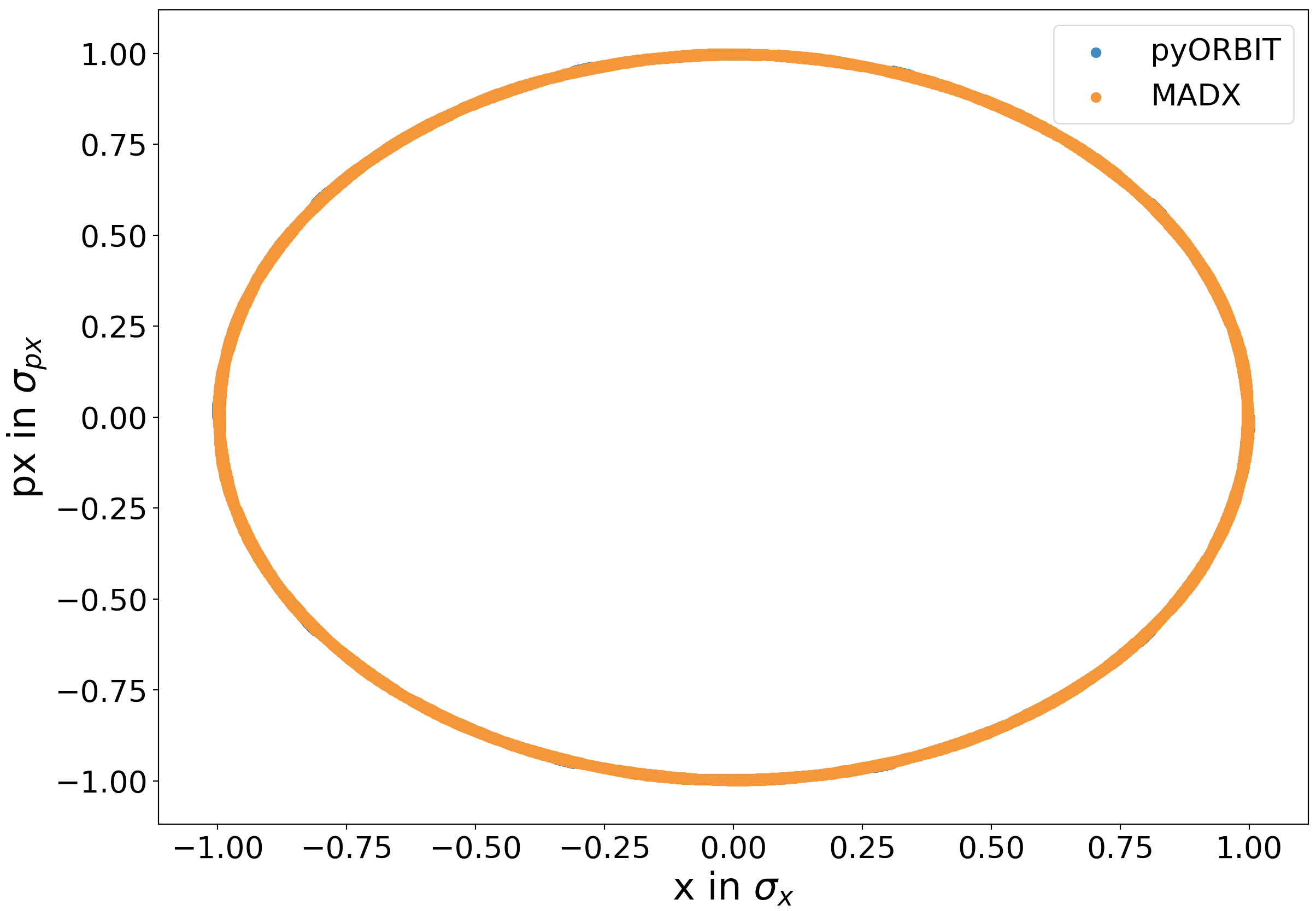
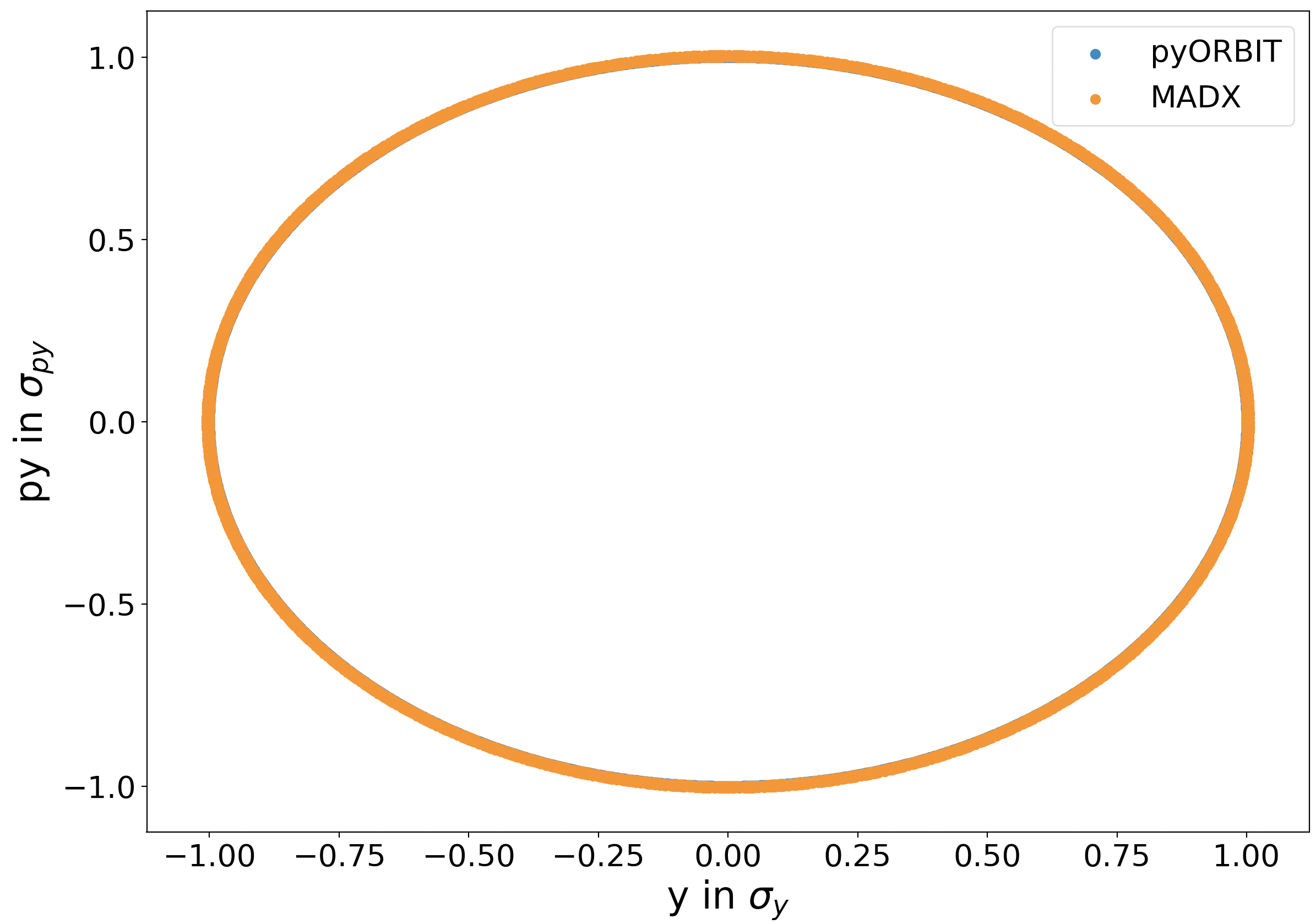
Figure 25: Single particle phase space diagram by MADX and pyORBIT after removing the magnet edge effect

MADX does not consider nonlinear fringe effects; however, for small a ring like IOTA they may be significant. Additional tests would be required to assess the importance of nonlinear edge effects in IOTA.

B.3 Other Changes

A number of bugs in the pyORBIT code were found and corrected. They are listed here.

• In the IOTA sequence generated by MADX, the strength of solenoids is set to the default value 0; this triggered a division by 0 error in pyORBIT. As a workaround, the strength of such solenoids can be manually set to a very small value like $10^{-10}$.

• In the file py-orbit/py/orbit/teapot/teapot.py, the method initialize() of class ApertureTEAPOT initializes the Aperture object with
  Aperture(shape, dim[0], dim[1], 0.0, 0.0),
  however the Aperture object is created by Aperture(int shape, double a, double b, double c, double d, double pos) so a total of 6 parameters are needed. A dummy value 0.0 was added to fix this.

• Also, the treatment of apertures in pyORBIT still has issues with sequence files generated by MADX. The pyORBIT parser looks for elements of type Aperture in the sequence; however, in the IOTA lattice an aperture can be defined using a marker with attribute ”aperture”. The current workaround is to remove all apertures defined in the sequence and add them back later using python code.

• Other bugs fixed in pyORBIT include three methods in the code
  py-orbit/py/orbit/aperture/ApertureLatticeRangeModifications.py,
  which add apertures upstream and downstream of all elements, and one method in the file
  py-orbit/src/orbit/ Aperture/Aperture.cc,
  which checks for particles intercepted at the aperture and moves them to the lostbunch.

References

- [1] https://github.com/PyORBIT-Collaboration/py-orbit
- [2] T. Wangler, Emittance growth from space charge forces, Los Alamos report LA-UR-91-3287
- [3] M. Reiser, Theory and Design of Charged Particle Beams, Wiley, New York
- [4] V. Danilov and S. Nagaitsev, Nonlinear Accelerator Lattices with One and Two Analytic Invariants, Phys. Rev. ST-AB, 13, 084002 (2010)
- [5] S. Antipov et al, IOTA (Integrable Optics Test Accelerator): Facility and Experimental Beam Physics Program, JINST 12, T03002 (2017)
- [6] I. Hoffmann and O. Boine-Frankenheim, Grid dependent noise and entropy growth in anisotropic 3d particle-in-cell simulation of high intensity beams, Phys. Rev. ST-AB, 17, 124201 (2014)
- [7] F. Kesting and G. Franchetti, Propagation of numerical noise in particle-in-cell tracking, Phys. Rev. ST-AB, 18, 114201 (2015)
- [8] T. Sen, unpublished notes
- [9] F. Schmidt et al, Code bench-marking for long-term tracking and adaptive algorithms, Proceedings of HB2016,, p 357 (2016)
- [10] D. Edwards and M.J. Syphers, Section 3.4.3 in An Introduction to The Physics of High Energy Accelerators, Wiley, New York
- [11] Karl L. Brown. A First- and Second-Order Matrix Theory for the Design of Beam Transport Systems and Charged Particle Spectrometers. SLAC Report-75