Intrinsic Superconducting Diode Effect

Abstract

Stimulated by the recent experiment [F. Ando et al., Nature 584, 373 (2020)], we propose an intrinsic mechanism to cause the superconducting diode effect (SDE). SDE refers to the nonreciprocity of the critical current for the metal-superconductor transition. Among various mechanisms for the critical current, the depairing current is known to be intrinsic to each material and has recently been observed in several superconducting systems. We clarify the temperature scaling of the nonreciprocal depairing current near the critical temperature and point out its significant enhancement at low temperatures. It is also found that the nonreciprocal critical current shows sign reversals upon increasing the magnetic field. These behaviors are understood by the nonreciprocity of the Landau critical momentum and the change in the nature of the helical superconductivity. The intrinsic SDE unveils the rich phase diagram and functionalities of noncentrosymmetric superconductors.

Introduction. — Rectification by the semiconductor diode is one of the central building blocks of electronic devices. Apart from the nonreciprocity induced by asymmetric junctions, it has been revealed that nonreciprocal transport can be obtained as a bulk property of materials Tokura and Nagaosa (2018); Ideue and Iwasa (2021). Magnetochiral anisotropy (MCA) Rikken et al. (2001); Krstić et al. (2002); Pop et al. (2014); Rikken and Wyder (2005); Ideue et al. (2017); Wakatsuki and Nagaosa (2018); Hoshino et al. (2018); Wakatsuki et al. (2017); Qin et al. (2017); Yasuda et al. (2019); Itahashi et al. (2020) is an example, described by the equation $R(j)=R_{0}(1+\gamma j{h}).$ Here $R$, $j$, and ${h}$ are the resistance, electric current, and the magnetic field, respectively. The coefficient $\gamma$ gives rise to different resistance for rightward and leftward electric currents and can be finite in noncentrosymmetric materials. MCA has been observed in (semi)conductors Rikken and Wyder (2005); Ideue et al. (2017); Krstić et al. (2002); Pop et al. (2014) as well as in superconductors Wakatsuki et al. (2017); Qin et al. (2017); Yasuda et al. (2019); Itahashi et al. (2020), and allows us to access various aspects of noncentrosymmetric materials: from spin-orbit splitting in the band structure Ideue et al. (2017) to the spin-singlet and -triplet mixing of Cooper pairs Wakatsuki et al. (2017); Wakatsuki and Nagaosa (2018); Hoshino et al. (2018)

MCA is the inequivalence of $R(j)$ and $R(-j)$, where both $R(\pm j)$ usually take finite values. On the other hand, such a drastic situation is possible in superconductors that either one of $R(\pm j)$ vanishes while the other remains finite [Fig. 1]. Such a superconducting diode effect (SDE) has recently been observed in the Nb/V/Ta superlattice without an inversion center and is controlled by the applied inplane magnetic field Ando et al. (2020). This is the first report of the SDE in a bulk material, while similar effects have been recognized in engineered systems Reynoso et al. (2008); Zazunov et al. (2009); Margaris et al. (2010); Yokoyama et al. (2014); Silaev et al. (2014); Campagnano et al. (2015); Dolcini et al. (2015); Chen et al. (2018); Minutillo et al. (2018); Pal and Benjamin (2019); Kopasov et al. (2021) and followed by recent SDE experiments Baumgartner et al. (2021); Lyu et al. (2021). SDE is a promising building block of the dissipationless electric circuits, and is a fascinating phenomenon manifesting the interplay of the inversion breaking and superconductivity. One of the remaining issues is to identify suitable materials providing the best performance; however, the mechanisms to cause SDE in a bulk material Ando et al. (2020) have not been clarified, while the SDE in artificial devices Lyu et al. (2021); Baumgartner et al. (2021) has been well simulated by Bogoliubov-de Gennes (BdG) Baumgartner et al. (2021) and time-dependent Ginzburg-Landau (GL) theories Lyu et al. (2021).

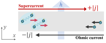
Figure 1: Schematic figure for the SDE. The system has zero and finite resistance for the rightward and leftward current, respectively, and vice versa when the magnetic field $h$ is reversed.

SDE is the nonreciprocity of the critical current for the resistive transition. In usual situations, in particular, under out-of-plane magnetic fields, the resistive transition is caused by the vortex motion. The details of the vortex motion depend on the device setup such as impurity concentrations Blatter et al. (1994), and in turn, has an advantage of tunability by the nanostructure engineering Villegas et al. (2003); Lyu et al. (2021). Apart from the extrinsic mechanisms to cause resistivity, the depairing current is known as the critical current unique to each superconducting material. Here, the metal-superconductor transition is literally caused by the dissociation of the flowing Cooper pairs Tinkham (2004); Dew-Hughes (2001). The depairing current always gives the upper limit of the critical current and is an important material parameter characterizing superconductors Blatter et al. (1994). The depairing limit generally requires a huge current density, but is within the scope of experimental techniques. Indeed, the depairing limit has recently been achieved in the microbridge superconducting devices of YBa₂Cu₃O_7-δ Nawaz et al. (2013), Ba_0.5K_0.5Fe₂As₂ Li et al. (2013), and Fe_1+yTe_1-xSe_x Sun et al. (2020).

In this Letter, as a first step of the theoretical research on SDE of bulk materials, we propose the intrinsic mechanism of SDE by studying the nonreciprocity in the depairing current. The results can be tested with the microbridge experiments and establish the foundation of the future study on the bulk SDE. Furthermore, it is revealed that the intrinsic SDE is closely related to the Flude-Ferrell-Larkin-Ovchinnikov state Larkin and Ovchinnikov (1964); Fulde and Ferrell (1964). While the Larkin-Ovchinnikov (LO) state with the spatially inhomogeneous pair potential $\Delta(x)=\Delta\cos qx$ has been discussed for FeSe Kasahara et al. (2014, 2020), CeCoIn₅ Matsuda and Shimahara (2007) and organic superconductors Wosnitza (2018), the Flude-Fellel (FF) type order parameter $\Delta(x)=\Delta e^{iqx}$ is known to ubiquitously appear in noncentrosymmetric superconductors and is particularly called the helical superconductivity Bauer and Sigrist (2012); Smidman et al. (2017); Agterberg (2003); Barzykin and Gor’kov (2002); Dimitrova and Feigel’man (2003); Kaur et al. (2005); Agterberg and Kaur (2007); Dimitrova and Feigel’man (2007); Samokhin (2008); Yanase and Sigrist (2008); Bauer and Sigrist (2012); Michaeli et al. (2012); Sekihara et al. (2013); Houzet and Meyer (2015). Implications of the helical superconductivity have been obtained in thin films of Pb Sekihara et al. (2013) and doped SrTiO₃ Schumann et al. (2020), and a heavy-fermion superlattice Naritsuka et al. (2017, 2021). We show that the intrinsic SDE works as a probe to study the phase diagram of helical superconductivity. Relation to the recent experiments Ando et al. (2020); Ono et al. is also discussed.

Model. — We consider the critical current in two-dimensional (2D) superconductors with a polar axis due to the substrate and/or the crystal structure. The magnetic field is applied along the $y$ direction, which makes the critical current nonreciprocal in the $x$ direction [Fig. 1]. The system is modeled by the Rashba-Zeeman Hamiltonian with the attractive Hubbard interaction,

$$\hat{H} =\sum_{\bm{k}\sigma\sigma^{\prime}}\bigl{[}\xi(\bm{k})\delta_{\sigma\sigma^{\prime}}+\bm{g}(\bm{k})\cdot\bm{\sigma}_{\sigma\sigma^{\prime}}-h(\sigma_{y})_{\sigma\sigma^{\prime}}\bigr{]}c_{\bm{k}\sigma}^{\dagger}c_{\bm{k}\sigma^{\prime}}$$

$$\qquad\quad-\frac{U}{V}\sum_{\bm{k}_{1}+\bm{k}_{2}+\bm{k}_{3}+\bm{k}_{4}=\bm{0}}c^{\dagger}_{\bm{k}_{1}\uparrow}c^{\dagger}_{\bm{k}_{2}\downarrow}c_{\bm{k}_{3}\downarrow}c_{\bm{k}_{4}\uparrow}.$$ (1)

Here, $\xi(\bm{k})=-2t_{1}(\cos k_{x}+\cos k_{y})+4t_{2}\cos k_{x}\cos k_{y}-\mu$ and $\bm{g}(\bm{k})=\alpha_{g}(-\sin k_{y},\,\sin k_{x},\,0)$ represent the hopping energy and the Rashba spin-orbit coupling, respectively. The magnetic field in the $y$ direction is introduced by the Zeeman term $h\equiv\mu_{B}H_{y}$. The parameters are given by $(t_{1},t_{2},\mu,\alpha_{g},U)=(1,0,-1,0.3,1.5)$ unless mentioned otherwise. The next-nearest-neighbor hopping $t_{2}$ is introduced for the latter use. The energy dispersion of the noninteracting part is given by $\xi_{\chi}^{h}(\bm{k})=\xi(\bm{k})+\chi|\bm{g}(\bm{k})-h\hat{y}|\simeq\xi^{0}_{\chi}(\bm{k}-\bm{q}_{\chi}(\bm{k})/2)$. Here, each band is labeled by the helicity $\chi=\pm$, and the momentum shift under $h$ is given by $\bm{q}_{\chi}(\bm{k})/2=\chi g_{y}(\bm{k})h\bm{v}_{\chi}(\bm{k})/|\bm{v}_{\chi}(\bm{k})|^{2}$ with $\bm{v}_{\chi}(\bm{k})\equiv\nabla\xi^{0}_{\chi}(\bm{k})$. The momentum shift is estimated by its Fermi-surface (FS) average, $q_{\chi}\equiv\hat{x}\cdot\braket{\bm{q}_{\chi}(\bm{k})}_{\mathrm{FS}}\sim 2\chi h/\braket{}{\bm{v}_{\chi}(\bm{k})}{}_{\mathrm{FS}}$.

We solve the model (1) within the mean-field approximation. The attractive Hubbard interaction is approximated by

$${\frac{1}{2}}\sum_{\bm{k}\sigma\sigma^{\prime}}\Delta(i\sigma_{y})_{\sigma\sigma^{\prime}}c^{\dagger}_{\bm{k}+\bm{q}\sigma}c^{\dagger}_{-\bm{k}\sigma^{\prime}}+\mathrm{H.c.}+\Delta^{2}/2U.$$ (2)

The $s$-wave pair potential $\Delta$ is considered with a center-of-mass momentum $\bm{q}=q\hat{x}$ to describe the current-flowing state. For a given $q$, the value of $\Delta=\Delta(q)$ is determined self-consistently by the gap equation with the temperature $T$. To describe the superconducting transitions and the supercurrent, it is convenient to introduce the condensation energy $F(q)$ for each $q$, that is, the difference of the free energy per unit area in the normal and superconducting states. The sheet current density is obtained by $j(q)=2\partial_{q}F(q)$, which coincides with the expectation value of the current operator Sup .

When an electric current $j_{\mathrm{ex}}$ is applied, the superconducting state with $q$ satisfying $j(q)=j_{\mathrm{ex}}$ should be realized. However, no superconducting state can sustain $j_{\mathrm{ex}}$ when $j_{\mathrm{ex}}<j_{c-}$ or $j_{\mathrm{ex}}>j_{c+}$, with $j_{c+}\equiv\max_{q}j(q)$ and $j_{c-}\equiv\min_{q}j(q).$ Thus, the depairing current in the positive and negative directions is given by the maximum $j_{c+}$ and minimum $j_{c-}$ of $j(q)$, respectively. In particular, the nonreciprocal component is given by

$$\Delta j_{c}\equiv j_{c+}+j_{c-}=j_{c+}-|j_{c-}|.$$ (3)

The SDE is identified with a finite $\Delta j_{c}$ of the system. We also define the averaged critical current $\bar{j}_{c}\equiv(j_{c+}-j_{c-})/2$, by which the strength of the nonreciprocal nature can be expressed as $r\equiv\Delta j_{c}/\bar{j}_{c}$.

GL analysis. — First, we discuss the SDE by the GL theory. The GL free energy $f(\Delta,q)=\alpha(q)\Delta^{2}+\frac{\beta(q)}{2}\Delta^{4}$ gives a good approximation of $F(q)$ near the transition temperature $T_{c}$ when the optimized order parameter $\Delta=\Delta(q)$ is substituted. The GL coefficients are assumed to have the following form: $\alpha(q)=\alpha_{0}+\alpha_{1}q+{\frac{1}{2}}\alpha_{2}q^{2}+{\frac{1}{6}}\alpha_{3}q^{3}$, and $\beta(q)=\beta_{0}+\beta_{1}q$, which is valid for the description up to $O(T_{c}-T)^{5/2}$. When the higher-order gradient terms $\alpha_{3},\beta_{1}$ are neglected, the broken inversion and time-reversal symmetries are encoded solely into $\alpha_{1}\neq 0$, which shifts the minimum of $f(q)=f(\Delta(q),q)$ from $q=0$ to $q_{0}=-\alpha_{1}/2\alpha_{2}$. Thus, the superconducting state with a finite $q_{0}$, namely the helical superconductivity is realized Agterberg (2003); Smidman et al. (2017). The helical superconducting state with $q=q_{0}$ does not carry a supercurrent Agterberg (2003); Dimitrova and Feigel’man (2003, 2007), $j(q_{0})=2\partial_{q_{0}}f(q_{0})=0,$ as the most stable state generally should be.

It is convenient to rewrite the GL coefficients as $\alpha(q)={\tilde{\alpha}}_{0}+\frac{\tilde{\alpha}_{2}}{2}(q-\tilde{q}_{0})^{2}+\frac{{\alpha}_{3}}{6}(q-\tilde{q}_{0})^{3}$ and $\beta(q)={\tilde{\beta}}_{0}+\beta_{1}(q-\tilde{q}_{0})$, where the linear term in $\alpha(q)$ is erased. Clearly, $f(\Delta,q+\tilde{q}_{0})$ for $\alpha_{3}=\beta_{1}=0$ is equivalent to the GL free energy of a centrosymmetric superconductor, leading to a reciprocal critical current Smidman et al. (2017). Thus, the SDE is caused by the higher-order terms, $\alpha_{3}$ and $\beta_{1}$,

$$\Delta j_{c} =\left(\frac{16}{27{\tilde{\beta}}_{0}{\tilde{\alpha}}_{2}}\alpha_{3}-\frac{8}{9{\tilde{\beta}}_{0}^{2}}\beta_{1}\right){\tilde{\alpha}}_{0}^{2},$$ (4)

up to first order in $\alpha_{3}$ and $\beta_{1}$ Sup . Note that $\Delta j_{c}\propto(T_{c}-T)^{2}$ in contrast to the averaged critical current $\bar{j}_{c}\propto(T_{c}-T)^{3/2}$ Tinkham (2004); Sup , since ${\tilde{\alpha}}_{0}\propto T-T_{c}$. Thus, a small but finite $\Delta j_{c}$ is predicted by the GL theory, while a larger $\Delta j_{c}$ is expected at low temperatures. The result obtained here is valid for general noncentrosymmetric superconductors without orbital depairing effect, e.g., superconducting thin films under inplane magnetic fields.

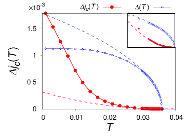
Figure 2: The temperature dependence of $\Delta j_{c}$ at $h=0.03$. The red closed circles indicate $\Delta j_{c}(T)$, while the open blue circles indicate $\Delta(T)$ (a.u.). The dashed lines show the fitting curve of $\Delta j_{c}(T)$ and $\Delta(T)$ near $T_{c}$ with $(T_{c}-T)^{2}$ and $\sqrt{T_{c}-T}$, respectively. The inset shows the enlarged figure near $T_{c}\simeq 0.036$.

Critical current under low fields. — Equipped with the insight of the GL theory, we discuss the temperature dependence of $\Delta j_{c}$ based on the model (1). The result is shown in Fig. 2 for $h=0.03$. As shown in the inset, the temperature scaling $\Delta j_{c}\propto(T_{c}-T)^{2}$ is confirmed near the transition temperature $T_{c}$. The scaling law becomes inaccurate as $T_{c}-T$ gets large, where $\Delta(T)$ also deviates from $\Delta(T)\propto\sqrt{T_{c}-T}$. Importantly, $\Delta j_{c}(T)$ is strongly enhanced at low temperatures.

To clarify the origin of the SDE, we show $j(q)$ by red lines in Figs. 3. In Fig. 3 (a) for $T=0.03\simeq T_{\rm c}$, $j(q)$ is a smooth curve and its tiny asymmetry gives rise to $\Delta j_{c}$, as is illustrated by the difference of the solid and dashed horizontal lines (indicating $j_{c+}$ and $-j_{c-}$). This is consistent with the GL picture where $\Delta j_{c}$ is caused by the asymmetry factors $\alpha_{3},\beta_{1}\neq 0$. Two curves, $j(q)$ and $-j(q)$, cross at $q_{0}<0$, indicating the helical superconductivity. In Fig. 3 (c), $\Delta(q)$ and the minimum excitation energy $\Delta E(q)$ are shown in addition to $j(q)$, by the blue and black lines, respectively. The superconducting state remains stable even after the spectrum becomes gapless, and reaches the maximum and minimum of $j(q)$ in the gapless region.

As shown in Fig. 3 (b), the dispersion of $j(q)$ at $T=0.001\ll T_{\rm c}$ is significantly different from that at $T=0.03$, and a large $\Delta j_{c}$ is realized. The maximum and minimum of $j(q)$ are achieved at the ends of the region where $j(q)$ is almost linear in $q$. These momenta approximately coincide with the Landau critical momenta, $q_{R}>0$ and $q_{L}<0$, i.e. the first $q$’s satisfying $\Delta E(q)=0$, as is clear from Fig. 3 (d). Actually, the depairing effect takes place after $q>q_{R}$ or $q<q_{L}$: The excited quasiparticles reduce $|j(q)|$ and $\Delta(q)$ and finally cause a first-order phase transition into the normal state. From these observations, we obtain the formula

$$\Delta j_{c}=n^{s}_{xx}(q_{R}+q_{L}-2q_{0})/2,$$ (5)

by using, e.g., $j_{c+}=n^{s}_{xx}(q_{R}-q_{0})/2$ with the superfluid weight $n_{xx}^{s}=2\partial_{q_{0}}j(q_{0})$. Thus, the nonreciprocal Landau critical momentum $q_{R}+q_{L}$ measured from $2q_{0}$ gives rise to the SDE at extremely low temperatures. As $T$ gets larger, the maximum and minimum of $j(q)$ deviate from $j(q_{R})$ and $j(q_{L})$, and Eq. (5) becomes no longer valid. The mechanism of the SDE at low temperatures is not captured by the GL theory.

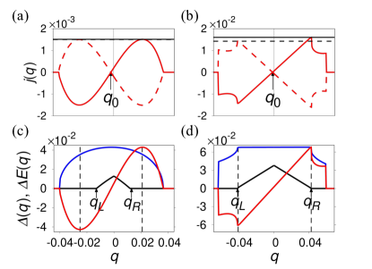
Figure 3: (a), (b): The $q$ dependence of the supercurrent at $h=0.03$ and (a) $T=0.03$ and (b) $T=0.001$. In addition to $j(q)$ (red lines), $-j(q)$ (dashed red lines) is shown. The black (dashed) horizontal lines indicate $j_{c+}$ ($-j_{c-}$). The position of $q_{0}$ is indicated by arrows. (c), (d): The order parameter $\Delta(q)$ (blue lines) and the excitation gap $\Delta E(q)$ (black lines) are shown together with $j(q)$ (a.u.). The parameters for the panels (c) and (d) are the same as the panel (a) and (b), respectively. The vertical dashed black lines indicate the momentum $q$ where $j(q)=j_{c\pm}$. Landau critical momentum $q_{R}$ and $q_{L}$ are indicated by arrows.

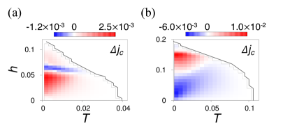
Figure 4: The magnetic-field and temperature dependence of the nonreciprocal component of the critical current $\Delta j_{c}(h,T)$ for (a) $t_{2}=0$ and (b) $t_{2}=0.2$. The red and blue colors indicate positive and negative values of $\Delta j_{c}$, respectively. The transition temperature $T_{c}(h)$ determined with the $T$ mesh (a) $0.045/21$ and (b) $0.12/21$ is shown with the black line for the guide of the eye.

Phase diagram. — In Figs. 4 (a) and (b), we show the temperature and magnetic-field dependence of the nonreciprocal component $\Delta j_{c}$ for $t_{2}=0$ and $t_{2}=0.2$. Let us focus on the low-field region, where positive and negative values of $\Delta j_{c}$ are widely obtained for Fig. 4 (a) and (b), respectively. The sign reversal of $\Delta j_{c}$ by $t_{2}$ can be understood based on Eq. (5). Indeed, we show in the Supplemental Material Sup that $q_{R}+q_{L}-2q_{0}$ causes a sign reversal as $t_{2}$ increases, leading to that of $\Delta j_{c}$ as well. It is also shown that for large values of $t_{2}$, $q_{R}+q_{L}-2q_{0}$ is dominated by the nonreciprocal Landau critical momentum $q_{R}+q_{L}$, while it is dominated by $-2q_{0}$ for small values of $t_{2}$. A relatively large SDE for $t_{2}\sim 0.2$ is explained by large values of $q_{R}+q_{L}-2q_{0}$ as a result of the anisotropy Sup . The pronounced aspect of Fig. 4 is the sign reversals prevailing under moderate and high magnetic fields. This point will be discussed in the following.

Critical current under high fields. —

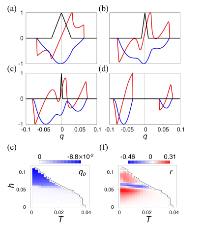
Figure 5: (a)-(d) $j(q)$ (red lines), $F(q)$ (blue lines), and $\Delta E(q)$ (black lines) normalized to $[-1,1]$ at $T=0.001$ for (a) $h=0.043$, (b) $h=0.058$, (c) $h=0.063$ and (d) $h=0.075$. (e),(f) $q_{0}$ and $r$ for various values of $h$ and $T$.

To see the origin of the high-field behavior, we show the condensation energy $F(q)$ at $T=0.001$ for various values of $h$ in Fig. 5. To be specific, the case of Fig. 4 (a) is considered. The condensation energy $F(q)$ shown by the blue line has a single-well structure under low magnetic fields [panel (a)]. The structure near $|q|\sim 0.05$ is developed under higher magnetic fields [panel (b)], to form two local minima [panel (c)], where the left one becomes most stable. These side wells are the precursor of the high-field helical superconducting states [panel (d)], where the central minimum finally disappears. Such a change is most evident in $q_{0}(T,h)$ shown in Fig. 5 (e). Under low fields, $q_{0}$ is determined by the balance of two Fermi surfaces shifted in the opposite directions, resulting in $|q_{0}|\lesssim 10^{-2}$; on the other hand, under high fields, $q_{0}\sim 10^{-1}$ almost coincides with $q_{\chi}$ of the Fermi surface with a larger density of states Dimitrova and Feigel’man (2003); Agterberg and Kaur (2007); Smidman et al. (2017); Yanase and Sigrist (2008). This determines the “crossover line” of helical superconductivity visible at $h\sim 0.06$ in Fig. 5 (e).

The evolution of $j(q)$ by $h$ follows that of $F(q)$. Overall, $j(q)$ consists of several almost-straight lines and their interpolation, since $F(q)$ is approximated by the square function of $q$ around each local minimum. Comparing Figs. 5 (a) and (b), the $q$ point achieving $j_{c-}$ is changed from $q_{L}$ to a critical momentum of the left well, which we name $q_{-,L}$. In the panel (c), $q_{-,L}$ remains to give $j_{c-}$, whose value is significantly enhanced owing to the development of the left minimum. This causes the sign reversal of $\Delta j_{c}$. In the panel (d), $\Delta j_{c}$ is determined by the tiny asymmetry of the left well. It should be noticed that the ratio $r=\Delta j_{c}/\bar{j}_{c}$ shown in Fig. 5 (f) is quite large around the crossover line, takes values up to $|r|\lesssim 0.4$, as is understood from Figs. 5 (a)-(c). Thus, the sign reversals and huge values of $r=\Delta j_{c}/\bar{j}_{c}$ under magnetic fields are caused by the change in the helical superconducting states. According to Figs. 5 (e) and (f), the sign reversal also occurs near $T_{c}(h)$ by the crossover.

Figure 4 (b) can be understood similarly. In this case, the crossover line is identified to be $h\sim 0.17$ Sup , where $\Delta j_{c}$ changes its sign. The high-field helical superconducting states span only a small fraction in the phase diagram. The difference from Fig. 4 (a) is another sign reversal at $h\sim 0.09$. In this region, $\Delta j_{c}$ is determined by the nonreciprocal Landau critical momentum, and $q_{R}+q_{L}-2q_{0}$ turns out to change its sign by increasing $h$. This is because $q_{R}+q_{L}(<0)$ shows nonmonotonic behavior, while $-2q_{0}(>0)$ grows linearly and finally becomes dominant Sup . The sign reversal survives at higher temperatures and reaches the transition temperature.

Discussion — We have revealed the sign reversals of the SDE, which is closely connected with the change in the helical superconducting states. Thus, the intrinsic SDE is a promising bulk probe directly unveiling the crossover line. This probe is complementary to the junction Kaur et al. (2005) and spectroscopy Smidman et al. (2017) experiments proposed to detect the helical superconductivity.

In the end, we briefly discuss the connection with the experimental results of SDE Ando et al. (2020). The sign reversals of $\Delta j_{c}$ by increasing the magnetic field at low temperatures have recently been observed Ono et al. , which might be explained by our results for the intrinsic SDE. An “inverse effect,” the nonreciprocity of the critical magnetic field under applied electric current, has also been reported Miyasaka et al. (2021), implying the nonreciprocity as a bulk property of the superconductor. Thus, the SDE with sign reversals implies the crossover in the superconducting state of the Nb/V/Ta superlattice. On the other hand, $\Delta j_{c}(h)$ near $T_{c}$ seems to be at variance with the intrinsic SDE Ando et al. (2020). This point might be overcome by considering the effect of vortices, which is left as an intriguing future issue.

I Formulation to evaluate the electric current

Here, we show the details of the formulation to calculate the current expectation values in the superconducting states. The free energy per unit volume in the superconducting state is given by

$$\Omega(\Delta,q) \equiv-\frac{T}{V}\ln\mathrm{Tr}\,e^{-\hat{H}_{\text{MF}}^{q}(\Delta)/T}$$

$$=\frac{1}{2V}\sum_{\bm{k}}\mathrm{tr}\,_{N}\left[\frac{\Delta^{2}}{U}+H_{N}(\bm{k})\right]$$

$$\qquad-\frac{T}{2V}\sum_{\bm{k}}\mathrm{tr}\,\left[\ln(1+e^{-H(\bm{k},q)/T})\right].$$ (6)

Here, $\mathrm{tr}\,_{N}$ represents the trace over the spin degrees of freedom, while $\mathrm{tr}\,$ represents that over both the spin and the Nambu degrees of freedom. $V=L_{x}L_{y}$ represents the system size with $L_{i}$ the diameter in the $i=x,y$ direction. We introduced the Bogoliubov-de Genens (BdG) Hamiltonian $H(\bm{k},q)$ by

$$\hat{H}_{\text{MF}}^{q}(\Delta)=\frac{1}{2}\sum_{\bm{k}}\Psi^{\dagger}(\bm{k},q)H(\bm{k},q)\Psi(\bm{k},q)+\text{const.},$$ (7)

$$H(\bm{k},q)=\begin{pmatrix}H_{N}(\bm{k}+\bm{q})&\Delta i\sigma_{y}\\ -\Delta i\sigma_{y}&-H_{N}^{T}(-\bm{k})\end{pmatrix},$$ (8)

with the momentum $\bm{q}=q\hat{x}$ and the Nambu spinor $\Psi(\bm{k},q)^{\dagger}=(c^{\dagger}_{\bm{k}+\bm{q}\uparrow},c^{\dagger}_{\bm{k}+\bm{q}\downarrow},c_{-\bm{k}\uparrow},c_{-\bm{k}\downarrow})$. Here, we choose $q$ to be compatible with the periodic boundary conditions, $q\in 2\pi\mathbb{Z}/L_{x}$. The constant term in Eq. (7) is equivalent to the first term of Eq. (6). The normal-state Bloch Hamiltonian is given by $H_{N}(\bm{k})=\xi(\bm{k})+(\bm{g}(\bm{k})-\bm{h})\cdot\bm{\sigma}$.

The electric current (the sheet current density) is defined by

$$j(\Delta,q)=\frac{\mathrm{tr}\,[\hat{j}_{x}e^{-\hat{H}^{q}_{\text{MF}}(\Delta)/T}]}{\mathrm{tr}\,[e^{-\hat{H}^{q}_{\text{MF}}(\Delta)/T}]}.$$ (9)

Here, the current operator is given by

$$\hat{j}_{x} =\frac{1}{V}\sum_{\bm{k}\sigma\sigma^{\prime}}\partial_{k_{x}}H_{N}(\bm{k})_{\sigma\sigma^{\prime}}c^{\dagger}_{\bm{k}\sigma}c_{\bm{k}\sigma^{\prime}}$$ (10)

$$=\frac{1}{V}\sum_{\bm{k}}\Psi^{\dagger}(\bm{k},q)\partial_{q}H(\bm{k},q)\Psi(\bm{k},q).$$ (11)

After some calculations, we obtain

$$j(\Delta,q) =\frac{1}{V}\sum_{\bm{k}}\mathrm{tr}\,[\partial_{q}H(\bm{k},q)f(H(\bm{k},q))]$$ (12)

$$=2\partial_{q}\Omega(\Delta,q),$$ (13)

with the Fermi distribution function $f(\epsilon)=(e^{\epsilon/T}+1)^{-1}$.

The gap equation is given by

$$\partial_{\Delta}\Omega(\Delta,q)=0,$$ (14)

which determines the pair potential $\Delta$ self-consistently. The solution is written as $\Delta(q)$, and satisfies Eq. (14), or equivalently,

$$\Delta(q)=-\frac{U}{V}\sum_{k}\braket{c_{-k\downarrow}c_{k+q\uparrow}}|_{\Delta=\Delta(q)}.$$ (15)

By using $\Delta(q)$, the condensation energy defined in the main text is written as

$$F(q)=\Omega(\Delta(q),q)-\Omega(0,q),$$ (16)

where $\Omega(0,q)=\Omega(0,0)$ holds as is easily confirmed with Eqs. (6) and (8). By using Eqs. (13) and (14), we obtain

$$2\partial_{q}F(q) =\lim_{\Delta\to\Delta(q)}\bigl{[}2\partial_{q}\Omega(\Delta,q)+2\partial_{q}\Delta(q)\,\partial_{\Delta}\Omega(\Delta,q)\bigr{]}$$

$$=j(\Delta(q),q)$$

$$\equiv j(q).$$ (17)

The obtained equality goes along with the standard expression $j=-\partial_{A}\Omega$ with $A$ the uniform vector potential since $q$ changes by $-2\delta A$ when $A$ changes by $\delta A$.

II GL analysis

Here we show the details of the GL analysis of the superconducting diode effect. Let us start from the expression

$$f(\Delta,q)=\alpha(q)\Delta^{2}+\frac{\beta(q)}{2}\Delta^{4},$$ (18)

keeping the order parameter of the form $\Delta(x)\propto e^{iqx}$ in mind. The coefficients are given by

$$\alpha(q)=-{\tilde{\alpha}}_{0}+\frac{{\tilde{\alpha}}_{2}}{2}(q-q_{0})^{2}+\frac{\alpha_{3}}{6}(q-q_{0})^{3},$$

$$\beta(q)={\tilde{\beta}}_{0}+\beta_{1}(q-q_{0}).$$ (19)

Here we omit the tilde of $\tilde{q}_{0}$ in the main text for simplicity, and redefine ${\tilde{\alpha}}_{0}\to-{\tilde{\alpha}}_{0}$. The order parameter is optimized by

$$\partial f/\partial{\Delta^{2}}=\alpha(q)+\beta(q)\Delta^{2}=0.$$ (20)

Assuming $\beta(q)>0$ for the range of $q$ we are interested in, $\Delta$ has a nontrivial real solution only when $\alpha(q)<0$. Thus, the GL free energy is given by

$$f(q)=f(\Delta(q),q)=-\frac{\alpha(q)^{2}}{2\beta(q)}\theta(-\alpha(q)),$$ (21)

with $\theta(x)$ the Heaviside step function. Since the minimum of $\alpha(q)$ is $-{\tilde{\alpha}}_{0}$, the transition from the normal to helical superconducting state occurs when the sign of ${\tilde{\alpha}}_{0}$ changes from negative to positive as lowering the temperature. Thus, we conclude ${\tilde{\alpha}}_{0}\propto T_{c}-T$.

We first consider the case $\alpha_{3}=\beta_{1}=0$. The supercurrent is given by $j(q)=2\partial_{q}f(q)$,

$${\tilde{\beta}}_{0}j(q)/2=-\partial_{q}\alpha(q)^{2}/2=-\alpha(q)\partial_{q}\alpha(q).$$ (22)

This is an odd function of $q-q_{0}$, and thus the critical current is reciprocal. Actually, The maximum and minimum of $j(q)$ are achieved at $q=q_{c}$ satisfying

$$0 =[\partial_{q_{c}}{\tilde{\beta}}_{0}j(q_{c})/2]_{\alpha_{3}=\beta_{1}=0}$$

$$=\frac{3{\tilde{\alpha}}_{2}^{2}}{2}\left(\frac{2{\tilde{\alpha}}_{0}}{3{\tilde{\alpha}}_{2}}-(q_{c}-q_{0})^{2}\right).$$ (23)

Accordingly, $|q_{c}-q_{0}|$ scales as $\sqrt{T_{c}-T}$, as is the inverse of the coherence length. Thus, the reciprocal critical current is given by

$$[j_{c+}]_{\alpha_{3}=\beta_{1}=0} =[-j_{c-}]_{\alpha_{3}=\beta_{1}=0}$$

$$=\frac{4\sqrt{6{\tilde{\alpha}}_{2}}}{9{\tilde{\beta}}_{0}}{\tilde{\alpha}}_{0}^{3/2}.$$ (24)

Note that this coincides with $\bar{j}_{c}$ up to first order in $\alpha_{3}$ and $\beta_{1}$. Thus, the well-known scaling law $j_{c}\sim(T_{c}-T)^{3/2}$ is reproduced for $\bar{j}_{c}$.

Let us consider the first-order change caused by $\alpha_{3}$ and $\beta_{1}$. We obtain

$$\partial_{\alpha_{3}}[{\tilde{\beta}}_{0}j(q)/2]\Bigr{|}_{\alpha_{3}=\beta_{1}=0}$$

$$=\frac{5{\tilde{\alpha}}_{2}(q-q_{0})^{2}}{12}\left(\frac{6{\tilde{\alpha}}_{0}}{5{\tilde{\alpha}}_{2}}-(q-q_{0})^{2}\right),$$ (25)

and

$$\partial_{\beta_{1}}[{\tilde{\beta}}_{0}j(q)/2]\Bigr{|}_{\alpha_{3}=\beta_{1}=0}$$

$$=\frac{5{\tilde{\alpha}}_{2}^{2}}{8{\tilde{\beta}}_{0}}\left((q-q_{0})^{2}-\frac{2{\tilde{\alpha}}_{0}}{{\tilde{\alpha}}_{2}}\right)\left((q-q_{0})^{2}-\frac{2{\tilde{\alpha}}_{0}}{5{\tilde{\alpha}}_{2}}\right).$$ (26)

When the critical current $j_{c+}$ is realized at $q_{c+}=q_{c}+\delta q_{c}$, we obtain up to first order in $\alpha_{3}$ and $\beta_{1}$,

$$j(q_{c+}) =[j+\delta j](q_{c}+\delta q_{c})$$

$$=j_{c0}+\alpha_{3}[\partial_{\alpha_{3}}j(q_{c})]_{\alpha_{3}=\beta_{1}=0}$$

$$\quad+\beta_{1}[\partial_{\beta_{1}}j(q_{c})]_{\alpha_{3}=\beta_{1}=0}$$

$$\quad+[\partial_{q_{c}}j(q_{c})]_{\alpha_{3}=\beta_{1}=0}\delta q_{c}$$

$$=j_{c0}+\alpha_{3}[\partial_{\alpha_{3}}j(q_{c})]_{\alpha_{3}=\beta_{1}=0}$$

$$\quad+\beta_{1}[\partial_{\beta_{1}}j(q_{c})]_{\alpha_{3}=\beta_{1}=0}.$$ (27)

Here, $j_{c0}$ represents $[j(q_{c})]_{\alpha_{3}=\beta_{1}=0}$. Thus, we obtain the nonreciprocal component of the critical current,

$$\Delta j_{c} =2\alpha_{3}[\partial_{\alpha_{3}}j(q_{c})]_{\alpha_{3}=\beta_{1}=0}+2\beta_{1}[\partial_{\beta_{1}}j(q_{c})]_{\alpha_{3}=\beta_{1}=0}$$

$$=\frac{16{\tilde{\alpha}}_{0}^{2}}{27{\tilde{\beta}}_{0}{\tilde{\alpha}}_{2}}\alpha_{3}-\frac{8{\tilde{\alpha}}_{0}^{2}}{9{\tilde{\beta}}_{0}^{2}}\beta_{1}.$$ (28)

This scales as $\Delta j_{c}\sim(T_{c}-T)^{2}$.

(a)	(b)	(c)	(d)

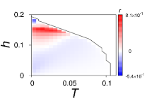
Figure 6: Temperature and magnetic-field dependence of (a),(b) $\Delta E$, (c) $q_{0}$, and (d) $r$. $t_{2}=0$ for the panel (a), while $t_{2}=0.2$ for the panels (b)-(d).

III Calculation details and Phase diagrams

Here we explain the details of the numerical calculations and show some additional figures related to the phase diagrams. All the calculations for the figures in the main text and those presented here are done with $L_{x}=6000$ and $L_{y}=200$. Exceptionally, we adopt $L_{x}=12000$ for Fig. 5 and $T>0.03$ in Fig. 2 to reduce the finite-size effect. To obtain $j_{c\pm}$, $j(q)$ is maximized/minimized among $q\in 2\pi\mathbb{Z}/L_{x}$. The normalization of Figs. 5 (a)-(d) is done with $\max[j_{c+},|j_{c-}|]$, $|\min_{q}F(q)|$, and $\max[0.003,\max_{q}\Delta E(q)]$ for $j(q)$, $F(q)$, and $\Delta E(q)$, respectively. Note that we show in Figs. 5 (a)-(d) only the most stable state that minimizes $F(q)$ for each $q$. In particular, there is a metastable superconducting state for smaller (larger) $q$’s of the left (right) peaks in Fig. 5 (d). The supercurrent sustained by these states might be observed when the experimental time scale is small. For Figs. 5 (a)-(d), it is confirmed that the superconducting solution is (if any) unique for each $q$.

In Figs. 6 (a) and (b), we show the temperature and magnetic-filed dependence of the minimum excitation energy $\Delta E(q_{0})$ for $t_{2}=0$ and $0.2$, respectively. The spectrum becomes gapless in the high-field helical superconducting states, which can be detected by scanning tunneling microscopy. Figures 6 (c) and (d) show $q_{0}$ and $r$ for $t_{2}=0.2$. In Figs. 6 (c) and (d), the crossover line is seen to be $h\sim 0.17$, and a huge nonreciprocal nature $r\sim 0.8$ is observed. To be precise, $\Delta j_{c}$ becomes positive in a tiny region near $h\sim 0.19$ and $T\sim 0$ for $t_{2}=0.2$. However, this is probably due to the peculiarity of the model, where the Lifshitz transition of the outer Fermi surface occurs around $h\sim 0.185$.

IV Evolution of Landau critical momenta

As discussed in the main text, the sign reversal of $\Delta j_{c}$ by $t_{2}$ can be understood based on the nonreciprocity of the Landau critical momenta. In Fig. 7, we show $q_{R}+q_{L}$ and $q_{0}$ obtained from $j(q)$ at $h=0.03$ and $T=0.001$, with varying $t_{2}$ from $0$ to $0.2$. The sign reversal of $q_{R}+q_{L}-2q_{0}$ (red closed circles) naturally explains that of $\Delta j_{c}$. For large values of $t_{2}$, $q_{R}+q_{L}-2q_{0}$ is dominated by the nonreciprocal Landau critical momentum $q_{R}+q_{L}$ (blue closed triangles), while it is dominated by $q_{0}$ (black closed squares) for small values of $t_{2}$. It should be noted that a large SDE is obtained for $t_{2}\sim 0.2$, although $q_{R}+q_{L}$ and $-2q_{0}$ contribute destructively.

To understand the behavior of $q_{R}+q_{L}$, we discuss the Landau critical momenta with the help of the single-band formula $|\bm{q}\cdot\bm{v}/2|=\Delta$. In our case, $\bm{q}$ should be replaced with $\bm{q}-\bm{q}_{\chi}(\bm{k})$ for each band, and we obtain,

$$\Delta =\max_{\chi=\pm,\ \bm{k}=\bm{k}_{F}^{\chi}}\left|\frac{q\,\hat{x}-\bm{q}_{\chi}(\bm{k})}{2}\cdot\bm{v}_{\chi}(\bm{k})\right|$$

$$=\max_{\chi=\pm,\ \bm{k}=\bm{k}_{F}^{\chi}}\left|qv_{\chi,x}(\bm{k})/2-\chi h\hat{g}_{y}(\bm{k})\right|,$$ (29)

whose positive and negative solutions for $q$ correspond to $q_{R}$ and $q_{L}$, respectively. Here, $\bm{k}_{F}^{\chi}$ specifies the $\bm{k}$ points on the Fermi surface with the helicity $\chi$, while $\hat{g}(\bm{k})$ is the unit vector parallel to $\bm{g}(\bm{k})$. Equation (29) well reproduces the result for $q_{R}+q_{L}$, as shown by skyblue open triangles in Fig. 7. To go further, let us simplify the expression by replacing $\bm{q}_{\chi}(\bm{k})$ in the first line of Eq. (29) with its average on the Fermi surface: $q_{\chi}\hat{x}\equiv\braket{\bm{q}_{\chi}(\bm{k}_{F,\chi})}$. We obtain for $h>0$ [see the next section for the derivation],

$$q_{R}+q_{L} =\begin{cases}\begin{array}[]{l}q_{+}+q_{-}\\ \ +2\left(\frac{\Delta}{v_{-}}-\frac{\Delta}{v_{+}}\right),\end{array}&(|\delta v|/\bar{v}\lesssim h/\Delta)\\ 2q_{+},&(\delta v/\bar{v}\gtrsim h/\Delta)\\ 2q_{-},&(\delta v/\bar{v}\lesssim-h/\Delta)\end{cases}$$ (30)

whose helicities are interchanged for $h<0$. Here, we defined $v_{\chi}\equiv\max_{\bm{k}_{F}^{\chi}}v_{\chi,x}(\bm{k}_{F}^{\chi})$, $\delta v=v_{+}-v_{-}$ and $\bar{v}\sim(v_{+}+v_{-})/2$. Equation (30) qualitatively agrees with $q_{R}+q_{L}$ for $t_{2}\lesssim 0.15$, as shown by the open purple inverted triangles in Fig. 7. In this regime, we have small $\delta v$ and the first line of Eq. (30) is applied. Since $q_{\pm}\sim\pm 2h/v_{\pm}$, the difference of the Fermi velocities $\delta v$ plays a key role to obtain a large $q_{R}+q_{L}$. It is expected that the anisotropy of the system is advantageous to obtain a large value of $\delta v$. On the other hand, Eq. (30) underestimates $q_{R}+q_{L}$ around $t_{2}=0.2$, where the third line of Eq. (30) is applied. This indicates that the isotropic simplification $\bm{q}_{\chi}(\bm{k})\to q_{\chi}$ is not valid for strongly anisotropic systems with large $t_{2}$. Thus, overall, large anisotropy of the system is expected to be the key to obtain a large SDE.

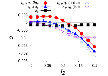
Figure 7: $t_{2}$ dependence of $q_{R}+q_{L}$, $q_{0}$, and their combinations. The red closed circles, blue closed triangles, black closed squares indicate $q_{R}+q_{L}-2q_{0}$, $q_{R}+q_{L}$, $q_{0}$ evaluated from $j(q)$, respectively. The open sky-blue triangles and open purple inverted triangles indicate $q_{R}+q_{L}$ calculated from Eq. (29) and that with the isotropic simplification $\bm{q}_{\chi}(\bm{k})\to q_{\chi}\hat{x}$, respectively.

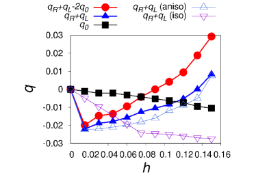
Figure 8: Magnetic field dependence of $q_{R}+q_{L}$, $q_{0}$ and their combinations for $t_{2}=0.2$ and $T=0.001$. The notations are the same as Fig. 7.

In Fig. 8, we show the magnetic-field dependence of $q_{R}+q_{L}$, $q_{0}$ and their combinations for $t_{2}=0.2$. The notations are the same as those of Fig. 7. While $q_{R}+q_{L}$ is nonmonotonic, $-2q_{0}$ grows linearly and finally the sign reversal of $q_{R}+q_{L}-2q_{0}$ occurs. “$q_{R}+q_{L}$ (aniso)”, i.e. Eq. (29), qualitatively captures the behavior of $q_{R}+q_{L}$, whose slight deviation is probably due to the higher-order corrections of $h$. The isotropic simplification does not work for $t_{2}=0.2$ as is clear in Fig. 8. The sign reversal of $q_{R}+q_{L}-2q_{0}$ is the origin of that of $\Delta j_{c}$ in the phase diagram for $t_{2}=0.2$ under moderate magnetic fields.

IV.1 Derivation of Eq. (30)

Here, we derive Eq. (30). By using $\bm{q}_{\chi}(\bm{k})\to q_{\chi}\hat{x}$, we obtain

$$2\Delta =\max_{\chi=\pm}\Bigl{[}|q-q_{\chi}|\max_{\bm{k}_{F}^{\chi}}|v_{\chi,x}(\bm{k})|\Bigr{]}$$ (31)

$$=\max_{\chi=\pm}\Bigl{[}|q-q_{\chi}|v_{\chi}\Bigr{]}.$$ (32)

Let us first consider the positive solution $q=q_{R}>0$. We also fix $h>0$. Then, we obtain

$$2\Delta =\max\Bigl{[}(q_{R}+|q_{-}|)v_{-},\,(q_{R}-|q_{+}|)v_{+}\Bigr{]}.$$ (33)

When $(q_{R}+|q_{-}|)v_{-}>(q_{R}-|q_{+}|)v_{+}$, we obtain

$$q_{R}=q_{-}+\frac{2\Delta}{v_{-}}.$$ (34)

The consistency can be checked as follows. The above inequality reads

$$\delta vq_{R}<|q_{-}|v_{-}+|q_{+}|v_{+}\sim 2h.$$ (35)

Thus, this solution is valid for

$$2h\gtrsim\delta v\frac{2(\Delta-h)}{v_{-}}\sim\frac{2\delta v(\Delta-h)}{\bar{v}}.$$ (36)

Considering only the linear dependence in $h$, we obtain

$$q_{R}=q_{-}+\frac{2\Delta}{v_{-}},\quad\frac{\delta v}{\bar{v}}\lesssim\frac{h}{\Delta}.$$ (37)

In the same way, we obtain

$$q_{R}=q_{+}+\frac{2\Delta}{v_{+}},$$ (38)

for $\delta vq_{R}\gtrsim 2h$, i.e. $\delta v/\bar{v}\gtrsim h/\Delta$. The negative solutions $q=q_{L}<0$ are obtained as follows:

$$q_{L}=\begin{cases}q_{+}-\frac{2\Delta}{v_{+}},&\frac{\delta v}{\bar{v}}\gtrsim\frac{-h}{\Delta}\\ q_{-}-\frac{2\Delta}{v_{-}}.&\frac{\delta v}{\bar{v}}\lesssim\frac{-h}{\Delta}\end{cases}$$ (39)

Summing up $q_{R}$ and $q_{L}$, we obtain Eq. (30).