Control-Oriented Model-Based Reinforcement Learning with Implicit Differentiation
Abstract
The shortcomings of maximum likelihood estimation in the context of model-based reinforcement learning have been highlighted by an increasing number of papers. When the model class is misspecified or has a limited representational capacity, model parameters with high likelihood might not necessarily result in high performance of the agent on a downstream control task. To alleviate this problem, we propose an end-to-end approach for model learning which directly optimizes the expected returns using implicit differentiation. We treat a value function that satisfies the Bellman optimality operator induced by the model as an implicit function of model parameters and show how to differentiate the function. We provide theoretical and empirical evidence highlighting the benefits of our approach in the model misspecification regime compared to likelihood-based methods.
1 Introduction
The conceptual separation between model learning and policy optimization is the basis for much of the work on model-based reinforcement learning (MBRL) [28, 73, 53, 12, 17, 33, 40, 44]. A standard MBRL agent first estimates the transition parameters and the reward function of a Markov Decision Process and then uses the approximate model for planning [77, 49, 56, 27, 13, 37, 57, 69]. If the estimated model perfectly captures the actual system, the resulting policies are not affected by the model approximation error. However, if the model is imperfect, the inaccuracies can lead to nuanced effects on the policy performance [2, 57]. Several works [71, 43, 50] have pointed out on the objective mismatch in MBRL and demonstrated that optimization of model likelihood might be unrelated to optimization of the returns achieved by the agent that uses the model. For example, accurately predicting individual pixels of the next state [44] might be neither easy nor necessary for decision making. Motivated by these observations, our paper studies control-oriented model learning that takes into account how the model is used by the agent.
While much of the work in control-oriented model learning has focused on robust or uncertainty-based methods [55, 61, 39, 82, 83], we propose an algorithm for learning a model that directly optimizes the expected return using implicit differentiation [16, 29]. Specifically, we assume that there exists an implicit function that takes the model as input and outputs a value function that is a fixed point of the Bellman optimality operator [20] induced by the model. We then calculate the derivatives of the optimal value function with respect to the model parameters using the implicit function theorem (IFT), allowing us to form a differentiable computational graph from model parameters to the sum of rewards. In reference to [67, 72, 7], we call our control-oriented method optimal model design (OMD).
Our contributions can be summarized as follows:
-
•
We propose OMD, an end-to-end MBRL method that optimizes expected returns directly.
-
•
We characterize the set of OMD models in the tabular case and derive an approximation bound on the optimal value function that is tighter than the likelihood-based bound.
-
•
We propose a series of approximations to scale our approach to non-tabular environments.
-
•
We demonstrate that OMD outperforms likelihood-based MBRL agents under the model misspecification in both tabular and non-tabular settings. This finding suggests that our method should be preferred when we cannot approximate the true model accurately.
-
•
We empirically demonstrate that models obtained by OMD can have lower likelihood than a random model yet generate useful targets for updating the value function. This finding suggests that likelihood optimization might be an unnecessary step for MBRL.

2 Related work
Learning control-oriented models.
Earlier work in optimal control and econometrics [71, 67] studied the relation between the model approximation error and the control performance and noted that true parameter identification could be suboptimal when the model class is limited. Joseph et al. [43] were one of the first to address the objective mismatch [50] and proposed an algorithm for training models that maximize the expected returns using zero-order optimization.
Several papers have proposed model learning approaches that optimize other return-aware objectives. Farahmand et al. [23] train a model to minimize the difference between values of the real next states and the next states predicted by the dynamics. Abachi et al. [1] use the norm of the difference between policy gradients as the model objective. D’Oro et al. [22] use a weighted maximum likelihood objective where the weights are chosen to minimize the difference between the true policy gradient and the policy gradient in the MDP induced by the model. Schrittwieser et al. [70] use tree search and train a model for image-based states by encoding them into a latent space and predicting a reward, a policy, and values without reconstructing the images.
The idea of differentiable planning has also been investigated. Amos et al. [4] learn a model via differentiating the Karush–Kuhn–Tucker conditions in the LQR setting [21]. Tamar et al. [76] uses a differentiable approximation of the value iteration algorithm to learn a planner. Amos and Yarats [3] optimize the parameters of a sampling distribution in Cross-Entropy Method [66] using a differentiable approximation of Top-K operation.
Several works have theoretically studied the control-oriented model learning. Ayoub et al. [5] derive regret bounds for models used to predict values. Grimm et al. [30] introduce the principle of value equivalence for MBRL defining two models to be equivalent if they induce the same Bellman operator.
Our work is closely related to the above papers but proposes to learn models by directly optimizing the sum of rewards in an end-to-end manner via gradient-based methods.
Implicit function theorem.
Implicit differentiation has been applied for a variety of bi-level optimization problems. Lorraine et al. [54] treat weights of a neural network as an implicit function of hyperparameters and use IFT to optimize the hyperparameters. Rajeswaran et al. [64] study meta-learning and apply IFT to compute the outer loop gradient without the need to differentiate through the inner loop iterations. Instead of treating a neural network as a sequence of layers that transform an input, Bai et al. [8] propose an implicit layer that corresponds to an infinite depth neural network and find a fixed point of the layer via IFT. Our method also solves a bi-level problem: in the inner loop, we train an action-value function compatible with the model, while in the outer loop we update the model parameters towards maximizing the expected returns.
3 Preliminaries
Reinforcement Learning (RL) [74] methods follow the Markov Decision Process (MDP) formalism. An MDP is defined as , where is a state space, is an action space, is a transition probability distribution (often called dynamics), is a reward function, is a discount factor, and is an initial state distribution. The pair (, ) is jointly called the true model. The goal of an agent is to learn a policy that maximizes the expected discounted sum of rewards . The performance of the agent following the policy can also be quantified using the action value function .
Model-based RL algorithms typically train a model (, ) and use it for policy or value learning. Traditional methods based on Dyna [73] rely on maximum likelihood estimation (MLE) of model parameters . For example, if the true model is assumed to be Gaussian with a parameterized mean and a fixed variance, maximizing the likelihood is equivalent to minimizing the mean squared error of the prediction, namely, to solving
| (1) |
4 Optimal Model Design for Tabular MDPs
Consider a modification of the original RL problem statement, which was first proposed by Rust [67] and revisited by Bacon et al. [7]. In addition to maximizing the expected returns , we introduce a constraint forcing the action value function to satisfy the Bellman equation induced by the model. The optimization problem becomes
| (2) |
is the soft Bellman optimality operator with respect to the model and is the softmax policy:
| (3) |
We choose the soft Bellman operator with over the “hard” version with because of the differentiability of log-sum-exp. We also use a temperature in softmax and log-sum-exp but omit it from the expressions for simplicity. Note that finding a fixed point of the soft Bellman optimality operator corresponds to solving the MaxEnt RL formulation [84], but for a sufficiently small value of , the difference is negligible.111More details about the soft Bellman operator and MaxEnt RL could be found in [51].
Suppose there exists an implicit function that takes as input a model and outputs a Q-function that satisfies the constraint in (2). The sequence of transformations from the model parameters to the agent’s performance can be described then using the following graph:
| (4) |
In Section 4.1, we show how can be calculated using the implicit function theorem (IFT). Since can be calculated using the policy gradient theorem [75], we can apply automatic differentiation to calculate the gradient with respect to :
| (5) |
Given the expression for the gradient of with respect to , we use an appropriate optimization method to train the model. We call the approach optimal model design (OMD). Note that Dyna-based methods also train the Q-function to satisfy the constraint in (2) while using the likelihood as the objective for model parameters [65]. In contrast, we train to directly optimize the expected returns.
The optimization problem (2) suggests that OMD is a policy-based method [75]. However, we can turn it into a value-based approach [81] by replacing the objective with the Bellman error:
| (6) |
where , similarly to , is the soft Bellman operator but induced by the true reward and dynamics . We discuss the relation between the models obtained by solving problems (2) and (6) in Section 5.1.
While the constraint has to be satisfied for all state-action pairs limiting the approach to tabular MDPs, we show an extention to the function approximation case in Section 6.
4.1 Implicit Differentiation
In this subsection, we state the implicit function theorem used to calculate .
Theorem 1.
(Cauchy, Implicit Function)
Let be a continuously differentiable function and be a point satisfying . If the Jacobian is invertible, then there exists an open set containing and a unique continuously differentiable function such that and for all . Moreover,
| (7) |
We provide a proof in Appendix B. Note that (7) requires only a final point satisfying the constraint and does not require knowledge about itself. Hence, can be any black-box function outputting . The gradient of the scalar objective or is calculated using (7). To use backpropagation, we only need to define the product of a vector and . We provide an implementation of a custom vector-Jacobian product for the implicit function in Appendix A allowing to use as a block in a differentiable computational graph.
4.2 Benefits under Model Misspecification
In the previous subsection, we showed how to use implicit differentiation for training a model that aims to maximize the expected returns. In this subsection, we demonstrate that such a control-oriented model is preferable over a likelihood-based in the setting where the true model is not representable by a chosen parametric class.
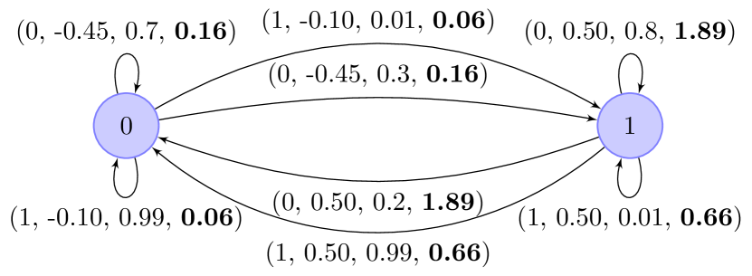
Let and be a parametric model, where parameters in denote the corresponding logits and each parameter in is a reward for a state-action pair. We consider a set of parameters with the bounded norm and use as a measure of the model misspecification. By decreasing the bound of the norm of , we get a more misspecified model class. To isolate the model learning aspect, we consider the exact RL setting without sampling. We take a 2 state, 2 action MDP shown in Figure 3 with a discount factor and a uniform initial distribution . For every , a function outputs the corresponding via performing the fixed point iteration until convergence. is transformed into the policy via softmax with the temperature . Given the policy , we calculate in a closed form [74].
For OMD, we obtain the gradient of with respect to using the expression (5). We then apply the projected gradient ascent where after each step we make a projection on a space of bounded parameters via clipping to if . Finding an MLE solution corresponds to minimizing the average KL divergence
for optimizing and minimizing the squared error for . We similarly perform the projected gradient descent and call the agent MLE (despite having the exact setting without estimation).
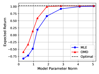
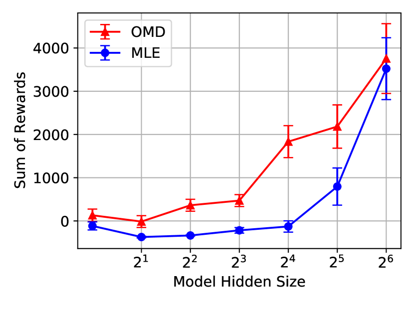
The resulting as a function of the norm bound is shown in Figure 2. When the true model is not representable by a chosen class, OMD learns a model that uses its representational capacity for helping the agent to maximize the expected returns, while the MLE agent tries to predict the next states and rewards accurately while discarding the true objective function the agent seeks to optimize.
In MDPs with high-dimensional state spaces [11, 10] where the underlying dynamics are complex, having a model that will accurately predict the next observation might be expensive and unnecessary for decision making. Figure 2 reflects the problems an MLE-based model will face for such environments and provides evidence for using control-oriented models that leverage the available capacity of the model more effectively.
5 Theoretical Analysis
In the previous section, we have empirically demonstrated that OMD outperforms Dyna-style [73] MBRL agents when the model capacity is limited. This section characterizes the set of optimal solutions of OMD and compares the approximation bounds for OMD and MLE agents.
5.1 Optimal Solutions for OMD
We use the principle of value equivalence for MBRL [30] and argue that value equivalent models are optimal solutions to (2) and (6).
Definition 1 (Optimal value equivalence).
Let be an optimal action-value function for the unconstrained RL problem. The models with parameters and are -equivalent if
| (8) |
The definition is a slight modification of the value equivalence used in [30]: instead of requiring the Bellman operators to be equal for a set of value functions and policies, we require the equality for a chosen only. The subset of models that are -equivalent forms an equivalence class .
Proposition 1.
This property holds by construction. The optimal Q-function maximizes the objective in the true MDP. As the log-sum-exp temperature in (3) approaches 0, we recover the “hard” target in the Bellman optimality operator:
| (9) |
Thus, if we set to the true model, will satisfy the Bellman equation . But even though the true model belongs to the equivalence class , it is not identifiable: all models from are going to be indistinguishable for OMD. Seemingly undesirable at first glance, it allows OMD choosing any model that induces the same Bellman operator, which is beneficial under the model misspecification as shown in Section 4.2.
We provide an example of a model that is -equivalent with the true model in Figure 3. The model differs significantly, demonstrating that the equivalence class consists of multiple elements. Moreover, the dynamics learned by OMD are deterministic, suggesting that OMD can choose a simpler model that will have the same as the true model. Drawing the connection to the prior work on state abstractions [52], the fact that MDPs have the same optimal action values indicates that the learned models can be seen as -irrelevant with respect to a state abstraction over .

5.2 Approximation Bound
Our next result relates approximation errors for the optimal Q-functions under the OMD and MLE models. For simplicity, we analyze the setting with and the Bellman error (6) as the objective.
Theorem 2.
( approximation error) Let be the optimal action-value function for the true MDP. Let and be the fixed points of the Bellman optimality operators for approximate OMD and MLE models respectively. Then,
-
•
If the MLE dynamics and reward have the bounded errors and , and the reward function is bounded , we have
-
•
If the Bellman optimality operator induced by the OMD model has the bounded error , we have
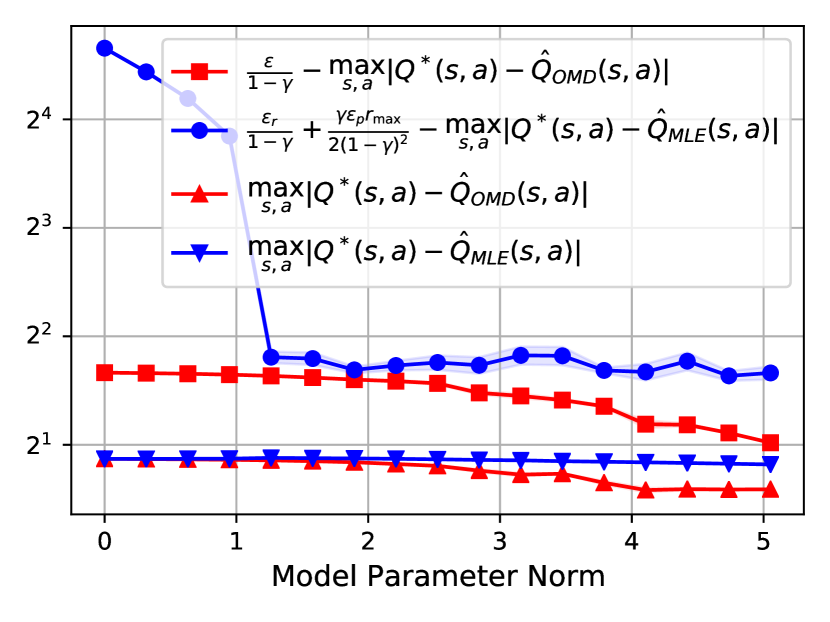
We prove the bounds in Appendix G using similar arguments as the proof of the simulation lemma [46]. The MLE bound has a term making the bound loose compared to the OMD bound with only the term. The bound suggests that OMD approximation error translates into a lower approximation error than for the MLE model. Figure 3 compares empirically the errors and the tightness of the bounds for a tabular MDP where can be computed exactly. The result provides evidence that OMD indeed achieves a lower approximation error compared to an agent that seeks to estimate and accurately. Motivated by the theoretical findings, the next section discusses a practical version of OMD.
6 OMD with Function Approximation
Section 4 describes optimal model design, a non-likelihood-based method for learning models in tabular MDPs. In this section, we propose several approximations to make OMD practically applicable. We analyze the effect of the approximations and perform an ablation study in Appendix E.
Q-network. We use a neural network with parameters to approximate the Q-values. The network is trained to minimize the Bellman error induced by the model :
| (10) |
where is a target copy of parameters updated using exponential moving average, a standard practice to increase the stability of deep Q-learning [59]. We also use double Q-learning [35, 25] but omit it from the equations for simplicity. To estimate the expectation, we use a replay buffer [59].
Constraint. The constraint in (2) and (6) should be satisfied for all state-action pairs making it impractical for non-tabular MDPs. We introduce an alternative but similar constraint, the first-order optimality condition for minimizing the Bellman error (10):
Implicit differentiation. The process of training is bi-level: in the inner loop, we optimize the Q-function parameters to get optimal corresponding to a fixed model ; in the outer loop, we make a gradient update of . We make steps of an optimization method to approximate where is a hyperparameter and reuse the weights from the previous outer loop iterations. We follow Rajeswaran et al. [65] and approximate the inverse Jacobian term in with the identity matrix. Surprisingly, we did not observe benefits when using the inverse Jacobian term. We investigate the phenomenon deeper and discuss possible explanations in Appendix C.
Objective. We consider the problem (6) and use the Bellman error as the outer loop objective:
| (11) |
where , again, is the soft Bellman optimality operator induced by the true reward and dynamics .
Note that the objective (11) is used for estimating the gradient with respect to only and is trained to optimize . While both and objectives could be used for training , we found that the latter requires more samples to converge. Note that optimizing the still corresponds to maximizing the (entropy-regularized) expected returns.
Resulting gradient. The changes above in the objective function and the constraint yield the following optimization problem:
| (12) |
The Q-function and IFT approximations and result in the following gradient with respect to the model parameters:
| (13) |
The OMD algorithm is summarised in Algorithm 1. The only difference between Dyna-based approaches and OMD (highlighted in blue) is given by the gradient used to train model parameters .
7 Experiments with Function Approximation
This section aims to test the following hypotheses:
-
•
The OMD agent with approximations from Section 6 achieves near-optimal returns.
-
•
The performance of OMD is better compared to MLE under the model misspecification.
-
•
The parameters of the OMD model have low likelihood, yet the agent that acts using the Q-function trained with the model achieves near-optimal returns in the true MDP.
Setup. We provide full details about the experimental setup and hyperparameters in Appendix D. We choose CartPole [9] to have controllable experiments but also include results on MuJoCo HalfCheetah [78] with similar findings in Appendix F further supporting our conclusions. Since OMD learns one of the -equivalent models as shown in Section 5.1, a close non-MLE baseline would be the algorithm used in the value equivalence principle (VEP) paper [30]. The VEP model minimizes the difference between the Bellman operators:
| (14) |
where , is the real model counterpart estimated from samples, and and are predefined sets of policies and value functions.
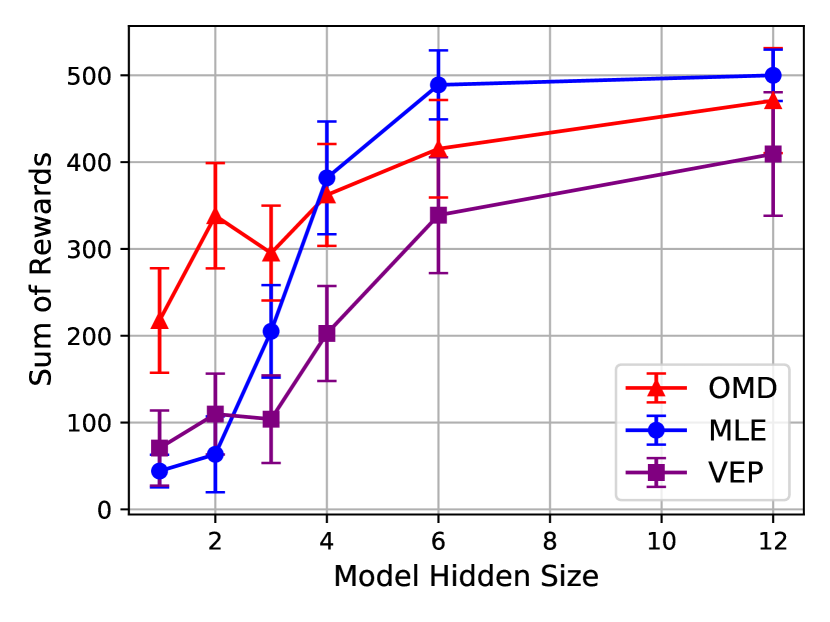
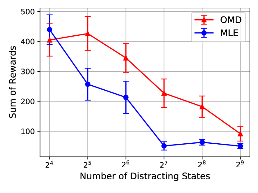
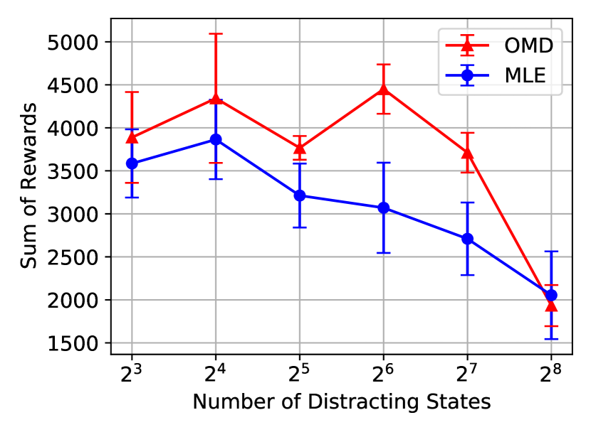
Performance under model misspecification. We design two experiments that allow measuring the misspecification in isolation. First, we limit the model class representational capacity by controlling the number of units in hidden layers of the model. Next, we add distracting states by sampling noise from a standard gaussian and vary the number of distractors. Figure 4 shows the returns achieved by the agents after training in the two regimes. Note that the Q-function is updated using only the next states and rewards produced by the model, and even when the hidden dimensionality of the model is 1, the OMD model encodes useful information for taking optimal actions. Returns achieved by OMD are also more robust to the distractors indicating that the MLE focuses on predicting the parts of a state that might not be relevant for decision making. The relatively poor performance of VEP suggests that learning a model to predict values for a fixed set of policies and value functions is not as effective, especially if some states are non-informative. The experiments reflect the challenges an MBRL agent will face in complex domains such as [11, 10, 45]: accurately predicting the next observations can be infeasible because the underlying dynamics can be too involved and there might be few components that are important for taking action. Figure 4 provides evidence that using control-oriented methods would allow using the model capacity more effectively.
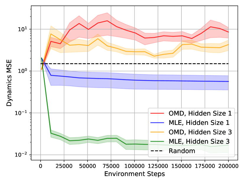
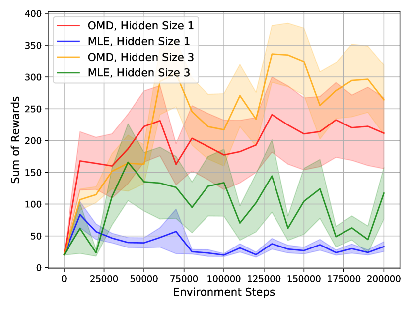
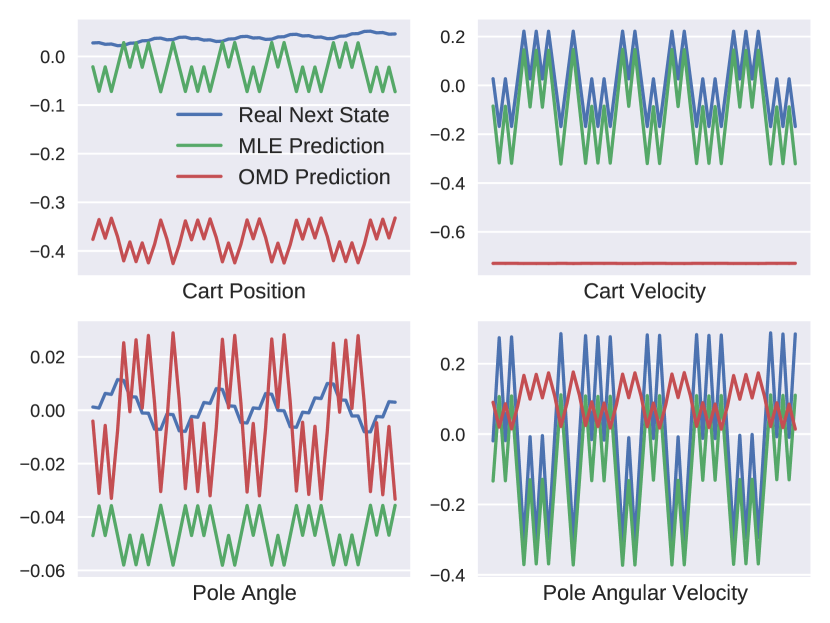
Likelihood of OMD model. We show the mean squared error (MSE) of OMD and MLE dynamics predictions in Figure 5. Quantitatively, the MSE of OMD models is higher than the MSE of a randomly initialized model, while OMD achieves higher returns than MLE. This finding suggests that the dynamics might not need to produce predictions close to the true states to be useful for planning.
Qualitatively, we visualize individual coordinates of the predictions under the model misspecification in Figure 5. We predict the immediate next states given a sequence of states and actions from an optimal trajectory. We use one of the runs of the OMD agent with the hidden size 1 that achieves optimal returns of 500 and observe that Cart Velocity predictions are nearly constant. On the other hand, an MLE model with the hidden size 1 spends its limited capacity to predict the fluctuations in Cart Velocity leading to a significant deterioration in obtained returns.
Overall, these findings suggest that the OMD agent achieves near-optimal returns, performs better than the MLE-based MBRL agent as well as VEP under model misspecification, and learns a model that is useful for control despite having low likelihood.
8 Discussion and Future Work
An exciting direction for future work is the extension of OMD to environments with image-based observations where model misspecification naturally arises. We expect that for complex visual domains, learning a control-oriented model should be more effective compared to model-based methods that rely on reconstruction [44, 34]. Based on Figure 5, we also conjecture that OMD can learn an abstract model that can ignore parts of the original state space that are irrelevant for control. This might allow applying OMD in a zero-shot manner for transfer learning tasks where the underlying dynamics remain unchanged.
Implicit differentiation is not the only way to solve the described constrained optimization problems. Other alternatives include using Lagrangian methods as proposed for the tabular case in [7]. Since extending the approach to non-tabular MDPs would require an additional approximator for Lagrange multipliers, we conjecture that finding a saddle point is going to be less stable than using the IFT.
9 Conclusion
The paper proposes optimal model design (OMD), a method for learning control-oriented models that addresses the shortcomings of likelihood-based MBRL approaches. OMD optimizes the expected returns in an end-to-end manner and alleviates the objective mismatch of standard MBRL methods that train models using a proxy of the true RL objective. Theoretically, we characterize the set of optimal solutions to OMD and illustrate the efficacy of OMD over MLE agents for approximating optimal value functions. Empirically, we introduce approximations to apply OMD to non-tabular environments and demonstrate the improved performance of OMD in settings with limited model capacity. Perhaps surprisingly, we find that the OMD model can have low likelihood, yet the model is useful for maximizing returns. Overall, OMD sheds light on the potential of control-oriented models for model-based reinforcement learning.
Acknowledgments and Disclosure of Funding
EN thanks Iurii Kemaev and Clement Gehring for invaluable help with JAX; Tristan Deleu, Gauthier Gidel, Amy Zhang, Aravind Rajeswaran, Ilya Kostrikov, Brandon Amos, and Aaron Courville for insightful discussions; Pierluca D’Oro, David Brandfonbrener, Valentin Thomas, and Timur Garipov for useful suggestions on the early draft of the paper; Compute Canada for providing computational resources. This work was partially supported by Facebook CIFAR AI Chair and IVADO.
References
- Abachi et al. [2020] Romina Abachi, Mohammad Ghavamzadeh, and Amir-massoud Farahmand. Policy-aware model learning for policy gradient methods. arXiv preprint arXiv:2003.00030, 2020.
- Abbad and Filar [1992] M. Abbad and J.A. Filar. Perturbation and stability theory for markov control problems. IEEE Transactions on Automatic Control, 37(9):1415–1420, 1992. doi: 10.1109/9.159584.
- Amos and Yarats [2020] Brandon Amos and Denis Yarats. The differentiable cross-entropy method. In International Conference on Machine Learning, pages 291–302. PMLR, 2020.
- Amos et al. [2018] Brandon Amos, Ivan Jimenez, Jacob Sacks, Byron Boots, and J Zico Kolter. Differentiable mpc for end-to-end planning and control. In Advances in Neural Information Processing Systems, pages 8289–8300, 2018.
- Ayoub et al. [2020] Alex Ayoub, Zeyu Jia, Csaba Szepesvari, Mengdi Wang, and Lin F Yang. Model-based reinforcement learning with value-targeted regression. arXiv preprint arXiv:2006.01107, 2020.
- Babuschkin et al. [2020] Igor Babuschkin, Kate Baumli, Alison Bell, Surya Bhupatiraju, Jake Bruce, Peter Buchlovsky, David Budden, Trevor Cai, Aidan Clark, Ivo Danihelka, Claudio Fantacci, Jonathan Godwin, Chris Jones, Tom Hennigan, Matteo Hessel, Steven Kapturowski, Thomas Keck, Iurii Kemaev, Michael King, Lena Martens, Vladimir Mikulik, Tamara Norman, John Quan, George Papamakarios, Roman Ring, Francisco Ruiz, Alvaro Sanchez, Rosalia Schneider, Eren Sezener, Stephen Spencer, Srivatsan Srinivasan, Wojciech Stokowiec, and Fabio Viola. The DeepMind JAX Ecosystem, 2020. URL http://github.com/deepmind.
- Bacon et al. [2019] Pierre-Luc Bacon, Florian Schäfer, Clement Gehring, Animashree Anandkumar, and Emma Brunskill. A lagrangian method for inverse problems in reinforcement learning. In Optimization in RL workshop at NeurIPS 2019, 2019.
- Bai et al. [2019] Shaojie Bai, J Zico Kolter, and Vladlen Koltun. Deep equilibrium models. In Advances in Neural Information Processing Systems, pages 690–701, 2019.
- Barto et al. [1983] Andrew G Barto, Richard S Sutton, and Charles W Anderson. Neuronlike adaptive elements that can solve difficult learning control problems. IEEE transactions on systems, man, and cybernetics, (5):834–846, 1983.
- Beattie et al. [2016] Charles Beattie, Joel Z Leibo, Denis Teplyashin, Tom Ward, Marcus Wainwright, Heinrich Küttler, Andrew Lefrancq, Simon Green, Víctor Valdés, Amir Sadik, et al. Deepmind lab. arXiv preprint arXiv:1612.03801, 2016.
- Bellemare et al. [2013] Marc G Bellemare, Yavar Naddaf, Joel Veness, and Michael Bowling. The arcade learning environment: An evaluation platform for general agents. Journal of Artificial Intelligence Research, 47:253–279, 2013.
- Boots et al. [2011] Byron Boots, Sajid M. Siddiqi, and Geoffrey J. Gordon. Closing the learning-planning loop with predictive state representations. Int. J. Robotics Res., 30(7):954–966, 2011. doi: 10.1177/0278364911404092.
- Borkar and Varaiya [1979] V. Borkar and P. Varaiya. Adaptive control of markov chains, i: Finite parameter set. IEEE Transactions on Automatic Control, 24(6):953–957, December 1979.
- Boyd et al. [2004] Stephen Boyd, Stephen P Boyd, and Lieven Vandenberghe. Convex optimization. Cambridge university press, 2004.
- Bradbury et al. [2018] James Bradbury, Roy Frostig, Peter Hawkins, Matthew James Johnson, Chris Leary, Dougal Maclaurin, George Necula, Adam Paszke, Jake VanderPlas, Skye Wanderman-Milne, and Qiao Zhang. JAX: composable transformations of Python+NumPy programs, 2018. URL http://github.com/google/jax.
- Christianson [1994] Bruce Christianson. Reverse accumulation and attractive fixed points. Optimization Methods and Software, 3(4):311–326, January 1994. doi: 10.1080/10556789408805572.
- Chua et al. [2018] Kurtland Chua, Roberto Calandra, Rowan McAllister, and Sergey Levine. Deep reinforcement learning in a handful of trials using probabilistic dynamics models. In Advances in Neural Information Processing Systems, pages 4754–4765, 2018.
- Dadashi et al. [2019] Robert Dadashi, Adrien Ali Taiga, Nicolas Le Roux, Dale Schuurmans, and Marc G Bellemare. The value function polytope in reinforcement learning. In International Conference on Machine Learning, pages 1486–1495. PMLR, 2019.
- Dauphin et al. [2014] Yann Dauphin, Razvan Pascanu, Caglar Gulcehre, Kyunghyun Cho, Surya Ganguli, and Yoshua Bengio. Identifying and attacking the saddle point problem in high-dimensional non-convex optimization. arXiv preprint arXiv:1406.2572, 2014.
- Denardo [1967] Eric V. Denardo. Contraction mappings in the theory underlying dynamic programming. SIAM Review, 9(2):165–177, April 1967. doi: 10.1137/1009030.
- Dorato et al. [1994] Peter Dorato, Vito Cerone, and Chaouki Abdallah. Linear-quadratic control: an introduction. Simon & Schuster, Inc., 1994.
- D’Oro et al. [2020] Pierluca D’Oro, Alberto Maria Metelli, Andrea Tirinzoni, Matteo Papini, and Marcello Restelli. Gradient-aware model-based policy search. In Proceedings of the AAAI Conference on Artificial Intelligence, volume 34, pages 3801–3808, 2020.
- Farahmand et al. [2017] Amir-massoud Farahmand, Andre Barreto, and Daniel Nikovski. Value-aware loss function for model-based reinforcement learning. In Artificial Intelligence and Statistics, pages 1486–1494, 2017.
- Finn et al. [2017] Chelsea Finn, Pieter Abbeel, and Sergey Levine. Model-agnostic meta-learning for fast adaptation of deep networks. In International Conference on Machine Learning, pages 1126–1135. PMLR, 2017.
- Fujimoto et al. [2018] Scott Fujimoto, Herke Hoof, and David Meger. Addressing function approximation error in actor-critic methods. In International Conference on Machine Learning, pages 1587–1596. PMLR, 2018.
- Gehring et al. [2019] Clement Gehring, Pierre-Luc Bacon, and Florian Schaefer. FAX: differentiating fixed point problems in JAX, 2019. Available at: https://github.com/gehring/fax.
- Georgin [1978] J. P. Georgin. Estimation et controle des chaines de markov sur des espaces arbitraires. In Lecture Notes in Mathematics, pages 71–113. Springer Berlin Heidelberg, 1978. doi: 10.1007/bfb0063261.
- Grefenstette et al. [1990] John J. Grefenstette, Connie Loggia Ramsey, and Alan C. Schultz. Learning sequential decision rules using simulation models and competition. Machine Learning, 5(4):355–381, October 1990. doi: 10.1007/bf00116876.
- Griewank and Walther [2008] Andreas Griewank and Andrea Walther. Evaluating Derivatives. Society for Industrial and Applied Mathematics, January 2008.
- Grimm et al. [2020] Christopher Grimm, André Barreto, Satinder Singh, and David Silver. The value equivalence principle for model-based reinforcement learning. Advances in Neural Information Processing Systems, 33, 2020.
- Haarnoja et al. [2018a] Tuomas Haarnoja, Aurick Zhou, Pieter Abbeel, and Sergey Levine. Soft actor-critic: Off-policy maximum entropy deep reinforcement learning with a stochastic actor. In International Conference on Machine Learning, pages 1861–1870. PMLR, 2018a.
- Haarnoja et al. [2018b] Tuomas Haarnoja, Aurick Zhou, Kristian Hartikainen, George Tucker, Sehoon Ha, Jie Tan, Vikash Kumar, Henry Zhu, Abhishek Gupta, Pieter Abbeel, et al. Soft actor-critic algorithms and applications. arXiv preprint arXiv:1812.05905, 2018b.
- Hafner et al. [2019] Danijar Hafner, Timothy Lillicrap, Ian Fischer, Ruben Villegas, David Ha, Honglak Lee, and James Davidson. Learning latent dynamics for planning from pixels. In International Conference on Machine Learning, pages 2555–2565. PMLR, 2019.
- Hafner et al. [2020] Danijar Hafner, Timothy Lillicrap, Mohammad Norouzi, and Jimmy Ba. Mastering atari with discrete world models. arXiv preprint arXiv:2010.02193, 2020.
- Hasselt [2010] Hado Hasselt. Double q-learning. Advances in neural information processing systems, 23:2613–2621, 2010.
- Heek et al. [2020] Jonathan Heek, Anselm Levskaya, Avital Oliver, Marvin Ritter, Bertrand Rondepierre, Andreas Steiner, and Marc van Zee. Flax: A neural network library and ecosystem for JAX, 2020. URL http://github.com/google/flax.
- Hernández-Lerma and Marcus [1985] O. Hernández-Lerma and S. I. Marcus. Adaptive control of discounted markov decision chains. Journal of Optimization Theory and Applications, 46(2):227–235, June 1985. doi: 10.1007/bf00938426.
- Hunter [2007] John D Hunter. Matplotlib: A 2d graphics environment. IEEE Annals of the History of Computing, 9(03):90–95, 2007.
- Iyengar [2005] Garud N. Iyengar. Robust dynamic programming. Mathematics of Operations Research, 30(2):257–280, May 2005. doi: 10.1287/moor.1040.0129.
- Janner et al. [2019] Michael Janner, Justin Fu, Marvin Zhang, and Sergey Levine. When to trust your model: Model-based policy optimization. In Advances in Neural Information Processing Systems, pages 12519–12530, 2019.
- Jiang [2018] Nan Jiang. Lecture notes on statistical reinforcement learning. 2018.
- Jones et al. [2014] Eric Jones, Travis Oliphant, and Pearu Peterson. SciPy: Open source scientific tools for Python. 2014.
- Joseph et al. [2013] Joshua Joseph, Alborz Geramifard, John W Roberts, Jonathan P How, and Nicholas Roy. Reinforcement learning with misspecified model classes. In 2013 IEEE International Conference on Robotics and Automation, pages 939–946. IEEE, 2013.
- Kaiser et al. [2019] Lukasz Kaiser, Mohammad Babaeizadeh, Piotr Milos, Blazej Osinski, Roy H Campbell, Konrad Czechowski, Dumitru Erhan, Chelsea Finn, Piotr Kozakowski, Sergey Levine, et al. Model-based reinforcement learning for atari. arXiv preprint arXiv:1903.00374, 2019.
- Kalashnikov et al. [2021] Dmitry Kalashnikov, Jacob Varley, Yevgen Chebotar, Benjamin Swanson, Rico Jonschkowski, Chelsea Finn, Sergey Levine, and Karol Hausman. Mt-opt: Continuous multi-task robotic reinforcement learning at scale. arXiv preprint arXiv:2104.08212, 2021.
- Kearns and Singh [2002] Michael Kearns and Satinder Singh. Near-optimal reinforcement learning in polynomial time. Machine learning, 49(2):209–232, 2002.
- Kluyver et al. [2016] Thomas Kluyver, Benjamin Ragan-Kelley, Fernando Pérez, Brian E Granger, Matthias Bussonnier, Jonathan Frederic, Kyle Kelley, Jessica B Hamrick, Jason Grout, Sylvain Corlay, et al. Jupyter Notebooks-a publishing format for reproducible computational workflows., volume 2016. 2016.
- Krantz and Parks [2012] Steven G Krantz and Harold R Parks. The implicit function theorem: history, theory, and applications. Springer Science & Business Media, 2012.
- Kurano [1972] Masami Kurano. Discrete-time markovian decision processes with an unknown parameter-average return criterion. Journal of the Operations Research Society of Japan, 15(2):67–76, 1972.
- Lambert et al. [2020] Nathan Lambert, Brandon Amos, Omry Yadan, and Roberto Calandra. Objective mismatch in model-based reinforcement learning. arXiv preprint arXiv:2002.04523, 2020.
- Levine [2018] Sergey Levine. Reinforcement learning and control as probabilistic inference: Tutorial and review. arXiv preprint arXiv:1805.00909, 2018.
- Li et al. [2006] Lihong Li, Thomas J Walsh, and Michael L Littman. Towards a unified theory of state abstraction for mdps. ISAIM, 4:5, 2006.
- Lin [1992] Long-Ji Lin. Self-improving reactive agents based on reinforcement learning, planning and teaching. Machine Learning, 8(3-4):293–321, May 1992. doi: 10.1007/bf00992699.
- Lorraine et al. [2020] Jonathan Lorraine, Paul Vicol, and David Duvenaud. Optimizing millions of hyperparameters by implicit differentiation. In International Conference on Artificial Intelligence and Statistics, pages 1540–1552. PMLR, 2020.
- Ludwig and Walters [1982] D. Ludwig and C.J. Walters. Optimal harvesting with imprecise parameter estimates. Ecological Modelling, 14(3-4):273–292, January 1982. doi: 10.1016/0304-3800(82)90023-0.
- Mandl [1974] P. Mandl. Estimation and control in markov chains. Advances in Applied Probability, 6(1):40–60, March 1974. doi: 10.2307/1426206.
- Manfred [1987] Schäl Manfred. Estimation and control in discounted stochastic dynamic programming. Stochastics, 20(1):51–71, January 1987. doi: 10.1080/17442508708833435.
- McKinney [2012] Wes McKinney. Python for data analysis: Data wrangling with Pandas, NumPy, and IPython. " O’Reilly Media, Inc.", 2012.
- Mnih et al. [2015] Volodymyr Mnih, Koray Kavukcuoglu, David Silver, Andrei A Rusu, Joel Veness, Marc G Bellemare, Alex Graves, Martin Riedmiller, Andreas K Fidjeland, Georg Ostrovski, et al. Human-level control through deep reinforcement learning. nature, 518(7540):529–533, 2015.
- Nair and Hinton [2010] Vinod Nair and Geoffrey E Hinton. Rectified linear units improve restricted boltzmann machines. In Icml, 2010.
- Nilim and Ghaoui [2005] Arnab Nilim and Laurent El Ghaoui. Robust control of markov decision processes with uncertain transition matrices. Operations Research, 53(5):780–798, October 2005. doi: 10.1287/opre.1050.0216.
- Oliphant [2006] Travis E Oliphant. A guide to NumPy, volume 1. Trelgol Publishing USA, 2006.
- Oliphant [2007] Travis E Oliphant. Python for scientific computing. Computing in Science & Engineering, 9(3):10–20, 2007.
- Rajeswaran et al. [2019] Aravind Rajeswaran, Chelsea Finn, Sham M Kakade, and Sergey Levine. Meta-learning with implicit gradients. In Advances in Neural Information Processing Systems, pages 113–124, 2019.
- Rajeswaran et al. [2020] Aravind Rajeswaran, Igor Mordatch, and Vikash Kumar. A game theoretic framework for model based reinforcement learning. arXiv preprint arXiv:2004.07804, 2020.
- Rubinstein [1997] Reuven Y Rubinstein. Optimization of computer simulation models with rare events. European Journal of Operational Research, 99(1):89–112, 1997.
- Rust [1988] John Rust. Maximum likelihood estimation of discrete control processes. SIAM journal on control and optimization, 26(5):1006–1024, 1988.
- Sagun et al. [2017] Levent Sagun, Utku Evci, V Ugur Guney, Yann Dauphin, and Leon Bottou. Empirical analysis of the hessian of over-parametrized neural networks. arXiv preprint arXiv:1706.04454, 2017.
- Sato et al. [1988] M. Sato, K. Abe, and H. Takeda. Learning control of finite markov chains with an explicit trade-off between estimation and control. IEEE Transactions on Systems, Man, and Cybernetics, 18(5):677–684, 1988. doi: 10.1109/21.21595.
- Schrittwieser et al. [2019] Julian Schrittwieser, Ioannis Antonoglou, Thomas Hubert, Karen Simonyan, Laurent Sifre, Simon Schmitt, Arthur Guez, Edward Lockhart, Demis Hassabis, Thore Graepel, et al. Mastering atari, go, chess and shogi by planning with a learned model. arXiv preprint arXiv:1911.08265, 2019.
- Skelton [1989] RE Skelton. Model error concepts in control design. International Journal of Control, 49(5):1725–1753, 1989.
- Sorg et al. [2010] Jonathan Sorg, Richard L Lewis, and Satinder Singh. Reward design via online gradient ascent. In J. Lafferty, C. Williams, J. Shawe-Taylor, R. Zemel, and A. Culotta, editors, Advances in Neural Information Processing Systems, volume 23, pages 2190–2198. Curran Associates, Inc., 2010.
- Sutton [1991] Richard S Sutton. Dyna, an integrated architecture for learning, planning, and reacting. ACM Sigart Bulletin, 2(4):160–163, 1991.
- Sutton and Barto [2018] Richard S Sutton and Andrew G Barto. Reinforcement learning: An introduction. MIT press, 2018.
- Sutton et al. [1999] Richard S Sutton, David McAllester, Satinder Singh, and Yishay Mansour. Policy gradient methods for reinforcement learning with function approximation. Advances in neural information processing systems, 12:1057–1063, 1999.
- Tamar et al. [2016] Aviv Tamar, Yi Wu, Garrett Thomas, Sergey Levine, and Pieter Abbeel. Value iteration networks. arXiv preprint arXiv:1602.02867, 2016.
- Theil [1957] H. Theil. A note on certainty equivalence in dynamic planning. Econometrica, 25(2):346, April 1957.
- Todorov et al. [2012] Emanuel Todorov, Tom Erez, and Yuval Tassa. Mujoco: A physics engine for model-based control. In 2012 IEEE/RSJ International Conference on Intelligent Robots and Systems, pages 5026–5033. IEEE, 2012.
- Van Der Walt et al. [2011] Stefan Van Der Walt, S Chris Colbert, and Gael Varoquaux. The numpy array: a structure for efficient numerical computation. Computing in science & engineering, 13(2):22–30, 2011.
- Van Rossum and Drake Jr [1995] Guido Van Rossum and Fred L Drake Jr. Python tutorial, volume 620. Centrum voor Wiskunde en Informatica Amsterdam, 1995.
- Watkins and Dayan [1992] Christopher JCH Watkins and Peter Dayan. Q-learning. Machine learning, 8(3-4):279–292, 1992.
- Xu and Mannor [2010] Huan Xu and Shie Mannor. Distributionally robust markov decision processes. In J. Lafferty, C. Williams, J. Shawe-Taylor, R. Zemel, and A. Culotta, editors, Advances in Neural Information Processing Systems, volume 23, pages 2505–2513. Curran Associates, Inc., 2010.
- Yu et al. [2020] Tianhe Yu, Garrett Thomas, Lantao Yu, Stefano Ermon, James Zou, Sergey Levine, Chelsea Finn, and Tengyu Ma. Mopo: Model-based offline policy optimization. In Advances in Neural Information Processing Systems 33 pre-proceedings, 2020.
- Ziebart et al. [2008] Brian D Ziebart, Andrew L Maas, J Andrew Bagnell, and Anind K Dey. Maximum entropy inverse reinforcement learning. In Aaai, volume 8, pages 1433–1438. Chicago, IL, USA, 2008.
Supplementary Material
Appendix A Implicit Differentiation in JAX
We provide an implementation of implicit differentiation in JAX [6, 36] by adapting the code from the library for finding fixed points [26]. The implementation requires a solver that takes parameters and an initial as input and outputs such that . Then, we define a custom vector-Jacobian product that allows using as a block in a differentiable computational graph. We highlight the importance of having an implementation without explicitly forming the matrices in (7) which is crucial for large-scale applications. The implementation allows using both the version with the inverse Jacobian term as well as with the identity approximation as discussed in Section 6.
The implicit function theorem (IFT), which we prove in the next appendix, allows differentiating outputs of black-box functions that do not have a closed (differentiable) form. For example, in Section 4.2, function takes as input the parameters of the model and applies fixed-point iteration until convergence to find the optimal value function for the given parameters. This contrasts implicit differentiation to other meta-learning algorithms like MAML [24] that differentiate through the iterations of the inner loop procedure.
Appendix B Proof of IFT
Proof.
By the assumption, we have
Taking the total derivative of with respect to , we have
Rearranging the terms and using the invertibility of the Jacobian, we get
∎
Appendix C Sensitivity to IFT Approximations
The IFT provides a way to calculate the derivatives of a black-box function . The expression (7) is valid under the assumptions that
-
1.
the inner loop solution satisfies the equation exactly;
-
2.
the Jacobian term is inverted accurately.
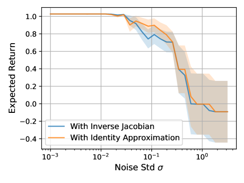
Ensuring both of the conditions can be challenging for large-scale applications. This appendix analyzes the sensitivity to the conditions in a controlled manner for the 2-state MDP from Figure 3, while Appendix E studies the sensitivity for the function approximation case. At every outer loop iteration, we calculate the exact , add gaussian noise with standard deviation , and observe the effect on the expected returns after the convergence of . Figure 6 demonstrates the results for the exact outer loop gradient as well as the gradient using the identity approximation of the inverse Jacobian term. Surprisingly, we did not observe significant benefits of using the Jacobian . We conjecture that the inverse Jacobian acts like a preconditioner [14] on and the preconditioner is useful in our setting only near the exact inner loop solutions . We leave the theoretical investigation of the IFT sensitivity as future work and refer the reader to Lorraine et al. [54] for a discussion about approximations of the Jacobian term.
Appendix D Experimental Details
In Section 7, we use CartPole [9], an environment with 2 actions, 4-dimensional continuous state space, and optimal returns of 500. We train the agents for 200000 environment steps. The temperature is 0.01. We sample from the replay buffer with a mini-batch size of 256. The discount factor is 0.99. At each time step during training, the agent chooses a random action with a probability of 0.1 for exploration. We have a separate copy of the environment where we evaluate the agent and take the average over 10 runs to estimate the returns. We run each experiment using 10 random seeds.
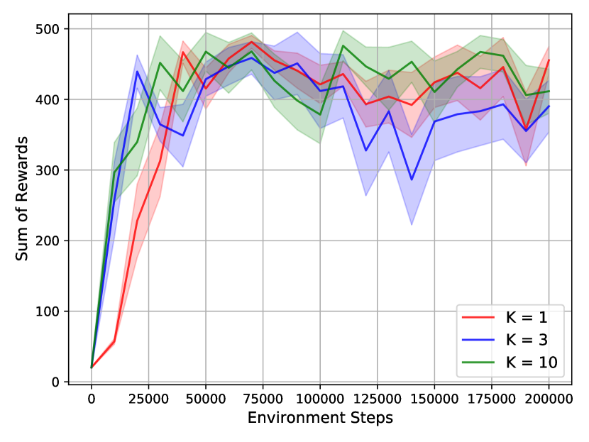
We set the number of Q-function updates equal to 1. For the results with and , see Figure 7. We highlight that after each outer loop step, weights are warm-started using the last iterate of the previous inner loop (instead of randomly initializing and training from scratch). We use Adam optimizer with the learning rate for updating and perform a hyperparameter sweep over the learning rate for in . We make a sweep over the moving average coefficient for the target network in . Both of the parameters control how fast the Q-network parameters are updated relatively to the model parameters. Since the CartPole environment is non-stochastic, we use a deterministic dynamics model. All networks have two hidden layers and ReLU activations [60]. For both hidden layers in all networks, we set the dimensionality to 32. In the experiment with the limited model class capacity, we vary the hidden dimensionality in for the dynamics and reward networks to measure how the limitation affects the agent’s performance. In the experiment with the distractors, we vary the number of gaussians in to measure how the uninformative state components affect the returns.
For the value equivalence principle (VEP) baseline, we have followed the experimental setup from the original paper [30]. Perhaps surprisingly, the authors find that it suffices to use a set of all deterministic state-independent policies as and 5 random value functions as for CartPole (see Appendix A.2.3 in [30]).
We have used CPU-only nodes of the internal cluster. Each experiment requires 10 seeds 3 algorithms 2 ’s 6 hidden sizes / 6 numbers of distractors 3 LRs resulting in 2160 total jobs.
Appendix E Ablation Study
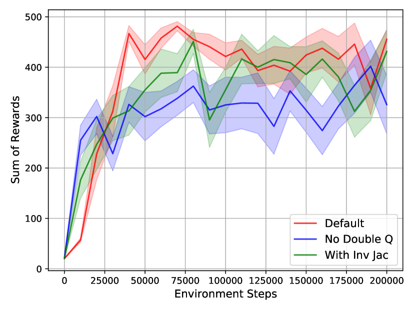
Section 6 introduces a series of approximations to scale the OMD algorithm to non-tabular environments. We analyze the effect of the approximations by varying the number of inner loop steps , using the inverse Jacobian term, and using a single Q-function estimator (without double Q-learning). Figure 7 summarizes the findings of the ablations. We did not observe significant changes in performance for different values of for CartPole. The result suggests that as long as the Q-network update speed (which is also controlled by the target update coefficient and learning rates) stays aligned with the model update speed, adding more inner loop steps is not necessary.
We observed that Q-functions trained with OMD can be prone to overestimation of Q-values showing that double Q-learning is important for OMD. We conjecture that training a model that maximizes the returns can amplify the overestimation bias [35] caused by using (soft) maximized sampled targets.
Surprisingly, we did not observe significant benefits from using the inverse Jacobian . We conjecture that there are two reasons explaining the phenomenon. First, the modified constraint in (12) forces the gradient of to be zero, implying that the Jacobian is in fact the Hessian matrix . Dauphin et al. [19], Sagun et al. [68] observed that Hessians of neural networks tend to be singular. Since a system of linear equations with a singular matrix has multiple solutions, it is up to a linear algebra solver to choose the solution. One of the alternatives would be a min-norm solution corresponding to the Moore-Penrose pseudoinverse and the solution might not be providing a useful inductive bias for the learning process of . Second, the Jacobian term could be useful only in proximity to the exact inner loop solution . Since the practical algorithm performs only inner loop steps and does not reach the exact , the curvature information provided by the Jacobian might not be beneficial for training .
Finally, we tried to use the gradient constraint in (12) in the tabular setting. We got similar results as with the constraint on Q-values in (2) suggesting that the two constraints have similar effects on the learning process. Overall, the ablation study provides evidence that OMD is robust to the choice of the number of inner loop steps and the IFT approximations, while double Q-learning is the only important algorithmic modification.
Appendix F Results on HalfCheetah
We provide an additional comparison of OMD and MLE agents under the model misspecification on MuJoCo HalfCheetah [78]. For both agents, the inner optimizer is Soft Actor-Critic (SAC) [31, 32] with the default configuration. OMD trains the model using 13. The MLE agent trains the model with MSE effectively becoming the MBPO algorithm [40] without having an ensemble of models and learning the variance of the predictions.
We perform a hyperparameter sweep over the model learning rate in , over the SAC networks learning rate in , and over in . Model hidden size is 64 for the experiment with distractors.
Figure 8 summarizes the results. Similarly to the observations on the tabular and CartPole environments, the experiments provide evidence that OMD should be preferred over the likelihood-based agent in the model misspecification setup.
Appendix G Proof of Bounds
Section 5.2 discusses the bounds on approximation error obtained by the MLE and OMD agents. We first prove a lemma relating the error of the model approximation and the Bellman operator approximation. We then prove a theorem giving a bound on error. For simplicity, we focus on the case with the Bellman error in the true MDP (6) as the objective function and “hard” versions of the Bellman optimality operators which are obtained by taking the limit of the log-sum-exp temperature . Note that results for MLE hold for any agent that approximates the reward and dynamics functions, but we call the agent MLE since it is a common choice for model parameters estimation.
Notation. We denote and as vectors of transition probabilities and Q-values for all states in . The MLE model is given by and the corresponding Bellman optimality operator is denoted as . To have a distinction between OMD and MLE, we denote OMD parameters as and the corresponding operator as . is the infinity norm of a function . is a vector of an appropriate size with ones as entries.
Lemma 1.
(Bellman operator error bound) Let be an action-value function. If the dynamics and the reward have the bounded errors and , and the reward function is bounded , we have
| (15) |
Proof.
Using the derivations similar to the proof of the simulation lemma [41], we obtain for any state-action pair
Since the inequalities hold for all state-action pairs, we can take the maximum over and obtain
∎
See 2
Proof.
(OMD) For all state-action pairs we get
Taking the maximum over , we get the recursion:
(MLE) The proof for MLE can be obtained using the same derivations and additionally using the result of the lemma bounding the difference between the Bellman operators:
∎
The last inequality demonstrates that the OMD bound is tighter. OMD model directly optimizes , while MLE minimizes and that only upper bound as suggested by the lemma. Hence, given the same budget of representational capacity, OMD will learn a model that is more helpful for approximating the optimal Q-function. Finally, Figure 3 empirically supports our theoretical findings showing that both the approximation error and the error-bound gap are smaller for OMD.