Signatured Deep Fictitious Play for Mean Field Games with Common Noise

Ming Min    Ruimeng Hu
Abstract

Existing deep learning methods for solving mean-field games (MFGs) with common noise fix the sampling common noise paths and then solve the corresponding MFGs. This leads to a nested-loop structure with millions of simulations of common noise paths in order to produce accurate solutions, which results in prohibitive computational cost and limits the applications to a large extent. In this paper, based on the rough path theory, we propose a novel single-loop algorithm, named signatured deep fictitious play, by which we can work with the unfixed common noise setup to avoid the nested-loop structure and reduce the computational complexity significantly. The proposed algorithm can accurately capture the effect of common uncertainty changes on mean-field equilibria without further training of neural networks, as previously needed in the existing machine learning algorithms. The efficiency is supported by three applications, including linear-quadratic MFGs, mean-field portfolio game, and mean-field game of optimal consumption and investment. Overall, we provide a new point of view from the rough path theory to solve MFGs with common noise with significantly improved efficiency and an extensive range of applications. In addition, we report the first deep learning work to deal with extended MFGs (a mean-field interaction via both the states and controls) with common noise.

Mean field games with common noise, rough path theory, signature, deep fictitious play

1 Introduction

Stochastic differential games study the strategic interaction of rational decision-makers in an uncertain dynamical system, and have been widely applied to many areas, including social science, system science, and computer science. For realistic models, the problem usually lacks tractability and needs numerical methods. With a large number of players resulting in high-dimensional problems, conventional algorithms soon lose efficiency and one may resort to recently developed machine learning tools (Hu, 2021; Han & Hu, 2020; Han etΒ al., 2020). On the other hand, one could utilize its limiting mean-field version, mean-field games (MFGs), to approximate the n𝑛n-player game for large n𝑛n (e.g., Han etΒ al. (2021)). Introduced independently in Huang etΒ al. (2006); Lasry & Lions (2007), MFGs study the decision making problem of a continuum of agents, aiming to provide asymptotic analysis of the finite player model in which players interact through their empirical distribution. In an MFG, each agent is infinitesimal, whose decision can not affect the population law. Therefore, the problem can be solved by focusing on the optimal decision of a representative agent in response to the average behavior of the entire population and a fixed-point problem (cf. equation (2.5)). The MFG model has inspired tremendous applications, not only in finance and economics, such as system risk (Carmona etΒ al., 2015), high-frequency trading (Lachapelle etΒ al., 2016) and crowd trading (Cardaliaguet & Lehalle, 2018), but also to population dynamics (Achdou etΒ al., 2017; Djehiche etΒ al., 2017; Achdou & Lasry, 2019) and sanitary vaccination (Hubert & Turinici, 2018; Elie etΒ al., 2020a), to list a few. For a systematical introduction of MFGs, see Caines etΒ al. (2017); Carmona & Delarue (2018a, b).

In MFGs, the random shocks to the dynamical system can be from two sources: idiosyncratic to the individual players and common to all players, i.e., decision-makers face correlated randomness. While MFGs were initially introduced with only idiosyncratic noise as seen in most of the literature, games with common noise, referred to as MFGs with common noise, have attracted significant attention recently (Lacker & Webster, 2015; Carmona etΒ al., 2016; Ahuja, 2016; Graber, 2016). The inclusion of common noise is natural in many contexts, such as multi-agent trading in a common stock market, or systemic risk induced through inter-bank lending/borrowing. In reality, players make decisions in a common environment (e.g., trade in the same stock market). Therefore, their states are subject to correlated random shocks, which can be modeled by individual noises and a common noise. In this modeling, observing the state dynamics will be sufficient, and one does not need to observe the noises. These applications make it crucial to develop efficient and accurate algorithms for computing MFGs with common noise.

Theoretically, MFGs with common noise can be formulated as an infinite-dimensional master equation, which is the type of second-order nonlinear Hamilton-Jacobi-Bellman equation involving derivatives with respect to a probability measure. Therefore, direct simulation is infeasible due to the difficulty of discretizing the probability space. An alternative way of solving MFGs with common noise is to formulate it into a stochastic Fokker-Planck/Hamilton-Jacobi-Bellman system, which has a complicated form with common noise, forward-backward coupling, and second-order differential operators. The third kind of approaches turns it into forward backward stochastic differential equations (FBSDE) of McKean-Vlasov type (cf. Carmona & Delarue (2018b, Chapter 2)), which in general requires convexity of the Hamiltonian. For all three approaches, the common assumption is the monotonicity condition that ensures uniqueness. Regarding simulation, existing deep learning methods fix the sampling common noise paths and then solve the corresponding MFGs, which leads to a nested-loop structure with millions of simulations of common noise paths to produce accurate predictions for unseen common shock realizations. Then the computational cost becomes prohibitive and limits the applications to a large extent.

In this paper, we solve MFGs with common noise by directly parameterizing the optimal control using deep neural networks in spirit of (Han & E, 2016), and conducting a global optimization. We integrate the signature from rough path theory, and fictitious play from game theory for efficiency and accuracy, and term the algorithm Signatured Deep Fictitious Play (Sig-DFP). The proposed algorithm avoids solving the three aforementioned complicated equations (master equation, Stochastic FP/HJB, FBSDE) and does not have uniqueness issues.

Contribution. We design a novel efficient single-loop deep learning algorithm, Sig-DFP, for solving MFGs with common noise by integrating fictitious play (Brown, 1949) and Signature (Lyons etΒ al., 2007) from rough path theory. To our best knowledge, this is the first work focusing on the common noise setting, which can address heterogeneous MFGs and heterogeneous extended MFGs, both with common noise.

We prove that the Sig-DFP algorithm can reach mean-field equilibria as both the depth M𝑀M of the truncated signature and the stage n𝑛n of the fictitious play approaching infinity, subject to the universal approximation of neural networks. We demonstrate its convergence superiority on three benchmark examples, including homogeneous MFGs, heterogeneous MFGs, and heterogeneous extended MFGs, all with common noise, and with assumptions even beyond the technical requirements in the theorems. Moreover, the algorithm has the following advantages:

1. Temporal and spacial complexity are π’ͺ​(N​L​p+N​p2)π’ͺ𝑁𝐿𝑝𝑁superscript𝑝2\mathcal{O}(NLp+Np^{2}) and π’ͺ​(N​L​p)π’ͺ𝑁𝐿𝑝\mathcal{O}(NLp), compared to π’ͺ​(N2​L)π’ͺsuperscript𝑁2𝐿\mathcal{O}(N^{2}L) (for both time and space) in existing machine learning algorithms, with N𝑁N as the sample size, L𝐿L as the time discretization size, p=π’ͺ​(n0M)𝑝π’ͺsuperscriptsubscript𝑛0𝑀p=\mathcal{O}(n_{0}^{M}), n0subscript𝑛0n_{0} as the dimension of common noise.

2. Easy to apply the fictitious play strategy: only need to average over linear functionals with π’ͺ​(1)π’ͺ1\mathcal{O}(1) complexity.

Related Literature. After MFGs firstly introduced by Huang etΒ al. (2006) and Lasry & Lions (2007) under the setting of a continuum of homogeneous players but without common noise, it has been extended to many applicable settings, e.g., heterogeneous players games (Lacker & Zariphopoulou, 2019; Lacker & Soret, 2020) and major-minor players games (Huang, 2010; Nourian & Caines, 2013; Carmona & Zhu, 2016). A recent line of work studies MFGs with common noise (Carmona etΒ al., 2015; Bensoussan etΒ al., 2015; Ahuja, 2016; Cardaliaguet etΒ al., 2019). Despite its theoretical progress and importance for applications, efficient numerical algorithms focusing on common noise settings are still missing. Our work will fill this gap by integrating machine learning tools with learning procedures from game theory and signature from rough path theory.

Fictitious play was firstly proposed in Brown (1949, 1951) for normal-form games, as a learning procedure for finding Nash equilibria. It has been widely used in the Economic literature, and adapted to MFGs (Cardaliaguet & Hadikhanloo, 2017; Briani & Cardaliaguet, 2018) and finite-player stochastic differential games (Hu, 2021; Han & Hu, 2020; Han etΒ al., 2020; Xuan etΒ al., 2021).

Using machine learning to solve MFGs has also been considered, for both model-based setting (Carmona & Laurière, 2019; Ruthotto et al., 2020; Lin et al., 2020) and model-free reinforcement learning setting (Guo et al., 2019; Tiwari et al., 2019; Angiuli et al., 2020; Elie et al., 2020b), most of which did not consider common noise. Existing machine learning methods for MFGs with common noise were studied in Perrin et al. (2020), which have a nested-loop structure and require millions of simulations of common noise paths to produce accurate predictions for unseen common shock realizations.

The signature in rough path theory has been recently applied to machine learning as a feature map for sequential data. For example, KirΓ‘ly & Oberhauser (2019); Bonnier etΒ al. (2019); Toth & Oberhauser (2020); Min & Ichiba (2020) have used signatures in natural language processing, time series, and handwriting recognition, and Chevyrev & Oberhauser (2018); Ni etΒ al. (2020) studied the relation between signatures and distributions of sequential data. We refer to Lyons & Qian (2002); Lyons etΒ al. (2007) for a more detailed introduction of the signature and rough path theory.

2 Mean Field Games with Common Noise

We first introduce the following notations to precisely define MFGs with common noise. For a fixed time horizon T𝑇T, let (Wt)0≀t≀Tsubscriptsubscriptπ‘Šπ‘‘0𝑑𝑇(W_{t})_{0\leq t\leq T} and (Bt)0≀t≀Tsubscriptsubscript𝐡𝑑0𝑑𝑇(B_{t})_{0\leq t\leq T} be independent n𝑛n- and n0subscript𝑛0n_{0}-dimensional Brownian motions defined on a complete filtered probability space (Ξ©,β„±,𝔽={β„±t}0≀t≀T,β„™)formulae-sequenceΩℱ𝔽subscriptsubscriptℱ𝑑0𝑑𝑇ℙ(\Omega,\mathcal{F},\mathbb{F}=\{\mathcal{F}_{t}\}_{0\leq t\leq T},\mathbb{P}). We shall refer Wπ‘ŠW as the idiosyncratic noise and B𝐡B as the common noise of the system. Let β„±tBsubscriptsuperscriptℱ𝐡𝑑\mathcal{F}^{B}_{t} be the filtration generated by (Bt)0≀t≀Tsubscriptsubscript𝐡𝑑0𝑑𝑇(B_{t})_{0\leq t\leq T}, and 𝒫p​(ℝd)superscript𝒫𝑝superscriptℝ𝑑\mathcal{P}^{p}(\mathbb{R}^{d}) be the collection of probability measures on ℝdsuperscriptℝ𝑑\mathbb{R}^{d} with finite pt​hsuperscriptπ‘π‘‘β„Žp^{th} moment, i.e., ΞΌβˆˆπ’«p​(ℝd)πœ‡superscript𝒫𝑝superscriptℝ𝑑\mu\in\mathcal{P}^{p}(\mathbb{R}^{d}) if

(βˆ«β„dβ€–xβ€–p​dμ​(x))1/p<∞.superscriptsubscriptsuperscriptℝ𝑑superscriptnormπ‘₯𝑝differential-dπœ‡π‘₯1𝑝\left(\int_{\mathbb{R}^{d}}\|x\|^{p}\,\mathrm{d}\mu(x)\right)^{1/p}<\infty. (2.1)

We denote by ℳ​([0,T];𝒫2​(ℝd))β„³0𝑇superscript𝒫2superscriptℝ𝑑\mathcal{M}([0,T];\mathcal{P}^{2}(\mathbb{R}^{d})) the space of continuous β„±Bsuperscriptℱ𝐡\mathcal{F}^{B}-adapted stochastic flow of probability measures with the finite second moment, and by β„‹2​([0,T];ℝm)superscriptβ„‹20𝑇superscriptβ„π‘š\mathcal{H}^{2}([0,T];\mathbb{R}^{m}) the set of all β„±β„±\mathcal{F}-progressively measurable ℝmsuperscriptβ„π‘š\mathbb{R}^{m}-valued square-integrable processes.

Next, we introduce the concept of MFGs with common noise. Given an initial distribution ΞΌ0βˆˆπ’«2​(ℝd)subscriptπœ‡0superscript𝒫2superscriptℝ𝑑\mu_{0}\in\mathcal{P}^{2}(\mathbb{R}^{d}), and a stochastic flow of probability measures ΞΌ=(ΞΌt)0≀t≀Tβˆˆβ„³β€‹([0,T];𝒫2​(ℝd))πœ‡subscriptsubscriptπœ‡π‘‘0𝑑𝑇ℳ0𝑇superscript𝒫2superscriptℝ𝑑\mu=(\mu_{t})_{0\leq t\leq T}\in\mathcal{M}([0,T];\mathcal{P}^{2}(\mathbb{R}^{d})), we consider the stochastic control

inf(Ξ±t)0≀t≀T𝔼​[∫0Tf​(t,Xt,ΞΌt,Ξ±t)​dt+g​(XT,ΞΌT)],subscriptinfimumsubscriptsubscript𝛼𝑑0𝑑𝑇𝔼delimited-[]superscriptsubscript0𝑇𝑓𝑑subscript𝑋𝑑subscriptπœ‡π‘‘subscript𝛼𝑑differential-d𝑑𝑔subscript𝑋𝑇subscriptπœ‡π‘‡\displaystyle\inf_{(\alpha_{t})_{0\leq t\leq T}}\mathbb{E}[\int_{0}^{T}f(t,X_{t},\mu_{t},\alpha_{t})\,\mathrm{d}t+g(X_{T},\mu_{T})], (2.2)
where ​d​Xt=b​(t,Xt,ΞΌt,Ξ±t)​d​t+σ​(t,Xt,ΞΌt,Ξ±t)​d​WtwhereΒ dsubscript𝑋𝑑𝑏𝑑subscript𝑋𝑑subscriptπœ‡π‘‘subscript𝛼𝑑dπ‘‘πœŽπ‘‘subscript𝑋𝑑subscriptπœ‡π‘‘subscript𝛼𝑑dsubscriptπ‘Šπ‘‘\displaystyle\text{where }\,\mathrm{d}X_{t}=b(t,X_{t},\mu_{t},\alpha_{t})\,\mathrm{d}t+\sigma(t,X_{t},\mu_{t},\alpha_{t})\,\mathrm{d}W_{t}
+Οƒ0​(t,Xt,ΞΌt,Ξ±t)​d​Bt,superscript𝜎0𝑑subscript𝑋𝑑subscriptπœ‡π‘‘subscript𝛼𝑑dsubscript𝐡𝑑\displaystyle\hskip 55.00008pt+\sigma^{0}(t,X_{t},\mu_{t},\alpha_{t})\,\mathrm{d}B_{t}, (2.3)

with X0∼μ0similar-tosubscript𝑋0subscriptπœ‡0X_{0}\sim\mu_{0}. Here the representative agent controls his dynamics Xtsubscript𝑋𝑑X_{t} through a ℝmsuperscriptβ„π‘š\mathbb{R}^{m}-dimensional control process Ξ±tsubscript𝛼𝑑\alpha_{t}, and the drift coefficient b𝑏b, diffusion coefficients ΟƒπœŽ\sigma and Οƒ0superscript𝜎0\sigma^{0}, running cost f𝑓f and terminal cost g𝑔g are all measurable functions, with (b,Οƒ,Οƒ0,f):[0,T]×ℝd×𝒫2​(ℝd)×ℝm→ℝd×ℝdΓ—n×ℝdΓ—n0×ℝ:π‘πœŽsuperscript𝜎0𝑓→0𝑇superscriptℝ𝑑superscript𝒫2superscriptℝ𝑑superscriptβ„π‘šsuperscriptℝ𝑑superscriptℝ𝑑𝑛superscriptℝ𝑑subscript𝑛0ℝ(b,\sigma,\sigma^{0},f):[0,T]\times\mathbb{R}^{d}\times\mathcal{P}^{2}(\mathbb{R}^{d})\times\mathbb{R}^{m}\to\mathbb{R}^{d}\times\mathbb{R}^{d\times n}\times\mathbb{R}^{d\times n_{0}}\times\mathbb{R}, and g:ℝd×𝒫2​(ℝd)→ℝ:𝑔→superscriptℝ𝑑superscript𝒫2superscriptℝ𝑑ℝg:\mathbb{R}^{d}\times\mathcal{P}^{2}(\mathbb{R}^{d})\to\mathbb{R}.

Note that since ΞΌπœ‡\mu is stochastic, (2.2)–(2.3) is a control problem with random coefficients.

Definition 2.1 (Mean-field equilibrium).

The control-distribution flow pair Ξ±βˆ—=(Ξ±tβˆ—)0≀t≀Tβˆˆβ„‹2​([0,T];ℝm)superscriptπ›Όβˆ—subscriptsubscriptsuperscriptπ›Όβˆ—π‘‘0𝑑𝑇superscriptβ„‹20𝑇superscriptβ„π‘š\alpha^{\ast}=(\alpha^{\ast}_{t})_{0\leq t\leq T}\in\mathcal{H}^{2}([0,T];\mathbb{R}^{m}), ΞΌβˆ—βˆˆβ„³β€‹([0,T];𝒫2​(ℝd))superscriptπœ‡βˆ—β„³0𝑇superscript𝒫2superscriptℝ𝑑\mu^{\ast}\in\mathcal{M}([0,T];\mathcal{P}^{2}(\mathbb{R}^{d})) is a mean-field equilibrium to the MFG with common noise, if Ξ±βˆ—superscriptπ›Όβˆ—\alpha^{\ast} solves (2.2) given the stochastic measure flow ΞΌβˆ—superscriptπœ‡βˆ—\mu^{\ast}, and the conditional marginal distribution of the optimal path XtΞ±βˆ—superscriptsubscript𝑋𝑑superscriptπ›Όβˆ—X_{t}^{\alpha^{\ast}} given the common noise B𝐡B coincides with the measure flow ΞΌβˆ—superscriptπœ‡βˆ—\mu^{\ast}:

ΞΌtβˆ—=ℒ​(XtΞ±βˆ—|β„±tB),superscriptsubscriptπœ‡π‘‘βˆ—β„’conditionalsuperscriptsubscript𝑋𝑑superscriptπ›Όβˆ—superscriptsubscriptℱ𝑑𝐡\mu_{t}^{\ast}=\mathcal{L}(X_{t}^{\alpha^{\ast}}|\mathcal{F}_{t}^{B}), (2.4)

where β„’(β‹…|β„±)\mathcal{L}(\cdot|\mathcal{F}) is the conditional law given a filtration β„±β„±\mathcal{F}.

We remark that, with a continuum of agents, the measure ΞΌβˆ—superscriptπœ‡βˆ—\mu^{\ast} is not affected by a single agent’s choice, and the MFG is a standard control problem plus an additional fixed-point problem. More precisely, denote by Ξ±^ΞΌsuperscript^π›Όπœ‡\hat{\alpha}^{\mu} the optimal control of (2.2)–(2.3) given the stochastic measure flow ΞΌβˆˆβ„³β€‹([0,T];𝒫2​(ℝd))πœ‡β„³0𝑇superscript𝒫2superscriptℝ𝑑\mu\in\mathcal{M}([0,T];\mathcal{P}^{2}(\mathbb{R}^{d})), then ΞΌβˆ—superscriptπœ‡βˆ—\mu^{\ast} is a fixed point of

ΞΌt=ℒ​(XtΞ±^ΞΌ|β„±tB).subscriptπœ‡π‘‘β„’conditionalsuperscriptsubscript𝑋𝑑superscript^π›Όπœ‡superscriptsubscriptℱ𝑑𝐡\mu_{t}=\mathcal{L}(X_{t}^{\hat{\alpha}^{\mu}}|\mathcal{F}_{t}^{B}). (2.5)

MFGs without common noise: Note that with Οƒ0≑0superscript𝜎00\sigma^{0}\equiv 0, (2.2)–(2.3) is a MFG without common noise, and the flow of measures ΞΌtsubscriptπœ‡π‘‘\mu_{t} becomes deterministic.

Extended MFGs: In extended mean field games, the interactions between the representative agent and the population happen via both the states and controls, thus the functions (b,Οƒ,Οƒ0,f,g)π‘πœŽsuperscript𝜎0𝑓𝑔(b,\sigma,\sigma^{0},f,g) can also depend on ℒ​(Ξ±t|β„±tB)β„’conditionalsubscript𝛼𝑑superscriptsubscriptℱ𝑑𝐡\mathcal{L}(\alpha_{t}|\mathcal{F}_{t}^{B}).

3 Fictitious Play and Signatures

The Signatured Deep Fictitious Play (Sig-DFP) algorithm is built on fictitious play, and propagates conditional distributions ΞΌ={ΞΌt}0≀t≀Tβˆˆβ„³β€‹([0,T];𝒫2​(ℝd))πœ‡subscriptsubscriptπœ‡π‘‘0𝑑𝑇ℳ0𝑇superscript𝒫2superscriptℝ𝑑\mu=\{\mu_{t}\}_{0\leq t\leq T}\in\mathcal{M}([0,T];\mathcal{P}^{2}(\mathbb{R}^{d})) by signatures. This section briefly introduces these two ingredients.

In the learning procedure of fictitious play, players myopically choose their best responses against the empirical distribution of others’ actions at every subsequent stage after arbitrary initial moves. When Cardaliaguet & Hadikhanloo (2017); Cardaliaguet & Lehalle (2018) extended it to mean-field settings, the empirical distribution of actions is naturally replaced by the average of distribution flows. More precisely, let ΞΌΒ―(0)βˆˆβ„³β€‹([0,T];𝒫2​(ℝd))superscriptΒ―πœ‡0β„³0𝑇superscript𝒫2superscriptℝ𝑑\bar{\mu}^{(0)}\in\mathcal{M}([0,T];\mathcal{P}^{2}(\mathbb{R}^{d})) be the initial guess of ΞΌβˆ—superscriptπœ‡βˆ—\mu^{\ast} in (2.4), and consider the following iterative algorithm: (1) take ΞΌΒ―(nβˆ’1)βˆˆπ’«2​(ℝd)superscriptΒ―πœ‡π‘›1superscript𝒫2superscriptℝ𝑑\bar{\mu}^{(n-1)}\in\mathcal{P}^{2}(\mathbb{R}^{d}) as the given flow of measures in (2.2)–(2.3) for the n𝑛n-th iteration, and solve the optimal control in (2.2) denoted by Ξ±(n)superscript𝛼𝑛\alpha^{(n)}; (2) solve the controlled stochastic differential equation (SDE) (2.3) for XΞ±(n)superscript𝑋superscript𝛼𝑛X^{\alpha^{(n)}} and then infer the conditional distribution flow ΞΌ(n)=ℒ​(XΞ±(n)|β„±tB)superscriptπœ‡π‘›β„’conditionalsuperscript𝑋superscript𝛼𝑛superscriptsubscriptℱ𝑑𝐡\mu^{(n)}=\mathcal{L}(X^{\alpha^{(n)}}|\mathcal{F}_{t}^{B}); (3) average distributions ΞΌΒ―(n)=nβˆ’1n​μ¯(nβˆ’1)+1n​μ(n)superscriptΒ―πœ‡π‘›π‘›1𝑛superscriptΒ―πœ‡π‘›11𝑛superscriptπœ‡π‘›\bar{\mu}^{(n)}=\frac{n-1}{n}\bar{\mu}^{(n-1)}+\frac{1}{n}\mu^{(n)} and pass ΞΌΒ―(n)superscriptΒ―πœ‡π‘›\bar{\mu}^{(n)} to the next iteration. If ΞΌ(n)superscriptπœ‡π‘›\mu^{(n)} converges and the strategy corresponding to the limiting measure flow is admissible, then by construction, it is a fixed-point of (2.5) and thus a mean-field equilibrium.

Signatures of Paths. Let T​((ℝd)):=⨁k=0∞(ℝd)⨂kassign𝑇superscriptℝ𝑑superscriptsubscriptdirect-sumπ‘˜0superscriptsuperscriptℝ𝑑tensor-productπ‘˜T((\mathbb{R}^{d})):=\bigoplus_{k=0}^{\infty}(\mathbb{R}^{d})^{\bigotimes k} be the tensor algebra, and denote by 𝒱p​([0,T],ℝd)superscript𝒱𝑝0𝑇superscriptℝ𝑑\mathcal{V}^{p}([0,T],\mathbb{R}^{d}) the space of continuous mappings from [0,T]0𝑇[0,T] to ℝdsuperscriptℝ𝑑\mathbb{R}^{d} with finite p𝑝p-variation. For a path x:[0,T]→ℝd:π‘₯β†’0𝑇superscriptℝ𝑑x:[0,T]\to\mathbb{R}^{d}, define the p𝑝p-variation

β€–xβ€–p:=(supDβŠ‚[0,T]βˆ‘i=0rβˆ’1β€–xti+1βˆ’xtiβ€–p)1/p,assignsubscriptnormπ‘₯𝑝superscriptsubscriptsupremum𝐷0𝑇superscriptsubscript𝑖0π‘Ÿ1superscriptnormsubscriptπ‘₯subscript𝑑𝑖1subscriptπ‘₯subscript𝑑𝑖𝑝1𝑝\|x\|_{p}:=\left(\sup_{D\subset[0,T]}\sum_{i=0}^{r-1}\|x_{t_{i+1}}-x_{t_{i}}\|^{p}\right)^{1/p}, (3.1)

where DβŠ‚[0,T]𝐷0𝑇D\subset[0,T] denotes a partition 0≀t0<t1<…<tr≀T0subscript𝑑0subscript𝑑1…subscriptπ‘‘π‘Ÿπ‘‡0\leq t_{0}<t_{1}<\ldots<t_{r}\leq T. We equip the space 𝒱p​([0,T],ℝd)superscript𝒱𝑝0𝑇superscriptℝ𝑑\mathcal{V}^{p}([0,T],\mathbb{R}^{d}) with the norm βˆ₯β‹…βˆ₯𝒱p:=βˆ₯β‹…βˆ₯∞+βˆ₯β‹…βˆ₯p\|\cdot\|_{\mathcal{V}^{p}}:=\|\cdot\|_{\infty}+\|\cdot\|_{p}.

Definition 3.1 (Signature).

Let Xβˆˆπ’±p​([0,T],ℝd)𝑋superscript𝒱𝑝0𝑇superscriptℝ𝑑X\in\mathcal{V}^{p}([0,T],\mathbb{R}^{d}) such that the following integral makes sense. The signature of X𝑋X, denoted by S​(X)𝑆𝑋S(X), is an element of T​((ℝd))𝑇superscriptℝ𝑑T((\mathbb{R}^{d})) defined by S​(X)=(1,X1,β‹―,Xk​⋯)𝑆𝑋1superscript𝑋1β‹―superscriptπ‘‹π‘˜β‹―S(X)=(1,X^{1},\cdots,X^{k}\cdots) with

Xk=∫0<t1<t2<β‹―<tk<TdXt1βŠ—β‹―βŠ—dXtk.superscriptπ‘‹π‘˜subscript0subscript𝑑1subscript𝑑2β‹―subscriptπ‘‘π‘˜π‘‡tensor-productdifferential-dsubscript𝑋subscript𝑑1β‹―differential-dsubscript𝑋subscriptπ‘‘π‘˜X^{k}=\int_{0<t_{1}<t_{2}<\cdots<t_{k}<T}\,\mathrm{d}X_{t_{1}}\otimes\cdots\otimes\,\mathrm{d}X_{t_{k}}. (3.2)

We denote by SM​(X)superscript𝑆𝑀𝑋S^{M}(X) the truncated signature of X𝑋X of depth M𝑀M, i.e., SM​(X)=(1,X1,β‹―,XM)superscript𝑆𝑀𝑋1superscript𝑋1β‹―superscript𝑋𝑀S^{M}(X)=(1,X^{1},\cdots,X^{M}) and has the dimension dM+1βˆ’1dβˆ’1superscript𝑑𝑀11𝑑1\frac{d^{M+1}-1}{d-1}.

Note that when X𝑋X is a semi-martingale (the case of our problems), equation (3.2) is understood in the Stratonovich sense. The following properties of the signature make it an ideal choice for our problem, with more details in AppendixΒ A.

1. Signatures characterize paths uniquely up to the tree-like equivalence, and the equivalence is removed if at least one dimension of the path is strictly increasing (Boedihardjo etΒ al., 2016). Therefore, we shall augment the original path with the time dimension in the algorithm, i.e., working with X^t=(t,Xt)subscript^𝑋𝑑𝑑subscript𝑋𝑑\hat{X}_{t}=(t,X_{t}) since S​(X^)𝑆^𝑋S(\hat{X}) characterizes paths X^^𝑋\hat{X} uniquely.

2. Terms in the signature present a factorial decay property, which provides the accuracy of using a few terms in the signature (small M𝑀M) to approximate a path.

3. As a feature map of sequential data, the signature has a universality detailed in the following theorem.

Theorem 3.1 (Universality, Bonnier etΒ al. (2019)).

Let pβ‰₯1𝑝1p\geq 1 and f:𝒱p​([0,T],ℝd)→ℝ:𝑓→superscript𝒱𝑝0𝑇superscriptℝ𝑑ℝf:\mathcal{V}^{p}([0,T],\mathbb{R}^{d})\to\mathbb{R} be a continuous function in paths. For any compact set KβŠ‚π’±p​([0,T],ℝd)𝐾superscript𝒱𝑝0𝑇superscriptℝ𝑑K\subset\mathcal{V}^{p}([0,T],\mathbb{R}^{d}), if S​(x)𝑆π‘₯S(x) is a geometric rough path for any x∈Kπ‘₯𝐾x\in K, then for any Ο΅>0italic-Ο΅0\epsilon>0 there exist M>0𝑀0M>0 and a linear functional l∈T​((ℝd))βˆ—π‘™π‘‡superscriptsuperscriptβ„π‘‘βˆ—l\in T((\mathbb{R}^{d}))^{\ast} such that

supx∈K|f​(x)βˆ’βŸ¨l,S​(x)⟩|<Ο΅.subscriptsupremumπ‘₯𝐾𝑓π‘₯𝑙𝑆π‘₯italic-Ο΅\sup_{x\in K}|f(x)-\langle l,S(x)\rangle|<\epsilon. (3.3)

4 The Sig-DFP Algorithm

We introduce two shorthand notations: if xπ‘₯x is a path indexed by t∈[0,T]𝑑0𝑇t\in[0,T], then x:=(xt)0≀t≀Tassignπ‘₯subscriptsubscriptπ‘₯𝑑0𝑑𝑇x:=(x_{t})_{0\leq t\leq T} denotes the whole path and xs:t:=(xu)s≀u≀tassignsubscriptπ‘₯:𝑠𝑑subscriptsubscriptπ‘₯𝑒𝑠𝑒𝑑x_{s:t}:=(x_{u})_{s\leq u\leq t} denotes the path between s𝑠s and t𝑑t.

4.1 Propagation of Distribution with Signatures

With the presence of common noise, existing algorithms mostly consider a nested-loop structure, with the inner one for idiosyncratic noise Wπ‘ŠW and the outer one for common noise B𝐡B. More precisely, if one works with N𝑁N idiosyncratic Brownian paths {Wk}k=1Nsuperscriptsubscriptsuperscriptπ‘Šπ‘˜π‘˜1𝑁\{W^{k}\}_{k=1}^{N} and N𝑁N common Brownian paths {Bk}k=1Nsuperscriptsubscriptsuperscriptπ΅π‘˜π‘˜1𝑁\{B^{k}\}_{k=1}^{N}, then for each Bjsuperscript𝐡𝑗B^{j}, one needs to simulate N𝑁N paths {Xi,j}i=1Nsuperscriptsubscriptsuperscript𝑋𝑖𝑗𝑖1𝑁\{X^{i,j}\}_{i=1}^{N} defined by (2.3) over all idiosyncratic Brownian paths and solve the problem (2.2) associated to Bjsuperscript𝐡𝑗B^{j}. This requires a total of N2superscript𝑁2N^{2} simulations of (2.3). With a sufficiently large N𝑁N, ΞΌt=ℒ​(Xt|β„±tB)subscriptπœ‡π‘‘β„’conditionalsubscript𝑋𝑑superscriptsubscriptℱ𝑑𝐡\mu_{t}=\mathcal{L}(X_{t}|\mathcal{F}_{t}^{B}) is approximated well by 1N2β€‹βˆ‘i,j=1NΞ΄Xti,jβ€‹πŸ™Ο‰(0,j)1superscript𝑁2superscriptsubscript𝑖𝑗1𝑁subscript𝛿superscriptsubscript𝑋𝑑𝑖𝑗subscript1superscriptπœ”0𝑗\frac{1}{N^{2}}\sum_{i,j=1}^{N}\delta_{X_{t}^{i,j}}\mathds{1}_{\omega^{(0,j)}} with Ο‰0,j∈Ωsuperscriptπœ”0𝑗Ω\omega^{0,j}\in\Omega corresponding to the trajectory Bjsuperscript𝐡𝑗B^{j}. The double summation is of π’ͺ​(N2)π’ͺsuperscript𝑁2\mathcal{O}(N^{2}) which is computationally expensive for large N𝑁N.

We shall address the aforementioned numerical difficulties by signatures. The key idea is to approximate ΞΌtsubscriptπœ‡π‘‘\mu_{t} by

ΞΌt≑ℒ​(Xt|β„±tB)=ℒ​(Xt|S​(B^t))β‰ˆβ„’β€‹(Xt|SM​(B^t)),subscriptπœ‡π‘‘β„’conditionalsubscript𝑋𝑑superscriptsubscriptℱ𝑑𝐡ℒconditionalsubscript𝑋𝑑𝑆subscript^𝐡𝑑ℒconditionalsubscript𝑋𝑑superscript𝑆𝑀subscript^𝐡𝑑\displaystyle\mu_{t}\equiv\mathcal{L}(X_{t}|\mathcal{F}_{t}^{B})=\mathcal{L}(X_{t}|S(\hat{B}_{t}))\approx\mathcal{L}(X_{t}|S^{M}(\hat{B}_{t})),
with ​B^t=(t,Bt),withΒ subscript^𝐡𝑑𝑑subscript𝐡𝑑\displaystyle\text{with }\hat{B}_{t}=(t,B_{t}), (4.1)

where the equal sign comes from the unique characterization of signatures S​(B^)𝑆^𝐡S(\hat{B}) to the paths B0:tsubscript𝐡:0𝑑B_{0:t}, and the approximation is accurate for large M𝑀M due to the factorial decay property of the signature. The last term is then computed by machine learning methods, e.g., by Generative Adversarial Networks (GANs). In addition, if the agents interact via some population average subject to common noise: ΞΌt=𝔼​[ι​(Xt)|β„±tB]subscriptπœ‡π‘‘π”Όdelimited-[]conditionalπœ„subscript𝑋𝑑superscriptsubscriptℱ𝑑𝐡\mu_{t}=\mathbb{E}[\iota(X_{t})|\mathcal{F}_{t}^{B}], the approximation in (4.1) can be arbitrarily close to the true measure flow for sufficiently large M𝑀M. The following lemma gives a precise statement.

Lemma 4.1.

Suppose ΞΌt=𝔼​[ι​(Xt)|β„±tB]subscriptπœ‡π‘‘π”Όdelimited-[]conditionalπœ„subscript𝑋𝑑superscriptsubscriptℱ𝑑𝐡\mu_{t}=\mathbb{E}[\iota(X_{t})|\mathcal{F}_{t}^{B}] where ΞΉ:ℝd→ℝ:πœ„β†’superscriptℝ𝑑ℝ\iota:\mathbb{R}^{d}\to\mathbb{R} is a measurable function. View ΞΌtsubscriptπœ‡π‘‘\mu_{t} as μ​(t,B0:t)πœ‡π‘‘subscript𝐡:0𝑑\mu(t,B_{0:t}) with ΞΌ:𝒱p​([0,T],ℝn0+1)→ℝ:πœ‡β†’superscript𝒱𝑝0𝑇superscriptℝsubscript𝑛01ℝ\mu:\mathcal{V}^{p}([0,T],\mathbb{R}^{n_{0}+1})\to\mathbb{R} continuous for some p∈(2,3)𝑝23p\in(2,3), and let KβŠ‚π’±p​([0,T],ℝn0+1)𝐾superscript𝒱𝑝0𝑇superscriptℝsubscript𝑛01K\subset\mathcal{V}^{p}([0,T],\mathbb{R}^{n_{0}+1}) be a compact set, then for any Ο΅>0italic-Ο΅0\epsilon>0, there exist a positive integer M𝑀M and a linear functional l∈T​((ℝn0+1))βˆ—π‘™π‘‡superscriptsuperscriptℝsubscript𝑛01βˆ—l\in T((\mathbb{R}^{n_{0}+1}))^{\ast}, such that

supt∈[0,T]supB^∈K|ΞΌtβˆ’βŸ¨l,SM​(B^0:t)⟩|<Ο΅.subscriptsupremum𝑑0𝑇subscriptsupremum^𝐡𝐾subscriptπœ‡π‘‘π‘™superscript𝑆𝑀subscript^𝐡:0𝑑italic-Ο΅\sup_{t\in[0,T]}\sup_{\hat{B}\in K}|\mu_{t}-\langle l,S^{M}(\hat{B}_{0:t})\rangle|<\epsilon. (4.2)
Proof.

See Appendix A for details due to the page limit. ∎

With all the above preparations, we now explain how the approximation to ΞΌ={ΞΌt}0≀t≀Tπœ‡subscriptsubscriptπœ‡π‘‘0𝑑𝑇\mu=\{\mu_{t}\}_{0\leq t\leq T} using signatures is implemented. Given N𝑁N pairs of idiosyncratic and common Brownian paths (Wi,Bi)superscriptπ‘Šπ‘–superscript𝐡𝑖(W^{i},B^{i}) and assume Ξ±tsubscript𝛼𝑑\alpha_{t} in (2.3) is already obtained (which will be explained in SectionΒ 4.2), we first sample the optimized state processes (Xti)0≀t≀Tsubscriptsubscriptsuperscript𝑋𝑖𝑑0𝑑𝑇(X^{i}_{t})_{0\leq t\leq T}, producing N𝑁N samples {Xi}i=1Nsuperscriptsubscriptsuperscript𝑋𝑖𝑖1𝑁\{X^{i}\}_{i=1}^{N}. Then the linear functional l𝑙l in Lemma 4.1 is approximated by implementing linear regressions on {SM​(B^0:ti)}i=1Nsuperscriptsubscriptsuperscript𝑆𝑀subscriptsuperscript^𝐡𝑖:0𝑑𝑖1𝑁\{S^{M}(\hat{B}^{i}_{0:t})\}_{i=1}^{N} with dependent variable {ι​(Xti)}i=1Nsuperscriptsubscriptπœ„subscriptsuperscript𝑋𝑖𝑑𝑖1𝑁\{\iota(X^{i}_{t})\}_{i=1}^{N} at several time stamps t𝑑t, i.e.,

l^=^𝑙absent\displaystyle\hat{l}= arg​minπœ·β‘β€–π’šβˆ’π‘Ώβ€‹πœ·β€–2,subscriptargmin𝜷superscriptnormπ’šπ‘Ώπœ·2\displaystyle\operatorname*{arg\,min}_{\bm{\beta}}\|\bm{y}-\bm{X}\bm{\beta}\|^{2}, (4.3)
π’š={ι​(Xti)}i=1N,𝑿={SM​(B^0:ti)}i=1N.formulae-sequenceπ’šsuperscriptsubscriptπœ„subscriptsuperscript𝑋𝑖𝑑𝑖1𝑁𝑿superscriptsubscriptsuperscript𝑆𝑀subscriptsuperscript^𝐡𝑖:0𝑑𝑖1𝑁\displaystyle\bm{y}=\{\iota(X^{i}_{t})\}_{i=1}^{N},\;\bm{X}=\{S^{M}(\hat{B}^{i}_{0:t})\}_{i=1}^{N}.

In all experiments in SectionΒ 5, we get decent approximations of ΞΌπœ‡\mu on [0,T]0𝑇[0,T] by considering only three time stamps t=0,T2,T𝑑0𝑇2𝑇t=0,\frac{T}{2},T. Note that such a framework can also deal with multi-dimensional ΞΉπœ„\iota, where the regression coefficients become a matrix.

The choice in (4.3) is mainly motivated by LemmaΒ 4.1 stating l𝑙l is a linear functional, and by the probability model underlying ordinary linear regression (OLS) which interprets that the least square minimization (4.3) gives the best prediction of E​[π’š|𝑿]𝐸delimited-[]conditionalπ’šπ‘ΏE[\bm{y}|\bm{X}] restricting to linear relations. There are other benefits for choosing OLS: Once l^^𝑙\hat{l} is obtained in (4.3), the prediction for unseen common paths is efficient: ΞΌt​(Ο‰~)β‰ˆβŸ¨l^,SM​(B^0:t​(Ο‰~))βŸ©β€‹for any​ω~​and​t.subscriptπœ‡π‘‘~πœ”^𝑙superscript𝑆𝑀subscript^𝐡:0𝑑~πœ”for any~πœ”and𝑑\mu_{t}(\tilde{\omega})\approx\langle\hat{l},S^{M}(\hat{B}_{0:t}(\tilde{\omega}))\rangle\,\,\text{for any}\;\tilde{\omega}\;\text{and}\;t. Moreover, it is easy to integrate with fictitious play: averaging ΞΌt(n)superscriptsubscriptπœ‡π‘‘π‘›\mu_{t}^{(n)} from different iterations, commonly needed in fictitious play, now means simply averaging l^(n)superscript^𝑙𝑛\hat{l}^{(n)} over n𝑛n. Next, we analyze the temporal and spatial complexity of using signatures and linear regression as below.

Temporal Complexity: Suppose we discretize [0,T]0𝑇[0,T] into L𝐿L time stamps: 0=t0≀t1≀…≀tL=T0subscript𝑑0subscript𝑑1…subscript𝑑𝐿𝑇0=t_{0}\leq t_{1}\leq\ldots\leq t_{L}=T, and simulate N𝑁N paths of W,Bπ‘Šπ΅W,B and Xtsubscript𝑋𝑑X_{t}. The simulation cost is of π’ͺ​(N​L)π’ͺ𝑁𝐿\mathcal{O}(NL). For computing the truncated signature SM​(B^)superscript𝑆𝑀^𝐡S^{M}(\hat{B}) of depth M𝑀M, we use the Python package Signatory (Kidger & Lyons, 2020), yielding a complexity of π’ͺ​(N​L​p)π’ͺ𝑁𝐿𝑝\mathcal{O}(NLp) where p=(n0+1)M+1βˆ’1n0=π’ͺ​(n0M)𝑝superscriptsubscript𝑛01𝑀11subscript𝑛0π’ͺsuperscriptsubscript𝑛0𝑀p=\frac{(n_{0}+1)^{M+1}-1}{n_{0}}=\mathcal{O}(n_{0}^{M}). Note that one can choose a large N𝑁N and reuse all sampled common noise paths B𝐡B for each iteration of fictitious play, thus the computation of SM​(B)superscript𝑆𝑀𝐡S^{M}(B) is done only once, and SM​(B^0:t)superscript𝑆𝑀subscript^𝐡:0𝑑S^{M}(\hat{B}_{0:t}) is accessible in constant time for all t𝑑t. The linear regression111We use the Python package scikit-learn (Pedregosa etΒ al., 2011) to do the linear regression. (or Ridge regression) takes time π’ͺ​(N​p2)π’ͺ𝑁superscript𝑝2\mathcal{O}(Np^{2}). Thus, the total temporal complexity is of π’ͺ​(N​L​p+N​p2)π’ͺ𝑁𝐿𝑝𝑁superscript𝑝2\mathcal{O}(NLp+Np^{2}), which is linear in N𝑁N given222M𝑀M is usually small due to the factorial decay property of the signature. For n0subscript𝑛0n_{0} not large, we have pβ‰ͺNmuch-less-than𝑝𝑁p\ll N. pβ‰ͺNmuch-less-than𝑝𝑁p\ll N. Comparing to the nested-loop algorithm, where the cost of simulating SDEs is π’ͺ​(N2​L)π’ͺsuperscript𝑁2𝐿\mathcal{O}(N^{2}L) and computing conditional distribution flows takes time π’ͺ​(N2​L)π’ͺsuperscript𝑁2𝐿\mathcal{O}(N^{2}L), we claim that our algorithm reduced the temporal complexity by a factor of the sample size N𝑁N by using signatures.

Spatial Complexity: In fictitious play, one may choose to average all past flow of measures ΞΌ(n)superscriptπœ‡π‘›\mu^{(n)} as the given measures in (2.2)–(2.3) for the current iteration. Using signatures simplifies it to average l^(n)superscript^𝑙𝑛\hat{l}^{(n)}. To update it between iterations, one needs to store the current average which costs π’ͺ​(p)π’ͺ𝑝\mathcal{O}(p) of the memory. Combining π’ͺ​(N​L)π’ͺ𝑁𝐿\mathcal{O}(NL) and π’ͺ​(N​L​p)π’ͺ𝑁𝐿𝑝\mathcal{O}(NLp) for storing SDEs and truncated signatures, the overall spacial complexity is π’ͺ​(N​L​p)π’ͺ𝑁𝐿𝑝\mathcal{O}(NLp). The complexity of the nested-loop case is again π’ͺ​(N2​L)π’ͺsuperscript𝑁2𝐿\mathcal{O}(N^{2}L), which we reduce by a factor of N𝑁N.

We conclude this section by the following remark: For the general case ΞΌt=ℒ​(Xt|β„±tB)subscriptπœ‡π‘‘β„’conditionalsubscript𝑋𝑑superscriptsubscriptℱ𝑑𝐡\mu_{t}=\mathcal{L}(X_{t}|\mathcal{F}_{t}^{B}), though the linear regression is no longer available, the one-to-one mapping between ΞΌπœ‡\mu and S​(B^)𝑆^𝐡S(\hat{B}) persists. Therefore, one can train a Generative Adversarial Network (GAN, Goodfellow etΒ al. (2014)) for generating samples following the distribution ΞΌπœ‡\mu by taking truncated signatures as part of the network inputs.

4.2 Deep Learning Algorithm
Refer to caption
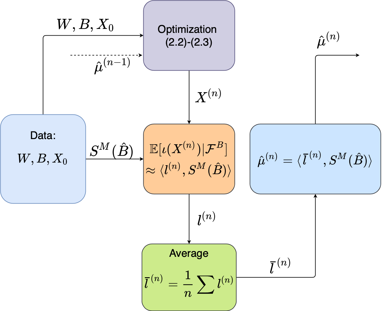
Figure 1: Flowchart of one iteration in the Sig-DFP Algorithm. Input: idiosyncratic noise Wπ‘ŠW, common noise B𝐡B, initial position X0subscript𝑋0X_{0} and measure flow ΞΌ^(nβˆ’1)superscript^πœ‡π‘›1\hat{\mu}^{(n-1)} from the last iteration. Output: measure flow ΞΌ^(n)superscript^πœ‡π‘›\hat{\mu}^{(n)} for the next iteration.

Having explained the key idea on how to approximate ΞΌπœ‡\mu efficiently, we describe the Sig-DFP algorithm in this subsection. The algorithm consists of repeatedly solving (2.2)–(2.3) for a given measure flow ΞΌπœ‡\mu using deep learning in the spirit of Han & E (2016), and passing the yielded ΞΌπœ‡\mu to the next iteration by using signatures. The flowchart of the idea is illustrated in Figure 1. Consider a partition Ο€πœ‹\pi of [0,T]:0=t0<β‹―<tL=T:0𝑇0subscript𝑑0β‹―subscript𝑑𝐿𝑇[0,T]:0=t_{0}<\cdots<t_{L}=T, denote by ΞΌ^(nβˆ’1)superscript^πœ‡π‘›1\hat{\mu}^{(n-1)} the given flow of measures at stage n𝑛n, the stochastic optimal control problem (2.2)–(2.3) is solved by

inf{Ξ±k}k=0Nβˆ’11Nβˆ‘i=1N(βˆ‘k=0Lβˆ’1f(tk,Xki,ΞΌ^k(nβˆ’1)(Ο‰i),Ξ±ki)Ξ”k\displaystyle\inf_{\{\alpha_{k}\}_{k=0}^{N-1}}\frac{1}{N}\sum_{i=1}^{N}\biggl{(}\sum_{k=0}^{L-1}f(t_{k},X_{k}^{i},\hat{\mu}^{(n-1)}_{k}(\omega^{i}),\alpha^{i}_{k})\Delta_{k}
+g(XLi,ΞΌ^L(nβˆ’1)(Ο‰i))),\displaystyle\hskip 60.00009pt+g(X^{i}_{L},\hat{\mu}_{L}^{(n-1)}(\omega^{i}))\biggr{)}, (4.4)
where ​Xk+1i=Xki+b​(tk,Xki,ΞΌ^k(nβˆ’1)​(Ο‰i),Ξ±ki)​ΔkwhereΒ subscriptsuperscriptπ‘‹π‘–π‘˜1subscriptsuperscriptπ‘‹π‘–π‘˜π‘subscriptπ‘‘π‘˜subscriptsuperscriptπ‘‹π‘–π‘˜subscriptsuperscript^πœ‡π‘›1π‘˜superscriptπœ”π‘–subscriptsuperscriptπ›Όπ‘–π‘˜subscriptΞ”π‘˜\displaystyle\text{where }X^{i}_{k+1}=X^{i}_{k}+b(t_{k},X^{i}_{k},\hat{\mu}^{(n-1)}_{k}(\omega^{i}),\alpha^{i}_{k})\Delta_{k}
+σ​(tk,Xki,ΞΌ^k(nβˆ’1)​(Ο‰i),Ξ±ki)​Δ​Wki𝜎subscriptπ‘‘π‘˜subscriptsuperscriptπ‘‹π‘–π‘˜subscriptsuperscript^πœ‡π‘›1π‘˜superscriptπœ”π‘–subscriptsuperscriptπ›Όπ‘–π‘˜Ξ”subscriptsuperscriptπ‘Šπ‘–π‘˜\displaystyle\hskip 60.00009pt+\sigma(t_{k},X^{i}_{k},\hat{\mu}^{(n-1)}_{k}(\omega^{i}),\alpha^{i}_{k})\Delta W^{i}_{k}
+Οƒ0​(tk,Xki,ΞΌ^k(nβˆ’1)​(Ο‰i),Ξ±ti)​Δ​Bki,superscript𝜎0subscriptπ‘‘π‘˜subscriptsuperscriptπ‘‹π‘–π‘˜subscriptsuperscript^πœ‡π‘›1π‘˜superscriptπœ”π‘–subscriptsuperscript𝛼𝑖𝑑Δsubscriptsuperscriptπ΅π‘–π‘˜\displaystyle\hskip 60.00009pt+\sigma^{0}(t_{k},X^{i}_{k},\hat{\mu}^{(n-1)}_{k}(\omega^{i}),\alpha^{i}_{t})\Delta B^{i}_{k}, (4.5)

where we replace the subscript tksubscriptπ‘‘π‘˜t_{k} by kπ‘˜k to simplify notations, and let Ξ”k=tk+1βˆ’tksubscriptΞ”π‘˜subscriptπ‘‘π‘˜1subscriptπ‘‘π‘˜\Delta_{k}=t_{k+1}-t_{k}, Δ​Wki=Wtk+1iβˆ’WtkiΞ”subscriptsuperscriptπ‘Šπ‘–π‘˜subscriptsuperscriptπ‘Šπ‘–subscriptπ‘‘π‘˜1subscriptsuperscriptπ‘Šπ‘–subscriptπ‘‘π‘˜\Delta W^{i}_{k}=W^{i}_{t_{k+1}}-W^{i}_{t_{k}}, Δ​Bki=Btk+1iβˆ’BtkiΞ”subscriptsuperscriptπ΅π‘–π‘˜subscriptsuperscript𝐡𝑖subscriptπ‘‘π‘˜1subscriptsuperscript𝐡𝑖subscriptπ‘‘π‘˜\Delta B^{i}_{k}=B^{i}_{t_{k+1}}-B^{i}_{t_{k}}. Here, we use the superscript i𝑖i to represent the it​hsuperscriptπ‘–π‘‘β„Ži^{th} sample path and ΞΌ^k(nβˆ’1)​(Ο‰i)subscriptsuperscript^πœ‡π‘›1π‘˜superscriptπœ”π‘–\hat{\mu}^{(n-1)}_{k}(\omega^{i}) to emphasize the stochastic measure’s dependence on the it​hsuperscriptπ‘–π‘‘β„Ži^{th} sample path of B𝐡B up to time tksubscriptπ‘‘π‘˜t_{k}. The control Ξ±ksubscriptπ›Όπ‘˜\alpha_{k} is then parameterized by neural networks (NNs) in the feedback form:

Ξ±ki:=αφ​(tk,Xki,ΞΌ^k(nβˆ’1)​(Ο‰i);Ο†),assignsuperscriptsubscriptπ›Όπ‘˜π‘–subscriptπ›Όπœ‘subscriptπ‘‘π‘˜subscriptsuperscriptπ‘‹π‘–π‘˜subscriptsuperscript^πœ‡π‘›1π‘˜superscriptπœ”π‘–πœ‘\alpha_{k}^{i}:=\alpha_{\varphi}(t_{k},X^{i}_{k},\hat{\mu}^{(n-1)}_{k}(\omega^{i});\varphi), (4.6)

where Ξ±Ο†subscriptπ›Όπœ‘\alpha_{\varphi} denotes the NN map with parameters Ο†πœ‘\varphi, and searching the infimum in (4.4) is translated into minimizing Ο†πœ‘\varphi. The yielded optimizer Ο†βˆ—superscriptπœ‘βˆ—\varphi^{\ast} gives Ξ±ki,βˆ—superscriptsubscriptπ›Όπ‘˜π‘–βˆ—\alpha_{k}^{i,\ast}, with which the optimized state process paths {Xi,βˆ—}i=1Nsuperscriptsubscriptsuperscriptπ‘‹π‘–βˆ—π‘–1𝑁\{X^{i,\ast}\}_{i=1}^{N} are simulated and its conditional law ℒ​(Xβˆ—|β„±B)β„’conditionalsuperscriptπ‘‹βˆ—superscriptℱ𝐡\mathcal{L}(X^{\ast}|\mathcal{F}^{B}), denoted by ΞΌ(n)superscriptπœ‡π‘›\mu^{(n)}, is approximated using signatures as described in SectionΒ 4.1. This finishes one iteration of fictitious play. Denote by ΞΌ~(n)superscript~πœ‡π‘›\tilde{\mu}^{(n)} the approximation of ΞΌ(n)superscriptπœ‡π‘›\mu^{(n)}, we then pass ΞΌ~(n)superscript~πœ‡π‘›\tilde{\mu}^{(n)} to the next iteration via updating ΞΌ^(n)=1n​μ~(n)+nβˆ’1n​μ^(nβˆ’1)superscript^πœ‡π‘›1𝑛superscript~πœ‡π‘›π‘›1𝑛superscript^πœ‡π‘›1\hat{\mu}^{(n)}=\frac{1}{n}\tilde{\mu}^{(n)}+\frac{n-1}{n}\hat{\mu}^{(n-1)} by averaging the coefficients in (4.3).

We summarize it in Algorithm 1, with implementation details deferred to AppendixΒ B. Note that the simulation of Xi,(n)superscript𝑋𝑖𝑛X^{i,(n)} and JB​(Ο†,ΞΌΒ―(nβˆ’1))subscriptπ½π΅πœ‘superscriptΒ―πœ‡π‘›1J_{B}(\varphi,\bar{\mu}^{(n-1)}) uses the equations (B.2) and (B.1) in AppendixΒ B, respectively.

Algorithm 1 The Sig-DFP Algorithm
Β Β Input: b,Οƒ,Οƒ0,f,g,ΞΉπ‘πœŽsubscript𝜎0π‘“π‘”πœ„b,\sigma,\sigma_{0},f,g,\iota and X0i,(Wtki)k=0L,(Btki)k=0Lsubscriptsuperscript𝑋𝑖0superscriptsubscriptsubscriptsuperscriptπ‘Šπ‘–subscriptπ‘‘π‘˜π‘˜0𝐿superscriptsubscriptsubscriptsuperscript𝐡𝑖subscriptπ‘‘π‘˜π‘˜0𝐿X^{i}_{0},(W^{i}_{t_{k}})_{k=0}^{L},(B^{i}_{t_{k}})_{k=0}^{L} for i=1,2,…,N𝑖12…𝑁i=1,2,\dots,N; Nroundsubscript𝑁roundN_{\text{round}}: rounds for FP; B𝐡B: minibatch size; Nbatchsubscript𝑁batchN_{\text{batch}}: number of minibatches.
Β Β Compute the signatures of B^0:tkisubscriptsuperscript^𝐡𝑖:0subscriptπ‘‘π‘˜\hat{B}^{i}_{0:t_{k}} for i=1,…,N𝑖1…𝑁i=1,\dots,N, k=1,…,Lπ‘˜1…𝐿k=1,\dots,L;
Β Β Initialize ΞΌ^(0)superscript^πœ‡0\hat{\mu}^{(0)}, Ο†πœ‘\varphi;
Β Β forΒ n=1𝑛1n=1 to Nroundsubscript𝑁roundN_{\text{round}}Β do
Β Β Β Β Β forΒ r=1π‘Ÿ1r=1 to Nbatchsubscript𝑁batchN_{\text{batch}}Β do
Β Β Β Β Β Β Β Β Simulate the rt​hsuperscriptπ‘Ÿπ‘‘β„Žr^{th} minibatch of Xi,(n)superscript𝑋𝑖𝑛X^{i,(n)} using ΞΌ^(nβˆ’1)superscript^πœ‡π‘›1\hat{\mu}^{(n-1)} and compute JB​(Ο†,ΞΌ^(nβˆ’1))subscriptπ½π΅πœ‘superscript^πœ‡π‘›1J_{B}(\varphi,\hat{\mu}^{(n-1)});
Β Β Β Β Β Β Β Β Minimize JB​(Ο†,ΞΌ^(nβˆ’1))subscriptπ½π΅πœ‘superscript^πœ‡π‘›1J_{B}(\varphi,\hat{\mu}^{(n-1)}) over Ο†πœ‘\varphi, then update Ξ±Ο†subscriptπ›Όπœ‘\alpha_{\varphi};
Β Β Β Β Β endΒ for
Β Β Β Β Β Simulate Xi,(n)superscript𝑋𝑖𝑛X^{i,(n)} with the optimized Ξ±Ο†βˆ—superscriptsubscriptπ›Όπœ‘βˆ—\alpha_{\varphi}^{\ast}, for i=1,…,N𝑖1…𝑁i=1,\dots,N;
Β Β Β Β Β Regress ι​(X0i,(n)),ι​(XL/2i,(n)),ι​(XLi,(n))πœ„subscriptsuperscript𝑋𝑖𝑛0πœ„subscriptsuperscript𝑋𝑖𝑛𝐿2πœ„subscriptsuperscript𝑋𝑖𝑛𝐿\iota(X^{i,(n)}_{0}),\iota(X^{i,(n)}_{L/2}),\iota(X^{i,(n)}_{L}) on SM​(B^0:0i)superscript𝑆𝑀subscriptsuperscript^𝐡𝑖:00S^{M}(\hat{B}^{i}_{0:0}), SM​(B^0:tL/2i)superscript𝑆𝑀subscriptsuperscript^𝐡𝑖:0subscript𝑑𝐿2S^{M}(\hat{B}^{i}_{0:t_{L/2}}), SM​(B^0:tLi)superscript𝑆𝑀subscriptsuperscript^𝐡𝑖:0subscript𝑑𝐿S^{M}(\hat{B}^{i}_{0:t_{L}}) to get l(n)superscript𝑙𝑛l^{(n)};
Β Β Β Β Β Update lΒ―(n)=nβˆ’1n​lΒ―(nβˆ’1)+1n​l(n)superscript¯𝑙𝑛𝑛1𝑛superscript¯𝑙𝑛11𝑛superscript𝑙𝑛\bar{l}^{(n)}=\frac{n-1}{n}\bar{l}^{(n-1)}+\frac{1}{n}l^{(n)};
Β Β Β Β Β Compute ΞΌ^(n)superscript^πœ‡π‘›\hat{\mu}^{(n)} by ΞΌ^k(n)​(Ο‰i)=⟨lΒ―(n),SM​(B^0:tki)⟩subscriptsuperscript^πœ‡π‘›π‘˜superscriptπœ”π‘–superscript¯𝑙𝑛superscript𝑆𝑀subscriptsuperscript^𝐡𝑖:0subscriptπ‘‘π‘˜\hat{\mu}^{(n)}_{k}(\omega^{i})=\langle\bar{l}^{(n)},S^{M}(\hat{B}^{i}_{0:t_{k}})\rangle, for i=1,2,…,N,k=1,…,Lformulae-sequence𝑖12β€¦π‘π‘˜1…𝐿i=1,2,\dots,N,k=1,\dots,L;
Β Β endΒ for
Β Β Output: the optimized Ξ±Ο†βˆ—superscriptsubscriptπ›Όπœ‘βˆ—\alpha_{\varphi}^{\ast} and lΒ―(Nround)superscript¯𝑙subscript𝑁round\bar{l}^{(N_{\text{round}})}.
Theorem 4.1 (Convergence analysis).

Let (Ξ±βˆ—(\alpha^{\ast},ΞΌβˆ—)\mu^{\ast}) be the mean-field equilibrium in DefinitionΒ 2.1, Ξ±(n)superscript𝛼𝑛\alpha^{(n)} be the optimal control, and ΞΌ(n)superscriptπœ‡π‘›\mu^{(n)} be the measure flow of the optimized state process after the nt​hsuperscriptπ‘›π‘‘β„Žn^{th} iteration of fictitious play, and ΞΌ~(n)superscript~πœ‡π‘›\tilde{\mu}^{(n)} be the approximation by truncated signatures. Under AssumptionΒ C.1 and supt∈[0,T]𝔼​[𝒲22​(ΞΌ~t(n),ΞΌt(n))]≀ϡsubscriptsupremum𝑑0𝑇𝔼delimited-[]superscriptsubscript𝒲22subscriptsuperscript~πœ‡π‘›π‘‘subscriptsuperscriptπœ‡π‘›π‘‘italic-Ο΅\displaystyle\sup_{t\in[0,T]}\mathbb{E}[\mathcal{W}_{2}^{2}(\tilde{\mu}^{(n)}_{t},\mu^{(n)}_{t})]\leq\epsilon, we have

supt∈[0,T]𝔼subscriptsupremum𝑑0𝑇𝔼\displaystyle\sup_{t\in[0,T]}\mathbb{E} [𝒲22​(ΞΌ~t(n),ΞΌtβˆ—)]+∫0T𝔼​|Ξ±t(n)βˆ’Ξ±tβˆ—|2​dtdelimited-[]superscriptsubscript𝒲22subscriptsuperscript~πœ‡π‘›π‘‘subscriptsuperscriptπœ‡βˆ—π‘‘superscriptsubscript0𝑇𝔼superscriptsuperscriptsubscript𝛼𝑑𝑛superscriptsubscriptπ›Όπ‘‘βˆ—2differential-d𝑑\displaystyle[\mathcal{W}_{2}^{2}(\tilde{\mu}^{(n)}_{t},\mu^{\ast}_{t})]+\int_{0}^{T}\mathbb{E}|\alpha_{t}^{(n)}-\alpha_{t}^{\ast}|^{2}\,\mathrm{d}t
≀C​(qn​supt∈[0,T]𝔼​[𝒲22​(ΞΌt(0),ΞΌtβˆ—)]+Ο΅),absent𝐢superscriptπ‘žπ‘›subscriptsupremum𝑑0𝑇𝔼delimited-[]superscriptsubscript𝒲22subscriptsuperscriptπœ‡0𝑑subscriptsuperscriptπœ‡βˆ—π‘‘italic-Ο΅\displaystyle\leq C(q^{n}\sup_{t\in[0,T]}\mathbb{E}[\mathcal{W}_{2}^{2}(\mu^{(0)}_{t},\mu^{\ast}_{t})]+\epsilon),

for some constants C>0𝐢0C>0 and 0<q<10π‘ž10<q<1, where 𝒲2subscript𝒲2\mathcal{W}_{2} denotes the 2-Wasserstein metric.

Moreover, if we consider a partition of [0,T]:0=t0<β‹―<tL=T:0𝑇0subscript𝑑0β‹―subscript𝑑𝐿𝑇[0,T]:0=t_{0}<\cdots<t_{L}=T, and define π​(t)=tkπœ‹π‘‘subscriptπ‘‘π‘˜\pi(t)=t_{k} for t∈[tk,tk+1)𝑑subscriptπ‘‘π‘˜subscriptπ‘‘π‘˜1t\in[t_{k},t_{k+1}) with β€–Ο€β€–=max1≀k<L⁑|tkβˆ’tkβˆ’1|normπœ‹subscript1π‘˜πΏsubscriptπ‘‘π‘˜subscriptπ‘‘π‘˜1\|\pi\|=\max_{1\leq k<L}|t_{k}-t_{k-1}|, then

Theorem 4.2 (Convergence in discrete time).

Let ΞΌtk(n)superscriptsubscriptπœ‡subscriptπ‘‘π‘˜π‘›\mu_{t_{k}}^{(n)} be the conditional law of the discretized optimal process Xtk(n)superscriptsubscript𝑋subscriptπ‘‘π‘˜π‘›X_{t_{k}}^{(n)} after the nt​hsuperscriptπ‘›π‘‘β„Žn^{th} iteration of fictitious play (cf. (4.5)), and ΞΌ~tk(n)subscriptsuperscript~πœ‡π‘›subscriptπ‘‘π‘˜\tilde{\mu}^{(n)}_{t_{k}} be the approximation by truncated signatures. Under AssumptionΒ C.1 and sup0≀k≀L𝔼​[𝒲22​(ΞΌ~tk(n),ΞΌtk(n))]≀ϡsubscriptsupremum0π‘˜πΏπ”Όdelimited-[]superscriptsubscript𝒲22subscriptsuperscript~πœ‡π‘›subscriptπ‘‘π‘˜subscriptsuperscriptπœ‡π‘›subscriptπ‘‘π‘˜italic-Ο΅\displaystyle\sup_{0\leq k\leq L}\mathbb{E}[\mathcal{W}_{2}^{2}(\tilde{\mu}^{(n)}_{t_{k}},\mu^{(n)}_{t_{k}})]\leq\epsilon, one has

supt∈[0,T]𝔼subscriptsupremum𝑑0𝑇𝔼\displaystyle\sup_{t\in[0,T]}\mathbb{E} [𝒲22​(ΞΌ~π​(t)(n),ΞΌtβˆ—)]+∫0T𝔼​|απ​(t)(n)βˆ’Ξ±tβˆ—|2​dtdelimited-[]superscriptsubscript𝒲22subscriptsuperscript~πœ‡π‘›πœ‹π‘‘subscriptsuperscriptπœ‡βˆ—π‘‘superscriptsubscript0𝑇𝔼superscriptsuperscriptsubscriptπ›Όπœ‹π‘‘π‘›superscriptsubscriptπ›Όπ‘‘βˆ—2differential-d𝑑\displaystyle[\mathcal{W}_{2}^{2}(\tilde{\mu}^{(n)}_{\pi(t)},\mu^{\ast}_{t})]+\int_{0}^{T}\mathbb{E}|\alpha_{\pi(t)}^{(n)}-\alpha_{t}^{\ast}|^{2}\,\mathrm{d}t
≀C​(qn​sup0≀k≀L𝔼​[𝒲22​(ΞΌtk(0),ΞΌtkβˆ—)]+Ο΅+β€–Ο€β€–),absent𝐢superscriptπ‘žπ‘›subscriptsupremum0π‘˜πΏπ”Όdelimited-[]superscriptsubscript𝒲22subscriptsuperscriptπœ‡0subscriptπ‘‘π‘˜subscriptsuperscriptπœ‡βˆ—subscriptπ‘‘π‘˜italic-Ο΅normπœ‹\displaystyle\leq C(q^{n}\sup_{0\leq k\leq L}\mathbb{E}[\mathcal{W}_{2}^{2}(\mu^{(0)}_{t_{k}},\mu^{\ast}_{t_{k}})]+\epsilon+\|\pi\|),

for some constants C>0𝐢0C>0 and 0<q<10π‘ž10<q<1, where Ξ±tk(n)=Ξ±^​(tk,Xtk,Ytk,ΞΌ~tk(nβˆ’1))superscriptsubscript𝛼subscriptπ‘‘π‘˜π‘›^𝛼subscriptπ‘‘π‘˜subscript𝑋subscriptπ‘‘π‘˜subscriptπ‘Œsubscriptπ‘‘π‘˜superscriptsubscript~πœ‡subscriptπ‘‘π‘˜π‘›1\alpha_{t_{k}}^{(n)}=\hat{\alpha}(t_{k},X_{t_{k}},Y_{t_{k}},\tilde{\mu}_{t_{k}}^{(n-1)}), and (Xt,Yt)subscript𝑋𝑑subscriptπ‘Œπ‘‘(X_{t},Y_{t}) solves (C.3) with ΞΌπœ‡\mu replaced by ΞΌ~tk(nβˆ’1)superscriptsubscript~πœ‡subscriptπ‘‘π‘˜π‘›1\tilde{\mu}_{t_{k}}^{(n-1)}.

The proofs of TheoremsΒ 4.1 and 4.2 are given in AppendixΒ C due to the page limit.

Remark that the Sig-DFP framework is flexible. We choose to solve (2.2)-(2.3) by direct parameterizing control policies Ξ±tsubscript𝛼𝑑\alpha_{t} for the sake of easy implementation and the possible exploration of multiple mean-field equilibria. If the equilibrium is unique, with proper conditions on the coefficients b,Οƒ,Οƒ0,fπ‘πœŽsuperscript𝜎0𝑓b,\sigma,\sigma^{0},f and g𝑔g, one can reformulate (2.2)-(2.3) into McKean-Vlasov FBSDEs or stochastic FP/HJB equations, and solve them by fictitious play and propagating the common noise using signatures.

5 Experiments

In this section, we present the performance of Sig-DFP for three examples: homogeneous, heterogeneous, and heterogeneous extended MFGs. A relative L2superscript𝐿2L^{2} metric will be used for performance measurement, defined for progressively measurable random processes as

LR2​(x,x^):=𝔼​[∫0Tβ€–xtβˆ’x^tβ€–2​dt]𝔼​[∫0Tβ€–xtβ€–2​dt],assignsubscriptsuperscript𝐿2𝑅π‘₯^π‘₯𝔼delimited-[]superscriptsubscript0𝑇superscriptnormsubscriptπ‘₯𝑑subscript^π‘₯𝑑2differential-d𝑑𝔼delimited-[]superscriptsubscript0𝑇superscriptnormsubscriptπ‘₯𝑑2differential-d𝑑L^{2}_{R}(x,\hat{x}):=\sqrt{\frac{\mathbb{E}[\int_{0}^{T}\|x_{t}-\hat{x}_{t}\|^{2}\,\mathrm{d}t]}{\mathbb{E}[\int_{0}^{T}\|x_{t}\|^{2}\,\mathrm{d}t]}}, (5.1)

where xπ‘₯x is a benchmark process and x^^π‘₯\hat{x} is its prediction. We shall use stochastic gradient descent (SGD) optimizer for all three experiments. Training processes are done on a server with Intel Core i9-9820X (10 cores, 3.30 GHz) and RTX 2080 Ti GPU, and training time will be reported in Appendix B. Implementation codes are available at https://github.com/mmin0/SigDFP.

Data Preparation. For all three experiments, the size of both training and test data is N=215𝑁superscript215N=2^{15}, and the size of validation data is N/2𝑁2N/2. We fix T=1𝑇1T=1 and discretize [0,1]01[0,1] by tk=k100,k=0,1,…,100formulae-sequencesubscriptπ‘‘π‘˜π‘˜100π‘˜01…100t_{k}=\frac{k}{100},\;k=0,1,\dots,100. Initial states are generated independently by X0i∼μ0similar-tosuperscriptsubscript𝑋0𝑖subscriptπœ‡0X_{0}^{i}\sim\mu_{0}, with ΞΌ0=U​(0,1)subscriptπœ‡0π‘ˆ01\mu_{0}=U(0,1) as the uniform distribution. The idiosyncratic Brownian motions Wπ‘ŠW and common noises B𝐡B are generated by antithetic variates for variance reduction, i.e., we generate the first half samples (Wi,Bi)superscriptπ‘Šπ‘–superscript𝐡𝑖(W^{i},B^{i}) and get the other half (βˆ’Wi,βˆ’Bi)superscriptπ‘Šπ‘–superscript𝐡𝑖(-W^{i},-B^{i}) by flipping.

Benchmarks. The examples below are carefully chosen with analytical benchmark solutions. Due to the space limit, we provide the details in AppendixΒ D.

Linear-Quadratic MFGs. We first consider a Linear-Quadratic MFG with common noise proposed in Carmona etΒ al. (2015), formulated as below:

infα𝔼{∫0T[Ξ±t22βˆ’qΞ±t(mtβˆ’Xt)+Ο΅2(mtβˆ’Xt)2]dt\displaystyle\inf_{\alpha}\mathbb{E}\biggl{\{}\int_{0}^{T}\left[\frac{\alpha_{t}^{2}}{2}-q\alpha_{t}(m_{t}-X_{t})+\frac{\epsilon}{2}(m_{t}-X_{t})^{2}\right]\,\mathrm{d}t
+c2(mTβˆ’XT)2},\displaystyle\hskip 50.00008pt+\frac{c}{2}(m_{T}-X_{T})^{2}\biggr{\}}, (5.2)
where ​d​Xt=[a​(mtβˆ’Xt)+Ξ±t]​d​twhereΒ dsubscript𝑋𝑑delimited-[]π‘Žsubscriptπ‘šπ‘‘subscript𝑋𝑑subscript𝛼𝑑d𝑑\displaystyle\text{where }\,\mathrm{d}X_{t}=[a(m_{t}-X_{t})+\alpha_{t}]\,\mathrm{d}t
+σ​(ρ​d​Bt+1βˆ’Ο2​d​Wt).𝜎𝜌dsubscript𝐡𝑑1superscript𝜌2dsubscriptπ‘Šπ‘‘\displaystyle\hskip 70.0001pt+\sigma(\rho\,\mathrm{d}B_{t}+\sqrt{1-\rho^{2}}\,\mathrm{d}W_{t}). (5.3)

Here mt=𝔼​[Xt|β„±tB]subscriptπ‘šπ‘‘π”Όdelimited-[]conditionalsubscript𝑋𝑑subscriptsuperscriptℱ𝐡𝑑m_{t}=\mathbb{E}[X_{t}|\mathcal{F}^{B}_{t}] is the conditional population mean, ρ∈[0,1]𝜌01\rho\in[0,1] characterizes the noise correlation between agents, and q,Ο΅,c,a,Οƒπ‘žitalic-Ο΅π‘π‘ŽπœŽq,\epsilon,c,a,\sigma are positive constants. The agents have homogeneous preferences and aim to minimize their individual costs. We assume q≀ϡ2π‘žsuperscriptitalic-Ο΅2q\leq\epsilon^{2} so that the Hamiltonian is jointly convex in state and control variables, ensuring a unique mean-field equilibrium.

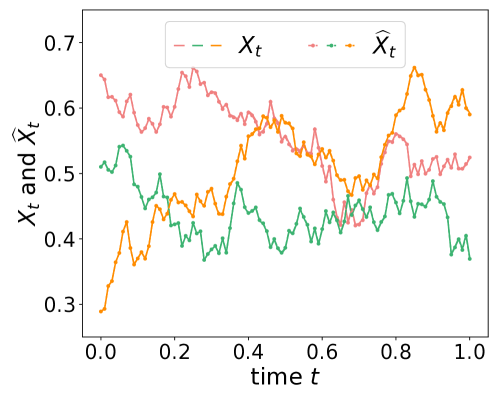
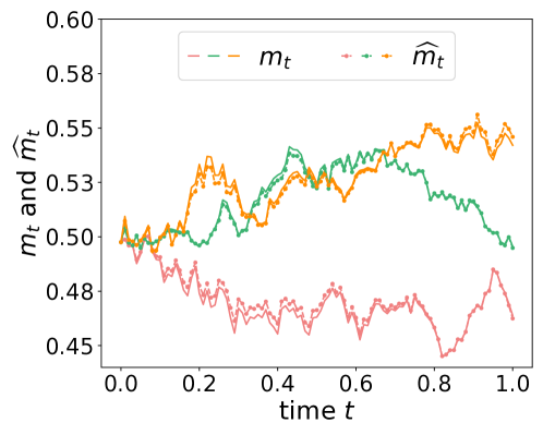
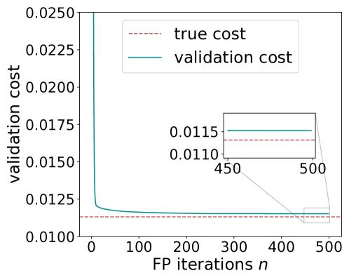
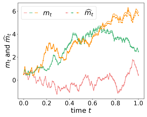
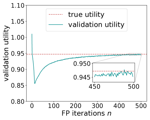
Training & Results. Ξ±Ο†subscriptπ›Όπœ‘\alpha_{\varphi} is a feedforward NN with two hidden layers of width 64. The truncated signature depth is chosen at M=2𝑀2M=2. The model is trained for 500500500 iterations of fictitious play. The optimized state process X^^𝑋\hat{X} and its conditional mean m^^π‘š\hat{m} generated by test data are shown in FiguresΒ 2a and 2b. The minimized cost after each iteration computed using validation data is given in FigureΒ 2c, where one can see a rapid convergence to the benchmark cost. During the experiments, we notice a slow convergence speed when using the average of m(n)superscriptπ‘šπ‘›m^{(n)} in (5.3). This is because the initial guess m(0)superscriptπ‘š0m^{(0)} is in general far from the truth. Therefore, for the first half of iterations, we simply use the previous-step result m(nβˆ’1)superscriptπ‘šπ‘›1m^{(n-1)}. The learning rate is set as 0.1 for the first half and 0.01 for the second half of training. The relative L2superscript𝐿2L^{2} errors for test data are listed in Table 1.

Table 1: Relative L2superscript𝐿2L^{2} errors on test data for the LQ MFG.
SDE Xtsubscript𝑋𝑑X_{t} Control Ξ±tsubscript𝛼𝑑\alpha_{t} Equilibrium mtsubscriptπ‘šπ‘‘m_{t}
LR2subscriptsuperscript𝐿2𝑅L^{2}_{R} 0.00310.00310.0031 0.00440.00440.0044 0.0580.0580.058
Refer to caption
(a) Xtsubscript𝑋𝑑X_{t}
Refer to caption
(b) mt=𝔼​(Xt|β„±tB)subscriptπ‘šπ‘‘π”Όconditionalsubscript𝑋𝑑superscriptsubscriptℱ𝑑𝐡m_{t}=\mathbb{E}(X_{t}|\mathcal{F}_{t}^{B})
Refer to caption
(c) Minimized Cost
Figure 2: Panels (a) and (b) give three trajectories of Xtsubscript𝑋𝑑X_{t}, mt=𝔼​[Xt|β„±bB]subscriptπ‘šπ‘‘π”Όdelimited-[]conditionalsubscript𝑋𝑑superscriptsubscriptℱ𝑏𝐡m_{t}=\mathbb{E}[X_{t}|\mathcal{F}_{b}^{B}] (solid lines) and their approximations (dashed lines) using different (X0,W,B)subscript𝑋0π‘Šπ΅(X_{0},W,B) from test data. Panel (c) shows the minimized cost computed using validation data over fictitious play iterations. Parameter choices are: Οƒ=0.2,q=1,a=1,Ο΅=1.5,ρ=0.2,c=1formulae-sequence𝜎0.2formulae-sequenceπ‘ž1formulae-sequenceπ‘Ž1formulae-sequenceitalic-Ο΅1.5formulae-sequence𝜌0.2𝑐1\sigma=0.2,q=1,a=1,\epsilon=1.5,\rho=0.2,c=1, x0∼U​(0,1)similar-tosubscriptπ‘₯0π‘ˆ01x_{0}\sim U(0,1).

Mean-Field Portfolio Game. Our second experiment is performed on a heterogeneous MFG proposed by Lacker & Zariphopoulou (2019), where the agent’s preference is different, characterized by a type vector ΢𝜁\zeta which is random and drawn at time 0. They all aim to maximize their exponential utility of terminal wealth compared to the population average:

supπ𝔼​[βˆ’exp⁑(βˆ’1δ​(XTβˆ’ΞΈβ€‹mT))],subscriptsupremumπœ‹π”Όdelimited-[]1𝛿subscriptπ‘‹π‘‡πœƒsubscriptπ‘šπ‘‡\sup_{\pi}\mathbb{E}\left[-\exp{\left(-\frac{1}{\delta}(X_{T}-\theta m_{T})\right)}\right], (5.4)

where the dynamics are

d​Xt=Ο€t​(μ​d​t+ν​d​Wt+σ​d​Bt),X0=ΞΎ.formulae-sequencedsubscript𝑋𝑑subscriptπœ‹π‘‘πœ‡dπ‘‘πœˆdsubscriptπ‘Šπ‘‘πœŽdsubscript𝐡𝑑subscript𝑋0πœ‰\,\mathrm{d}X_{t}=\pi_{t}(\mu\,\mathrm{d}t+\nu\,\mathrm{d}W_{t}+\sigma\,\mathrm{d}B_{t}),\quad X_{0}=\xi. (5.5)

Here mπ‘šm represents the conditional mean mt:=𝔼​[Xt|β„±tB]assignsubscriptπ‘šπ‘‘π”Όdelimited-[]conditionalsubscript𝑋𝑑subscriptsuperscriptℱ𝐡𝑑m_{t}:=\mathbb{E}[X_{t}|\mathcal{F}^{B}_{t}], and ΞΆ=(ΞΎ,Ξ΄,ΞΈ,ΞΌ,Ξ½,Οƒ)πœπœ‰π›Ώπœƒπœ‡πœˆπœŽ\zeta=(\xi,\delta,\theta,\mu,\nu,\sigma) is random.

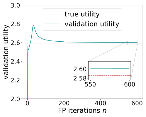
Training & Results. We use truncated signatures of depth M=2𝑀2M=2 and a feedforward NN πφsubscriptπœ‹πœ‘\pi_{\varphi} with 4 hidden layers333Since agents are heterogeneous characterized by their type vectors ΢𝜁\zeta, πφsubscriptπœ‹πœ‘\pi_{\varphi} takes (ΞΆ,t,Xt,mt)πœπ‘‘subscript𝑋𝑑subscriptπ‘šπ‘‘(\zeta,t,X_{t},m_{t}) as inputs. Hidden neurons in each layer are (64, 32, 32, 16). to approximate Ο€πœ‹\pi. We train our model with 500 iterations of fictitious play. The learning rate starts at 0.10.10.1 and is reduced by a factor of 555 every 200 rounds. The relative L2superscript𝐿2L^{2} errors evaluated under test data are listed in Table 2. Figure 3 compares X𝑋X and mπ‘šm to their approximations, and plots the maximized utilities.

Table 2: Relative L2superscript𝐿2L^{2} errors on test data for MF Portfolio Game.
SDE Xtsubscript𝑋𝑑X_{t} Invest Ο€tsubscriptπœ‹π‘‘\pi_{t} Equilibrium mtsubscriptπ‘šπ‘‘m_{t}
LR2subscriptsuperscript𝐿2𝑅L^{2}_{R} 0.0680.0680.068 0.0350.0350.035 0.0850.0850.085
Refer to caption
(a) Xtsubscript𝑋𝑑X_{t}
Refer to caption
(b) mt=𝔼​(Xt|β„±tB)subscriptπ‘šπ‘‘π”Όconditionalsubscript𝑋𝑑superscriptsubscriptℱ𝑑𝐡m_{t}=\mathbb{E}(X_{t}|\mathcal{F}_{t}^{B})
Refer to caption
(c) Maximized Utility
Figure 3: Panels (a) and (b) give three trajectories of Xtsubscript𝑋𝑑X_{t}, mt=𝔼​[Xt|β„±bB]subscriptπ‘šπ‘‘π”Όdelimited-[]conditionalsubscript𝑋𝑑superscriptsubscriptℱ𝑏𝐡m_{t}=\mathbb{E}[X_{t}|\mathcal{F}_{b}^{B}] (solid lines) and their approximations (dashed lines) using different (X0,W,B)subscript𝑋0π‘Šπ΅(X_{0},W,B) from test data. Panel (c) shows the maximized utility computed using validation data over fictitious play iterations. Parameter choices are: δ∼U​(5,5.5),μ∼U​(0.25,0.35),ν∼U​(0.2,0.4),θ∼U​(0,1),ΟƒβˆΌU​(0.2,0.4)formulae-sequencesimilar-toπ›Ώπ‘ˆ55.5formulae-sequencesimilar-toπœ‡π‘ˆ0.250.35formulae-sequencesimilar-toπœˆπ‘ˆ0.20.4formulae-sequencesimilar-toπœƒπ‘ˆ01similar-toπœŽπ‘ˆ0.20.4\delta\sim U(5,5.5),\mu\sim U(0.25,0.35),\nu\sim U(0.2,0.4),\theta\sim U(0,1),\sigma\sim U(0.2,0.4), ξ∼U​(0,1)similar-toπœ‰π‘ˆ01\xi\sim U(0,1).

Mean-Field Game of Optimal Consumption and Investment. Our last experiment considers an extended heterogeneous MFG proposed by Lacker & Soret (2020), where agents interact via both states and controls. The setup is similar to Lacker & Zariphopoulou (2019) except for including consumption and using power utilities. More precisely, each agent is characterized by a type vector ΞΆ=(ΞΎ,Ξ΄,ΞΈ,ΞΌ,Ξ½,Οƒ,Ο΅)πœπœ‰π›Ώπœƒπœ‡πœˆπœŽitalic-Ο΅\zeta=(\xi,\delta,\theta,\mu,\nu,\sigma,\epsilon), and the optimization problem reads

supΟ€,c𝔼​[∫0TU​(ct​Xt​(Ξ“t​mt)βˆ’ΞΈ;Ξ΄)​dt+ϡ​U​(XT​mTβˆ’ΞΈ;Ξ΄)],subscriptsupremumπœ‹π‘π”Όdelimited-[]superscriptsubscript0π‘‡π‘ˆsubscript𝑐𝑑subscript𝑋𝑑superscriptsubscriptΓ𝑑subscriptπ‘šπ‘‘πœƒπ›Ώdifferential-d𝑑italic-Ο΅π‘ˆsubscript𝑋𝑇subscriptsuperscriptπ‘šπœƒπ‘‡π›Ώ\sup_{\pi,c}\mathbb{E}\biggl{[}\int_{0}^{T}U(c_{t}X_{t}(\Gamma_{t}m_{t})^{-\theta};\delta)\,\mathrm{d}t+\epsilon U(X_{T}m^{-\theta}_{T};\delta)\biggr{]}, (5.6)

where U​(x;Ξ΄)=11βˆ’1δ​x1βˆ’1Ξ΄π‘ˆπ‘₯𝛿111𝛿superscriptπ‘₯11𝛿U(x;\delta)=\frac{1}{1-\frac{1}{\delta}}x^{1-\frac{1}{\delta}}, Ξ΄β‰ 1𝛿1\delta\neq 1, Xtsubscript𝑋𝑑X_{t} follows

d​Xt=Ο€t​Xt​(μ​d​t+ν​d​Wt+σ​d​Bt)βˆ’ct​Xt​d​t,dsubscript𝑋𝑑subscriptπœ‹π‘‘subscriptπ‘‹π‘‘πœ‡dπ‘‘πœˆdsubscriptπ‘Šπ‘‘πœŽdsubscript𝐡𝑑subscript𝑐𝑑subscript𝑋𝑑d𝑑\,\mathrm{d}X_{t}=\pi_{t}X_{t}(\mu\,\mathrm{d}t+\nu\,\mathrm{d}W_{t}+\sigma\,\mathrm{d}B_{t})-c_{t}X_{t}\,\mathrm{d}t, (5.7)

and X0=ΞΎsubscript𝑋0πœ‰X_{0}=\xi. Here Ξ“t=exp⁑𝔼​[log⁑ct|β„±tB]subscriptΓ𝑑𝔼delimited-[]conditionalsubscript𝑐𝑑subscriptsuperscriptℱ𝐡𝑑\Gamma_{t}=\exp\mathbb{E}[\log c_{t}|\mathcal{F}^{B}_{t}] and mt=exp⁑𝔼​[log⁑Xt|β„±tB]subscriptπ‘šπ‘‘π”Όdelimited-[]conditionalsubscript𝑋𝑑subscriptsuperscriptℱ𝐡𝑑m_{t}=\exp\mathbb{E}[\log X_{t}|\mathcal{F}^{B}_{t}] are the mean-field interactions from consumption and wealth.

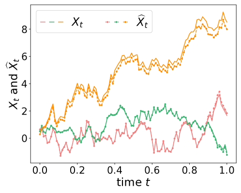
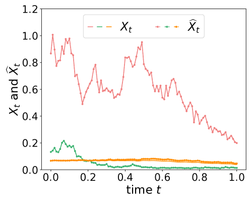
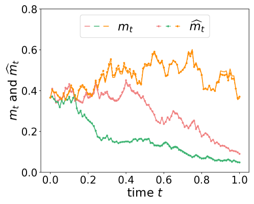
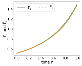
Training & Results. For this experiment, we use truncated signatures of depth M=4𝑀4M=4. The optimal controls (Ο€t,ct)0≀t≀1subscriptsubscriptπœ‹π‘‘subscript𝑐𝑑0𝑑1(\pi_{t},c_{t})_{0\leq t\leq 1} are parameterized by two neural networks πφsubscriptπœ‹πœ‘\pi_{\varphi} and cΟ†subscriptπ‘πœ‘c_{\varphi}, each with three hidden layers.444Due to the nature of heterogeneous extended MFG, both Ξ±Ο†subscriptπ›Όπœ‘\alpha_{\varphi} and cΟ†subscriptπ‘πœ‘c_{\varphi} take (ΞΆt,t,Xt,mt,Ξ“t)subscriptπœπ‘‘π‘‘subscript𝑋𝑑subscriptπ‘šπ‘‘subscriptΓ𝑑(\zeta_{t},t,X_{t},m_{t},\Gamma_{t}) as inputs. Hidden neurons in each layer are (64, 64, 64). Due to the extended mean-field interaction term Ξ“tsubscriptΓ𝑑\Gamma_{t}, we will propagate two conditional distribution flows, i.e., two linear functionals lΒ―(n),lΒ―c(n)superscript¯𝑙𝑛superscriptsubscript¯𝑙𝑐𝑛\bar{l}^{(n)},\bar{l}_{c}^{(n)} during each iteration of fictitious play. Instead of estimating mt,Ξ“tsubscriptπ‘šπ‘‘subscriptΓ𝑑m_{t},\Gamma_{t} directly, we estimate 𝔼​[log⁑Xt|β„±tB],𝔼​[log⁑ct|β„±tB]𝔼delimited-[]conditionalsubscript𝑋𝑑subscriptsuperscriptℱ𝐡𝑑𝔼delimited-[]conditionalsubscript𝑐𝑑subscriptsuperscriptℱ𝐡𝑑\mathbb{E}[\log X_{t}|\mathcal{F}^{B}_{t}],\mathbb{E}[\log c_{t}|\mathcal{F}^{B}_{t}] by ⟨lΒ―(n),S4​(B0:t)⟩superscript¯𝑙𝑛superscript𝑆4subscript𝐡:0𝑑\langle\bar{l}^{(n)},S^{4}(B_{0:t})\rangle, ⟨lΒ―c(n),S4​(B0:t)⟩superscriptsubscript¯𝑙𝑐𝑛superscript𝑆4subscript𝐡:0𝑑\langle\bar{l}_{c}^{(n)},S^{4}(B_{0:t})\rangle and then take exponential to get mt,Ξ“tsubscriptπ‘šπ‘‘subscriptΓ𝑑m_{t},\Gamma_{t}. To ensure the non-negativity condition of Xtsubscript𝑋𝑑X_{t}, we evolve log⁑Xtsubscript𝑋𝑑\log X_{t} according to (D.4) and then take exponential to get Xtsubscript𝑋𝑑X_{t}. For optimal consumption, cΟ†subscriptπ‘πœ‘c_{\varphi} is used to predicted log⁑ctsubscript𝑐𝑑\log c_{t} and thus exp⁑cΟ†subscriptπ‘πœ‘\exp c_{\varphi} gives the predicted ctsubscript𝑐𝑑c_{t}. With 600 iterations of fictitious play and a learning rate of 0.1 decaying by a factor of 5 for every 200 iterations, the relative L2superscript𝐿2L^{2} errors for test data are listed in Table 3. Figure 4 compares X𝑋X and mπ‘šm to their approximations, and plots the maximized utilities. Plots of Ο€tsubscriptπœ‹π‘‘\pi_{t}, ctsubscript𝑐𝑑c_{t}, Ξ“t=exp⁑𝔼​(log⁑ct|β„±tB)subscriptΓ𝑑𝔼conditionalsubscript𝑐𝑑subscriptsuperscriptℱ𝐡𝑑\Gamma_{t}=\exp\mathbb{E}(\log c_{t}|\mathcal{F}^{B}_{t}) are provided in AppendixΒ E.

Table 3: Relative L2superscript𝐿2L^{2} errors on test data for Optimal Consumption and Investment MFG.
Invest Ο€tsubscriptπœ‹π‘‘\pi_{t} Consumption ctsubscript𝑐𝑑c_{t} mtsubscriptπ‘šπ‘‘m_{t} Ξ“tsubscriptΓ𝑑\Gamma_{t}
LR2subscriptsuperscript𝐿2𝑅L^{2}_{R} 0.11260.11260.1126 0.06140.06140.0614 0.02790.02790.0279 0.01210.01210.0121
Refer to caption
(a) Xtsubscript𝑋𝑑X_{t}
Refer to caption
(b) mt=exp⁑𝔼​(log⁑Xt|β„±tB)subscriptπ‘šπ‘‘π”Όconditionalsubscript𝑋𝑑subscriptsuperscriptℱ𝐡𝑑m_{t}=\exp\mathbb{E}(\log X_{t}|\mathcal{F}^{B}_{t})
Refer to caption
(c) Maximized Utility
Figure 4: Panels (a) and (b) give three trajectories of Xtsubscript𝑋𝑑X_{t} and mt=exp⁑𝔼​(log⁑Xt|β„±tB)subscriptπ‘šπ‘‘π”Όconditionalsubscript𝑋𝑑subscriptsuperscriptℱ𝐡𝑑m_{t}=\exp\mathbb{E}(\log X_{t}|\mathcal{F}^{B}_{t}) (solid lines) and their approximation (dashed lines) using different (X0,W,B)subscript𝑋0π‘Šπ΅(X_{0},W,B) from test data. Panel (c) shows the maximized utility computed using validation data over fictitious play iterations. Parameter choices are: δ∼U​(2,2.5),μ∼U​(0.25,0.35),ν∼U​(0.2,0.4),ΞΈ,ξ∼U​(0,1),ΟƒβˆΌU​(0.2,0.4)formulae-sequencesimilar-toπ›Ώπ‘ˆ22.5formulae-sequencesimilar-toπœ‡π‘ˆ0.250.35formulae-sequencesimilar-toπœˆπ‘ˆ0.20.4πœƒformulae-sequencesimilar-toπœ‰π‘ˆ01similar-toπœŽπ‘ˆ0.20.4\delta\sim U(2,2.5),\mu\sim U(0.25,0.35),\nu\sim U(0.2,0.4),\theta,\xi\sim U(0,1),\sigma\sim U(0.2,0.4), ϡ∼U​(0.5,1)similar-toitalic-Ο΅π‘ˆ0.51\epsilon\sim U(0.5,1).

Comparison with the nested algorithm. We run both Sig-DFP and the nested algorithm for the training data size of (INP, CNP)=(24,24),(26,26)​(28,28)absentsuperscript24superscript24superscript26superscript26superscript28superscript28=(2^{4},2^{4}),\;(2^{6},2^{6})\;(2^{8},2^{8}), where INP means the number of individual noise paths and CNP means the number of common noise paths. From the comparisons of running time, memory, and relative L2superscript𝐿2L^{2} errors in TablesΒ 4 and 5, one can see that the accuracy is mainly affected by the size of (INP, CNP) used for training the neural network. Sig-DFP has the advantage of reducing memory request and running time, which allows it to use a larger size of data, e.g., (INP, CNP)=(215,215)absentsuperscript215superscript215=(2^{15},2^{15}), to produce much better accuracy. The quadratic growth of memory in the nested algorithm, evidenced by the first three columns of data in TablesΒ 4 (least squares growth rate β‰ˆ2absent2\approx 2), makes us unable to run the nested algorithm beyond (28,28)superscript28superscript28(2^{8},2^{8}) in our current computing environment due to its high demand for memory.

Table 4: Running time (hours) and Memory (GBs) comparisons between Sig-DFP and the nested algorithm for different (INP, CNP)’s. INP == # of individual noise paths, CNP == # of common noise paths, and NA == Not Available due to high demand for memory.
(INP, CNP) (24,24)superscript24superscript24(2^{4},2^{4}) (26,26)superscript26superscript26(2^{6},2^{6}) (28,28)superscript28superscript28(2^{8},2^{8}) (212,212)superscript212superscript212(2^{12},2^{12}) (215,215)superscript215superscript215(2^{15},2^{15})
Nested Algorithm (0.09,2.1)0.092.1(0.09,2.1) (0.46,4.1)0.464.1(0.46,4.1) (4.3,43.5)4.343.5(4.3,43.5) NA NA
Sig-DFP (0.09,1.9)0.091.9(0.09,1.9) (0.1,2.0)0.12.0(0.1,2.0) (0.17,2.3)0.172.3(0.17,2.3) (0.33,4.8)0.334.8(0.33,4.8) (1.3,27)1.327(1.3,27)
Table 5: The comparisons of relative L2superscript𝐿2L^{2} errors on (Ο€,c)πœ‹π‘(\pi,c) between Sig-DFP and the nested algorithm for different (INP, CNP)’s. INP == # of individual noise paths, CNP == # of common noise paths, and NA == Not Available due to high demand for memory.
(INP, CNP) (24,24)superscript24superscript24(2^{4},2^{4}) (26,26)superscript26superscript26(2^{6},2^{6}) (28,28)superscript28superscript28(2^{8},2^{8}) (212,212)superscript212superscript212(2^{12},2^{12}) (215,215)superscript215superscript215(2^{15},2^{15})
Nested Algorithm (53%,44%)percent53percent44(53\%,44\%) (36%,41%)percent36percent41(36\%,41\%) (79.4%,16.2%)percent79.4percent16.2(79.4\%,16.2\%) NA NA
Sig-DFP (85.8%,48.1%)percent85.8percent48.1(85.8\%,48.1\%) (43.3%,44.9%)percent43.3percent44.9(43.3\%,44.9\%) (49%,43%)percent49percent43(49\%,43\%) (18%,38%)percent18percent38(18\%,38\%) (11%,6%)percent11percent6(11\%,6\%)
Table 6: The comparisons of running time (hours) for different signature depth M𝑀M and dimension n0subscript𝑛0n_{0} using (INP, CNP)=(215,215)absentsuperscript215superscript215\small=(2^{15},2^{15}) .
(n0subscript𝑛0n_{0}, Depth M𝑀M) (1,1)11(1,1) (1,2)12(1,2) (1,3)13(1,3) (1,4)14(1,4) (5,1)51(5,1) (5,2)52(5,2) (5,3)53(5,3) (5,4)54(5,4)
Running Time (hours) 1.21.21.2 1.21.21.2 1.21.21.2 1.31.31.3 1.21.21.2 1.31.31.3 1.51.51.5 2.62.62.6

Comparisons of running time for different signature depth M𝑀M and dimension n0subscript𝑛0n_{0}. We choose the data size (INP, CNP)=(215,215)absentsuperscript215superscript215=(2^{15},2^{15}) and compare the running time for different (n0,M)subscript𝑛0𝑀(n_{0},M)’s in TableΒ 6. Choosing M=1,2,3,4𝑀1234M=1,2,3,4 yield the relative L2superscript𝐿2L^{2} errors of controls (Ο€,c)πœ‹π‘(\pi,c) as (15.9%,9.5%)percent15.9percent9.5(15.9\%,9.5\%), (11.4%,6.3%)percent11.4percent6.3(11.4\%,6.3\%), (11.4%,6.3%)percent11.4percent6.3(11.4\%,6.3\%) and (11.3%,6.1%)percent11.3percent6.1(11.3\%,6.1\%) for n0=1subscript𝑛01n_{0}=1, respectively. Note that, compared to M=1𝑀1M=1, taking M=2𝑀2M=2 improves the accuracy significantly but not M=3,4𝑀34M=3,4. This is because the curves of log⁑(ct)subscript𝑐𝑑\log(c_{t}) and log⁑(Xtβˆ—)superscriptsubscript𝑋𝑑\log(X_{t}^{*}) are approximately either linear or quadratic in t𝑑t, as shown in FigureΒ 5 in AppendixΒ E after taking a logarithm, which implies that the signatures of depth M=2𝑀2M=2 will be sufficient to produce good accuracy. We remark that Sig-DFP has no difficulty computing high-dimensional problems, evidenced by the running time of n0=5subscript𝑛05n_{0}=5 cases in TableΒ 6. We focus on one-dimensional problems since, to our best knowledge, the closed-form non-trivial solutions only exist in one-dimensional cases, which can serve as the benchmark solutions. More details about n0=5subscript𝑛05n_{0}=5 are given in AppendixΒ F.

6 Conclusion

In this paper, we propose a novel single-loop algorithm, named signatured deep fictitious play, for solving mean-field games (MFGs) with common noise. We incorporate signature from rough path theory into the strategy of deep fictitious play (Hu, 2021; Han & Hu, 2020; Han etΒ al., 2020), and avoid the nested-loop structure in existing machine learning methods, which reduces the computational cost significantly. Analysis of the complexity and convergence for the proposed algorithm is provided. The effectiveness of the algorithm is justified by three applications, and in particular, we report the first deep learning work to deal with extended MFGs with common noise. In the future, we shall study deep learning algorithms for MFGs with common noise in more general settings (Hu & Zariphopoulou, 2021).

Acknowledgement

R.H.Β was partially supported by NSF grant DMS-1953035, the Faculty Career Development Award and the Research Assistance Program Award, University of California, Santa Barbara. M.M. and R.H. are grateful to the reviewers for their valuable and constructive comments.

References

  • Achdou & Lasry (2019) Achdou, Y. and Lasry, J.-M. Mean field games for modeling crowd motion. In Contributions to partial differential equations and applications, pp.Β  17–42. Springer, 2019.
  • Achdou etΒ al. (2017) Achdou, Y., Bardi, M., and Cirant, M. Mean field games models of segregation. Mathematical Models and Methods in Applied Sciences, 27(01):75–113, 2017.
  • Ahuja (2015) Ahuja, S. Mean Field Games with Common Noise. PhD thesis, Stanford University, 2015.
  • Ahuja (2016) Ahuja, S. Wellposedness of mean field games with common noise under a weak monotonicity condition. SIAM Journal on Control and Optimization, 54(1):30–48, 2016.
  • Angiuli etΒ al. (2020) Angiuli, A., Fouque, J.-P., and LauriΓ¨re, M. Unified reinforcement Q-learning for mean field game and control problems. arXiv preprint arXiv:2006.13912, 2020.
  • Bensoussan etΒ al. (2015) Bensoussan, A., Frehse, J., and Yam, S. C.Β P. The master equation in mean field theory. Journal de MathΓ©matiques Pures et AppliquΓ©es, 103(6):1441–1474, 2015.
  • Boedihardjo etΒ al. (2016) Boedihardjo, H., Geng, X., Lyons, T., and Yang, D. The signature of a rough path: uniqueness. Advances in Mathematics, 293:720–737, 2016.
  • Bonnier etΒ al. (2019) Bonnier, P., Kidger, P., Arribas, I.Β P., Salvi, C., and Lyons, T. Deep signature transforms. In Advances in Neural Information Processing Systems 32 (NeurIPS), 2019.
  • Briani & Cardaliaguet (2018) Briani, A. and Cardaliaguet, P. Stable solutions in potential mean field game systems. Nonlinear Differential Equations and Applications NoDEA, 25(1):1–26, 2018.
  • Brown (1949) Brown, G.Β W. Some notes on computation of games solutions. Technical report, RAND CORP SANTA MONICA CA, 1949.
  • Brown (1951) Brown, G.Β W. Iterative solution of games by fictitious play. Activity analysis of production and allocation, 13(1):374–376, 1951.
  • Caines etΒ al. (2017) Caines, P.Β E., Huang, M., and MalhamΓ©, R.Β P. Mean field games. In Handbook of Dynamic Game Theory, pp.Β  1–28. Springer, 2017.
  • Cardaliaguet & Hadikhanloo (2017) Cardaliaguet, P. and Hadikhanloo, S. Learning in mean field games: the fictitious play. ESAIM: Control, Optimisation and Calculus of Variations, 23(2):569–591, 2017.
  • Cardaliaguet & Lehalle (2018) Cardaliaguet, P. and Lehalle, C.-A. Mean field game of controls and an application to trade crowding. Mathematics and Financial Economics, 12(3):335–363, 2018.
  • Cardaliaguet etΒ al. (2019) Cardaliaguet, P., Delarue, F., Lasry, J.-M., and Lions, P.-L. The Master Equation and the Convergence Problem in Mean Field Games:(AMS-201), volume 201. Princeton University Press, 2019.
  • Carmona & Delarue (2018a) Carmona, R. and Delarue, F. Probabilistic Theory of Mean Field Games with Applications I. Springer, 2018a.
  • Carmona & Delarue (2018b) Carmona, R. and Delarue, F. Probabilistic Theory of Mean Field Games with Applications II. Springer, 2018b.
  • Carmona & LauriΓ¨re (2019) Carmona, R. and LauriΓ¨re, M. Convergence analysis of machine learning algorithms for the numerical solution of mean field control and games: II–the finite horizon case. arXiv preprint arXiv:1908.01613, 2019.
  • Carmona & Zhu (2016) Carmona, R. and Zhu, X. A probabilistic approach to mean field games with major and minor players. Annals of Applied Probability, 26(3):1535–1580, 2016.
  • Carmona etΒ al. (2015) Carmona, R., Fouque, J.-P., and Sun, L.-H. Mean field games and systemic risk. Communications in Mathematical Sciences, 13(4):911–933, 2015.
  • Carmona etΒ al. (2016) Carmona, R., Delarue, F., and Lacker, D. Mean field games with common noise. Annals of Probability, 44(6):3740–3803, 2016.
  • Chevyrev & Oberhauser (2018) Chevyrev, I. and Oberhauser, H. Signature moments to characterize laws of stochastic processes. arXiv preprint arXiv:1810.10971, 2018.
  • Djehiche etΒ al. (2017) Djehiche, B., Tcheukam, A., and Tembine, H. A mean-field game of evacuation in multilevel building. IEEE Transactions on Automatic Control, 62(10):5154–5169, 2017.
  • Elie etΒ al. (2020a) Elie, R., Hubert, E., and Turinici, G. Contact rate epidemic control of COVID-19: an equilibrium view. Mathematical Modelling of Natural Phenomena, 15:35, 2020a.
  • Elie etΒ al. (2020b) Elie, R., PΓ©rolat, J., LauriΓ¨re, M., Geist, M., and Pietquin, O. On the convergence of model free learning in mean field games. In Proceedings of the AAAI Conference on Artificial Intelligence, volumeΒ 34, pp.Β  7143–7150, 2020b.
  • Friz & Victoir (2010) Friz, P.Β K. and Victoir, N.Β B. Multidimensional stochastic processes as rough paths: theory and applications, volume 120. Cambridge University Press, 2010.
  • Goodfellow etΒ al. (2014) Goodfellow, I.Β J., Pouget-Abadie, J., Mirza, M., Xu, B., Warde-Farley, D., Ozair, S., Courville, A., and Bengio, Y. Generative adversarial nets. In Advances in Neural Information Processing Systems 27 (NIPS), 2014.
  • Graber (2016) Graber, P.Β J. Linear quadratic mean field type control and mean field games with common noise, with application to production of an exhaustible resource. Applied Mathematics & Optimization, 74(3):459–486, 2016.
  • Guo etΒ al. (2019) Guo, X., Hu, A., Xu, R., and Zhang, J. Learning mean-field games. In Advances in Neural Information Processing Systems 32 (NeurIPS), 2019.
  • Han & E (2016) Han, J. and E, W. Deep learning approximation for stochastic control problems. Deep Reinforcement Learning Workshop, NIPS, 2016.
  • Han & Hu (2020) Han, J. and Hu, R. Deep fictitious play for finding Markovian Nash equilibrium in multi-agent games. In Mathematical and Scientific Machine Learning (MSML), volume 107, pp.Β  221–245. PMLR, 2020.
  • Han etΒ al. (2020) Han, J., Hu, R., and Long, J. Convergence of deep fictitious play for stochastic differential games. arXiv preprint arXiv:2008.05519, 2020.
  • Han etΒ al. (2021) Han, J., Hu, R., and Long, J. A class of dimensionality-free metrics for the convergence of empirical measures. arXiv preprint arXiv:2104.12036, 2021.
  • Hu (2021) Hu, R. Deep fictitious play for stochastic differential games. Communications in Mathematical Sciences, 19(2):325–353, 2021.
  • Hu & Zariphopoulou (2021) Hu, R. and Zariphopoulou, T. N-player and mean-field games in ItΓ΄-diffusion markets with competitive or homophilous interaction. arXiv preprint arXiv:2106.00581, 2021.
  • Huang (2010) Huang, M. Large-population LQG games involving a major player: the Nash certainty equivalence principle. SIAM Journal on Control and Optimization, 48(5):3318–3353, 2010.
  • Huang etΒ al. (2006) Huang, M., MalhamΓ©, R.Β P., and Caines, P.Β E. Large population stochastic dynamic games: closed-loop mckean-vlasov systems and the nash certainty equivalence principle. Communications in Information & Systems, 6(3):221–252, 2006.
  • Hubert & Turinici (2018) Hubert, E. and Turinici, G. Nash-MFG equilibrium in a SIR model with time dependent newborn vaccination. Ricerche di matematica, 67(1):227–246, 2018.
  • Kidger & Lyons (2020) Kidger, P. and Lyons, T. Signatory: differentiable computations of the signature and logsignature transforms, on both CPU and GPU. arXiv preprint arXiv:2001.00706, 2020.
  • KirΓ‘ly & Oberhauser (2019) KirΓ‘ly, F.Β J. and Oberhauser, H. Kernels for sequentially ordered data. Journal of Machine Learning Research, 20(31):1–45, 2019.
  • Lachapelle etΒ al. (2016) Lachapelle, A., Lasry, J.-M., Lehalle, C.-A., and Lions, P.-L. Efficiency of the price formation process in presence of high frequency participants: a mean field game analysis. Mathematics and Financial Economics, 10(3):223–262, 2016.
  • Lacker & Soret (2020) Lacker, D. and Soret, A. Many-player games of optimal consumption and investment under relative performance criteria. Mathematics and Financial Economics, 14(2):263–281, 2020.
  • Lacker & Webster (2015) Lacker, D. and Webster, K. Translation invariant mean field games with common noise. Electronic Communications in Probability, 20, 2015.
  • Lacker & Zariphopoulou (2019) Lacker, D. and Zariphopoulou, T. Mean field and n-agent games for optimal investment under relative performance criteria. Mathematical Finance, 29(4):1003–1038, 2019.
  • Lasry & Lions (2007) Lasry, J.-M. and Lions, P.-L. Mean field games. Japanese Journal of Mathematics, 2(1):229–260, 2007.
  • Lin etΒ al. (2020) Lin, A.Β T., Fung, S.Β W., Li, W., Nurbekyan, L., and Osher, S.Β J. APAC-Net: Alternating the population and agent control via two neural networks to solve high-dimensional stochastic mean field games. arXiv preprint arXiv:2002.10113, 2020.
  • Lyons & Qian (2002) Lyons, T. and Qian, Z. System control and rough paths. Oxford University Press, 2002.
  • Lyons etΒ al. (2007) Lyons, T.Β J., Caruana, M., and LΓ©vy, T. Differential equations driven by rough paths. Springer, 2007.
  • Min & Ichiba (2020) Min, M. and Ichiba, T. Convolutional signature for sequential data. arXiv preprint arXiv:2009.06719, 2020.
  • Ni etΒ al. (2020) Ni, H., Szpruch, L., Wiese, M., Liao, S., and Xiao, B. Conditional Sig-Wasserstein GANs for time series generation. arXiv preprint arXiv:2006.05421, 2020.
  • Nourian & Caines (2013) Nourian, M. and Caines, P.Β E. Ο΅italic-Ο΅\epsilon-Nash mean field game theory for nonlinear stochastic dynamical systems with major and minor agents. SIAM Journal on Control and Optimization, 51(4):3302–3331, 2013.
  • Pedregosa etΒ al. (2011) Pedregosa, F., Varoquaux, G., Gramfort, A., Michel, V., Thirion, B., Grisel, O., Blondel, M., Prettenhofer, P., Weiss, R., Dubourg, V., Vanderplas, J., Passos, A., Cournapeau, D., Brucher, M., Perrot, M., and Duchesnay, E. Scikit-learn: Machine learning in Python. Journal of Machine Learning Research, 12:2825–2830, 2011.
  • Perrin etΒ al. (2020) Perrin, S., PΓ©rolat, J., LauriΓ¨re, M., Geist, M., Elie, R., and Pietquin, O. Fictitious play for mean field games: Continuous time analysis and applications. In Advances in Neural Information Processing Systems 33 (NeurIPS), 2020.
  • Ruthotto etΒ al. (2020) Ruthotto, L., Osher, S.Β J., Li, W., Nurbekyan, L., and Fung, S.Β W. A machine learning framework for solving high-dimensional mean field game and mean field control problems. Proceedings of the National Academy of Sciences, 117(17):9183–9193, 2020.
  • Tiwari etΒ al. (2019) Tiwari, N., Ghosh, A., and Aggarwal, V. Reinforcement learning for mean field game. arXiv preprint arXiv:1905.13357, 2019.
  • Toth & Oberhauser (2020) Toth, C. and Oberhauser, H. Bayesian learning from sequential data using gaussian processes with signature covariances. In Proceedings of the 37th International Conference on Machine Learning (ICML), volume 119, pp.Β  9548–9560. PMLR, 2020.
  • Xuan etΒ al. (2021) Xuan, Y., Blkin, R., Han, J., Hu, R., and Ceniceros, H.Β D. Optimal policies for a pandemic: A stochastic game approach and a deep learning algorithm. In Mathematical and Scientific Machine Learning (MSML), 2021. Accepted.

Appendix A Preliminaries on Rough Path Theory and Signatures

In this appendix, we shall follow Lyons & Qian (2002); Lyons etΒ al. (2007); Friz & Victoir (2010) and briefly introduce rough path theory and signatures. We will also give the proof of LemmaΒ 4.1 using the factorial decay property of signatures. Denote by Ξ”TsubscriptΔ𝑇\Delta_{T} the simplex {(s,t)∈[0,T]2:0≀s≀t≀T}conditional-set𝑠𝑑superscript0𝑇20𝑠𝑑𝑇\{(s,t)\in[0,T]^{2}:0\leq s\leq t\leq T\}, and by Tn​(ℝd)=⨁k=0n(ℝd)⨂ksuperscript𝑇𝑛superscriptℝ𝑑superscriptsubscriptdirect-sumπ‘˜0𝑛superscriptsuperscriptℝ𝑑tensor-productπ‘˜T^{n}(\mathbb{R}^{d})=\bigoplus_{k=0}^{n}(\mathbb{R}^{d})^{\bigotimes k} the truncated tensor algebra.

Definition A.1 (Multiplicative Functional).

Let 𝕏:Ξ”Tβ†’Tn​(ℝd):𝕏→subscriptΔ𝑇superscript𝑇𝑛superscriptℝ𝑑\mathds{X}:\Delta_{T}\to T^{n}(\mathbb{R}^{d}), with nβ‰₯1𝑛1n\geq 1 as an integer. For each (s,t)βˆˆΞ”T𝑠𝑑subscriptΔ𝑇(s,t)\in\Delta_{T}, 𝕏s,tsubscript𝕏𝑠𝑑\mathds{X}_{s,t} denotes the image of (s,t)𝑠𝑑(s,t) under the mapping 𝕏𝕏\mathds{X}, and we write

𝕏s,t=(𝕏s,t0,𝕏s,t1,…,𝕏s,tn)∈Tn​(ℝd).subscript𝕏𝑠𝑑superscriptsubscript𝕏𝑠𝑑0superscriptsubscript𝕏𝑠𝑑1…superscriptsubscript𝕏𝑠𝑑𝑛superscript𝑇𝑛superscriptℝ𝑑\mathds{X}_{s,t}=(\mathds{X}_{s,t}^{0},\mathds{X}_{s,t}^{1},\dots,\mathds{X}_{s,t}^{n})\in T^{n}(\mathbb{R}^{d}).

The function 𝕏𝕏\mathds{X} is called a multiplicative functional of degree n𝑛n in ℝdsuperscriptℝ𝑑\mathbb{R}^{d} if 𝕏s,t0=1superscriptsubscript𝕏𝑠𝑑01\mathds{X}_{s,t}^{0}=1 for all (s,t)βˆˆΞ”T𝑠𝑑subscriptΔ𝑇(s,t)\in\Delta_{T} and

𝕏s,uβŠ—π•u,t=𝕏s,t,βˆ€s,u,t∈[0,T],s≀u≀t,formulae-sequencetensor-productsubscript𝕏𝑠𝑒subscript𝕏𝑒𝑑subscript𝕏𝑠𝑑for-all𝑠𝑒formulae-sequence𝑑0𝑇𝑠𝑒𝑑\mathds{X}_{s,u}\otimes\mathds{X}_{u,t}=\mathds{X}_{s,t},\,\,\forall s,u,t\in[0,T],\,\,s\leq u\leq t, (A.1)

which is called Chen’s identity.

Rough paths will be defined as a multiplicative functional with extra regularization conditions.

Definition A.2 (Control).

A control function on [0,T]0𝑇[0,T] is a continuous non-negative function Ο‰πœ”\omega on the simplex Ξ”TsubscriptΔ𝑇\Delta_{T} which is supper-additive in the sense that

ω​(s,u)+ω​(u,t)≀ω​(s,t)β€‹βˆ€s≀u≀t∈[0,T].πœ”π‘ π‘’πœ”π‘’π‘‘πœ”π‘ π‘‘for-all𝑠𝑒𝑑0𝑇\omega(s,u)+\omega(u,t)\leq\omega(s,t)\,\,\,\,\forall s\leq u\leq t\in[0,T].

It is easy to see that ω​(t,t)=0πœ”π‘‘π‘‘0\omega(t,t)=0 for any control Ο‰πœ”\omega. In the following, we use the notation x!=Γ​(x+1)π‘₯Ξ“π‘₯1x!=\Gamma(x+1), where Γ​(β‹…)Ξ“β‹…\Gamma(\cdot) is the Gamma function and x is a positive real number.

Definition A.3.

Let pβ‰₯1𝑝1p\geq 1 be a real number and nβ‰₯1𝑛1n\geq 1 be an integer. Denote Ο‰:Ξ”Tβ†’[0,+∞):πœ”β†’subscriptΔ𝑇0\omega:\Delta_{T}\to[0,+\infty) as a control and 𝕏:Ξ”Tβ†’Tn​(ℝd):𝕏→subscriptΔ𝑇superscript𝑇𝑛superscriptℝ𝑑\mathds{X}:\Delta_{T}\to T^{n}(\mathbb{R}^{d}) as a multiplicative functional. Then we say that 𝕏𝕏\mathds{X} has finite p𝑝p-variation on Ξ”TsubscriptΔ𝑇\Delta_{T} controlled by Ο‰πœ”\omega if

‖𝕏s,ti‖≀ω​(s,t)ipβ​(ip)!β€‹βˆ€i=1,…,n,βˆ€(s,t)βˆˆΞ”T,formulae-sequencenormsubscriptsuperscriptπ•π‘–π‘ π‘‘πœ”superscript𝑠𝑑𝑖𝑝𝛽𝑖𝑝for-all𝑖1…𝑛for-all𝑠𝑑subscriptΔ𝑇\|\mathds{X}^{i}_{s,t}\|\leq\frac{\omega(s,t)^{\frac{i}{p}}}{\beta(\frac{i}{p})!}\,\,\,\,\forall i=1,\dots,n,\,\,\,\,\forall(s,t)\in\Delta_{T}, (A.2)

where βˆ₯β‹…βˆ₯\|\cdot\| is the tensor norm induced by the norm on ℝdsuperscriptℝ𝑑\mathbb{R}^{d}. We will call that 𝕏𝕏\mathds{X} has finite p𝑝p-variation in short if there exists a control Ο‰πœ”\omega such that (A.2) is satisfied.

Note that in (A.2), β𝛽\beta is a constant depending only on p𝑝p. We are now ready to define the rough paths.

Definition A.4 (Rough Path).

Let pβ‰₯1𝑝1p\geq 1 be a real number. A p𝑝p-rough path in ℝdsuperscriptℝ𝑑\mathbb{R}^{d} is a multiplicative functional of degree ⌊pβŒ‹π‘\lfloor p\rfloor with finite p𝑝p-variation. The space of p𝑝p-rough paths is denoted by Ξ©p​(ℝd)subscriptΩ𝑝superscriptℝ𝑑\Omega_{p}(\mathbb{R}^{d}).

Given a continuous path X:[0,T]→ℝd:𝑋→0𝑇superscriptℝ𝑑X:[0,T]\to\mathbb{R}^{d} with bounded p𝑝p-variation, one can construct a ⌊pβŒ‹π‘\lfloor p\rfloor-rough path 𝕏𝕏\mathds{X} with 𝕏s,t1=Xtβˆ’Xssubscriptsuperscript𝕏1𝑠𝑑subscript𝑋𝑑subscript𝑋𝑠\mathds{X}^{1}_{s,t}=X_{t}-X_{s} for any s≀t𝑠𝑑s\leq t. In particular, truncated siganture S⌊pβŒ‹β€‹(X)∈T⌊pβŒ‹β€‹(ℝd)superscript𝑆𝑝𝑋superscript𝑇𝑝superscriptℝ𝑑S^{\lfloor p\rfloor}(X)\in T^{\lfloor p\rfloor}(\mathbb{R}^{d}) is a p𝑝p-rough path. The following fundamental theorem of rough paths allows us to make extension of a p𝑝p-rough path,

Theorem A.1 (Extension Theorem, Lyons & Qian (2002)).

Let pβ‰₯1𝑝1p\geq 1 be a real number and nβ‰₯1𝑛1n\geq 1 an integer. Denote 𝕏:Ξ”Tβ†’Tn​(ℝd):𝕏→subscriptΔ𝑇superscript𝑇𝑛superscriptℝ𝑑\mathds{X}:\Delta_{T}\to T^{n}(\mathbb{R}^{d}) as a multiplicative functional with finite p𝑝p-variation controlled be a control Ο‰πœ”\omega. Assume that nβ‰₯⌊pβŒ‹π‘›π‘n\geq\lfloor p\rfloor, then there exists a unique extension of 𝕏𝕏\mathds{X} to a multiplicative functional Ξ”Tβ†’T​((ℝd))β†’subscriptΔ𝑇𝑇superscriptℝ𝑑\Delta_{T}\to T((\mathbb{R}^{d})) which possesses finite p𝑝p-variation.

More precisely, for every mβ‰₯⌊pβŒ‹+1π‘šπ‘1m\geq\lfloor p\rfloor+1, there exists a unique continuous function 𝕏m:Ξ”Tβ†’(ℝd)⨂m:superscriptπ•π‘šβ†’subscriptΔ𝑇superscriptsuperscriptℝ𝑑tensor-productπ‘š\mathds{X}^{m}:\Delta_{T}\to(\mathbb{R}^{d})^{\bigotimes m} such that

(s,t)→𝕏s,t=(1,𝕏s,t1,…,𝕏s,t⌊pβŒ‹,…,𝕏s,tm,…)∈T​((ℝd))→𝑠𝑑subscript𝕏𝑠𝑑1subscriptsuperscript𝕏1𝑠𝑑…subscriptsuperscript𝕏𝑝𝑠𝑑…subscriptsuperscriptπ•π‘šπ‘ π‘‘β€¦π‘‡superscriptℝ𝑑(s,t)\to\mathds{X}_{s,t}=\left(1,\mathds{X}^{1}_{s,t},\dots,\mathds{X}^{\lfloor p\rfloor}_{s,t},\dots,\mathds{X}^{m}_{s,t},\dots\right)\in T((\mathbb{R}^{d}))

is a multiplicative functional with finite p𝑝p-variation controlled by Ο‰πœ”\omega. By this we mean that

‖𝕏s,ti‖≀ω​(s,t)ipβ​(ip)!β€‹βˆ€iβ‰₯1,βˆ€(s,t)βˆˆΞ”T.formulae-sequencenormsubscriptsuperscriptπ•π‘–π‘ π‘‘πœ”superscript𝑠𝑑𝑖𝑝𝛽𝑖𝑝for-all𝑖1for-all𝑠𝑑subscriptΔ𝑇\|\mathds{X}^{i}_{s,t}\|\leq\frac{\omega(s,t)^{\frac{i}{p}}}{\beta(\frac{i}{p})!}\,\,\,\,\forall i\geq 1,\,\,\,\,\forall(s,t)\in\Delta_{T}. (A.3)

Signature can be seen as an extension of rough path, and its factorial decay property follows by (A.3). The control function is related to p𝑝p-variation of path. Given that xβˆˆπ’±p​([0,T],ℝd)π‘₯superscript𝒱𝑝0𝑇superscriptℝ𝑑x\in\mathcal{V}^{p}([0,T],\mathbb{R}^{d}), S⌊pβŒ‹β€‹(x)superscript𝑆𝑝π‘₯S^{\lfloor p\rfloor}(x) is a p𝑝p-rough path and one candidate for its control function is

ω​(s,t)=βˆ‘i=1⌊pβŒ‹supDβŠ‚[s,t]βˆ‘kβ€–xtk+1iβˆ’xtkiβ€–p/i,πœ”π‘ π‘‘superscriptsubscript𝑖1𝑝subscriptsupremum𝐷𝑠𝑑subscriptπ‘˜superscriptnormsubscriptsuperscriptπ‘₯𝑖subscriptπ‘‘π‘˜1subscriptsuperscriptπ‘₯𝑖subscriptπ‘‘π‘˜π‘π‘–\omega(s,t)=\sum_{i=1}^{\lfloor p\rfloor}\sup_{D\subset[s,t]}\sum_{k}\|x^{i}_{t_{k+1}}-x^{i}_{t_{k}}\|^{p/i}, (A.4)

where the norm is the tensor norm induced by Euclidean norm in ℝdsuperscriptℝ𝑑\mathbb{R}^{d}.

Let S⌊pβŒ‹β€‹(Ξ©1)={S⌊pβŒ‹β€‹(x):x∈Ω1​(ℝd)}superscript𝑆𝑝subscriptΞ©1conditional-setsuperscript𝑆𝑝π‘₯π‘₯subscriptΞ©1superscriptℝ𝑑S^{\lfloor p\rfloor}(\Omega_{1})=\{S^{\lfloor p\rfloor}(x):x\in\Omega_{1}(\mathbb{R}^{d})\}, and 𝕐𝕐\mathds{Y} be a p𝑝p-rough path. We call 𝕐𝕐\mathds{Y} a p𝑝p-geometric rough path if 𝕐𝕐\mathds{Y} is in the closure of S⌊pβŒ‹β€‹(Ξ©1)superscript𝑆𝑝subscriptΞ©1S^{\lfloor p\rfloor}(\Omega_{1}) under p𝑝p-variation metric, where p𝑝p-variation metric is given by

dp​-var​(𝕏,𝕐):=(supDβˆ‘ti∈D‖𝕏ti,ti+1βˆ’π•ti,ti+1β€–p)1/p,𝕏,π•βˆˆΞ©p​(ℝd).formulae-sequenceassignsubscript𝑑𝑝-var𝕏𝕐superscriptsubscriptsupremum𝐷subscriptsubscript𝑑𝑖𝐷superscriptnormsubscript𝕏subscript𝑑𝑖subscript𝑑𝑖1subscript𝕐subscript𝑑𝑖subscript𝑑𝑖1𝑝1𝑝𝕏𝕐subscriptΩ𝑝superscriptℝ𝑑d_{p\text{-var}}(\mathds{X},\mathds{Y}):=\left(\sup_{D}\sum_{t_{i}\in D}\|\mathds{X}_{t_{i},t_{i+1}}-\mathds{Y}_{t_{i},t_{i+1}}\|^{p}\right)^{1/p},\quad\quad\mathds{X},\mathds{Y}\in\Omega_{p}(\mathbb{R}^{d}). (A.5)
Proof of Lemma 4.1.

By constructing the iterated integral in Stratonovich sense, S​(B^0:T)𝑆subscript^𝐡:0𝑇S(\hat{B}_{0:T}) is the signature of a p𝑝p-geometric rough path βˆ€p∈(2,3)for-all𝑝23\forall p\in(2,3) (Friz & Victoir, 2010), and thus it characterizes B0:Tsubscript𝐡:0𝑇B_{0:T} uniquely. Therefore, conditional distribution ΞΌt=𝔼​[ι​(Xt)|β„±tB]subscriptπœ‡π‘‘π”Όdelimited-[]conditionalπœ„subscript𝑋𝑑superscriptsubscriptℱ𝑑𝐡\mu_{t}=\mathbb{E}[\iota(X_{t})|\mathcal{F}_{t}^{B}] can be written as ΞΌt:=μ​(t,B0,t)=μ​(B^0,t)assignsubscriptπœ‡π‘‘πœ‡π‘‘subscript𝐡0π‘‘πœ‡subscript^𝐡0𝑑\mu_{t}:=\mu(t,B_{0,t})=\mu(\hat{B}_{0,t}).

By Theorem 3.3, for any Ο΅>0italic-Ο΅0\epsilon>0 there exits l𝑙l such that

supB^∈K|μ​(B^0:T)βˆ’βŸ¨l,S​(B^0:T)⟩|<Ο΅2.subscriptsupremum^π΅πΎπœ‡subscript^𝐡:0𝑇𝑙𝑆subscript^𝐡:0𝑇italic-Ο΅2\sup_{\hat{B}\in K}|\mu(\hat{B}_{0:T})-\langle l,S(\hat{B}_{0:T})\rangle|<\frac{\epsilon}{2}. (A.6)

Since |⟨l,S​(B^0:T)βˆ’SM​(B^0:T)⟩|≀‖lβ€–β‹…β€–S​(B^0:T)βˆ’SM​(B^0:T)‖𝑙𝑆subscript^𝐡:0𝑇superscript𝑆𝑀subscript^𝐡:0𝑇⋅norm𝑙norm𝑆subscript^𝐡:0𝑇superscript𝑆𝑀subscript^𝐡:0𝑇|\langle l,S(\hat{B}_{0:T})-S^{M}(\hat{B}_{0:T})\rangle|\leq\|l\|\cdot\|S(\hat{B}_{0:T})-S^{M}(\hat{B}_{0:T})\| where the first norm is functional norm and second is tensor norm and β€–S​(B^0:T)βˆ’SM​(B^0:T)β€–=βˆ‘iβ‰₯M+1β€–B^0:Tiβ€–norm𝑆subscript^𝐡:0𝑇superscript𝑆𝑀subscript^𝐡:0𝑇subscript𝑖𝑀1normsuperscriptsubscript^𝐡:0𝑇𝑖\|S(\hat{B}_{0:T})-S^{M}(\hat{B}_{0:T})\|=\sum_{i\geq M+1}\|\hat{B}_{0:T}^{i}\|. By the compactness of K𝐾K, and (A.3), (A.4), βˆ‘iβ‰₯M+1β€–B^0:Tiβ€–subscript𝑖𝑀1normsuperscriptsubscript^𝐡:0𝑇𝑖\sum_{i\geq M+1}\|\hat{B}_{0:T}^{i}\| admits a convergent uniform norm over B^∈K^𝐡𝐾\hat{B}\in K and goes to 00 as Mβ†’βˆžβ†’π‘€M\to\infty. Then for M𝑀M large enough,

supB^∈K|μ​(B^0:T)βˆ’βŸ¨l,SM​(B^0:T)⟩|<Ο΅2+supB^∈K|⟨l,S​(B^0:T)βˆ’SM​(B^0:T)⟩|<Ο΅2+Ο΅2=Ο΅.subscriptsupremum^π΅πΎπœ‡subscript^𝐡:0𝑇𝑙superscript𝑆𝑀subscript^𝐡:0𝑇italic-Ο΅2subscriptsupremum^𝐡𝐾𝑙𝑆subscript^𝐡:0𝑇superscript𝑆𝑀subscript^𝐡:0𝑇italic-Ο΅2italic-Ο΅2italic-Ο΅\sup_{\hat{B}\in K}|\mu(\hat{B}_{0:T})-\langle l,S^{M}(\hat{B}_{0:T})\rangle|<\frac{\epsilon}{2}+\sup_{\hat{B}\in K}|\langle l,S(\hat{B}_{0:T})-S^{M}(\hat{B}_{0:T})\rangle|<\frac{\epsilon}{2}+\frac{\epsilon}{2}=\epsilon. (A.7)

For t<T𝑑𝑇t<T, we extend path B^0:tsubscript^𝐡:0𝑑\hat{B}_{0:t} to space 𝒱p​([0,T],ℝd)superscript𝒱𝑝0𝑇superscriptℝ𝑑\mathcal{V}^{p}([0,T],\mathbb{R}^{d}) by defining

B~st:={B^s,0≀s≀tB^t,t<s≀T.assignsubscriptsuperscript~𝐡𝑑𝑠casessubscript^𝐡𝑠0𝑠𝑑subscript^𝐡𝑑𝑑𝑠𝑇\tilde{B}^{t}_{s}:=\left\{\begin{array}[]{cc}\hat{B}_{s},&0\leq s\leq t\\ \hat{B}_{t},&t<s\leq T.\end{array}\right.

Then B~0:Ttβˆˆπ’±p​([0,T],ℝd)subscriptsuperscript~𝐡𝑑:0𝑇superscript𝒱𝑝0𝑇superscriptℝ𝑑\tilde{B}^{t}_{0:T}\in\mathcal{V}^{p}([0,T],\mathbb{R}^{d}), S​(B~0:Tt)=S​(B^0:t)𝑆subscriptsuperscript~𝐡𝑑:0𝑇𝑆subscript^𝐡:0𝑑S(\tilde{B}^{t}_{0:T})=S(\hat{B}_{0:t}) by Chen’s identity (A.1), and μ​(B^0:t)=μ​(B~0,Tt)πœ‡subscript^𝐡:0π‘‘πœ‡subscriptsuperscript~𝐡𝑑0𝑇\mu(\hat{B}_{0:t})=\mu(\tilde{B}^{t}_{0,T}). Denote K~={B~0:Tt,βˆ€t∈[0,T]:B~0:Tt​ is constructed by ​B^0:t​ and ​B^∈K}~𝐾conditional-setsubscriptsuperscript~𝐡𝑑:0𝑇for-all𝑑0𝑇superscriptsubscript~𝐡:0𝑇𝑑 is constructed byΒ subscript^𝐡:0𝑑 andΒ ^𝐡𝐾\tilde{K}=\{\tilde{B}^{t}_{0:T},\forall t\in[0,T]:\tilde{B}_{0:T}^{t}\text{ is constructed by }\hat{B}_{0:t}\text{ and }\hat{B}\in K\}. Thus K~~𝐾\tilde{K} is also compact.

supt∈[0,T]supB^∈K|μ​(B^0:t)βˆ’βŸ¨l,SM​(B^0:t)⟩|subscriptsupremum𝑑0𝑇subscriptsupremum^π΅πΎπœ‡subscript^𝐡:0𝑑𝑙superscript𝑆𝑀subscript^𝐡:0𝑑\displaystyle\sup_{t\in[0,T]}\sup_{\hat{B}\in K}|\mu(\hat{B}_{0:t})-\langle l,S^{M}(\hat{B}_{0:t})\rangle| =supt∈[0,T]supB^∈K|μ​(B~0:Tt)βˆ’βŸ¨l,SM​(B~0:Tt)⟩|absentsubscriptsupremum𝑑0𝑇subscriptsupremum^π΅πΎπœ‡subscriptsuperscript~𝐡𝑑:0𝑇𝑙superscript𝑆𝑀subscriptsuperscript~𝐡𝑑:0𝑇\displaystyle=\sup_{t\in[0,T]}\sup_{\hat{B}\in K}|\mu(\tilde{B}^{t}_{0:T})-\langle l,S^{M}(\tilde{B}^{t}_{0:T})\rangle|
=supB~∈K~|μ​(B~0:T)βˆ’βŸ¨l,SM​(B~0:T)⟩|<Ο΅,absentsubscriptsupremum~𝐡~πΎπœ‡subscript~𝐡:0𝑇𝑙superscript𝑆𝑀subscript~𝐡:0𝑇italic-Ο΅\displaystyle=\sup_{\tilde{B}\in\tilde{K}}|\mu(\tilde{B}_{0:T})-\langle l,S^{M}(\tilde{B}_{0:T})\rangle|<\epsilon, (A.8)

where the second equality is due to the construction of B~0:Ttsuperscriptsubscript~𝐡:0𝑇𝑑\tilde{B}_{0:T}^{t} and the last inequality is by (A.7). ∎

Appendix B Details of Implementing the Sig-DFP Algorithm

The simulation of Xi,(n)superscript𝑋𝑖𝑛X^{i,(n)} and JB​(Ο†,ΞΌ^(nβˆ’1))subscriptπ½π΅πœ‘superscript^πœ‡π‘›1J_{B}(\varphi,\hat{\mu}^{(n-1)}) follows

JB(Ο†,ΞΌ^(nβˆ’1))=1Bβˆ‘i=1B(βˆ‘k=0Lβˆ’1f(tk,Xki,(n),ΞΌ^k(nβˆ’1)(Ο‰i),Ξ±Ο†(tk,Xki,(n),ΞΌ^k(nβˆ’1)(Ο‰i))Ξ”k+g(XL,ΞΌ^L(nβˆ’1)(Ο‰i))),\displaystyle J_{B}(\varphi,\hat{\mu}^{(n-1)})=\frac{1}{B}\sum_{i=1}^{B}\left(\sum_{k=0}^{L-1}f(t_{k},X_{k}^{i,(n)},\hat{\mu}^{(n-1)}_{k}(\omega^{i}),\alpha_{\varphi}(t_{k},X^{i,(n)}_{k},\hat{\mu}^{(n-1)}_{k}(\omega^{i}))\Delta_{k}+g(X_{L},\hat{\mu}^{(n-1)}_{L}(\omega^{i}))\right), (B.1)
Xk+1i,(n)=Xki,(n)+b(tk,Xki,(n),ΞΌ^k(nβˆ’1)(Ο‰i),Ξ±Ο†(tk,Xki,(n),ΞΌ^k(nβˆ’1)(Ο‰i))Ξ”k\displaystyle X^{i,(n)}_{k+1}=X^{i,(n)}_{k}+b(t_{k},X^{i,(n)}_{k},\hat{\mu}^{(n-1)}_{k}(\omega^{i}),\alpha_{\varphi}(t_{k},X^{i,(n)}_{k},\hat{\mu}^{(n-1)}_{k}(\omega^{i}))\Delta_{k}
+Οƒ(tk,Xki,(n),ΞΌ^k(nβˆ’1)(Ο‰i),Ξ±Ο†(tk,Xki,(n),ΞΌ^k(nβˆ’1)(Ο‰i))Ξ”Wki\displaystyle\quad\quad\quad\quad\quad\quad\,\,\,+\sigma(t_{k},X^{i,(n)}_{k},\hat{\mu}^{(n-1)}_{k}(\omega^{i}),\alpha_{\varphi}(t_{k},X^{i,(n)}_{k},\hat{\mu}^{(n-1)}_{k}(\omega^{i}))\Delta W^{i}_{k}
+Οƒ0(tk,Xki,(n),ΞΌ^k(nβˆ’1)(Ο‰i),Ξ±Ο†(tk,Xki,(n),ΞΌ^k(nβˆ’1)(Ο‰i))Ξ”Bki,X0i,(n)=X0i∼μ0,\displaystyle\quad\quad\quad\quad\quad\quad\,\,\,+\sigma^{0}(t_{k},X^{i,(n)}_{k},\hat{\mu}^{(n-1)}_{k}(\omega^{i}),\alpha_{\varphi}(t_{k},X^{i,(n)}_{k},\hat{\mu}^{(n-1)}_{k}(\omega^{i}))\Delta B^{i}_{k},\quad X^{i,(n)}_{0}=X^{i}_{0}\sim\mu_{0}, (B.2)

where ΞΌ^k(nβˆ’1)​(Ο‰i)subscriptsuperscript^πœ‡π‘›1π‘˜superscriptπœ”π‘–\hat{\mu}^{(n-1)}_{k}(\omega^{i}) is computed by ΞΌ^k(nβˆ’1)​(Ο‰i)=⟨lΒ―(nβˆ’1),SM​(B^0:tki)⟩subscriptsuperscript^πœ‡π‘›1π‘˜superscriptπœ”π‘–superscript¯𝑙𝑛1superscript𝑆𝑀subscriptsuperscript^𝐡𝑖:0subscriptπ‘‘π‘˜\hat{\mu}^{(n-1)}_{k}(\omega^{i})=\langle\bar{l}^{(n-1)},S^{M}(\hat{B}^{i}_{0:t_{k}})\rangle with lΒ―(nβˆ’1)superscript¯𝑙𝑛1\bar{l}^{(n-1)} obtained from the previous round of fictitious play. Then l(n)superscript𝑙𝑛l^{(n)} is calculated by regressing {ι​(X0i,(n)),ι​(XL/2i,(n)),ι​(XLi,(n))}i=1Nsuperscriptsubscriptπœ„subscriptsuperscript𝑋𝑖𝑛0πœ„subscriptsuperscript𝑋𝑖𝑛𝐿2πœ„subscriptsuperscript𝑋𝑖𝑛𝐿𝑖1𝑁\{\iota(X^{i,(n)}_{0}),\iota(X^{i,(n)}_{L/2}),\iota(X^{i,(n)}_{L})\}_{i=1}^{N} on {SM​(B^0,0),SM​(B^0,tL/2),SM​(B^0,tL)}i=1Nsuperscriptsubscriptsuperscript𝑆𝑀subscript^𝐡00superscript𝑆𝑀subscript^𝐡0subscript𝑑𝐿2superscript𝑆𝑀subscript^𝐡0subscript𝑑𝐿𝑖1𝑁\{S^{M}(\hat{B}_{0,0}),S^{M}(\hat{B}_{0,t_{L/2}}),S^{M}(\hat{B}_{0,t_{L}})\}_{i=1}^{N}, and we update lΒ―(n)=nβˆ’1n​lΒ―(nβˆ’1)+1n​l(n)superscript¯𝑙𝑛𝑛1𝑛superscript¯𝑙𝑛11𝑛superscript𝑙𝑛\bar{l}^{(n)}=\frac{n-1}{n}\bar{l}^{(n-1)}+\frac{1}{n}l^{(n)} for nβ‰₯1𝑛1n\geq 1. The algorithm starts with a random initialization lΒ―(0)superscript¯𝑙0\bar{l}^{(0)} to produce ΞΌ^(0)superscript^πœ‡0\hat{\mu}^{(0)}.

Linear-Quadratic MFGs. We set Ξ±Ο†subscriptπ›Όπœ‘\alpha_{\varphi} to be a feed-forward NN with two hidden layers of width 64. The signature depth is chosen at M=2𝑀2M=2. This model is trained for Nr​o​u​n​d=500subscriptπ‘π‘Ÿπ‘œπ‘’π‘›π‘‘500N_{round}=500 iterations of fictitious play. Note that fictitious play has a slow convergence speed since our initial guess m(0)superscriptπ‘š0m^{(0)} is far from the truth. Therefore, we only apply averaging over distributions (or linear functions) during the second half iteration. We set the learning rate as 0.10.10.1 for the first half iterations and 0.010.010.01 for the second half. The minibatch size is B=210𝐡superscript210B=2^{10}, and hence Nb​a​t​c​h=25subscriptπ‘π‘π‘Žπ‘‘π‘β„Žsuperscript25N_{batch}=2^{5}.

Mean-field Portfolio Game. We consider signature depth M=2𝑀2M=2 and use a fully connected neural network πφsubscriptπœ‹πœ‘\pi_{\varphi} with four hidden layers to estimate Ο€tsubscriptπœ‹π‘‘\pi_{t}. Since different players are characterized by their type vectors ΢𝜁\zeta, πφsubscriptπœ‹πœ‘\pi_{\varphi} takes (ΞΆ,t,Xt,mt)πœπ‘‘subscript𝑋𝑑subscriptπ‘šπ‘‘(\zeta,t,X_{t},m_{t}) as inputs. Hidden neurons in each layer are (64, 32, 32, 16). We train our model with Nr​o​u​n​d=500subscriptπ‘π‘Ÿπ‘œπ‘’π‘›π‘‘500N_{round}=500 rounds fictitious play. The learning rate starts at 0.10.10.1 and is reduced by a factor of 555 after every 200 rounds. The minibatch size is B=210𝐡superscript210B=2^{10}, and hence Nb​a​t​c​h=25subscriptπ‘π‘π‘Žπ‘‘π‘β„Žsuperscript25N_{batch}=2^{5}.

Mean-field Game of Optimal Consumption and Investment. In this example, signature depth is M=4𝑀4M=4. The optimal controls (Ο€t,ct)0≀t≀1subscriptsubscriptπœ‹π‘‘subscript𝑐𝑑0𝑑1(\pi_{t},c_{t})_{0\leq t\leq 1} are estimated by two neural networks πφsubscriptπœ‹πœ‘\pi_{\varphi} and cΟ†subscriptπ‘πœ‘c_{\varphi}, each with three hidden layers. Due the nature of heterogeneous extended MFG, both Ξ±Ο†subscriptπ›Όπœ‘\alpha_{\varphi} and cΟ†subscriptπ‘πœ‘c_{\varphi} take (ΞΆt,t,Xt,mt,Ξ“t)subscriptπœπ‘‘π‘‘subscript𝑋𝑑subscriptπ‘šπ‘‘subscriptΓ𝑑(\zeta_{t},t,X_{t},m_{t},\Gamma_{t}) as the inputs. Hidden layers in each network have width (64, 64, 64). We will propagate two conditional distribution flows, i.e., two linear functionals lΒ―(n),lΒ―c(n)superscript¯𝑙𝑛superscriptsubscript¯𝑙𝑐𝑛\bar{l}^{(n)},\bar{l}_{c}^{(n)} during each round fictitious play. Instead of estimating mt,Ξ“tsubscriptπ‘šπ‘‘subscriptΓ𝑑m_{t},\Gamma_{t} directly, we estimate 𝔼​[log⁑Xtβˆ—|β„±tB],𝔼​[log⁑ctβˆ—|β„±tB]𝔼delimited-[]conditionalsuperscriptsubscriptπ‘‹π‘‘βˆ—subscriptsuperscriptℱ𝐡𝑑𝔼delimited-[]conditionalsubscriptsuperscript𝑐𝑑subscriptsuperscriptℱ𝐡𝑑\mathbb{E}[\log X_{t}^{\ast}|\mathcal{F}^{B}_{t}],\mathbb{E}[\log c^{*}_{t}|\mathcal{F}^{B}_{t}] by ⟨lΒ―(n),S4​(B^0:t)⟩superscript¯𝑙𝑛superscript𝑆4subscript^𝐡:0𝑑\langle\bar{l}^{(n)},S^{4}(\hat{B}_{0:t})\rangle, ⟨lΒ―c(n),S4​(B^0:t)⟩superscriptsubscript¯𝑙𝑐𝑛superscript𝑆4subscript^𝐡:0𝑑\langle\bar{l}_{c}^{(n)},S^{4}(\hat{B}_{0:t})\rangle, and then take the exponential to get mt,Ξ“tsubscriptπ‘šπ‘‘subscriptΓ𝑑m_{t},\Gamma_{t}. To ensure the non-negativity condition, we evolve log⁑Xtsubscript𝑋𝑑\log X_{t} according to (D.4), use cΟ†subscriptπ‘πœ‘c_{\varphi} to predicted log⁑ctsubscript𝑐𝑑\log c_{t}, and then take exponential to get ct,Xtsubscript𝑐𝑑subscript𝑋𝑑c_{t},X_{t}. We use Nr​o​u​n​d=600subscriptπ‘π‘Ÿπ‘œπ‘’π‘›π‘‘600N_{round}=600 rounds fictitious play training, learning rate 0.1 decaying by a factor of 5 for every 200 rounds, the minibatch size B=211𝐡superscript211B=2^{11}, and hence Nb​a​t​c​h=24subscriptπ‘π‘π‘Žπ‘‘π‘β„Žsuperscript24N_{batch}=2^{4}.

The training time for all three experiments with sample size N=213,214,215𝑁superscript213superscript214superscript215N=2^{13},2^{14},2^{15} is given in Table 7.

Table 7: Training time in minutes. Here LQ-MFG == Linear-Quadratic mean-field games, MF Portfolio == Mean-field Portfolio Game, and MFG with Consump. == Mean-field Game of Optimal Consumption and Investment.

N=213𝑁superscript213N=2^{13} N=214𝑁superscript214N=2^{14} N=215𝑁superscript215N=2^{15}
LQ-MFG 12.412.412.4 23.723.723.7 46.746.746.7
MF Portfolio 12.312.312.3 23.323.323.3 45.545.545.5
MFG with Consump. 23.423.423.4 40.940.940.9 80.180.180.1

Appendix C Proof of TheoremsΒ 4.1 and 4.2

We first list all main assumptions on (b,Οƒ,Οƒ0,f,g)π‘πœŽsuperscript𝜎0𝑓𝑔(b,\sigma,\sigma^{0},f,g) that will be used to prove TheoremΒ 4.1. Let βˆ₯β‹…βˆ₯\|\cdot\| be the Euclidean norm and K𝐾K be the same constant for all assumptions below.

Assumption C.1.

We make assumptions A1-A3 and B1-B3 as follows.

  • A1.

    (Lipschitz) βˆ‚xf,βˆ‚Ξ±f,βˆ‚xgsubscriptπ‘₯𝑓subscript𝛼𝑓subscriptπ‘₯𝑔\partial_{x}f,\partial_{\alpha}f,\partial_{x}g exist and are K𝐾K-Lipschitz continuous in (x,Ξ±)π‘₯𝛼(x,\alpha) uniformly in (t,ΞΌ)π‘‘πœ‡(t,\mu), i.e., for any t∈[0,T]𝑑0𝑇t\in[0,T], x,xβ€²βˆˆβ„d,Ξ±,Ξ±β€²βˆˆβ„m,ΞΌβˆˆπ’«2​(ℝd)formulae-sequenceπ‘₯superscriptπ‘₯β€²superscriptℝ𝑑𝛼superscript𝛼′superscriptβ„π‘šπœ‡superscript𝒫2superscriptℝ𝑑x,x^{\prime}\in\mathbb{R}^{d},\alpha,\alpha^{\prime}\in\mathbb{R}^{m},\mu\in\mathcal{P}^{2}(\mathbb{R}^{d}),

    β€–βˆ‚xg​(x,ΞΌ)βˆ’βˆ‚xg​(xβ€²,ΞΌ)β€–normsubscriptπ‘₯𝑔π‘₯πœ‡subscriptπ‘₯𝑔superscriptπ‘₯β€²πœ‡\displaystyle\|\partial_{x}g(x,\mu)-\partial_{x}g(x^{\prime},\mu)\| ≀K​‖xβˆ’xβ€²β€–,absent𝐾normπ‘₯superscriptπ‘₯β€²\displaystyle\leq K\|x-x^{\prime}\|,
    β€–βˆ‚xf​(t,x,ΞΌ,Ξ±)βˆ’βˆ‚xf​(t,xβ€²,ΞΌ,Ξ±β€²)β€–normsubscriptπ‘₯𝑓𝑑π‘₯πœ‡π›Όsubscriptπ‘₯𝑓𝑑superscriptπ‘₯β€²πœ‡superscript𝛼′\displaystyle\|\partial_{x}f(t,x,\mu,\alpha)-\partial_{x}f(t,x^{\prime},\mu,\alpha^{\prime})\| ≀K​(β€–xβˆ’xβ€²β€–+β€–Ξ±βˆ’Ξ±β€²β€–),absent𝐾normπ‘₯superscriptπ‘₯β€²norm𝛼superscript𝛼′\displaystyle\leq K(\|x-x^{\prime}\|+\|\alpha-\alpha^{\prime}\|),
    β€–βˆ‚Ξ±f​(t,x,ΞΌ,Ξ±)βˆ’βˆ‚Ξ±f​(t,xβ€²,ΞΌ,Ξ±β€²)β€–normsubscript𝛼𝑓𝑑π‘₯πœ‡π›Όsubscript𝛼𝑓𝑑superscriptπ‘₯β€²πœ‡superscript𝛼′\displaystyle\|\partial_{\alpha}f(t,x,\mu,\alpha)-\partial_{\alpha}f(t,x^{\prime},\mu,\alpha^{\prime})\| ≀K​(β€–xβˆ’xβ€²β€–+β€–Ξ±βˆ’Ξ±β€²β€–).absent𝐾normπ‘₯superscriptπ‘₯β€²norm𝛼superscript𝛼′\displaystyle\leq K(\|x-x^{\prime}\|+\|\alpha-\alpha^{\prime}\|).

    The drift coefficient b​(t,x,ΞΌ,Ξ±)𝑏𝑑π‘₯πœ‡π›Όb(t,x,\mu,\alpha) in (2.3) takes the form

    b​(t,x,ΞΌ,Ξ±)=b0​(t,ΞΌ)+b1​(t)​x+b2​(t)​α,𝑏𝑑π‘₯πœ‡π›Όsubscript𝑏0π‘‘πœ‡subscript𝑏1𝑑π‘₯subscript𝑏2𝑑𝛼b(t,x,\mu,\alpha)=b_{0}(t,\mu)+b_{1}(t)x+b_{2}(t)\alpha,

    where b0βˆˆβ„dsubscript𝑏0superscriptℝ𝑑b_{0}\in\mathbb{R}^{d}, b1βˆˆβ„dΓ—dsubscript𝑏1superscriptℝ𝑑𝑑b_{1}\in\mathbb{R}^{d\times d} and b2βˆˆβ„dΓ—msubscript𝑏2superscriptβ„π‘‘π‘šb_{2}\in\mathbb{R}^{d\times m} are measurable functions and bounded by K𝐾K. The diffusion coefficients σ​(t,x,ΞΌ)πœŽπ‘‘π‘₯πœ‡\sigma(t,x,\mu) and Οƒ0​(t,x,ΞΌ)superscript𝜎0𝑑π‘₯πœ‡\sigma^{0}(t,x,\mu) are uncontrolled and K𝐾K-Lipschitz in xπ‘₯x uniformly in (t,ΞΌ)π‘‘πœ‡(t,\mu):

    ‖σ​(t,x,ΞΌ)‖≀K​‖xβˆ’xβ€²β€–,β€–Οƒ0​(t,x,ΞΌ)‖≀K​‖xβˆ’xβ€²β€–.formulae-sequencenormπœŽπ‘‘π‘₯πœ‡πΎnormπ‘₯superscriptπ‘₯β€²normsuperscript𝜎0𝑑π‘₯πœ‡πΎnormπ‘₯superscriptπ‘₯β€²\|\sigma(t,x,\mu)\|\leq K\|x-x^{\prime}\|,\quad\|\sigma^{0}(t,x,\mu)\|\leq K\|x-x^{\prime}\|.
  • A2.

    (Growth) βˆ‚xf,βˆ‚Ξ±f,βˆ‚xgsubscriptπ‘₯𝑓subscript𝛼𝑓subscriptπ‘₯𝑔\partial_{x}f,\partial_{\alpha}f,\partial_{x}g satisfy a linear growth condition, i.e., for any t∈[0,T]𝑑0𝑇t\in[0,T], xβˆˆβ„d,Ξ±βˆˆβ„m,ΞΌβˆˆπ’«2​(ℝd)formulae-sequenceπ‘₯superscriptℝ𝑑formulae-sequence𝛼superscriptβ„π‘šπœ‡superscript𝒫2superscriptℝ𝑑x\in\mathbb{R}^{d},\alpha\in\mathbb{R}^{m},\mu\in\mathcal{P}^{2}(\mathbb{R}^{d}),

    β€–βˆ‚xg​(x,ΞΌ)‖≀K​(1+β€–xβ€–+(βˆ«β„dβ€–yβ€–2​dμ​(y))12),normsubscriptπ‘₯𝑔π‘₯πœ‡πΎ1normπ‘₯superscriptsubscriptsuperscriptℝ𝑑superscriptnorm𝑦2differential-dπœ‡π‘¦12\displaystyle\quad\quad\|\partial_{x}g(x,\mu)\|\leq K\bigg{(}1+\|x\|+\left(\int_{\mathbb{R}^{d}}\|y\|^{2}\,\mathrm{d}\mu(y)\right)^{\frac{1}{2}}\bigg{)},
    β€–βˆ‚xf​(t,x,ΞΌ,Ξ±)‖≀K​(1+β€–xβ€–+β€–Ξ±β€–+(βˆ«β„dβ€–yβ€–2​dμ​(y))12),normsubscriptπ‘₯𝑓𝑑π‘₯πœ‡π›ΌπΎ1normπ‘₯norm𝛼superscriptsubscriptsuperscriptℝ𝑑superscriptnorm𝑦2differential-dπœ‡π‘¦12\displaystyle\|\partial_{x}f(t,x,\mu,\alpha)\|\leq K\bigg{(}1+\|x\|+\|\alpha\|+\left(\int_{\mathbb{R}^{d}}\|y\|^{2}\,\mathrm{d}\mu(y)\right)^{\frac{1}{2}}\bigg{)},
    β€–βˆ‚Ξ±f​(t,x,ΞΌ,Ξ±)‖≀K​(1+β€–xβ€–+β€–Ξ±β€–+(βˆ«β„dβ€–yβ€–2​dμ​(y))12).normsubscript𝛼𝑓𝑑π‘₯πœ‡π›ΌπΎ1normπ‘₯norm𝛼superscriptsubscriptsuperscriptℝ𝑑superscriptnorm𝑦2differential-dπœ‡π‘¦12\displaystyle\|\partial_{\alpha}f(t,x,\mu,\alpha)\|\leq K\bigg{(}1+\|x\|+\|\alpha\|+\left(\int_{\mathbb{R}^{d}}\|y\|^{2}\,\mathrm{d}\mu(y)\right)^{\frac{1}{2}}\bigg{)}.

    In addition f,g𝑓𝑔f,g satisfy a quadratic growth condition in ΞΌπœ‡\mu:

    |g​(0,ΞΌ)|≀K​(1+βˆ«β„dβ€–yβ€–2​dμ​(y)),𝑔0πœ‡πΎ1subscriptsuperscriptℝ𝑑superscriptnorm𝑦2differential-dπœ‡π‘¦\displaystyle\quad|g(0,\mu)|\leq K\bigg{(}1+\int_{\mathbb{R}^{d}}\|y\|^{2}\,\mathrm{d}\mu(y)\bigg{)},
    |f​(t,0,ΞΌ,0)|≀K​(1+βˆ«β„dβ€–yβ€–2​dμ​(y)).𝑓𝑑0πœ‡0𝐾1subscriptsuperscriptℝ𝑑superscriptnorm𝑦2differential-dπœ‡π‘¦\displaystyle|f(t,0,\mu,0)|\leq K\bigg{(}1+\int_{\mathbb{R}^{d}}\|y\|^{2}\,\mathrm{d}\mu(y)\bigg{)}.
  • A3.

    (Convexity) g𝑔g is convex in xπ‘₯x and f𝑓f is convex jointly in (x,Ξ±)π‘₯𝛼(x,\alpha) with strict convexity in α𝛼\alpha, i.e., for any x,xβ€²βˆˆβ„d,ΞΌβˆˆπ’«2​(ℝd)formulae-sequenceπ‘₯superscriptπ‘₯β€²superscriptβ„π‘‘πœ‡superscript𝒫2superscriptℝ𝑑x,x^{\prime}\in\mathbb{R}^{d},\mu\in\mathcal{P}^{2}(\mathbb{R}^{d}),

    (βˆ‚xg​(x,ΞΌ)βˆ’βˆ‚xg​(xβ€²,ΞΌ))T​(xβˆ’xβ€²)β‰₯0,superscriptsubscriptπ‘₯𝑔π‘₯πœ‡subscriptπ‘₯𝑔superscriptπ‘₯β€²πœ‡π‘‡π‘₯superscriptπ‘₯β€²0(\partial_{x}g(x,\mu)-\partial_{x}g(x^{\prime},\mu))^{T}(x-x^{\prime})\geq 0,

    and there exist a constant cf>0subscript𝑐𝑓0c_{f}>0 such that for any t∈[0,T]𝑑0𝑇t\in[0,T], x,xβ€²βˆˆβ„d,Ξ±,Ξ±β€²βˆˆβ„mformulae-sequenceπ‘₯superscriptπ‘₯β€²superscriptℝ𝑑𝛼superscript𝛼′superscriptβ„π‘šx,x^{\prime}\in\mathbb{R}^{d},\alpha,\alpha^{\prime}\in\mathbb{R}^{m}, ΞΌβˆˆπ’«2​(ℝd)πœ‡superscript𝒫2superscriptℝ𝑑\mu\in\mathcal{P}^{2}(\mathbb{R}^{d}),

    f​(t,xβ€²,Ξ±β€²,ΞΌ)β‰₯f​(t,x,Ξ±,ΞΌ)+βˆ‚xf​(t,x,Ξ±,ΞΌ)T​(xβ€²βˆ’x)+βˆ‚Ξ±f​(t,x,Ξ±,ΞΌ)T​(Ξ±β€²βˆ’Ξ±)+cfβ€‹β€–Ξ±β€²βˆ’Ξ±β€–2.𝑓𝑑superscriptπ‘₯β€²superscriptπ›Όβ€²πœ‡π‘“π‘‘π‘₯π›Όπœ‡subscriptπ‘₯𝑓superscript𝑑π‘₯π›Όπœ‡π‘‡superscriptπ‘₯β€²π‘₯subscript𝛼𝑓superscript𝑑π‘₯π›Όπœ‡π‘‡superscript𝛼′𝛼subscript𝑐𝑓superscriptnormsuperscript𝛼′𝛼2f(t,x^{\prime},\alpha^{\prime},\mu)\geq f(t,x,\alpha,\mu)+\partial_{x}f(t,x,\alpha,\mu)^{T}(x^{\prime}-x)+\partial_{\alpha}f(t,x,\alpha,\mu)^{T}(\alpha^{\prime}-\alpha)+c_{f}\|\alpha^{\prime}-\alpha\|^{2}.
  • B1.

    (Lipschitz in ΞΌπœ‡\mu) βˆ‚xg,βˆ‚xf,βˆ‚Ξ±f,b0,Οƒ,Οƒ0subscriptπ‘₯𝑔subscriptπ‘₯𝑓subscript𝛼𝑓subscript𝑏0𝜎superscript𝜎0\partial_{x}g,\partial_{x}f,\partial_{\alpha}f,b_{0},\sigma,\sigma^{0} are Lipschitz continuous in ΞΌπœ‡\mu uniformly in (t,x)𝑑π‘₯(t,x), i.e., there exists a constant K𝐾K such that

    β€–βˆ‚xg​(x,ΞΌ)βˆ’βˆ‚xg​(x,ΞΌβ€²)β€–normsubscriptπ‘₯𝑔π‘₯πœ‡subscriptπ‘₯𝑔π‘₯superscriptπœ‡β€²\displaystyle\|\partial_{x}g(x,\mu)-\partial_{x}g(x,\mu^{\prime})\| ≀K​𝒲2​(ΞΌ,ΞΌβ€²),absent𝐾subscript𝒲2πœ‡superscriptπœ‡β€²\displaystyle\leq K\mathcal{W}_{2}(\mu,\mu^{\prime}),
    β€–βˆ‚xf​(t,x,ΞΌ,Ξ±)βˆ’βˆ‚xf​(t,x,ΞΌβ€²,Ξ±)β€–normsubscriptπ‘₯𝑓𝑑π‘₯πœ‡π›Όsubscriptπ‘₯𝑓𝑑π‘₯superscriptπœ‡β€²π›Ό\displaystyle\|\partial_{x}f(t,x,\mu,\alpha)-\partial_{x}f(t,x,\mu^{\prime},\alpha)\| ≀K​𝒲2​(ΞΌ,ΞΌβ€²)absent𝐾subscript𝒲2πœ‡superscriptπœ‡β€²\displaystyle\leq K\mathcal{W}_{2}(\mu,\mu^{\prime})
    β€–βˆ‚Ξ±f​(t,x,ΞΌ,Ξ±)βˆ’βˆ‚Ξ±f​(t,x,ΞΌβ€²,Ξ±)β€–normsubscript𝛼𝑓𝑑π‘₯πœ‡π›Όsubscript𝛼𝑓𝑑π‘₯superscriptπœ‡β€²π›Ό\displaystyle\|\partial_{\alpha}f(t,x,\mu,\alpha)-\partial_{\alpha}f(t,x,\mu^{\prime},\alpha)\| ≀K​𝒲2​(ΞΌ,ΞΌβ€²)absent𝐾subscript𝒲2πœ‡superscriptπœ‡β€²\displaystyle\leq K\mathcal{W}_{2}(\mu,\mu^{\prime})
    β€–b0​(t,ΞΌ)βˆ’b0​(t,ΞΌβ€²)β€–normsubscript𝑏0π‘‘πœ‡subscript𝑏0𝑑superscriptπœ‡β€²\displaystyle\|b_{0}(t,\mu)-b_{0}(t,\mu^{\prime})\| ≀K​𝒲2​(ΞΌ,ΞΌβ€²),absent𝐾subscript𝒲2πœ‡superscriptπœ‡β€²\displaystyle\leq K\mathcal{W}_{2}(\mu,\mu^{\prime}),
    ‖σ​(t,x,ΞΌ)βˆ’Οƒβ€‹(t,x,ΞΌβ€²)β€–normπœŽπ‘‘π‘₯πœ‡πœŽπ‘‘π‘₯superscriptπœ‡β€²\displaystyle\|\sigma(t,x,\mu)-\sigma(t,x,\mu^{\prime})\| ≀K​𝒲2​(ΞΌ,ΞΌβ€²),absent𝐾subscript𝒲2πœ‡superscriptπœ‡β€²\displaystyle\leq K\mathcal{W}_{2}(\mu,\mu^{\prime}),
    β€–Οƒ0​(t,x,ΞΌ)βˆ’Οƒ0​(t,x,ΞΌβ€²)β€–normsuperscript𝜎0𝑑π‘₯πœ‡superscript𝜎0𝑑π‘₯superscriptπœ‡β€²\displaystyle\|\sigma^{0}(t,x,\mu)-\sigma^{0}(t,x,\mu^{\prime})\| ≀K​𝒲2​(ΞΌ,ΞΌβ€²),absent𝐾subscript𝒲2πœ‡superscriptπœ‡β€²\displaystyle\leq K\mathcal{W}_{2}(\mu,\mu^{\prime}),

    for all t∈[0,T],xβˆˆβ„d,Ξ±βˆˆβ„mformulae-sequence𝑑0𝑇formulae-sequenceπ‘₯superscriptℝ𝑑𝛼superscriptβ„π‘št\in[0,T],x\in\mathbb{R}^{d},\alpha\in\mathbb{R}^{m}, ΞΌ,ΞΌβ€²βˆˆπ’«2​(ℝd)πœ‡superscriptπœ‡β€²superscript𝒫2superscriptℝ𝑑\mu,\mu^{\prime}\in\mathcal{P}^{2}(\mathbb{R}^{d}), where 𝒲2subscript𝒲2\mathcal{W}_{2} is the 2-Wasserstein distance.

  • B2.

    (Separable in Ξ±,ΞΌπ›Όπœ‡\alpha,\mu) f𝑓f is of the form

    f​(t,x,ΞΌ,Ξ±)=f0​(t,x,Ξ±)+f1​(t,x,ΞΌ),𝑓𝑑π‘₯πœ‡π›Όsuperscript𝑓0𝑑π‘₯𝛼superscript𝑓1𝑑π‘₯πœ‡f(t,x,\mu,\alpha)=f^{0}(t,x,\alpha)+f^{1}(t,x,\mu),

    where f0superscript𝑓0f^{0} is assumed to be convex in (x,Ξ±)π‘₯𝛼(x,\alpha) and strictly convex in α𝛼\alpha, and f1superscript𝑓1f^{1} is assumed to be convex in xπ‘₯x.

  • B3.

    (Weak monotonicity) For all t∈[0,T]𝑑0𝑇t\in[0,T], ΞΌ,ΞΌβ€²βˆˆπ’«2​(ℝd)πœ‡superscriptπœ‡β€²superscript𝒫2superscriptℝ𝑑\mu,\mu^{\prime}\in\mathcal{P}^{2}(\mathbb{R}^{d}) and Ξ³βˆˆπ’«2​(ℝd×ℝd)𝛾superscript𝒫2superscriptℝ𝑑superscriptℝ𝑑\gamma\in\mathcal{P}^{2}(\mathbb{R}^{d}\times\mathbb{R}^{d}) with marginals ΞΌ,ΞΌβ€²πœ‡superscriptπœ‡β€²\mu,\mu^{\prime} respectively,

    βˆ«β„d×ℝd[(βˆ‚xg​(x,ΞΌ)βˆ’βˆ‚xg​(y,ΞΌβ€²))T​(xβˆ’y)]​γ​(d​x,d​y)β‰₯0,subscriptsuperscriptℝ𝑑superscriptℝ𝑑delimited-[]superscriptsubscriptπ‘₯𝑔π‘₯πœ‡subscriptπ‘₯𝑔𝑦superscriptπœ‡β€²π‘‡π‘₯𝑦𝛾dπ‘₯d𝑦0\displaystyle\quad\quad\int_{\mathbb{R}^{d}\times\mathbb{R}^{d}}\big{[}(\partial_{x}g(x,\mu)-\partial_{x}g(y,\mu^{\prime}))^{T}(x-y)\big{]}\gamma(\,\mathrm{d}x,\,\mathrm{d}y)\geq 0,
    βˆ«β„d×ℝd[(βˆ‚xf​(t,x,ΞΌ,Ξ±)βˆ’βˆ‚xg​(t,y,ΞΌβ€²,Ξ±))T​(xβˆ’y)]​γ​(d​x,d​y)β‰₯0.subscriptsuperscriptℝ𝑑superscriptℝ𝑑delimited-[]superscriptsubscriptπ‘₯𝑓𝑑π‘₯πœ‡π›Όsubscriptπ‘₯𝑔𝑑𝑦superscriptπœ‡β€²π›Όπ‘‡π‘₯𝑦𝛾dπ‘₯d𝑦0\displaystyle\int_{\mathbb{R}^{d}\times\mathbb{R}^{d}}\big{[}(\partial_{x}f(t,x,\mu,\alpha)-\partial_{x}g(t,y,\mu^{\prime},\alpha))^{T}(x-y)\big{]}\gamma(\,\mathrm{d}x,\,\mathrm{d}y)\geq 0.

Note that Assumption C.1 extends conditions A and B in Ahuja (2015) by considering general drift coefficient b​(t,x,ΞΌ,Ξ±)𝑏𝑑π‘₯πœ‡π›Όb(t,x,\mu,\alpha) and non-constant diffusion coefficients σ​(t,x,ΞΌ)πœŽπ‘‘π‘₯πœ‡\sigma(t,x,\mu) and Οƒ0​(t,x,ΞΌ)superscript𝜎0𝑑π‘₯πœ‡\sigma^{0}(t,x,\mu).

Our proof of TheoremΒ 4.1 uses the probabilistic approach. To this end, we define the Hamiltonian by

H​(t,x,y,ΞΌ,Ξ±)=b​(t,x,ΞΌ,Ξ±)β‹…y+f​(t,x,ΞΌ,Ξ±).𝐻𝑑π‘₯π‘¦πœ‡π›Όβ‹…π‘π‘‘π‘₯πœ‡π›Όπ‘¦π‘“π‘‘π‘₯πœ‡π›ΌH(t,x,y,\mu,\alpha)=b(t,x,\mu,\alpha)\cdot y+f(t,x,\mu,\alpha).

Denote by Ξ±^^𝛼\hat{\alpha} the minimizer of the Hamiltonian which is unique due to Assumptions A1 and A3:

Ξ±^​(t,x,y,ΞΌ)=arg​minΞ±βˆˆβ„m⁑H​(t,x,y,ΞΌ,Ξ±).^𝛼𝑑π‘₯π‘¦πœ‡subscriptargmin𝛼superscriptβ„π‘šπ»π‘‘π‘₯π‘¦πœ‡π›Ό\hat{\alpha}(t,x,y,\mu)=\operatorname*{arg\,min}_{\alpha\in\mathbb{R}^{m}}H(t,x,y,\mu,\alpha). (C.1)

By the Lipschitz property of βˆ‚Ξ±fsubscript𝛼𝑓\partial_{\alpha}f in (t,ΞΌ,Ξ±)π‘‘πœ‡π›Ό(t,\mu,\alpha) and the boundedness of b2​(t)subscript𝑏2𝑑b_{2}(t), Ξ±^^𝛼\hat{\alpha} is Lipschitz in (x,y,ΞΌ)π‘₯π‘¦πœ‡(x,y,\mu). Let H^^𝐻\hat{H} be the Hamiltonian, with Ξ±^^𝛼\hat{\alpha} obtained in (C.1),

H^​(t,x,y,ΞΌ)=H​(t,x,y,ΞΌ,Ξ±^​(t,x,y,ΞΌ)).^𝐻𝑑π‘₯π‘¦πœ‡π»π‘‘π‘₯π‘¦πœ‡^𝛼𝑑π‘₯π‘¦πœ‡\hat{H}(t,x,y,\mu)=H(t,x,y,\mu,\hat{\alpha}(t,x,y,\mu)). (C.2)

Under Assumptions A1-A3, with the stochastic maximum principle, the problem (2.2)-(2.3) is equivalent to solve the following FBSDE, given ΞΌβˆˆβ„³β€‹([0,T];𝒫2​(ℝd))πœ‡β„³0𝑇superscript𝒫2superscriptℝ𝑑\mu\in\mathcal{M}([0,T];\mathcal{P}^{2}(\mathbb{R}^{d})),

d​Xtdsubscript𝑋𝑑\displaystyle\,\mathrm{d}X_{t} =b​(t,Xt,ΞΌt,Ξ±^​(t,Xt,Yt,ΞΌt))​d​t+σ​(t,Xt,ΞΌt)​d​Wt+Οƒ0​(t,Xt,ΞΌt)​d​Bt,X0=x0∼μ0,formulae-sequenceabsent𝑏𝑑subscript𝑋𝑑subscriptπœ‡π‘‘^𝛼𝑑subscript𝑋𝑑subscriptπ‘Œπ‘‘subscriptπœ‡π‘‘dπ‘‘πœŽπ‘‘subscript𝑋𝑑subscriptπœ‡π‘‘dsubscriptπ‘Šπ‘‘superscript𝜎0𝑑subscript𝑋𝑑subscriptπœ‡π‘‘dsubscript𝐡𝑑subscript𝑋0subscriptπ‘₯0similar-tosubscriptπœ‡0\displaystyle=b(t,X_{t},\mu_{t},\hat{\alpha}(t,X_{t},Y_{t},\mu_{t}))\,\mathrm{d}t+\sigma(t,X_{t},\mu_{t})\,\mathrm{d}W_{t}+\sigma^{0}(t,X_{t},\mu_{t})\,\mathrm{d}B_{t},\quad X_{0}=x_{0}\sim\mu_{0}, (C.3)
d​Ytdsubscriptπ‘Œπ‘‘\displaystyle\,\mathrm{d}Y_{t} =βˆ’βˆ‚xH^​(t,Xt,Yt,ΞΌt)​d​t+Zt​d​Wt+Zt0​d​Bt,YT=βˆ‚xg​(XT,ΞΌT).formulae-sequenceabsentsubscriptπ‘₯^𝐻𝑑subscript𝑋𝑑subscriptπ‘Œπ‘‘subscriptπœ‡π‘‘d𝑑subscript𝑍𝑑dsubscriptπ‘Šπ‘‘superscriptsubscript𝑍𝑑0dsubscript𝐡𝑑subscriptπ‘Œπ‘‡subscriptπ‘₯𝑔subscript𝑋𝑇subscriptπœ‡π‘‡\displaystyle=-\partial_{x}\hat{H}(t,X_{t},Y_{t},\mu_{t})\,\mathrm{d}t+Z_{t}\,\mathrm{d}W_{t}+Z_{t}^{0}\,\mathrm{d}B_{t},\quad Y_{T}=\partial_{x}g(X_{T},\mu_{T}).

Moreover, the optimal control is given by

Ξ±^t=Ξ±^​(t,Xt,Yt,ΞΌt),subscript^𝛼𝑑^𝛼𝑑subscript𝑋𝑑subscriptπ‘Œπ‘‘subscriptπœ‡π‘‘\hat{\alpha}_{t}=\hat{\alpha}(t,X_{t},Y_{t},\mu_{t}), (C.4)

for any solution (Xt,Yt,Zt,Zt0)subscript𝑋𝑑subscriptπ‘Œπ‘‘subscript𝑍𝑑superscriptsubscript𝑍𝑑0(X_{t},Y_{t},Z_{t},Z_{t}^{0}) to FBSDE (C.3).

The next theorem describes the McKean-Vlasov FBSDE for finding the mean-field equilibrium (cf. DefinitionΒ 2.1).

Theorem C.1 (Theorem 2.2.8, Ahuja (2015)).

Under Assumptions A1-A3, the mean-field equilibrium of (2.2)-(2.3) exists if and only if the following McKean-Vlasov FBSDE is solvable:

d​Xtdsubscript𝑋𝑑\displaystyle\,\mathrm{d}X_{t} =b​(t,Xt,ℒ​(Xt|β„±tB),Ξ±^​(t,Xt,Yt,ΞΌt))​d​t+σ​(t,Xt,ℒ​(Xt|β„±tB))​d​Wt+Οƒ0​(t,Xt,ℒ​(Xt|β„±tB))​d​Bt,absent𝑏𝑑subscript𝑋𝑑ℒconditionalsubscript𝑋𝑑superscriptsubscriptℱ𝑑𝐡^𝛼𝑑subscript𝑋𝑑subscriptπ‘Œπ‘‘subscriptπœ‡π‘‘dπ‘‘πœŽπ‘‘subscript𝑋𝑑ℒconditionalsubscript𝑋𝑑superscriptsubscriptℱ𝑑𝐡dsubscriptπ‘Šπ‘‘superscript𝜎0𝑑subscript𝑋𝑑ℒconditionalsubscript𝑋𝑑superscriptsubscriptℱ𝑑𝐡dsubscript𝐡𝑑\displaystyle=b(t,X_{t},\mathcal{L}(X_{t}|\mathcal{F}_{t}^{B}),\hat{\alpha}(t,X_{t},Y_{t},\mu_{t}))\,\mathrm{d}t+\sigma(t,X_{t},\mathcal{L}(X_{t}|\mathcal{F}_{t}^{B}))\,\mathrm{d}W_{t}+\sigma^{0}(t,X_{t},\mathcal{L}(X_{t}|\mathcal{F}_{t}^{B}))\,\mathrm{d}B_{t}, (C.5)
d​Ytdsubscriptπ‘Œπ‘‘\displaystyle\,\mathrm{d}Y_{t} =βˆ’βˆ‚xH^​(t,Xt,Yt,ℒ​(Xt|β„±tB))​d​t+Zt​d​Wt+Zt0​d​Bt.absentsubscriptπ‘₯^𝐻𝑑subscript𝑋𝑑subscriptπ‘Œπ‘‘β„’conditionalsubscript𝑋𝑑superscriptsubscriptℱ𝑑𝐡d𝑑subscript𝑍𝑑dsubscriptπ‘Šπ‘‘superscriptsubscript𝑍𝑑0dsubscript𝐡𝑑\displaystyle=-\partial_{x}\hat{H}(t,X_{t},Y_{t},\mathcal{L}(X_{t}|\mathcal{F}_{t}^{B}))\,\mathrm{d}t+Z_{t}\,\mathrm{d}W_{t}+Z_{t}^{0}\,\mathrm{d}B_{t}.

Moreover, the mean-field control-distribution flow pair is given by

Ξ±tβˆ—=Ξ±^​(t,Xt,Yt,ℒ​(Xt|β„±tB)),ΞΌtβˆ—=ℒ​(Xt|β„±tB),βˆ€t∈[0,T].formulae-sequencesuperscriptsubscriptπ›Όπ‘‘βˆ—^𝛼𝑑subscript𝑋𝑑subscriptπ‘Œπ‘‘β„’conditionalsubscript𝑋𝑑superscriptsubscriptℱ𝑑𝐡formulae-sequencesuperscriptsubscriptπœ‡π‘‘βˆ—β„’conditionalsubscript𝑋𝑑superscriptsubscriptℱ𝑑𝐡for-all𝑑0𝑇\alpha_{t}^{\ast}=\hat{\alpha}(t,X_{t},Y_{t},\mathcal{L}(X_{t}|\mathcal{F}_{t}^{B})),\quad\mu_{t}^{\ast}=\mathcal{L}(X_{t}|\mathcal{F}_{t}^{B}),\quad\forall t\in[0,T]. (C.6)
Theorem C.2.

Under AssumptionΒ C.1, the FBSDE systems (C.3) and (C.5) have unique solutions. Moreover, let ΞΌt1,ΞΌt2βˆˆβ„³β€‹([0,T];𝒫2​(ℝd))superscriptsubscriptπœ‡π‘‘1superscriptsubscriptπœ‡π‘‘2β„³0𝑇superscript𝒫2superscriptℝ𝑑\mu_{t}^{1},\mu_{t}^{2}\in\mathcal{M}([0,T];\mathcal{P}^{2}(\mathbb{R}^{d})) be different given flow of measures, and denote by (Xti,Yti,Zti,Zt0,i)superscriptsubscript𝑋𝑑𝑖superscriptsubscriptπ‘Œπ‘‘π‘–superscriptsubscript𝑍𝑑𝑖superscriptsubscript𝑍𝑑0𝑖(X_{t}^{i},Y_{t}^{i},Z_{t}^{i},Z_{t}^{0,i}) the unique solution to FBSDE (C.3) given ΞΌtisuperscriptsubscriptπœ‡π‘‘π‘–\mu_{t}^{i}, then

𝔼​[supt∈[0,T]‖Δ​Xtβ€–2+supt∈[0,T]‖Δ​Ytβ€–2+∫0T‖Δ​Ztβ€–2+‖Δ​Zt0β€–2​d​t]≀CK,T​𝔼​[∫0T(Δ​μt)2​dt],𝔼delimited-[]subscriptsupremum𝑑0𝑇superscriptnormΞ”subscript𝑋𝑑2subscriptsupremum𝑑0𝑇superscriptnormΞ”subscriptπ‘Œπ‘‘2superscriptsubscript0𝑇superscriptnormΞ”subscript𝑍𝑑2superscriptnormΞ”superscriptsubscript𝑍𝑑02d𝑑subscript𝐢𝐾𝑇𝔼delimited-[]superscriptsubscript0𝑇superscriptΞ”subscriptπœ‡π‘‘2differential-d𝑑\mathbb{E}\left[\sup_{t\in[0,T]}\|\Delta X_{t}\|^{2}+\sup_{t\in[0,T]}\|\Delta Y_{t}\|^{2}+\int_{0}^{T}\|\Delta Z_{t}\|^{2}+\|\Delta Z_{t}^{0}\|^{2}\,\mathrm{d}t\right]\leq C_{K,T}\mathbb{E}\left[\int_{0}^{T}(\Delta\mu_{t})^{2}\,\mathrm{d}t\right], (C.7)

where Δ​Xt=Xt1βˆ’Xt2Ξ”subscript𝑋𝑑superscriptsubscript𝑋𝑑1superscriptsubscript𝑋𝑑2\Delta X_{t}=X_{t}^{1}-X_{t}^{2}, Δ​Yt,Δ​Zt,Δ​Zt0Ξ”subscriptπ‘Œπ‘‘Ξ”subscript𝑍𝑑Δsuperscriptsubscript𝑍𝑑0\Delta Y_{t},\Delta Z_{t},\Delta Z_{t}^{0} are defined similarly, and Δ​μt=𝒲2​(ΞΌt1,ΞΌt2)Ξ”subscriptπœ‡π‘‘subscript𝒲2superscriptsubscriptπœ‡π‘‘1superscriptsubscriptπœ‡π‘‘2\Delta\mu_{t}=\mathcal{W}_{2}(\mu_{t}^{1},\mu_{t}^{2}).

Proof.

The results generalize Theorem 3.1.3, Proposition 3.1.4 and Theorem 3.1.6 in Ahuja (2015) to the multi-dimensional case and with Lipschitz SDE coefficients b,Οƒ,Οƒ0π‘πœŽsuperscript𝜎0b,\sigma,\sigma^{0}. The original proofs rely on Theorem 3.1.1 and Theorem 3.1.2 under AssumptionΒ H in Ahuja (2015). With the additional conditions on (b,Οƒ,Οƒ0)π‘πœŽsuperscript𝜎0(b,\sigma,\sigma^{0}) in our setting, AssumptionΒ H of Ahuja (2015) still holds. We omit the details because they essentially parallel the corresponding derivations in Ahuja (2015). ∎

Now we are ready to prove TheoremΒ 4.1.

Proof of TheoremΒ 4.1.

The proof uses the estimate (C.7) repeatedly. We first observe that, for ΞΌt=ℒ​(Xt|β„±tB)subscriptπœ‡π‘‘β„’conditionalsubscript𝑋𝑑superscriptsubscriptℱ𝑑𝐡\mu_{t}=\mathcal{L}(X_{t}|\mathcal{F}_{t}^{B}) and ΞΌtβ€²=ℒ​(Xtβ€²|β„±tB)superscriptsubscriptπœ‡π‘‘β€²β„’conditionalsuperscriptsubscript𝑋𝑑′superscriptsubscriptℱ𝑑𝐡\mu_{t}^{\prime}=\mathcal{L}(X_{t}^{\prime}|\mathcal{F}_{t}^{B}), one has

𝔼​[𝒲22​(ΞΌt,ΞΌtβ€²)]≀𝔼​[β€–Xtβˆ’Xtβ€²β€–2],βˆ€t∈[0,T].formulae-sequence𝔼delimited-[]superscriptsubscript𝒲22subscriptπœ‡π‘‘superscriptsubscriptπœ‡π‘‘β€²π”Όdelimited-[]superscriptnormsubscript𝑋𝑑superscriptsubscript𝑋𝑑′2for-all𝑑0𝑇\mathbb{E}[\mathcal{W}_{2}^{2}(\mu_{t},\mu_{t}^{\prime})]\leq\mathbb{E}[\|X_{t}-X_{t}^{\prime}\|^{2}],\quad\forall t\in[0,T]. (C.8)

Then we define a map ΦΦ\Phi by

ΞΌ={ΞΌt}0≀t≀T→Φ​(ΞΌ):={ℒ​(XtΞΌ|β„±tB)}0≀t≀T,πœ‡subscriptsubscriptπœ‡π‘‘0π‘‘π‘‡β†’Ξ¦πœ‡assignsubscriptβ„’conditionalsubscriptsuperscriptπ‘‹πœ‡π‘‘superscriptsubscriptℱ𝑑𝐡0𝑑𝑇\mu=\{\mu_{t}\}_{0\leq t\leq T}\to\Phi(\mu):=\{\mathcal{L}(X^{\mu}_{t}|\mathcal{F}_{t}^{B})\}_{0\leq t\leq T}, (C.9)

where XtΞΌsuperscriptsubscriptπ‘‹π‘‘πœ‡X_{t}^{\mu} is the optimal controlled process in FBSDE (C.3) given ΞΌβˆˆβ„³β€‹([0,T];𝒫2​(ℝd))πœ‡β„³0𝑇superscript𝒫2superscriptℝ𝑑\mu\in\mathcal{M}([0,T];\mathcal{P}^{2}(\mathbb{R}^{d})). Combining (C.8) and (C.7) gives

supt∈[0,T]𝔼​[𝒲22​(Φ​(ΞΌt),Φ​(ΞΌtβ€²))]≀supt∈[0,T]𝔼​[β€–XtΞΌβˆ’XtΞΌβ€²β€–2]≀CK,T​𝔼​[∫0T𝒲22​(ΞΌt,ΞΌtβ€²)​dt]≀CK,T​T​supt∈[0,T]𝔼​[𝒲22​(ΞΌt,ΞΌtβ€²)].subscriptsupremum𝑑0𝑇𝔼delimited-[]superscriptsubscript𝒲22Ξ¦subscriptπœ‡π‘‘Ξ¦superscriptsubscriptπœ‡π‘‘β€²subscriptsupremum𝑑0𝑇𝔼delimited-[]superscriptdelimited-βˆ₯βˆ₯superscriptsubscriptπ‘‹π‘‘πœ‡superscriptsubscript𝑋𝑑superscriptπœ‡β€²2subscript𝐢𝐾𝑇𝔼delimited-[]superscriptsubscript0𝑇superscriptsubscript𝒲22subscriptπœ‡π‘‘superscriptsubscriptπœ‡π‘‘β€²differential-d𝑑subscript𝐢𝐾𝑇𝑇subscriptsupremum𝑑0𝑇𝔼delimited-[]superscriptsubscript𝒲22subscriptπœ‡π‘‘superscriptsubscriptπœ‡π‘‘β€²\sup_{t\in[0,T]}\mathbb{E}[\mathcal{W}_{2}^{2}(\Phi(\mu_{t}),\Phi(\mu_{t}^{\prime}))]\leq\sup_{t\in[0,T]}\mathbb{E}[\|X_{t}^{\mu}-X_{t}^{\mu^{\prime}}\|^{2}]\\ \leq C_{K,T}\mathbb{E}\left[\int_{0}^{T}\mathcal{W}_{2}^{2}(\mu_{t},\mu_{t}^{\prime})\,\mathrm{d}t\right]\leq C_{K,T}T\sup_{t\in[0,T]}\mathbb{E}[\mathcal{W}_{2}^{2}(\mu_{t},\mu_{t}^{\prime})]. (C.10)

Thus, for sufficiently small T𝑇T, ΦΦ\Phi is a contraction map. By definition, ΞΌtβˆ—superscriptsubscriptπœ‡π‘‘βˆ—\mu_{t}^{\ast} defined in (C.6) is a fixed point of ΦΦ\Phi: Φ​(ΞΌβˆ—)=ΞΌβˆ—Ξ¦superscriptπœ‡βˆ—superscriptπœ‡βˆ—\Phi(\mu^{\ast})=\mu^{\ast}. Let ΞΌ(0)superscriptπœ‡0\mu^{(0)} be the initial guess of ΞΌβˆ—superscriptπœ‡βˆ—\mu^{\ast}, and ΞΌ(n)superscriptπœ‡π‘›\mu^{(n)} be the resulted flow of measures of Xtsubscript𝑋𝑑X_{t} given ΞΌ~(nβˆ’1)superscript~πœ‡π‘›1\tilde{\mu}^{(n-1)} which is the approximation of ΞΌ(nβˆ’1)superscriptπœ‡π‘›1\mu^{(n-1)} by truncated signatures. So the measure flows are generated by

ΞΌ(0)β†’ΞΌ(1)↝μ~(1)β†’ΞΌ(2)↝μ~(2)​⋯→μ(nβˆ’1)↝μ~(nβˆ’1)β†’ΞΌ(n)↝μ~(n)β†’superscriptπœ‡0superscriptπœ‡1leads-tosuperscript~πœ‡1β†’superscriptπœ‡2leads-tosuperscript~πœ‡2β‹―β†’superscriptπœ‡π‘›1leads-tosuperscript~πœ‡π‘›1β†’superscriptπœ‡π‘›leads-tosuperscript~πœ‡π‘›\mu^{(0)}\to\mu^{(1)}\leadsto\tilde{\mu}^{(1)}\to\mu^{(2)}\leadsto\tilde{\mu}^{(2)}\cdots\to\mu^{(n-1)}\leadsto\tilde{\mu}^{(n-1)}\to\mu^{(n)}\leadsto\tilde{\mu}^{(n)} (C.11)

where β†’β†’\to corresponds to the map ΦΦ\Phi, and ↝leads-to\leadsto corresponds to the truncated signature approximation. Therefore, with (C.10) and the assumption supt∈[0,T]𝔼​[𝒲22​(ΞΌ~t(n),ΞΌt(n))]≀ϡsubscriptsupremum𝑑0𝑇𝔼delimited-[]superscriptsubscript𝒲22subscriptsuperscript~πœ‡π‘›π‘‘subscriptsuperscriptπœ‡π‘›π‘‘italic-Ο΅\sup_{t\in[0,T]}\mathbb{E}[\mathcal{W}_{2}^{2}(\tilde{\mu}^{(n)}_{t},\mu^{(n)}_{t})]\leq\epsilon in TheoremΒ 4.1, and denoting by 2​CK,T​T=q2subscriptπΆπΎπ‘‡π‘‡π‘ž2C_{K,T}T=q, we deduce that

supt∈[0,T]𝔼​[𝒲22​(ΞΌ~t(n),ΞΌtβˆ—)]subscriptsupremum𝑑0𝑇𝔼delimited-[]superscriptsubscript𝒲22superscriptsubscript~πœ‡π‘‘π‘›superscriptsubscriptπœ‡π‘‘βˆ—\displaystyle\sup_{t\in[0,T]}\mathbb{E}[\mathcal{W}_{2}^{2}(\tilde{\mu}_{t}^{(n)},\mu_{t}^{\ast})] ≀2​supt∈[0,T]𝔼​[𝒲22​(ΞΌ~t(n),ΞΌt(n))]+2​supt∈[0,T]𝔼​[𝒲22​(ΞΌt(n),ΞΌtβˆ—)]absent2subscriptsupremum𝑑0𝑇𝔼delimited-[]superscriptsubscript𝒲22superscriptsubscript~πœ‡π‘‘π‘›superscriptsubscriptπœ‡π‘‘π‘›2subscriptsupremum𝑑0𝑇𝔼delimited-[]superscriptsubscript𝒲22superscriptsubscriptπœ‡π‘‘π‘›superscriptsubscriptπœ‡π‘‘βˆ—\displaystyle\leq 2\sup_{t\in[0,T]}\mathbb{E}[\mathcal{W}_{2}^{2}(\tilde{\mu}_{t}^{(n)},\mu_{t}^{(n)})]+2\sup_{t\in[0,T]}\mathbb{E}[\mathcal{W}_{2}^{2}(\mu_{t}^{(n)},\mu_{t}^{\ast})]
≀2​ϡ+2​CK,T​T​supt∈[0,T]𝔼​[𝒲22​(ΞΌ~t(nβˆ’1),ΞΌtβˆ—)]=2​ϡ+q​supt∈[0,T]𝔼​[𝒲22​(ΞΌ~t(nβˆ’1),ΞΌtβˆ—)]absent2italic-Ο΅2subscript𝐢𝐾𝑇𝑇subscriptsupremum𝑑0𝑇𝔼delimited-[]superscriptsubscript𝒲22superscriptsubscript~πœ‡π‘‘π‘›1superscriptsubscriptπœ‡π‘‘βˆ—2italic-Ο΅π‘žsubscriptsupremum𝑑0𝑇𝔼delimited-[]superscriptsubscript𝒲22superscriptsubscript~πœ‡π‘‘π‘›1superscriptsubscriptπœ‡π‘‘βˆ—\displaystyle\leq 2\epsilon+2C_{K,T}T\sup_{t\in[0,T]}\mathbb{E}[\mathcal{W}_{2}^{2}(\tilde{\mu}_{t}^{(n-1)},\mu_{t}^{\ast})]=2\epsilon+q\sup_{t\in[0,T]}\mathbb{E}[\mathcal{W}_{2}^{2}(\tilde{\mu}_{t}^{(n-1)},\mu_{t}^{\ast})]
≀2​ϡ+q​(2​ϡ+q​supt∈[0,T]𝔼​[𝒲22​(ΞΌ~t(nβˆ’2),ΞΌtβˆ—)])absent2italic-Ο΅π‘ž2italic-Ο΅π‘žsubscriptsupremum𝑑0𝑇𝔼delimited-[]superscriptsubscript𝒲22superscriptsubscript~πœ‡π‘‘π‘›2superscriptsubscriptπœ‡π‘‘βˆ—\displaystyle\leq 2\epsilon+q(2\epsilon+q\sup_{t\in[0,T]}\mathbb{E}[\mathcal{W}_{2}^{2}(\tilde{\mu}_{t}^{(n-2)},\mu_{t}^{\ast})])
≀⋯absentβ‹―\displaystyle\leq\cdots
≀2​ϡ​(1+q+q2+…​qnβˆ’1)+qn​supt∈[0,T]𝔼​[𝒲22​(ΞΌt(0),ΞΌtβˆ—)]absent2italic-Ο΅1π‘žsuperscriptπ‘ž2…superscriptπ‘žπ‘›1superscriptπ‘žπ‘›subscriptsupremum𝑑0𝑇𝔼delimited-[]superscriptsubscript𝒲22superscriptsubscriptπœ‡π‘‘0superscriptsubscriptπœ‡π‘‘βˆ—\displaystyle\leq 2\epsilon(1+q+q^{2}+\ldots q^{n-1})+q^{n}\sup_{t\in[0,T]}\mathbb{E}[\mathcal{W}_{2}^{2}(\mu_{t}^{(0)},\mu_{t}^{\ast})]
=2βˆ’2​qn1βˆ’q​ϡ+qn​supt∈[0,T]𝔼​[𝒲22​(ΞΌt(0),ΞΌtβˆ—)].absent22superscriptπ‘žπ‘›1π‘žitalic-Ο΅superscriptπ‘žπ‘›subscriptsupremum𝑑0𝑇𝔼delimited-[]superscriptsubscript𝒲22superscriptsubscriptπœ‡π‘‘0superscriptsubscriptπœ‡π‘‘βˆ—\displaystyle=\frac{2-2q^{n}}{1-q}\epsilon+q^{n}\sup_{t\in[0,T]}\mathbb{E}[\mathcal{W}_{2}^{2}(\mu_{t}^{(0)},\mu_{t}^{\ast})].

With sufficiently small T𝑇T, one has 0<q<10π‘ž10<q<1. To estimate ∫0T𝔼​|Ξ±t(n)βˆ’Ξ±tβˆ—|2​dtsuperscriptsubscript0𝑇𝔼superscriptsuperscriptsubscript𝛼𝑑𝑛superscriptsubscriptπ›Όπ‘‘βˆ—2differential-d𝑑\int_{0}^{T}\mathbb{E}|\alpha_{t}^{(n)}-\alpha_{t}^{\ast}|^{2}\,\mathrm{d}t, we observe that

Ξ±t(n)βˆ’Ξ±tβˆ—=Ξ±^​(t,XtΞΌ~(nβˆ’1),YtΞΌ~(nβˆ’1),ΞΌ~t(nβˆ’1))βˆ’Ξ±^​(t,Xtβˆ—,Ytβˆ—,ΞΌtβˆ—),subscriptsuperscript𝛼𝑛𝑑subscriptsuperscriptπ›Όβˆ—π‘‘^𝛼𝑑superscriptsubscript𝑋𝑑superscript~πœ‡π‘›1superscriptsubscriptπ‘Œπ‘‘superscript~πœ‡π‘›1superscriptsubscript~πœ‡π‘‘π‘›1^𝛼𝑑superscriptsubscriptπ‘‹π‘‘βˆ—superscriptsubscriptπ‘Œπ‘‘βˆ—superscriptsubscriptπœ‡π‘‘βˆ—\alpha^{(n)}_{t}-\alpha^{\ast}_{t}=\hat{\alpha}(t,X_{t}^{\tilde{\mu}^{(n-1)}},Y_{t}^{\tilde{\mu}^{(n-1)}},\tilde{\mu}_{t}^{(n-1)})-\hat{\alpha}(t,X_{t}^{\ast},Y_{t}^{\ast},\mu_{t}^{\ast}), (C.12)

where (XtΞΌ~(nβˆ’1),YtΞΌ~(nβˆ’1))superscriptsubscript𝑋𝑑superscript~πœ‡π‘›1superscriptsubscriptπ‘Œπ‘‘superscript~πœ‡π‘›1(X_{t}^{\tilde{\mu}^{(n-1)}},Y_{t}^{\tilde{\mu}^{(n-1)}}) is the solution to FBSDE (C.3) given ΞΌ~(nβˆ’1)superscript~πœ‡π‘›1\tilde{\mu}^{(n-1)}, and (Xtβˆ—,Ytβˆ—)superscriptsubscriptπ‘‹π‘‘βˆ—superscriptsubscriptπ‘Œπ‘‘βˆ—(X_{t}^{\ast},Y_{t}^{\ast}) can be viewed as the solution to FBSDE (C.3) given ΞΌβˆ—superscriptπœ‡βˆ—\mu^{\ast}. Then using the Lipschitz property of Ξ±^^𝛼\hat{\alpha} in (t,x,ΞΌ)𝑑π‘₯πœ‡(t,x,\mu) and (C.7) again produces

∫0T𝔼​|Ξ±t(n)βˆ’Ξ±tβˆ—|2​dtsuperscriptsubscript0𝑇𝔼superscriptsuperscriptsubscript𝛼𝑑𝑛superscriptsubscriptπ›Όπ‘‘βˆ—2differential-d𝑑\displaystyle\int_{0}^{T}\mathbb{E}|\alpha_{t}^{(n)}-\alpha_{t}^{\ast}|^{2}\,\mathrm{d}t ≀CK,T​𝔼​[∫0Tβ€–XtΞΌ~(nβˆ’1)βˆ’Xtβˆ—β€–2+β€–YtΞΌ~(nβˆ’1)βˆ’Ytβˆ—β€–2+𝒲22​(ΞΌ~t(nβˆ’1),ΞΌtβˆ—)​d​t]absentsubscript𝐢𝐾𝑇𝔼delimited-[]superscriptsubscript0𝑇superscriptnormsuperscriptsubscript𝑋𝑑superscript~πœ‡π‘›1superscriptsubscriptπ‘‹π‘‘βˆ—2superscriptnormsuperscriptsubscriptπ‘Œπ‘‘superscript~πœ‡π‘›1superscriptsubscriptπ‘Œπ‘‘βˆ—2superscriptsubscript𝒲22superscriptsubscript~πœ‡π‘‘π‘›1superscriptsubscriptπœ‡π‘‘βˆ—d𝑑\displaystyle\leq C_{K,T}\mathbb{E}\left[\int_{0}^{T}\|X_{t}^{\tilde{\mu}^{(n-1)}}-X_{t}^{\ast}\|^{2}+\|Y_{t}^{\tilde{\mu}^{(n-1)}}-Y_{t}^{\ast}\|^{2}+\mathcal{W}_{2}^{2}(\tilde{\mu}_{t}^{(n-1)},\mu_{t}^{\ast})\,\mathrm{d}t\right]
≀CK,T​T​supt∈[0,T]𝔼​[𝒲22​(ΞΌ~t(nβˆ’1),ΞΌtβˆ—)].absentsubscript𝐢𝐾𝑇𝑇subscriptsupremum𝑑0𝑇𝔼delimited-[]superscriptsubscript𝒲22superscriptsubscript~πœ‡π‘‘π‘›1superscriptsubscriptπœ‡π‘‘βˆ—\displaystyle\leq C_{K,T}T\sup_{t\in[0,T]}\mathbb{E}[\mathcal{W}_{2}^{2}(\tilde{\mu}_{t}^{(n-1)},\mu_{t}^{\ast})].

Therefore, we obtain the desired result. ∎

Next we give the proof to TheoremΒ 4.2.

Proof of TheoremΒ 4.2.

Consider a partition of [0,T]:0=t0<β‹―<tL=T:0𝑇0subscript𝑑0β‹―subscript𝑑𝐿𝑇[0,T]:0=t_{0}<\cdots<t_{L}=T, and define π​(t)=tkπœ‹π‘‘subscriptπ‘‘π‘˜\pi(t)=t_{k} for t∈[tk,tk+1)𝑑subscriptπ‘‘π‘˜subscriptπ‘‘π‘˜1t\in[t_{k},t_{k+1}) with β€–Ο€β€–=max1≀k<L⁑|tkβˆ’tkβˆ’1|normπœ‹subscript1π‘˜πΏsubscriptπ‘‘π‘˜subscriptπ‘‘π‘˜1\|\pi\|=\max_{1\leq k<L}|t_{k}-t_{k-1}|, then by following the line of the proof to TheoremΒ 4.1, one only needs an additional estimate on 𝔼​|XtΞΌβˆ’Xtk(n)|2𝔼superscriptsuperscriptsubscriptπ‘‹π‘‘πœ‡superscriptsubscript𝑋subscriptπ‘‘π‘˜π‘›2\mathbb{E}|X_{t}^{\mu}-X_{t_{k}}^{(n)}|^{2} to complete the proof. Noticing that Xtsubscript𝑋𝑑X_{t} solves (2.3) with ΞΌβˆ—superscriptπœ‡βˆ—\mu^{\ast} and Xtk(n)superscriptsubscript𝑋subscriptπ‘‘π‘˜π‘›X_{t_{k}}^{(n)} satisfies (4.5) with ΞΌ~(nβˆ’1)superscript~πœ‡π‘›1\tilde{\mu}^{(n-1)}, one can obtain the estimate by following Lemma 14 in Carmona & LauriΓ¨re (2019) with N=1𝑁1N=1. ∎

Appendix D Benchmark Solutions

This appendix summarizes the analytical solutions to the three examples in SectionΒ 5, which are used to benchmark our algorithm’s performance.

Linear-Quadratic MFGs.

The analytical solution is provided in Carmona etΒ al. (2015):

mt:=𝔼​[Xt|β„±tB]=𝔼​[X0]+ρ​σ​Bt,t∈[0,T],formulae-sequenceassignsubscriptπ‘šπ‘‘π”Όdelimited-[]conditionalsubscript𝑋𝑑superscriptsubscriptℱ𝑑𝐡𝔼delimited-[]subscript𝑋0𝜌𝜎subscript𝐡𝑑𝑑0𝑇\displaystyle m_{t}:=\mathbb{E}[X_{t}|\mathcal{F}_{t}^{B}]=\mathbb{E}[X_{0}]+\rho\sigma B_{t},\quad t\in[0,T], (D.1)
Ξ±t=(q+Ξ·t)​(mtβˆ’Xt),t∈[0,T],formulae-sequencesubscriptπ›Όπ‘‘π‘žsubscriptπœ‚π‘‘subscriptπ‘šπ‘‘subscript𝑋𝑑𝑑0𝑇\displaystyle\alpha_{t}=(q+\eta_{t})(m_{t}-X_{t}),\quad t\in[0,T], (D.2)

where Ξ·tsubscriptπœ‚π‘‘\eta_{t} is a deterministic function solving the Riccati equation:

Ξ·Λ™t=2​(a+q)​ηt+Ξ·t2βˆ’(Ο΅βˆ’q2),Ξ·T=c,formulae-sequencesubscriptΛ™πœ‚π‘‘2π‘Žπ‘žsubscriptπœ‚π‘‘superscriptsubscriptπœ‚π‘‘2italic-Ο΅superscriptπ‘ž2subscriptπœ‚π‘‡π‘\dot{\eta}_{t}=2(a+q)\eta_{t}+\eta_{t}^{2}-(\epsilon-q^{2}),\quad\eta_{T}=c,

with the solution given by

Ξ·t=βˆ’(Ο΅βˆ’q2)​(e(Ξ΄+βˆ’Ξ΄βˆ’)​(Tβˆ’t)βˆ’1)βˆ’c​(Ξ΄+​e(Ξ΄+βˆ’Ξ΄βˆ’)​(Tβˆ’t)βˆ’Ξ΄βˆ’)(Ξ΄βˆ’β€‹e(Ξ΄+βˆ’Ξ΄βˆ’)​(Tβˆ’t)βˆ’Ξ΄+)βˆ’c​(e(Ξ΄+βˆ’Ξ΄βˆ’)​(Tβˆ’t)βˆ’1).subscriptπœ‚π‘‘italic-Ο΅superscriptπ‘ž2superscript𝑒superscript𝛿superscript𝛿𝑇𝑑1𝑐superscript𝛿superscript𝑒superscript𝛿superscript𝛿𝑇𝑑superscript𝛿superscript𝛿superscript𝑒superscript𝛿superscript𝛿𝑇𝑑superscript𝛿𝑐superscript𝑒superscript𝛿superscript𝛿𝑇𝑑1\eta_{t}=\frac{-(\epsilon-q^{2})(e^{(\delta^{+}-\delta^{-})(T-t)}-1)-c(\delta^{+}e^{(\delta^{+}-\delta^{-})(T-t)}-\delta^{-})}{(\delta^{-}e^{(\delta^{+}-\delta^{-})(T-t)}-\delta^{+})-c(e^{(\delta^{+}-\delta^{-})(T-t)}-1)}.

Here δ±=βˆ’(a+q)Β±Rsuperscript𝛿plus-or-minusplus-or-minusπ‘Žπ‘žπ‘…\delta^{\pm}=-(a+q)\pm\sqrt{R}, R=(a+q)2+(Ο΅βˆ’q2)>0𝑅superscriptπ‘Žπ‘ž2italic-Ο΅superscriptπ‘ž20R=(a+q)^{2}+(\epsilon-q^{2})>0, and the minimized expected cost is V​(0,x0βˆ’π”Όβ€‹[x0])𝑉0subscriptπ‘₯0𝔼delimited-[]subscriptπ‘₯0V(0,x_{0}-\mathbb{E}[x_{0}]) with

V​(t,x)=Ξ·t2​x2+ΞΌt,ΞΌt=12​σ2​(1βˆ’Ο2)β€‹βˆ«tTΞ·s​ds.formulae-sequence𝑉𝑑π‘₯subscriptπœ‚π‘‘2superscriptπ‘₯2subscriptπœ‡π‘‘subscriptπœ‡π‘‘12superscript𝜎21superscript𝜌2superscriptsubscript𝑑𝑇subscriptπœ‚π‘ differential-d𝑠V(t,x)=\frac{\eta_{t}}{2}x^{2}+\mu_{t},\quad\mu_{t}=\frac{1}{2}\sigma^{2}(1-\rho^{2})\int_{t}^{T}\eta_{s}\,\mathrm{d}s.

The benchmark trajectories in FigureΒ 2 are simulated according to (5.3) with mtsubscriptπ‘šπ‘‘m_{t} and Ξ±tsubscript𝛼𝑑\alpha_{t} in (D.1) and (D.2).

Mean-field Portfolio Game

Given the type vector ΞΆ=(ΞΎ,Ξ΄,ΞΈ,ΞΌ,Ξ½,Οƒ)πœπœ‰π›Ώπœƒπœ‡πœˆπœŽ\zeta=(\xi,\delta,\theta,\mu,\nu,\sigma), the analytical solution provided in Lacker & Zariphopoulou (2019) is summarized below

Ο€tβˆ—=δ​μσ2+Ξ½2+θ​σσ2+Ξ½2​ϕ1βˆ’Οˆ,subscriptsuperscriptπœ‹π‘‘π›Ώπœ‡superscript𝜎2superscript𝜈2πœƒπœŽsuperscript𝜎2superscript𝜈2italic-Ο•1πœ“\displaystyle\pi^{*}_{t}=\delta\frac{\mu}{\sigma^{2}+\nu^{2}}+\theta\frac{\sigma}{\sigma^{2}+\nu^{2}}\frac{\phi}{1-\psi},
mt=𝔼​[ΞΎ]+𝔼​[ΞΌβ€‹Ο€βˆ—]​t+𝔼​[Οƒβ€‹Ο€βˆ—]​Bt,subscriptπ‘šπ‘‘π”Όdelimited-[]πœ‰π”Όdelimited-[]πœ‡superscriptπœ‹π‘‘π”Όdelimited-[]𝜎superscriptπœ‹subscript𝐡𝑑\displaystyle m_{t}=\mathbb{E}[\xi]+\mathbb{E}[\mu\pi^{*}]t+\mathbb{E}[\sigma\pi^{*}]B_{t},

where Ο•=𝔼​[δ​μ​σσ2+Ξ½2]italic-ϕ𝔼delimited-[]π›Ώπœ‡πœŽsuperscript𝜎2superscript𝜈2\phi=\mathbb{E}[\delta\frac{\mu\sigma}{\sigma^{2}+\nu^{2}}] and ψ=𝔼​[θ​σ2Οƒ2+Ξ½2]πœ“π”Όdelimited-[]πœƒsuperscript𝜎2superscript𝜎2superscript𝜈2\psi=\mathbb{E}[\theta\frac{\sigma^{2}}{\sigma^{2}+\nu^{2}}]. Note that, since the type vector ΢𝜁\zeta is random representing the heterogenuity of agents in this mean-field game, Ο€βˆ—superscriptπœ‹\pi^{*} is a random strategy. The maximized expected utility of this game is given by 𝔼​[v​(0,ΞΎβˆ’ΞΈβ€‹π”Όβ€‹[ΞΎ])]𝔼delimited-[]𝑣0πœ‰πœƒπ”Όdelimited-[]πœ‰\mathbb{E}[v(0,\xi-\theta\mathbb{E}[\xi])], with

v​(t,x)=βˆ’eβˆ’x/δ​eβˆ’Οβ€‹(Tβˆ’t),ρ=12​(Οƒ2+Ξ½2)​(ΞΌ+θδ​ϕ1βˆ’Οˆβ€‹Οƒ)2βˆ’ΞΈΞ΄β€‹(ψ~+Ο•~​ϕ1βˆ’Οˆ)βˆ’12​(θδ​ϕ1βˆ’Οˆ)2,formulae-sequence𝑣𝑑π‘₯superscript𝑒π‘₯𝛿superscriptπ‘’πœŒπ‘‡π‘‘πœŒ12superscript𝜎2superscript𝜈2superscriptπœ‡πœƒπ›Ώitalic-Ο•1πœ“πœŽ2πœƒπ›Ώ~πœ“~italic-Ο•italic-Ο•1πœ“12superscriptπœƒπ›Ώitalic-Ο•1πœ“2v(t,x)=-e^{-x/\delta}e^{-\rho(T-t)},\quad\rho=\frac{1}{2(\sigma^{2}+\nu^{2})}\left(\mu+\frac{\theta}{\delta}\frac{\phi}{1-\psi}\sigma\right)^{2}-\frac{\theta}{\delta}\left(\tilde{\psi}+\frac{\tilde{\phi}\phi}{1-\psi}\right)-\frac{1}{2}\left(\frac{\theta}{\delta}\frac{\phi}{1-\psi}\right)^{2},
ψ~=𝔼​[δ​μ2Οƒ2+Ξ½2],Ο•~=𝔼​[θ​μ​σσ2+Ξ½2].formulae-sequence~πœ“π”Όdelimited-[]𝛿superscriptπœ‡2superscript𝜎2superscript𝜈2~italic-ϕ𝔼delimited-[]πœƒπœ‡πœŽsuperscript𝜎2superscript𝜈2\quad\tilde{\psi}=\mathbb{E}\left[\delta\frac{\mu^{2}}{\sigma^{2}+\nu^{2}}\right],\quad\tilde{\phi}=\mathbb{E}\left[\theta\frac{\mu\sigma}{\sigma^{2}+\nu^{2}}\right].

Note that FigureΒ 3(c) plots the absolute value of 𝔼​[v​(0,ΞΎβˆ’ΞΈβ€‹π”Όβ€‹[ΞΎ])]𝔼delimited-[]𝑣0πœ‰πœƒπ”Όdelimited-[]πœ‰\mathbb{E}[v(0,\xi-\theta\mathbb{E}[\xi])].

Mean-field Game of Optimal Consumption and Investment
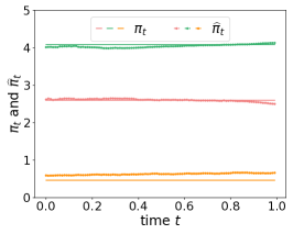
Following Lacker & Soret (2020), the analytical solution is given by

Ο€tβˆ—β‰‘Ο€βˆ—=δ​μσ2+Ξ½2βˆ’ΞΈβ€‹(Ξ΄βˆ’1)​σσ2+Ξ½2​ϕ1+ψ,ctβˆ—=(1Ξ²+(1Ξ»βˆ’1Ξ²)​eβˆ’Ξ²β€‹(Tβˆ’t))βˆ’1,formulae-sequencesubscriptsuperscriptπœ‹π‘‘superscriptπœ‹βˆ—π›Ώπœ‡superscript𝜎2superscript𝜈2πœƒπ›Ώ1𝜎superscript𝜎2superscript𝜈2italic-Ο•1πœ“subscriptsuperscript𝑐𝑑superscript1𝛽1πœ†1𝛽superscript𝑒𝛽𝑇𝑑1\displaystyle\pi^{*}_{t}\equiv\pi^{\ast}=\frac{\delta\mu}{\sigma^{2}+\nu^{2}}-\frac{\theta(\delta-1)\sigma}{\sigma^{2}+\nu^{2}}\frac{\phi}{1+\psi},\quad c^{*}_{t}=\left(\frac{1}{\beta}+(\frac{1}{\lambda}-\frac{1}{\beta})e^{-\beta(T-t)}\right)^{-1}, (D.3)

where

Ο•=𝔼​[δ​μ​σσ2+Ξ½2],ψ=𝔼​[θ​(Ξ΄βˆ’1)​σ2Οƒ2+Ξ½2],Ξ»=Ο΅βˆ’Ξ΄β€‹(e𝔼​[log⁑(Ο΅βˆ’Ξ΄)])βˆ’ΞΈβ€‹(Ξ΄βˆ’1)1+𝔼​[θ​(Ξ΄βˆ’1)],formulae-sequenceitalic-ϕ𝔼delimited-[]π›Ώπœ‡πœŽsuperscript𝜎2superscript𝜈2formulae-sequenceπœ“π”Όdelimited-[]πœƒπ›Ώ1superscript𝜎2superscript𝜎2superscript𝜈2πœ†superscriptitalic-ϡ𝛿superscriptsuperscript𝑒𝔼delimited-[]superscriptitalic-Ο΅π›Ώπœƒπ›Ώ11𝔼delimited-[]πœƒπ›Ώ1\displaystyle\phi=\mathbb{E}\left[\frac{\delta\mu\sigma}{\sigma^{2}+\nu^{2}}\right],\quad\psi=\mathbb{E}\left[\frac{\theta(\delta-1)\sigma^{2}}{\sigma^{2}+\nu^{2}}\right],\quad\lambda=\epsilon^{-\delta}\,\left(e^{\mathbb{E}\left[\log(\epsilon^{-\delta})\right]}\right)^{-\frac{\theta(\delta-1)}{1+\mathbb{E}\left[\theta(\delta-1)\right]}},
Ξ²=θ​(Ξ΄βˆ’1)​𝔼​[δ​ρ]1+𝔼​[θ​(Ξ΄βˆ’1)]βˆ’Ξ΄β€‹Ο,π›½πœƒπ›Ώ1𝔼delimited-[]π›ΏπœŒ1𝔼delimited-[]πœƒπ›Ώ1π›ΏπœŒ\displaystyle\beta=\theta(\delta-1)\frac{\mathbb{E}\left[\delta\rho\right]}{1+\mathbb{E}\left[\theta(\delta-1)\right]}-\delta\rho,

and

ρ=(1βˆ’1Ξ΄)𝜌11𝛿\displaystyle\rho=\left(1-\frac{1}{\delta}\right)\, {Ξ΄2​(Οƒ2+Ξ½2)(ΞΌβˆ’ΟƒΟ•1+ψθ(1βˆ’1Ξ΄))2+12(Ο•1+ψ)2ΞΈ2(1βˆ’1Ξ΄)\displaystyle\left\{\frac{\delta}{2(\sigma^{2}+\nu^{2})}\left(\mu-\sigma\frac{\phi}{1+\psi}\theta(1-\frac{1}{\delta})\right)^{2}+\frac{1}{2}\left(\frac{\phi}{1+\psi}\right)^{2}\theta^{2}\left(1-\frac{1}{\delta}\right)\right.
βˆ’ΞΈπ”Ό[δ​μ2βˆ’ΞΈβ€‹(Ξ΄βˆ’1)​σ​μ​ϕ1+ΟˆΟƒ2+Ξ½2]+ΞΈ2𝔼[(Ξ΄β€‹ΞΌβˆ’ΞΈβ€‹(Ξ΄βˆ’1)​σ​ϕ1+ψ)2Οƒ2+Ξ½2]}.\displaystyle-\theta\mathbb{E}\left[\frac{\delta\mu^{2}-\theta(\delta-1)\sigma\mu\frac{\phi}{1+\psi}}{\sigma^{2}+\nu^{2}}\right]+\left.\frac{\theta}{2}\mathbb{E}\left[\frac{(\delta\mu-\theta(\delta-1)\sigma\frac{\phi}{1+\psi})^{2}}{\sigma^{2}+\nu^{2}}\right]\right\}.

Note that the expression of mtsubscriptπ‘šπ‘‘m_{t}, Ξ“tsubscriptΓ𝑑\Gamma_{t} and the maximized expected utility are not given in Lacker & Soret (2020). For completeness, we give their derivations below. Since ctβˆ—subscriptsuperscript𝑐𝑑c^{*}_{t} in (D.3) doesn’t depend on the common noise B𝐡B, Ξ“t:=exp⁑𝔼​[log⁑ctβˆ—|β„±tB]assignsubscriptΓ𝑑𝔼delimited-[]conditionalsuperscriptsubscriptπ‘π‘‘βˆ—superscriptsubscriptℱ𝑑𝐡\Gamma_{t}:=\exp\mathbb{E}[\log c_{t}^{\ast}|\mathcal{F}_{t}^{B}] admits a unique formula for all agents

Ξ“t=exp⁑𝔼​[log⁑ctβˆ—].subscriptΓ𝑑𝔼delimited-[]subscriptsuperscript𝑐𝑑\Gamma_{t}=\exp\mathbb{E}[\log c^{*}_{t}].

To obtain the formula for mt:=exp⁑𝔼​[log⁑Xtβˆ—|β„±tB]assignsubscriptπ‘šπ‘‘π”Όdelimited-[]conditionalsuperscriptsubscriptπ‘‹π‘‘βˆ—superscriptsubscriptℱ𝑑𝐡m_{t}:=\exp\mathbb{E}[\log X_{t}^{\ast}|\mathcal{F}_{t}^{B}], we first deduce by Itô’s formula that

d​log⁑Xtβˆ—=Ο€tβˆ—β€‹(μ​d​t+ν​d​Wt+σ​d​Bt)βˆ’12​(2​ctβˆ—+(Ο€tβˆ—)2​σ2+(Ο€tβˆ—)2​ν2)​d​t,dsuperscriptsubscriptπ‘‹π‘‘βˆ—superscriptsubscriptπœ‹π‘‘βˆ—πœ‡dπ‘‘πœˆdsubscriptπ‘Šπ‘‘πœŽdsubscript𝐡𝑑122superscriptsubscript𝑐𝑑superscriptsuperscriptsubscriptπœ‹π‘‘βˆ—2superscript𝜎2superscriptsuperscriptsubscriptπœ‹π‘‘βˆ—2superscript𝜈2d𝑑\,\mathrm{d}\log X_{t}^{\ast}=\pi_{t}^{\ast}(\mu\,\mathrm{d}t+\nu\,\mathrm{d}W_{t}+\sigma\,\mathrm{d}B_{t})-\frac{1}{2}(2c_{t}^{*}+(\pi_{t}^{\ast})^{2}\sigma^{2}+(\pi_{t}^{\ast})^{2}\nu^{2})\,\mathrm{d}t, (D.4)

from which we easily get

𝔼​[log⁑Xtβˆ—|β„±tB]=𝔼​[log⁑ξ]+𝔼​[Ο€βˆ—β€‹ΞΌβˆ’12​(Ο€βˆ—)2​(Οƒ2+Ξ½2)]​tβˆ’βˆ«0t𝔼​[csβˆ—]​dt+Ο€βˆ—β€‹Οƒβ€‹Bt,𝔼delimited-[]conditionalsuperscriptsubscriptπ‘‹π‘‘βˆ—subscriptsuperscriptℱ𝐡𝑑𝔼delimited-[]πœ‰π”Όdelimited-[]superscriptπœ‹πœ‡12superscriptsuperscriptπœ‹2superscript𝜎2superscript𝜈2𝑑superscriptsubscript0𝑑𝔼delimited-[]subscriptsuperscript𝑐𝑠differential-d𝑑superscriptπœ‹πœŽsubscript𝐡𝑑\mathbb{E}[\log X_{t}^{\ast}|\mathcal{F}^{B}_{t}]=\mathbb{E}[\log\xi]+\mathbb{E}[\pi^{*}\mu-\frac{1}{2}(\pi^{*})^{2}(\sigma^{2}+\nu^{2})]t-\int_{0}^{t}\mathbb{E}[c^{*}_{s}]\,\mathrm{d}t+\pi^{*}\sigma B_{t},

and mt=exp⁑𝔼​[log⁑Xtβˆ—|β„±tB]subscriptπ‘šπ‘‘π”Όdelimited-[]conditionalsuperscriptsubscriptπ‘‹π‘‘βˆ—subscriptsuperscriptℱ𝐡𝑑m_{t}=\exp\mathbb{E}[\log X_{t}^{\ast}|\mathcal{F}^{B}_{t}]. The maximized expected utility of this game is given by 𝔼​[v​(0,ΞΎ,𝔼​[ΞΎ])]𝔼delimited-[]𝑣0πœ‰π”Όdelimited-[]πœ‰\mathbb{E}[v(0,\xi,\mathbb{E}[\xi])], with

v​(t,x,y)=ϡ​(1βˆ’1Ξ΄)βˆ’1​x1βˆ’1δ​yβˆ’ΞΈβ€‹(1βˆ’1Ξ΄)​f​(t),𝑣𝑑π‘₯𝑦italic-Ο΅superscript11𝛿1superscriptπ‘₯11𝛿superscriptπ‘¦πœƒ11𝛿𝑓𝑑v(t,x,y)=\epsilon\left(1-\frac{1}{\delta}\right)^{-1}x^{1-\frac{1}{\delta}}y^{-\theta(1-\frac{1}{\delta})}f(t),

and f​(t)𝑓𝑑f(t) is defined by

f​(t)=exp⁑{∫tT(ρ+1δ​csβˆ—+𝔼​[csβˆ—]​(1βˆ’1Ξ΄)​θ)​ds}.𝑓𝑑superscriptsubscriptπ‘‘π‘‡πœŒ1𝛿superscriptsubscript𝑐𝑠𝔼delimited-[]superscriptsubscript𝑐𝑠11π›Ώπœƒdifferential-d𝑠f(t)=\exp\left\{\int_{t}^{T}\left(\rho+\frac{1}{\delta}c_{s}^{*}+\mathbb{E}[c_{s}^{*}]\left(1-\frac{1}{\delta}\right)\theta\right)\,\mathrm{d}s\right\}.

Note that, to ensure the positiveness of Xtsubscript𝑋𝑑X_{t} required by using the power utility, the trajectories of Xtsubscript𝑋𝑑X_{t} are obtained by simulating log⁑Xtsubscript𝑋𝑑\log X_{t} via (D.4) then taking the exponential.

Appendix E Plots of Ο€tsubscriptπœ‹π‘‘\pi_{t}, ctsubscript𝑐𝑑c_{t}, Ξ“t=exp⁑𝔼​(log⁑ct|β„±tB)subscriptΓ𝑑𝔼conditionalsubscript𝑐𝑑subscriptsuperscriptℱ𝐡𝑑\Gamma_{t}=\exp\mathbb{E}(\log c_{t}|\mathcal{F}^{B}_{t}) for Mean-Field Game of Optimal Consumption and Investment
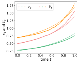
Refer to caption
(a) Ο€tsubscriptπœ‹π‘‘\pi_{t}
Refer to caption
(b) ctsubscript𝑐𝑑c_{t}
Refer to caption
(c) Ξ“t=exp⁑𝔼​(log⁑ct|β„±tB)subscriptΓ𝑑𝔼conditionalsubscript𝑐𝑑subscriptsuperscriptℱ𝐡𝑑\Gamma_{t}=\exp\mathbb{E}(\log c_{t}|\mathcal{F}^{B}_{t})
Figure 5: Plots on test data for three different (X0i,Wi,Bi,ΞΆi)superscriptsubscript𝑋0𝑖superscriptπ‘Šπ‘–superscript𝐡𝑖superscriptπœπ‘–(X_{0}^{i},W^{i},B^{i},\zeta^{i}). Solid line is the benchmark solution and dashed line is the numerical approximation using the Sig-DFP algorithm. Each panel presents three trajectories of Ο€tsubscriptπœ‹π‘‘\pi_{t}, ctsubscript𝑐𝑑c_{t}, and Ξ“t=exp⁑𝔼​(log⁑ct|β„±tB)subscriptΓ𝑑𝔼conditionalsubscript𝑐𝑑subscriptsuperscriptℱ𝐡𝑑\Gamma_{t}=\exp\mathbb{E}(\log c_{t}|\mathcal{F}^{B}_{t}) and their approximations. Parameter choices are: δ∼U​(2,2.5),μ∼U​(0.25,0.35),ν∼U​(0.2,0.4),ΞΈ,ξ∼U​(0,1),ΟƒβˆΌU​(0.2,0.4)formulae-sequencesimilar-toπ›Ώπ‘ˆ22.5formulae-sequencesimilar-toπœ‡π‘ˆ0.250.35formulae-sequencesimilar-toπœˆπ‘ˆ0.20.4πœƒformulae-sequencesimilar-toπœ‰π‘ˆ01similar-toπœŽπ‘ˆ0.20.4\delta\sim U(2,2.5),\mu\sim U(0.25,0.35),\nu\sim U(0.2,0.4),\theta,\xi\sim U(0,1),\sigma\sim U(0.2,0.4), ϡ∼U​(0.5,1)similar-toitalic-Ο΅π‘ˆ0.51\epsilon\sim U(0.5,1).

Appendix F Experiment setup for the high-dimensional case n0=5subscript𝑛05n_{0}=5

To test the performance of Sig-DFP in high dimensions, we implement a toy experiment on the mean-field game of optimal consumption and investment with the common noise of dimension n0=5subscript𝑛05n_{0}=5. Specifically, we modify the σ​d​Bt𝜎dsubscript𝐡𝑑\sigma\,\mathrm{d}B_{t} term in (5.7) to be in high dimensions, i.e., Xtsubscript𝑋𝑑X_{t} now follows

d​Xt=Ο€t​Xt​(μ​d​t+ν​d​Wt+𝝈T​d​𝑩t)βˆ’ct​Xt​d​t,dsubscript𝑋𝑑subscriptπœ‹π‘‘subscriptπ‘‹π‘‘πœ‡dπ‘‘πœˆdsubscriptπ‘Šπ‘‘superscript𝝈Tdsubscript𝑩𝑑subscript𝑐𝑑subscript𝑋𝑑d𝑑\,\mathrm{d}X_{t}=\pi_{t}X_{t}(\mu\,\mathrm{d}t+\nu\,\mathrm{d}W_{t}+{\bm{\sigma}}^{\operatorname{T}}\,\mathrm{d}{\bm{B}}_{t})-c_{t}X_{t}\,\mathrm{d}t,

where 𝝈:=(Οƒ1,…,Οƒ5)Tassign𝝈superscriptsubscript𝜎1…subscript𝜎5T{\bm{\sigma}}:=(\sigma_{1},\dots,\sigma_{5})^{\operatorname{T}}, 𝑩tsubscript𝑩𝑑{\bm{B}}_{t} is a 555-dimensional Brownian motion, and X0=ΞΎsubscript𝑋0πœ‰X_{0}=\xi. We use the same hyperparameters for training and provide the running time in TableΒ 6.