Base flow decomposition for complex moving objects in linear hydrodynamics: application to helix-shaped flagellated microswimmers

Abstract

The motion of microswimmers in complex flows is ruled by the interplay between swimmer propulsion and the dynamics induced by the fluid velocity field. Here we study the motion of a chiral microswimmer whose propulsion is provided by the spinning of a helical tail with respect to its body in a simple shear flow. Thanks to an efficient computational strategy that allowed us to simulate thousands of different trajectories, we show that the tail shape dramatically affects the swimmer’s motion. In the shear dominated regime, the swimmers carrying an elliptical helical tail show several different Jeffery-like (tumbling) trajectories depending on their initial configuration. As the propulsion torque increases, a progressive regularization of the motion is observed until, in the propulsion dominated regime, the swimmers converge to the same final trajectory independently on the initial configuration. Overall, our results show that elliptical helix swimmer presents a much richer variety of trajectories with respect to the usually studied circular helix tails.

I Introduction

Several microorganisms move in liquids thanks to rotating flagella. For instance, the bacterium Escherichia coli has several flagella that form a rotating helical bundle berg2008coli , while other bacteria, like Pseudomonas aeruginosa, exploit the same propulsion strategy but using a single helical flagellum qian2013bacterial ; sartori2018wall . The high swimming speed and the relatively simple geometry of such a kind of chiral microswimmers make them suitable for various applications and, in the last decade, artificial versions of flagellated microswimmers have been proposed for micromanipulation zhang2010artificial and drug delivery mhanna2014artificial .

The interaction between helical flagellated microswimmers and the environment presents a rich behavior that has received extensive attention in the past decades lauga2009hydrodynamics ; elgeti2015physics . Close to interfaces, helical flagellated microswimmers follow circular trajectories that are clockwise for solid walls lauga2006swimming ; guccione2017diffusivity ; shum2010modelling and counterclockwise for liquid-air interfaces di2011swimming ; pimponi2016hydrodynamics ; hu2015physical ; bianchi20193d . Far from the wall, the hydrodynamic of active microorganisms is highly affected by the local flow conditions. A relevant phenomenon is rheotaxis, i.e. the movement resulting from fluid velocity gradients. As shown by Fu et al. fu2012bacterial , the rheotaxis of flagellated microswimmers with helical tail is a purely physical phenomenon due to interplay between velocity gradients and the shape of chiral flagella. Indeed, for a passive helix, the shear induces Jeffery-like tumbling motion parallel to the shear plane fu2009separation . Along the orbit, elongated helices spend more time aligned with streamlines. Since this configuration is not symmetric with respect to the shear plane, a chirality-dependent drift generally sets in. For active helical microswimmer, the passive chirality-induced drift is often overwhelmed by the propulsion: the shear results in a preferential orientation of the swimmers along which, thanks to the self-propulsion, the swimmer moves fu2012bacterial ; rusconi2014bacterial . Hence, the swimming direction is ruled by the shear, likely preventing the possibility of controlling the orientation of microswimmers in an assigned flow fu2012bacterial .

A way to escape from the monotonous rheotaxis in shear flow is to increase the number of degrees of freedom (DOF) of the microswimmers, for instance employing multiple tails kanehl2014fluid , or adaptively changing the angle between body and tail(s) riley2018swimming . The existence of external flexibility, however, complicates the control of microswimmers particularly in view of possible technological applications. Another possibility to escape from the rheotaxis is to break some symmetries of the swimmer geometry. In this aspect, interestingly, it has recently been shown that the change of the cross-section of the ellipsoids from circle to ellipse can lead to chaotic orbits einarsson2016tumbling ; einarsson2015angular ; thorp2019motion .

Inspired by this phenomenon, we numerically analyzed the dynamics of a microswimmer made by an axisymmetric body and by an elliptical helix, (i.e. a helix that lies on an elliptical cylinder) in a shear flow. The possible presence of a large variety of different trajectories, requires a systematic exploration of a large number of initial conditions. This, in turn, pushed us to develop and apply an accurate and fast computational approach based on a decomposition of dynamics in an active and a passive motion that allowed to speed-up the simulations and to collect, for each case, thousands of trajectories. Our results show that the elliptical helix swimmer presents a much richer variety of possible trajectories with respect to the well studied circular helix tails. In particular, we found for an elliptical helical tail a much higher spinning frequency is needed to control the asymptotic swimming regime.

II Set-up and Method

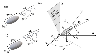
Figure 1: Sketch of microswimmer locomotion in a shear flow. The microswimmer body is a prolate ellipsoid of major axis $r_{h1}$ and minor axis $r_{h2}$. In model I (a), the tail is a circular helix, i.e. a helix built on a circular cylinder of radius $r_{t1}$, while in model II (b), the tail is an elliptical helix, i.e. a helix built on an elliptical cylinder of radii $r_{t1}$ and $r_{t2}=3r_{t1}$. (c) The shear flow is in the $\textbf{X}_{1}\textbf{X}_{3}$ plane of the global coordinate frame $\textbf{O}\textbf{X}_{1}\textbf{X}_{2}\textbf{X}_{3}$. A body coordinate frame $\textbf{O}\bm{{}^{\prime}}\textbf{e}_{1}\textbf{e}_{2}\textbf{e}_{3}$ moves with the swimmer body. The polar $\theta$ azimuthal $\phi$ and rotation $\psi$ angles are used to describe the orientation of the body frame with respect to the global frame. Moreover, we also define the angle between the swimmer axis $\bm{p}=\textbf{e}_{3}$ and $\textbf{X}_{2}$ as $\eta=\arccos(\sin\theta\sin\phi)$. The tail rotates with respect to the $\textbf{e}_{3}$ so that each point of the rigid tail describes a circle in the plane $\textbf{e}_{2}\textbf{e}_{3}$, with $\psi_{t}$ the corresponding rotation angle. The motion of the microswimmer body is completely defined when the translational velocity $\bm{U}$ of the body center, the body rotational velocity $\bm{\Omega}$ and the tail spinning $\Omega_{t}=\dot{\psi_{t}}$ are given.

Two kinds of microswimmers are compared in this study: one with a circular helical tail, i.e. a helix that lies on a circular cylinder (model I) and one with an elliptical helical tail, i.e. a helix that lies on a cylinder of elliptical section (model II), see Fig. 1. For both models, the body is a prolate ellipsoid of radii $r_{h1}$ and $r_{h2}$, the center of the body is indicated as $\bm{x}_{c}$. A body coordinate frame $\textbf{O}\bm{{}^{\prime}}\textbf{e}_{1}\textbf{e}_{2}\textbf{e}_{3}$ with origin at $\bm{x}_{c}$ and $\textbf{e}_{3}$ oriented as the major ellipsoid axis is defined. Concerning the tail, its centerline follows the helix equation in the body coordinate frame

$${\bm{r}}=(r_{t1}\cos(2\pi s),r_{t2}\sin(2\pi s),\lambda s-\delta_{bt})\,,$$ (1)

where $s\in[-n/2,n/2]$ with $n$ the number of periods of the tail, $\delta_{bt}$ is the distance from $\bm{x}_{c}$ to the tail center, $\lambda$ is the pitch of the helix and $r_{t1}$ and $r_{t2}$ are the radius of the elliptical cylinder on which the helix lies. For circular helix, $r_{t1}=r_{t2}$, while for elliptical helix, $r_{t1}=3r_{t2}$. The flagellum section is a cylinder of radius $\rho_{t}$. All the details of the swimmer geometry are reported in the appendix A.

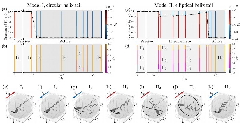
Figure 2: Microswimmer motion in a simple shear flow. For each case, from $10^{3}$ to $10^{4}$ simulations with different initial conditions were run. Panel a) reports the fraction of the circular helix swimmers that have a drift velocity oriented as $\textbf{X}_{2}$ ($U_{2}>0$). The bars in panel a) indicate the lateral velocity $U_{2}$ for the different initial conditions while the bars in panel b) refer to the normalized average angle $\langle\eta/\pi\rangle$ between $\textbf{X}_{2}$ and the microswimmer head orientation $\bm{p}$. In the passive regime, all the trajectories converge to the same final state ($\mathrm{I_{1}}$, panel e) where the swimmer is oriented as $-\textbf{X}_{2}$ while its velocity is $U_{2}\cong 10^{-4}$. In the active regime, the swimmer is again oriented as $-\textbf{X}_{2}$, but $U_{2}<0$, see configuration $\mathrm{I_{2}}$ (f) and $\mathrm{I_{3}}$ (g). The dot-dashed line corresponds to the fraction of swimmers for which $U_{2}>0$. Panel $(c)$ and $(d)$ refer to velocity $U_{2}$ and orientation $\langle\eta/\pi\rangle$ for elliptical helix tail. Here, a new intermediate regime appears between the active and passive regime. In this intermediate regime, both positive and negative drift velocities $U_{2}$ are possible. Panels (e)-(k) report examples of the swimmer Jeffery-like tumbling motion (shear in the $X1X3$ plane). The solid lines on the spheres represent the direction of the swimmer axis $\bm{p}$ along one period while the red and blue arrows refer to the direction of the average velocity along $X_{2}$.

The microswimmer has 7 degree of freedoms (DOFs): 3 translation DOFs $\bm{x}_{c}=(x_{c1},x_{c2},x_{c3})$, 3 rotational DOFs $\bm{\theta}_{c}=(\theta,\phi,\psi)$ plus the tail orientation $\phi_{t}$ with respect to the body. The body orientation is defined by the unit vector $\bm{p}=(\sin\theta\cos\phi,\sin\theta\sin\phi,\cos\theta)$ here expressed as a function of the polar $\theta$ and the azimuthal $\phi$ angles. It is also instrumental to define the angle $\eta=\arccos(\sin\theta\sin\phi)$ between $\bm{p}$ and $\textbf{X}_{2}$, see Fig. 1. The value $\eta=0$ ($\eta=\pi$) corresponds to a configuration where the microswimmer is perpendicular to the shear plane and points toward positive (negative) $\textbf{X}_{2}$, while $\eta=0.5\pi$ corresponds to the microswimmer lying in the shear plane. The swimmer body moves with translational velocity $\bm{U}$ and rotational velocity $\bm{\Omega}$ while the tail spins at a constant speed and consequently $\Omega_{t}=\dot{\psi_{t}}$.

The governing equations of fluid velocity $\bm{u}$ and pressure $p$ fields are the Stokes equations

$$\nabla\cdot\bm{u} =0\,,$$ (2)

$$\mu\nabla^{2}\bm{u} =\nabla p\,,$$ (3)

with $\mu$ the fluid viscosity. The no-slip boundary condition is applied on the surfaces of the head

$$\bm{u}(\bm{x}) =\bm{U}+\bm{\Omega}\times\bm{r}\,,$$ (4)

and of the tail of the microswimmer

$$\bm{u}(\bm{x}) =\bm{U}+(\bm{\Omega}+\Omega_{t}\bm{p})\times\bm{r}\,,$$ (5)

where in both equations $\bm{r}$ indicates the relative position of the boundary point with respect to the center of the swimmer head $\bm{x}_{c}$. Note that, in general, $\bm{U}$ and $\bm{\Omega}$ are not parallel to the swimmer orientation $\bm{p}$. Thus, there exists no simple relation between the active spin $\Omega_{t}$ and the velocities $(\bm{U},\bm{\Omega})$.

The method for the solution of the swimming problem is briefly sketched in the following while details are reported in the appendix A. The fundamental step is to get the swimmer generalized velocity $(\bm{U},\bm{\Omega})$ as a function of the swimmer configuration and tail spinning velocity $\Omega_{t}$. Once $(\bm{U},\bm{\Omega})$ are known, the standard rigid body kinematic equations can be solved for the swimmer head. The swimming problem is solved by decoupling the $(\bm{U},\bm{\Omega})$ into two parts where the active part $(\bm{U}_{a},\bm{\Omega}_{a})$ corresponds to the movement of the microswimmer in a bulk fluid at rest while the passive part $(\bm{U}_{p},\bm{\Omega}_{p})$ corresponds to a passive swimmer ($\Omega_{t}=0$) immersed in the external flow field $\bm{u}_{b}$. Thanks to the linearity, the active part can be expressed as $\bm{U}_{a}=\Omega_{t}\bm{R}\tilde{\bm{U}}_{a}$ , $\bm{\Omega}_{a}=\Omega_{t}\bm{R}\tilde{\bm{\Omega}}_{a}$ where $\bm{R}$ is the rotation matrix that transforms the expression of a vector in the body reference frame into its expression in the global reference frame and $(\tilde{\bm{U}}_{a},\tilde{\bm{\Omega}}_{a})$ are the velocities for a microswimmer swimming with $\omega_{t}=1$ in a configuration where body and global frame coincides. Concerning the passive part, instead, we exploit the local decomposition of $\bm{u}_{b}$ in three components, a rigid translation at $\bm{x}_{c}$, a rigid rotation $\bm{\omega}_{p}^{S}$ (associated to antisymmetric part of the velocity gradient $S_{ij}$) and a deviatoric part (symmetric part of the velocity gradient $E_{ij}$). The deviatoric part $E_{ij}$ can be further decomposed into five components. For each of them, we can solve a swimming problem and get the contributions to the swimmer translational $\bm{U}$ and angular $\bm{\Omega}$ velocities. Combining all those contributions, the microswimmer velocity in an external flow is obtained as

$$\bm{U} =\Omega_{t}\bm{R}\tilde{\bm{U}}_{a}+\bm{U}_{p}^{b}+\bm{R}\sum_{k=1}^{5}\tilde{\beta}_{k}\tilde{\bm{U}}_{k}^{E}\,,$$ (6)

$$\bm{\Omega} =\Omega_{t}\bm{R}\tilde{\bm{\Omega}}_{a}+\bm{\Omega}_{p}^{S}+\bm{R}\sum_{k=1}^{5}\tilde{\beta}_{k}\tilde{\bm{\Omega}}_{k}^{E}\,.$$ (7)

where the first term on the right hand side is the active contribution, the second term is the uniform translation $\bm{U}_{p}^{b}$ and rotation $\bm{\Omega}_{p}^{S}$ due to the external flow and the last terms are the five contribution due to the deviatoric part of the velocity gradient. The weights $\tilde{\beta}_{k}$ depends only on $\bm{u}_{b}$ and on the swimmer orientations, details are reported in the appendix A. It is worth noting that, as a first approximation, a more appropriate model for the head-tail coupling is to fix the exchanged torque berg1993torque ; xing2006torque . However, in our case, the head-tail coupling enters only in the active part of Eqs.(6)-(7). Since the active part corresponds to the movement of the microswimmer in a bulk fluid at rest, the tail spin $\Omega_{t}$ is proportional to the motor torque and, hence, considering a fixed spin or a fixed torque only amounts to a linear rescaling with no effect on the observed phenomenology.

The main advantage of the proposed method is that only six solutions of the swimming problem are needed; one for $(\tilde{\bm{U}}_{a},\tilde{\bm{\Omega}}_{a})$ and five for $(\tilde{\bm{u}}_{k}^{E},\tilde{\bm{\Omega}}_{k}^{E})$. These swimming problems can be solved with any Stokes solver. Here we use the method of fundamental solution (MFS) young2006method that is summarized in the appendix A. Once these solutions are known, one can integrate the rigid body kinematics to get the swimmer trajectory. Here, this integration step is performed using a quaternion formulation and a $4^{th}$ order Runge-Kutta method.

III Results

In this study, the microswimmer is immersed in an unbounded shear flow

$$\bm{u}_{b} =(x_{3}\tau_{s},0,0)\,.$$ (8)

Without loss of generality, we select as time unit $1/\tau_{s}$ and as length unit of length $r_{h1}$ the larger axis of the ellipse. Due to the linearity of the problem, the spin $\Omega_{t}$ is the only crucial parameter for given microswimmer. For both the circular (model I) and the elliptical (model II) helical tail microswimmers, we studied the motions at different tail spinning velocity $\Omega_{t}$. For each $\Omega_{t}$, we simulated from $10^{3}$ to $10^{4}$ trajectories starting from different initial conditions with random orientation. The center of the head is initially placed in the origin at $t=0$. In all the cases, after a transient, the swimmer orientation converges to periodic trajectories. Concerning the swimmer translation, different scenarios are possible depending on the swimmer tail geometry, its spinning velocity $\Omega_{t}$ and its initial condition. A summary of the different possibilities is reported in figure 2 and discussed in the following sections.

III.1 Circular helix

For the circular helix swimmer, in the passive case (tail spinning velocity $\Omega_{t}=0$) after a transient, the swimmer is always oriented along $-\textbf{X}_{2}$, i.e. normally to the shear plane $\textbf{X}_{1}\textbf{X}_{3}$, and it moves along $\textbf{X}_{2}$, i.e. $U_{2}>0$. In the Figure 2a, those information are condensed in panel a) where the fraction of the trajectories that result in final drift $U_{2}>0$ can be read on the left axes while the colored bars indicate the actual value of $U_{2}$. For instance, the orange bar at $\Omega_{t}=0$ means that all the $10^{3}$ initial conditions result in a slightly positive terminal velocity $U_{2}\cong 1.01\times 10^{-4}$ while the blue bar at $\Omega_{t}=0.015$ indicates that almost all the swimmers reach a final velocity $U_{2}\cong-3.00\times 10^{-6}$. Fig. 2b, instead, reports the orientation $\eta$ averaged on a period. For the pure passive case, $\Omega_{t}=0$, we always get $\langle\eta\rangle\cong\pi$, i.e. the swimmer is oriented perpendicularly to the shear plane. This passive swimmer regime is indicated as $\mathrm{I_{1}}$ and a sketch of its periodic orbits is reported in Fig. 2e and in Video SM1 . This result is in agreement with the shear-induced separation of pure circular helix discussed in fu2012bacterial where it was shown that microswimmers point perpendicularly to the shear plane in the direction here indicated as $-X_{2}$. A similar behavior is also observed for low spinning velocity, $\Omega_{t}<0.015$.

A further increase of the tail spinning results in a first change in the dynamics. The average orientation of the swimmer is the same, $\langle\eta\rangle\cong\pi$, but now the drift velocity is positive, $U_{2}>0$, $\mathrm{I_{2}}$ Fig. 2f. This is expected, indeed, as $\Omega_{t}$ increases, the swimmer propulsion becomes more relevant until, finally, it dominates over the passive drift induced by the shear. Interestingly, in some intervals of the spinning speed, an additional kinematics appears, $\mathrm{I_{3}}$ Fig. 2g. The swimmer undergoes to a Jeffery-like motion with $\langle\eta\rangle\in[0.8,0.9]\pi$. This motion is characterized by a slightly smaller value of the average velocity $U_{2}$. Depending on the initial condition, some trajectories converge to a motion of the $\mathrm{I_{2}}$ kind and others to $\mathrm{I_{3}}$. Overall, those data indicate that the shear always orients the swimmer along $-\textbf{X}_{2}$. For small tail spinning (passive case) the shear dominates the dynamics and the swimmer moves in the $\textbf{X}_{2}$ direction while, for large tail spinning (active case), the self-propulsion dominates and the swimmer moves in the $-\textbf{X}_{2}$ direction.

III.2 Elliptical helix

A much richer scenario occurs for swimmers with an elliptical helix tail, model II, Fig. 2c. In the passive case, we observed three main different periodic trajectories. The overall drift is positive $U_{2}>0$ in this region, as for model I. The average orientation $\langle\eta/\pi\rangle$, however, is significantly different. The first kind of trajectory $\mathrm{II_{1}}$ orientates along $-\textbf{X}_{2}$ as for model I. The other two kinds of trajectories, $\mathrm{II_{2}}$ and $\mathrm{II_{3}}$, present Jeffery-like tumbling behaviors that differ from $\mathrm{II_{1}}$, see Fig 2h-j and Video SM2, SM3 and SM4 Note1 . In particular, for $\mathrm{II_{3}}$ we observe that the tumbling occours almost in the shear plane. Similar to the shear induced separation of pure helix fu2009separation , such kind of tumbling (Jeffery-like) motion on the shear plane is associated to a lateral velocity ($U_{2}$) of the microswimmer that, in our case, it is larger than the one corresponding to $\mathrm{II_{1}}$, see Fig. 2c. No simple rules are found to associate the final microswimmer trajectory to its initial orientation, see Supplementary Section S1   where examples of the time evolution of the orientation $\bf p$ are reported together with a diagram representing the domains in the orientation space that led to $\mathrm{II_{1}}$, $\mathrm{II_{2}}$, $\mathrm{II_{3}}$ trajectories.

As spinning speed $\Omega_{t}$ increases, the system undergoes a gradual regularization. We still observe three different kinds of trajectory but the values of the average orientation $\langle\eta/\pi\rangle$ of $\mathrm{II_{1}}$, $\mathrm{II_{2}}$ and $\mathrm{II_{3}}$ get closer, until they merge. In this intermediate regime, trajectory $\mathrm{II_{1}}$ switch from positive to negative $U_{2}$ and, for this reason, we renamed it as $\mathrm{II_{4}}$, Fig. 2l. Further increases in $\Omega_{t}$ brings the system to a fully active regime where only $\mathrm{II_{4}}$ trajectory is observed: the swimmer is oriented along $-\textbf{X}_{2}$ with $U_{2}<0$. This regime is analogous to the active regime for circular helical tail, $\mathrm{I_{2}}$ trajectory.

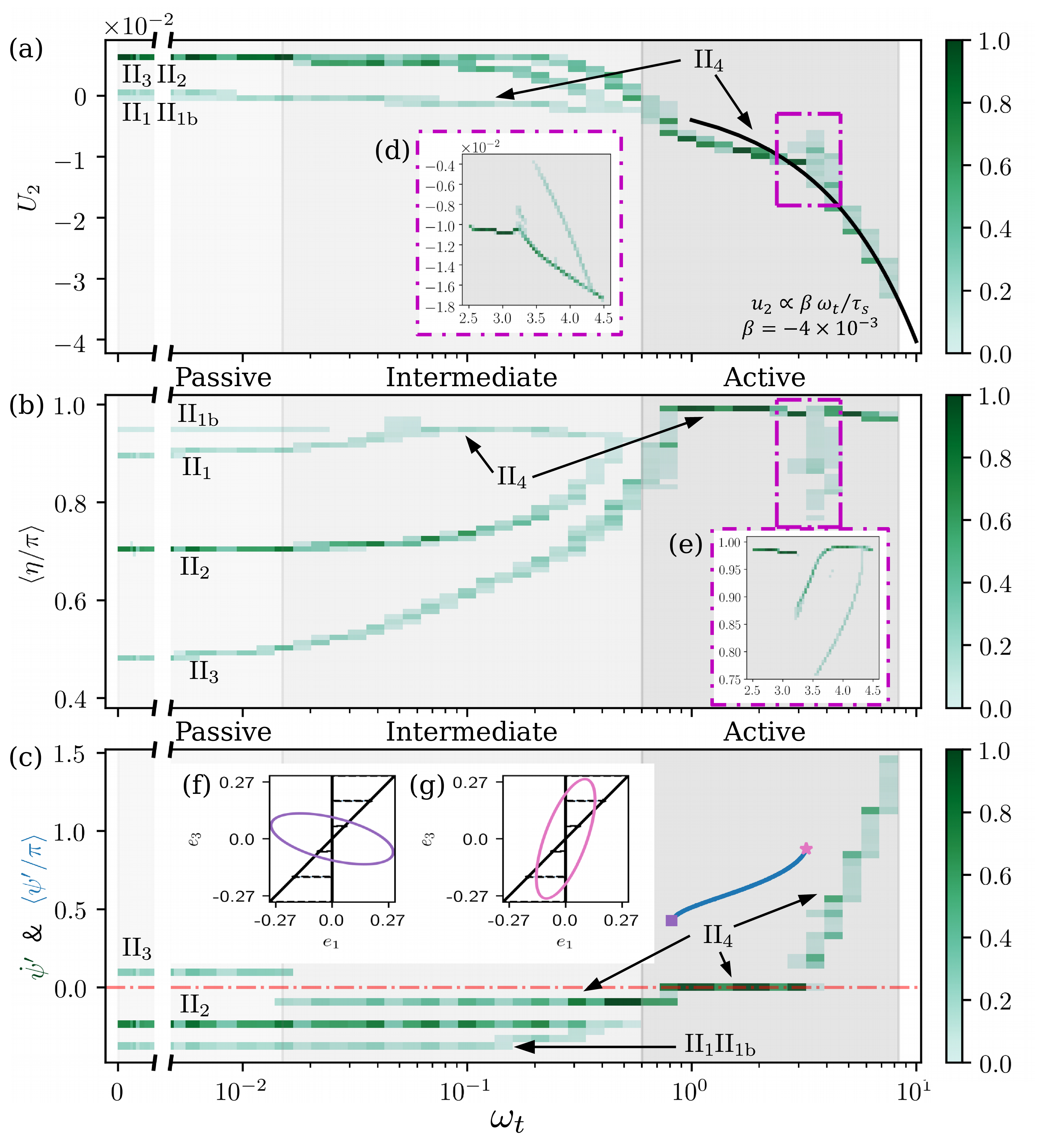
Figure 3: Elliptical helix tail microswimmer. Lateral velocity $U_{2}$ (a), normalized average angle $\langle\eta/\pi\rangle$ (b) and the absolute tail spin $\dot{\psi}^{\prime}=\dot{\psi}+\dot{\psi}_{t}$ (c) as functions of $\Omega_{t}$. Results refer to $450$ trajectories for each $\Omega_{t}$. The green color scale indicates the probability that one initial condition converges to the corresponding value on the vertical axis, for instance, in the passive case, almost $~{}75\%$ of the swimmers converge to the trajectory $\mathrm{II}_{2}$ that corresponds to $\langle\eta\rangle\cong 0.7\pi$ (dark green). Black solid line in panel (a) is the velocity of the same microswimmer in a fluid at rest. Panels (d) and (e) report a detailed view of the regions enclosed by the violet dotted boxes. The freezing tail phenomenon discussed in the text is sketched in panels (f) and (g) while the corresponding average $\psi^{\prime}$ is reported as a solid blue line between $0.8<\Omega_{t}<3.2$ in panel (c).

To better characterize the elliptical helical tail microswimmer, we performed additional simulations that allowed us to observe further details of the swimmer motion. Results are reported in Fig. 3a for the lateral velocity $U_{2}$ and in Fig. 3b for the normalized average angle $\langle\eta/\pi\rangle$. For each $\Omega_{t}$ we performed 450 simulations with random initial orientation. The green color scale corresponds to the probability that the swimmers reach a steady state with the corresponding value of $U_{2}$ and $\langle\eta/\pi\rangle$. For instance, at low $\Omega_{t}$ (passive regime), four kinds of stable trajectories exist. Three of them, $\mathrm{II}_{1},\mathrm{II}_{2},\mathrm{II}_{3}$, were already discussed in Fig. 2. The last one, indicated as $\mathrm{II}_{1b}$, corresponding to $\langle\eta\rangle\sim 0.95\pi$, is quite rare (light green in Fig. 3b) and very similar to $\mathrm{II}_{1}$. As already discussed in Fig 2, the trajectories oriented perpendicularly to the shear plane ($\mathrm{II}_{1}$ and $\mathrm{II}_{1b}$ for which $\langle\eta\rangle\in[0.9,1]\pi$) have almost no lateral motion ($U_{2}\cong 0$). In contrast, the other two kinds of trajectories, characterized by Jeffery-like tumbling close to the shear plane ($\mathrm{II}_{2}$ and $\mathrm{II}_{3}$), show a significant lateral motion, $U_{2}>0$, see also Fig. 2i and Fig. 2j. Moreover, Fig. 3 also better evidences how, through increasing of tail spin $\Omega_{t}$, the tumbling trajectories $\mathrm{II}_{2}$ and $\mathrm{II}_{3}$ progressively converge towards the $-X_{2}$ axes as apparent from the increase of $\langle\eta/\pi\rangle$. Finally, in the active regime, all the trajectories merge into a single kind where the swimmer is oriented normal to the shear plane $\langle\eta\rangle\cong\pi$.

III.3 Freezing spin

Nevertheless, some islands of complexity persist in this active region. For instance, the microswimmer is frozen by the shear flow for spinning $0.8<\Omega_{t}<3.2$. The tail of the microswimmer, when seen from the global reference frame, does not spin along the swimmer axis $\bm{p}$. This is apparent in Fig. 3c where the time derivative of the angle $\psi^{\prime}$ is reported. In essence, the tail rotates with respect to the head ($\dot{\psi}_{t}=\Omega_{t}$ is imposed in our model) but the rotation of the head with respect to the global reference frame exactly counter balances the spinning ($\psi^{\prime}=\psi+\psi_{t}$, $\dot{\psi}^{\prime}=\dot{\psi}+\dot{\psi}_{t}$, hence, $\dot{\psi}^{\prime}=0\Rightarrow\dot{\psi}=-\dot{\psi}_{t}$), see Supporting video SM5 Note1 . This is a peculiar behavior that occurs only for the elliptical helical tail and not for the circular one and it represents a further indication that slight changes in the swimmer geometry may lead to new phenomena. In fact, the tail of the microswimmer experiences a propulsion torque due to propulsion as well as a shear torque due to local velocity gradient. The balance between the two torques on the tail leads to the freezing. For the lowest spinning velocity for which the freezing occurs, i.e. $\Omega_{t}=0.81$, the propulsion torque is small. Thus, the mayor axis of the tail section is almost parallel to the shear velocity direction and, consequently, the torque induced by the shear on the tail is small, as in Fig. 3f. As the tail spinning $\Omega_{t}$ increases, the propulsion torque increases and the new balance is found for larger values of $\psi^{\prime}$. The maximum shear torque is achieved when the mayor axis of the tail section is vertical and, indeed, the last value of $\Omega_{t}=3.24$ for which this tails freezing occur corresponds to $\psi^{\prime}\approx\pi$, see Fig. 3g.

Another unexpected behavior occurs for $\Omega_{t}\in(3,4.5)$ where we observe that, again, the swimmer may converge towards multiple different trajectories, see Fig. 3d and Fig. 3e. All these trajectories have a negative $U_{2}$ and their oscillation around $\textbf{X}_{2}$ axis is limited, $\langle\eta/\pi\rangle>0.7$. For these reasons they can be overall classified as $\mathrm{II_{4}}$. Only after this last region of complexity, the motion gets finally regularized. In this fully active regime, the final swimmer speed is linear in the tail spinning, $U_{2}=\beta\Omega_{t}$, with $\beta=-4.02\times 10^{-3}$. This is expected, indeed, when the tail spin is large, the final swimmer speed is dominated by the propulsion. Indeed, the value of $\beta$ we observed is the same as we got in a simulation of the active swimmer moving in a fluid at rest represented as a black solid line in Fig. 3a. In essence, in the active regime, the shear selects the swimmer orientation, and the final speed is controlled by the tail spin. In the active regime, the swimmer dynamics is predictable and controllable: any initial condition results in the same final trajectory.

IV Conclusion

In this manuscript, we proposed an efficient computational method for the analysis of microswimmer motion in external flows. We applied our method for the analysis of microswimmers whose propulsion is due to the spinning of a flagellum (E.coli-like swimmers). Once the swimmer geometry is selected, the entire range of spinning speed of the tail can be explored by solving only six swimming problems. This allowed us to simulate thousands of different trajectories. We compared the motions of two different swimmers, one carrying a circular helical tail, i.e. a helix that lies on a circular cylinder, that is the typical geometry studied in previous theoretical and computational works, and another one carrying an elliptical helical tail. The alteration of the tail shape from circular helix to elliptical helix gives rise to a much richer scenario where different tumbling (Jeffery-like) trajectories can be observed under the same external flow condition and for the same tail spinning speed. As the propulsion torque increases, a progressive regularization of the motion is observed until, in the propulsion dominated regime, the swimmers converge to the same final trajectory for all the initial configurations. These results may have some implications on the biology of microorganisms that exploit this propulsion mechanism. Indeed, the complex Jeffery-like tumbling we observed in the shear dominated regime may provide an alternative way to increase the capability of a microswimmer to explore the space that may cooperate with the well known run and tumble motion berg2000motile . On the other hand, the high sensitivity to the shape of the tail implies that the microorganism must reach a larger spinning frequency in order to have a full control of its asymptotic swimming direction. As a result, the presence of more that one steady state also has to be carefully taken into account when designing artificial microswimmers whose motion in external flows needs to be controlled.

Appendix A Details on the methods

In this appendix, we discuss the approach we employed for the solution of the swimming problem for an active microswimmer with a single intrinsic degree of freedom (DOF) swimming in an external flow. The DOF is the spin of the tail with respect to the microswimmer body. This model can be easily extended to multiple DOFs. Our method is a combination of known approaches for solution of the Stokes equation that, for completeness, are reported in the following sections. The crucial idea it to decompose the rate of strain in five base components. This allows to reduce the solution of the swimming problem to six solutions of the Stokes equation, one for the active propulsion and five for the passive one. These swimming problems can be solved with any Stokes solver. Here we employed the method of fundamental solution (MFS) young2006method Before entering in the details of our formulation, we briefly mention some alternative approaches for the swimming problem.

Modeling the motion of a microswimmer using multiple rigid bodies is a relatively common approach (see, e.g. shum2010modelling ; pimponi2016hydrodynamics ). A key to calculate the trajectory of a microswimmer is to compute the generalized velocity $(\bm{U},\bm{\Omega})$, that can be calculated solving the Stokes equations plus the force- and torque-free conditions elgeti2015physics . The boundary element method is commonly used for Stokes equations shum2010modelling ; liu2014propulsion , although the solving method can be replaced by other formulations, such as the method of regularized Stokeslets rorai2019limitations ; cortez2005method ; zhang2020active , the boundary integral method klaseboer2012non , and the spectral boundary element method muldowney1995spectral . Since usually it is computationally expensive to calculate the generalized velocity $(\bm{U},\bm{\Omega})$ directly using full solution of the Stokes equation, several approximate theories were developed for rigid body motion in Stokes flows. Following Marcos et. al. work fu2009separation ; fu2012bacterial , Mathijssen et. al. mathijssen2019oscillatory developed an approximate formulation of an ideal chiral object using the resistive force theory that allowed to study bacteria rheotaxis close to a surface. Another alternative approach is to calculate the generalized mobility matrix of the system kim1991microhydrodynamics . For a three sphere swimmer model najafi2004simple , a quadrupole order accurate multipole expansion was recently employed to study the swimmer kinematics close to a wall under a shear flow daddi2020tuning . The possibility to extend this promising approach to more complex swimmer geometries is, however, an open issue.

A.1 Fundamental solution of Stokes equation

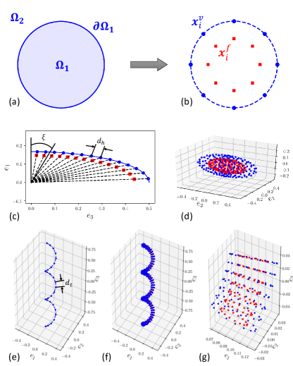
Figure 4: Sketch of the method of fundamental solutions. (a) A solid body (domain $\Omega_{1}$) moves in a bulk fluid (domain $\Omega_{2}$). The solid blue line $\partial\Omega_{1}$ is the boundary of the solid body. Boundary points $\bm{x}_{i}^{v}$ (blue circles) are selected on $\partial\Omega_{1}$ while source points, $\bm{x}_{i}^{f}$ (red squares) are placed inside the solid body. Panel (c) shows the discretization used for a quarter of an ellipse while the swimmer head is in the panel (d). Panel (e) reports the tail centerline while panel (f) refers to the discretization of the swimmer tail. Each section of the tail is modelled as a circle where, again, red squares correspond to force sources and blue circles to the boundary. In panel (g) a short section of the swimmer tail is shown.

Here, we briefly summarize the method of fundamental solution (MFS) young2006method . In the creeping flow limit, the governing equation for the fluid velocity $\bm{u}$ and pressure $p$ due to a point force singularity of strength $\bm{f}$ applied to the point $\bm{x}_{f}$ is the Stokes equations

$$\nabla\cdot\bm{u} =0\,,$$ (9)

$$\mu\nabla^{2}\bm{u} =\nabla p-\bm{f}(\bm{x}_{f})\delta(\bm{x}-\bm{x}_{f})\,,$$ (10)

where $\mu$ the fluid viscosity, and $\delta$ is the Dirac delta function. The solution of (9)-(10) (also knows as Stokeslet) reads

$$\bm{u}(\bm{x})=\bm{S}(\bm{x}_{f},\bm{x})\bm{f}(\bm{x}_{f})\,,$$ (11)

with

$$\bm{S}(\bm{x}_{f},\bm{x})=\frac{1}{8\pi\mu}\left(\frac{\textbf{I}}{r}+\frac{(\bm{x}_{f}-\bm{x})(\bm{x}_{f}-\bm{x})}{r^{3}}\right)\,,$$ (12)

where I is the unit matrix, and $r=\left\lVert\bm{x}_{f}-\bm{x}\right\rVert$. The tensor $\bm{S}(\bm{x}_{f},\bm{x})$ is commonly indicated as Oseen tensor.

The MFS young2006method was already successful employed in microfluidics, see e.g. aboelkassem2013stokeslets ; lockerby2016fundamental . In brief, as is shown in Fig. 4 (a, b), for problems where the velocity is assigned on the boundary of a solid domain $\Omega_{1}$ and the velocity field needs to determined in the external domain $\Omega_{2}$, the key of the MFS is to find an approximation field $\bm{u^{\prime}}$ that is defined in the domain $\Omega_{1}\cup\Omega_{2}$ and that fulfills the boundary condition at the frontier of $\Omega_{1}$. The fluid velocity field $\bm{u^{\prime}}$ is a smooth field that is defined in both the domains $\Omega_{1}$ and $\Omega_{2}$. A set of $n$ boundary points $\bm{x}_{i}^{v}$ located at the boundary $\partial\Omega_{1}$ are selected. For each one of them, we know its corresponding velocity $\bm{u}(\bm{x}_{i}^{v})$ from boundary conditions. A set of $n$ point forces are placed inside the domain $\Omega_{1}$ close to the boundary points, the location of the point forces being indicated as $\bm{x}_{i}^{f}$. Hence, the velocity $\bm{u}(\bm{x}_{i}^{v})$ can be expressed as

$$\begin{bmatrix}\bm{u}(\bm{x}_{1}^{v})\\ \ldots\\ \bm{u}(\bm{x}_{n}^{v})\end{bmatrix}=\begin{bmatrix}\bm{S}(\bm{x}_{1}^{f},\bm{x}_{1}^{v})&\ldots&\bm{S}(\bm{x}_{n}^{f},\bm{x}_{n}^{v})\\ &\ddots&\\ \bm{S}(\bm{x}_{1}^{f},\bm{x}_{1}^{v})&\ldots&\bm{S}(\bm{x}_{n}^{f},\bm{x}_{n}^{v})\\ \end{bmatrix}\begin{bmatrix}\bm{f}(\bm{x}_{1}^{f})\\ \ldots\\ \bm{f}(\bm{x}_{n}^{f})\end{bmatrix}\,.$$ (13)

This system has $3n$ unknowns and $3n$ equations. Once (13) is solved for $\bm{f}$, the approximated velocity $\bm{u^{\prime}}$ in a generic point $\bm{x}$ of the domain $\Omega_{1}\cup\Omega_{2}$ can be calculated as

$$\bm{u^{\prime}}(\bm{x})=\sum_{i=1}^{n}\bm{S}(\bm{x}_{i}^{f},\bm{x})\bm{f}(\bm{x}_{i}^{f})\,.$$ (14)

In the following, to simplify the notation, we will use the same symbol $\bm{u}$ for the approximated velocity and the true solutions of the Stokes problem.

A.2 The discretization of the microswimmer

A technical issue in MFS concerns the location $\bm{x}_{i}^{f}$ of the point sources. Our swimmer is composed by a spheroidal head and a helical tail. Concerning the head, we first placed the boundary point on a 2D ellipse with semi-axes $r_{h1}$ and $r_{h2}$ lying on the $\textbf{e}_{3}\textbf{e}_{1}$ plane, approximately at the same distance $d_{h}$, Andy2020 , see Fig. 4(c). The ellipsoid is a body of revolution. Hence, we rotated each point around the major axis $\textbf{e}_{3}$ of the ellipsoid obtaining a circle perpendicular to $\textbf{e}_{1}$. This circle is divided into boundary points with equal distance $d_{h}$. In this study, we select $d_{h}/r_{h1}\cong 0.047$ for a total of $1653$ boundary points lying on the swimmer head and indicated as $\bm{x}_{i}^{vh}$.

For each boundary point $\bm{x}_{i}^{vh}$, a point force is located inside the ellipsoid on the lines that connect $\bm{x}_{i}^{vh}$ with the ellipsoid center $\bm{x}_{c}$. The distance $r_{i}^{fh}$ between $\bm{x}_{c}$ and $\bm{x}_{i}^{fh}$ is given by

$$r_{i}^{fh}=\delta_{h}r_{i}^{vh}\quad,\quad\,\delta_{h}=1+\dfrac{2\epsilon_{h}\langle d_{h}\rangle}{(r_{h1}+r_{h2})}\,,$$ (15)

where $r_{i}^{vh}$ is the distances between the ellipse center $\bm{x}_{i}^{vh}$, $\langle d_{h}\rangle$ is the average distance of the neighbor boundary points and $\epsilon_{h}$ is a control parameter. In this study, we used $\epsilon_{h}=-1$. We also verified that results does not change for $\epsilon_{h}\in(-0.5,-1)$. Fig. 4 (d) shows a example of the ellipsoid after discretization.

Concerning the tail, we first defined its centerline in a reference system with origin in the swimmer head center $\bm{x}_{c}$ as

$${\bm{r}_{t}(s)}=(r_{t1}\cos(2\pi s),r_{t2}\sin(2\pi s),\lambda s-\delta_{bt})\,,$$ (16)

where $s\in[-n/2,n/2]$ with $n$ the number of periods of the tail, $\lambda$ is the pitch of the helix $\delta_{bt}$ is the distance from $\bm{x}_{c}$ to the tail center, here set to $\delta_{bt}=r_{h1} +n\lambda/2 +r_{h1}/2$, and $r_{t1}$ and $r_{t2}$ are the radius of the elliptical cylinder on which the helix lies. We also performed a set of simulations analogous to the ones discussed in Fig 3 but with $\delta_{bt}=r_{h1} +n\lambda/2 +r_{h1}/5$. Beside minor quantitative differences, the results fairly agree with the one discussed in the manuscript. We discretize $s$ into $m+1$ values $s_{i}=-n/2+in/m,i\in(0,m)$, as shown in Fig. 4(e). Then, for each of them, we put a circle of radius $\rho_{t}$ perpendicular to the centerline of the helix. This circle is divided into boundary points with equal distance $d_{t}$ The associated point force are placed on the concentric circle that perpendicular to the helix centerline, as is shown in Fig. 4(b). The radius of this concentric circle is $\rho_{t}-\epsilon_{t}d_{t}$. with $\epsilon_{t}=-1$. In this study, we select $d_{t}=\sqrt{\lambda^{2}+C_{elp}^{2}}n/m\cong 0.019$, where $C_{elp}$ indicates the perimeter of the ellipse with radius $r_{t1}$ and $r_{t2}$. The two ends of the helix are closed using semi-spheres. The generation method of the discretized semi-sphere is the same as one used for the ellipsoidal head of the microswimmer where, now, we used $r_{h1}=r_{h2}=\rho_{t}$ while $d_{t}$ is the distance among the boundary points of the hemi-sphere.

Setting as unit of length the larger axis of the ellipse, the circular helical tail microswimmers has the following geometrical parameters $r_{h1}=1/2$, $r_{h2}=1/6$, $r_{t1}=0.1$, $r_{t2}=0.1$, $\rho_{t}=0.03$, $n=3$, $\lambda=2/3$. The number point forces is $1653$ for the head and $1534$ for the tail. For the elliptical helical tail all the parameters are the same as for the circular tail swimmer with the exception of $r_{t1}=0.3$. The number of point forces on elliptical helix tail is 2464.

A.3 Swimmer kinematics and boundary conditions

The microswimmer has seven degrees of freedom (DOFs), six DOFs represent the rigid motion of the head while the other the spinning of the tail. Without loss of generality, for the translational DOFs we selected the center $\bm{x_{c}}$ of the ellipsoid that constitutes the swimmer head, while for the orientational DOFs, we selected the angles $\phi$, $\theta$ and $\phi$ reported in Fig. 1. The associated translational and rotational velocity are here indicated as $\bm{U}$ and $\bm{\Omega}$. The tail rotates around the swimmer axis $\bm{p}\equiv\bm{e}_{3}$ at a spinning rate $\Omega_{t}$ with respect to the head. The no-slip boundary condition is applied on the surfaces of the head and the tail of the microswimmer, hence, the fluid velocity at the swimmer boundary point is

$$\bm{u}(\bm{x}_{i}^{vh}) =\bm{U}+\bm{\Omega}\times\bm{r}_{i}^{vh}\,,$$ (17)

for the head boundary points $\bm{x}_{i}^{vh}$ and

$$\bm{u}_{t}(\bm{x}_{i}^{vt}) =\bm{U}+(\bm{\Omega}+\Omega_{t}\bm{p})\times\bm{r}_{i}^{vt}\,,$$ (19)

where in both equations $\bm{r}_{i}$ indicates the relative position of the boundary point with respect to the center of the swimmer head $\bm{x}_{c}$. In our problem, the tail spin $\Omega_{t}$ is given and the other six DOFs are unknown. Thus, applying (17) and (19) into (13), we get a system of $3n$ variables in $3n+6$ unknowns. To complete this problem, we needed additional six equations that are the force- and torque- free conditions of the microswimmer

$$\sum_{i=1}^{n_{h}}\bm{f}(\bm{x}_{i}^{fh})+\sum_{i=1}^{n_{t}}\bm{f}(\bm{x}_{i}^{ft}) =0\,,$$ (20)

$$\sum_{i=1}^{n_{h}}\bm{r}_{i}^{fh}\times\bm{f}(\bm{x}_{i}^{fh})+\sum_{i=1}^{n_{t}}\bm{r}_{i}^{ft}\times\bm{f}(\bm{x}_{i}^{ft}) =0\,,$$ (21)

obtaining a system of $3n+6$ variables in $3n+6$ unknowns.

The system was solved using the GMRES method saad1986gmres implemented in PETSc balay1997efficient ; petsc-web-page . The solution provides the the rigid body translational $\bm{U}$ and rotational $\bm{\Omega}$ velocities of the microswimmer head and the $3n$ components of the point force, from which, using (14) the entire velocity field can be build.

Once the swimmer head generalized velocity $(\bm{U},\bm{\Omega})$ is obtained, the swimmer configuration is updated using the following kinematic equations

$$\dfrac{d\bm{x}_{c}}{dt} =\bm{U}\,,$$ (22)

$$\dfrac{d\bm{e}_{i}}{dt} =\bm{\Omega}\times\bm{e}_{i}\quad,\quad i={1,2,3}\,,$$ (23)

$$\dfrac{d\psi_{t}}{dt} =\Omega_{t}\,.$$ (24)

As commonly did in microswimmer problems shum2010modelling ; pimponi2018flagellated , in our code, we replaced (23) with the quaternion formulation graf2008quaternions ; diebel2006representing , to keep a higher numerical accuracy. Eq. (22)-(24) were solved using a $4^{th}$ order Runge-Kutta method bogacki1996efficient implemented in PETSc abhyankar2018petsc ; petsc-web-page .

A.4 The method of base flow

In principle, the swimming problem presented in the previous section needs to be solved at any time step of the Runge-Kutta integrator used to update the swimmer configuration. This will require a large amount of computational resources. Here we present an approach to largely speed up the simulation. This approach is based on the decomposition of the swimmer motion into two parts, an active part and a passive part. The idea of motion decomposition in the creep limit has a long history. For example, the motion of a particle in Stokes flow can be decoupled into the translation and the rotation parts kim1991microhydrodynamics ; happel2012low . Using this approach, Chwang and Wu chwang1975hydromechanics derived several exact solutions of the motion of a spheroid in a Stokes flow. Subramanian and Koch extended their work and discussed the orientation of a passive spheroid in the simple shear flow subramanian2006inertial ; banerjee2020anisotropic and planar linear flow marath2018inertial . Analytical solutions of the microswimmer motion with arbitrary geometry in the five basis flows, however, is difficult. Hence, after decomposing the motion, we employed the numerical method of the fundamental solution (described in the previous section) to solve the Stokes problems.

More specifically, we decouple the swimmer kinematics as it follows: i) the active part $(\bm{U}_{a},\bm{\Omega}_{a})$ corresponding to the microswimmer self-propelling in a bulk fluid at rest, and ii) the passive part $(\bm{U}_{p},\bm{\Omega}_{p})$ corresponding to a passive microswimmer (i.e. no tail spinning, $\Omega_{t}=0$) in an external flow $\bm{u}_{b}$. In formulae,

$$\bm{U}(\bm{x}_{c},\bm{\theta}_{c},\psi_{t}) =\bm{U}_{a}(\bm{\theta}_{c},\psi_{t})+\bm{U}_{p}(\bm{x}_{c},\bm{\theta}_{c},\psi_{t})\,,$$ (25)

$$\bm{\Omega}(\bm{x}_{c},\bm{\theta}_{c},\psi_{t}) =\bm{\Omega}_{a}(\bm{\theta}_{c},\psi_{t})+\bm{\Omega}_{p}(\bm{x}_{c},\bm{\theta}_{c},\psi_{t})\,.$$ (26)

where we collectively indicated with $\bm{\theta}_{c}$ the three angles $\theta$, $\phi$ and $\psi$, see Fig. 1 defining the swimmer orientation.

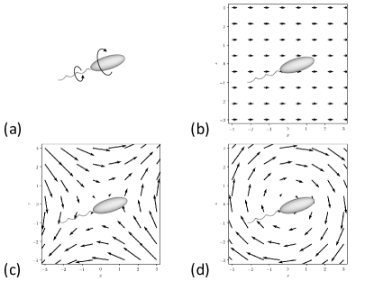
Figure 5: Sketch of the kinetic decoupling of the microswimmer in a external flow. (a) Active microswimmer motion $(\tilde{\bm{U}}_{a},\tilde{\bm{\Omega}}_{a})$ in bulk fluid at rest. (b) Passive microswimmer translation $\bm{u}_{b}$ in the external flow. (c) Passive microswimmer motion $(\tilde{\bm{U}}^{E},\tilde{\bm{\Omega}}^{E})$ in the symmetric (deviatoric) part of the external flow. (d) Passive microswimmer rotation $\bm{\Omega}_{p}^{S}$ in the antisymmetric part of the external flow.

Active motion. For the active part, we first numerically calculated the unit-spin motion $(\tilde{\bm{U}}_{a},\tilde{\bm{\Omega}}_{a})$ of a microswimmer swimming with $\omega_{t}=1$ pointed toward the $\textbf{X}_{3}$ direction with $(\theta=0,\phi=0,\psi=0,\psi_{t}=0)$. Thanks to the rotational symmetry of the ellipsoidal head, the last 2 rotational DOFs can be reduced to single DOF $\psi^{\prime}=\psi+\psi_{t}$. Indeed, if we take a given conformation on the swimmer and we applied a rotation of the entire swimmer of an angle $\psi=\alpha$ and then a rotation of the tail with respect to the head of and angle $\psi_{t}=-\alpha$ the initial and the final conformations are the same. Therefore, we can easily transform the motion $(\bm{U}_{a},\bm{\Omega}_{a})$ of an active swimmer whose tail spins at a rate $\Omega_{t}$ from the body coordinate frame $\textbf{O}^{\prime}\textbf{e}_{1}\textbf{e}_{2}\textbf{e}_{3}$ to the global coordinate frame $\textbf{O}\textbf{X}_{1}\textbf{X}_{2}\textbf{X}_{3}$

$$\bm{U}_{a}(\bm{\theta}_{c},\psi_{t}) =\Omega_{t}\bm{R}(\bm{\theta}_{c},\psi_{t})\tilde{\bm{U}}_{a}\,,$$ (27)

$$\bm{\Omega}_{a}(\bm{\theta}_{c},\psi_{t}) =\Omega_{t}\bm{R}(\bm{\theta}_{c},\psi_{t})\tilde{\bm{\Omega}}_{a}\,,$$ (28)

where the rotation matrix $\bm{R}$ (that transforms the expression of a vector in the body reference frame into its expression in the global reference frame) is a function of $\theta$, $\phi$ and $\psi^{\prime}$

$$\bm{R} =\begin{bmatrix}\mathrm{C}\phi\mathrm{C}\psi^{\prime}\mathrm{C}\theta-\mathrm{S}\phi\mathrm{S}\psi^{\prime}&-\mathrm{C}\psi^{\prime}\mathrm{S}\phi-\mathrm{C}\phi\mathrm{C}\theta\mathrm{S}\psi^{\prime}&\mathrm{C}\phi\mathrm{S}\theta\\ \mathrm{C}\psi^{\prime}\mathrm{C}\theta\mathrm{S}\phi+\mathrm{C}\phi\mathrm{S}\psi^{\prime}&\mathrm{C}\phi\mathrm{C}\psi^{\prime}-\mathrm{C}\theta\mathrm{S}\phi\mathrm{S}\psi^{\prime}&\mathrm{S}\phi\mathrm{S}\theta\\ -\mathrm{C}\psi^{\prime}\mathrm{S}\theta&\mathrm{S}\psi^{\prime}\mathrm{S}\theta&\mathrm{C}\theta\end{bmatrix}\,,$$ (29)

where $\mathrm{S}\theta$ stands for $\sin{(\theta)}$ and $\mathrm{C}\theta$ stands for $\cos{(\theta)}$ and so on.

Passive motion. Now, we discuss the passive part $(\bm{U}_{p},\bm{\Omega}_{p})$ induced by the external flow $\bm{u}_{b}$. This is a quite classical problem that we briefly revise for completeness kim1991microhydrodynamics ; happel2012low . Taylor expansion allows to locally decompose the generic flow field $\bm{u}_{b}$ into three parts,

$$u_{i}^{b}(\bm{x}_{c}+\delta\bm{x}_{c}) =u_{i}^{b}(\bm{x}_{c})+E_{ij}(\bm{x}_{c})\delta x_{j}^{c}+S_{ij}(\bm{x}_{c})\delta x_{j}^{c}\,,$$ (30)

$$E_{ij}(\bm{x}_{c}) =\dfrac{1}{2}(u_{i,j}^{b}(\bm{x}_{c})+u_{j,i}^{b}(\bm{x}_{c}))\,,$$ (31)

$$S_{ij}(\bm{x}_{c}) =\dfrac{1}{2}(u_{i,j}^{b}(\bm{x}_{c})-u_{j,i}^{b}(\bm{x}_{c}))\,,$$ (32)

where $E_{ij}$ and $S_{ij}$ are the symmetric and asymmetric part of the velocity gradient $u_{i,j}=\partial u_{i}/\partial x_{j}$. The first term of the right hand side of (30) gives a pure rigid body translation $\bm{U}_{p}^{b}(\bm{x}_{c})$ of the microswimmer without rotation, see Fig. 5(b). Instead, the effect of the last term induced a pure rigid body rotation $\bm{\Omega}_{p}^{S}=\frac{1}{2}\nabla\times\bm{u}^{b}$ where the $\nabla\times\bm{u}^{b}$ is the bulk fluid vorticity, see Fig. 5 (d).

$k$	strain rate base $\tilde{E}_{ij}^{k}$	associated flow $\tilde{u}_{i}^{Ek}$
$1$	$\begin{bmatrix}1&0&0\\ 0&-1&0\\ 0&0&0\end{bmatrix}$	$(x_{1},-x_{2},0)$
$2$	$\begin{bmatrix}0&0&0\\ 0&-1&0\\ 0&0&1\end{bmatrix}$	$(0,-x_{2},x_{3})$
$3$	$\begin{bmatrix}0&1&0\\ 1&0&0\\ 0&0&0\end{bmatrix}$	$(x_{2},x_{1},0)$
$4$	$\begin{bmatrix}0&0&1\\ 0&0&0\\ 1&0&0\end{bmatrix}$	$(x_{3},0,x_{1})$
$5$	$\begin{bmatrix}0&0&0\\ 0&0&1\\ 0&1&0\end{bmatrix}$	$(0,x_{3},x_{2})$

Table 1: Base flow associated with the decomposition of the symmetric component of the velocity gradient, see (34)

The contribution of the symmetric part of the gradient to the motion, Fig. 5(c), however, is more complex. $E_{ij}$ has nine components, but since it is symmetric, i.e. $E_{ij}=E_{ji}$, and the fluid is incompressible, i.e. $\mathrm{tr}(E_{ij})=E_{ii}=0$, only five of them are independent. Our approach is firstly to express the strain rate $E_{ij}$ in the body reference frame

$$\tilde{E}_{ij} =R^{T}E_{ij}R\,,$$ (33)

where $R$ is the rotation matrix (29). Then, we decompose it in five basic modes due to the linearity of the Stokes equations happel2012low ; chwang1975hydromechanics .

$$\tilde{E}_{ij} =\sum_{k=1}^{5}\tilde{\beta}_{k}\tilde{E}_{ij}^{k}\,,$$ (34)

Indeed, any $\tilde{E}_{ij}^{k}$ can be expressed as

$$\tilde{E}_{ij}=\begin{bmatrix}\beta_{1}&\beta_{3}&\beta_{4}\\ \beta_{3}&-\beta_{1}-\beta_{2}&\beta_{5}\\ \beta_{4}&\beta_{5}&\beta_{2}\end{bmatrix}\,,$$ (35)

by using the $5$ components reported in Table 1. Given this decomposition, we numerically solve the swimming kinematics $(\tilde{\bm{U}}_{k}^{E},\tilde{\bm{\Omega}}_{k}^{E})$ of the passive microswimmer for the five components and sum them with proper weights $\tilde{\beta}_{k}$

$$\tilde{\bm{U}}_{p}^{E}(\bm{x},\bm{\theta}_{c},\psi_{t}) =\sum_{k=1}^{5}\tilde{\beta}_{k}(\bm{x},\bm{\theta}_{c},\psi_{t})\tilde{\bm{U}}_{k}^{E}\,,$$ (36)

$$\tilde{\bm{\Omega}}_{p}^{E}(\bm{x},\bm{\theta}_{c},\psi_{t}) =\sum_{k=1}^{5}\tilde{\beta}_{k}(\bm{x},\bm{\theta}_{c},\psi_{t})\tilde{\bm{\Omega}}_{k}^{E}\,.$$ (37)

Finally, we express $\tilde{\bm{U}}_{p}^{E}$ and $\tilde{\bm{\Omega}}_{p}^{E}$ in the global reference frame

$$\bm{U}_{p}^{E}(\bm{x},\bm{\theta}_{c},\psi_{t}) =\bm{R}(\bm{\theta}_{c},\psi_{t})\tilde{\bm{U}}_{k}^{E}(\bm{x},\bm{\theta}_{c},\psi_{t})\,,$$ (38)

$$\bm{\Omega}_{p}^{E}(\bm{x},\bm{\theta}_{c},\psi_{t}) =\bm{R}(\bm{\theta}_{c},\psi_{t})\tilde{\bm{\Omega}}_{k}^{E}(\bm{x},\bm{\theta}_{c},\psi_{t})\,.$$ (39)

It is worth noting that the weights $\tilde{\beta}_{k},k=1\dots 5$ are functions of external flow $\bm{u}_{b}$ and swimmer configuration $(\bm{\theta}_{c},\psi_{t})$ and they do not vary with the geometric details of the microswimmer. Similar strategies for calculating the passive motion of the microswimmer can be found in marath2018inertial ; subramanian2006inertial .

In summary, the microswimmer generalized velocity in an external flow is obtained as

$$\bm{U} =\Omega_{t}\bm{R}\tilde{\bm{U}}_{a}+\bm{U}_{p}^{b}+\bm{R}\sum_{k=1}^{5}\tilde{\beta}_{k}\tilde{\bm{U}}_{k}^{E}\,,$$ (40)

$$\bm{\Omega} =\Omega_{t}\bm{R}\tilde{\bm{\Omega}}_{a}+\bm{\Omega}_{p}^{S}+\bm{R}\sum_{k=1}^{5}\tilde{\beta}_{k}\tilde{\bm{\Omega}}_{k}^{E}\,.$$ (41)

A sketch of the proposed decoupling is reported in Fig. 5. The main advantage of this method is that, for given geometry of microswimmer, regardless the tail spin rate $\Omega_{t}$, only six simulations are necessary; one for getting $(\tilde{\bm{U}}_{a},\tilde{\bm{\Omega}}_{a})$ and five for $(\tilde{\bm{u}}_{k}^{E},\tilde{\bm{\Omega}}_{k}^{E}),k=1\dots 5$. Thus, one can obtain these quantities accurately previously, and then solve the microswimmer kinematics (22)-(24).

For the microswimmer motion in the shear flow $\bm{u}_{b}=(X_{3},0,0)$, we have

$$E_{ij} =\dfrac{1}{2}\begin{bmatrix}0&0&1\\ 0&0&0\\ 1&0&0\end{bmatrix}\,,$$ (42)

that, using (33) and (34), gives

$$\tilde{\beta}_{1} =\mathrm{C}\psi^{\prime}(\mathrm{S}\phi\mathrm{S}\psi^{\prime}-\mathrm{C}\phi\mathrm{C}\psi^{\prime}\mathrm{C}\theta)\mathrm{S}\theta\,,$$ (43)

$$\tilde{\beta}_{2} =\mathrm{C}\phi\mathrm{C}\theta\mathrm{S}\theta\,,$$ (44)

$$\tilde{\beta}_{3} =\dfrac{1}{4}(2\mathrm{C}(2\psi^{\prime})\mathrm{S}\phi\mathrm{S}\theta+\mathrm{C}\phi\mathrm{S}(2\psi^{\prime})\mathrm{S}(2\theta))\,,$$ (45)

$$\tilde{\beta}_{4} =\dfrac{1}{2}(\mathrm{C}\phi\mathrm{C}\psi^{\prime}\mathrm{C}(2\theta)-\mathrm{C}\theta\mathrm{S}\phi\mathrm{S}\psi^{\prime})\,,$$ (46)

$$\tilde{\beta}_{5} =\dfrac{1}{2}(-\mathrm{C}\psi^{\prime}\mathrm{C}\theta\mathrm{S}\phi-\mathrm{C}\phi\mathrm{C}(2\theta)\mathrm{S}\psi^{\prime})\,.$$ (47)

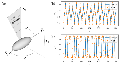
Figure 6: Validation of the numerical method: Jeffery orbits. (a) Sketch of an ellipse orbit in a shear flow. The shear flow is in the $\textbf{X}_{1}\textbf{X}_{3}$ plane of the global coordinate frame $\textbf{O}\textbf{X}_{1}\textbf{X}_{2}\textbf{X}_{3}$. The polar $\theta$ and azimuthal $\phi$ angles are used to describe the orientation of the body frame with respect to the global frame. The unit vector $\bm{p}$ denotes the orientation of the ellipsoid. (b, c) Time evolution of angles $\theta$ and $\phi$ for an ellipse with aspect ratio $r_{h1}/r_{h2}=3$ moving in a shear flow. The initial orientation of the ellipse is $(\theta=0.21\pi,\phi=0.23\pi)$. Orange points represent our numerical solution while the analytical solution kim1991microhydrodynamics are reported as blue lines.

To test our approach, we reproduced the Jeffery orbit jeffery1922motion for a $r_{h1}/r_{h2}=3$ ellipse in a shear flow, see fig 6.

References

- [1] Howard C Berg. E. coli in Motion. Springer Science & Business Media, 2008.
- [2] Chen Qian, Chui Ching Wong, Sanjay Swarup, and Keng-Hwee Chiam. Bacterial tethering analysis reveals a “run-reverse-turn” mechanism for pseudomonas species motility. Applied and environmental microbiology, 79(15):4734–4743, 2013.
- [3] Paolo Sartori, Enrico Chiarello, Gaurav Jayaswal, Matteo Pierno, Giampaolo Mistura, Paola Brun, Adriano Tiribocchi, and Enzo Orlandini. Wall accumulation of bacteria with different motility patterns. Physical Review E, 97(2):022610, 2018.
- [4] Li Zhang, Kathrin E Peyer, and Bradley J Nelson. Artificial bacterial flagella for micromanipulation. Lab on a Chip, 10(17):2203–2215, 2010.
- [5] Rami Mhanna, Famin Qiu, Li Zhang, Yun Ding, Kaori Sugihara, Marcy Zenobi-Wong, and Bradley J Nelson. Artificial bacterial flagella for remote-controlled targeted single-cell drug delivery. Small, 10(10):1953–1957, 2014.
- [6] Eric Lauga and Thomas R Powers. The hydrodynamics of swimming microorganisms. Reports on Progress in Physics, 72(9):096601, 2009.
- [7] Jens Elgeti, Roland G Winkler, and Gerhard Gompper. Physics of microswimmers—single particle motion and collective behavior: a review. Reports on progress in physics, 78(5):056601, 2015.
- [8] Eric Lauga, Willow R DiLuzio, George M Whitesides, and Howard A Stone. Swimming in circles: motion of bacteria near solid boundaries. Biophysical journal, 90(2):400–412, 2006.
- [9] Giorgia Guccione, Daniela Pimponi, Paolo Gualtieri, and Mauro Chinappi. Diffusivity of e. coli-like microswimmers in confined geometries: The role of the tumbling rate. Physical Review E, 96(4):042603, 2017.
- [10] H Shum, EA Gaffney, and DJ Smith. Modelling bacterial behaviour close to a no-slip plane boundary: the influence of bacterial geometry. Proceedings of the Royal Society A: Mathematical, Physical and Engineering Sciences, 466(2118):1725–1748, 2010.
- [11] R Di Leonardo, D Dell’Arciprete, L Angelani, and V Iebba. Swimming with an image. Physical review letters, 106(3):038101, 2011.
- [12] Daniela Pimponi, Mauro Chinappi, Paolo Gualtieri, and Carlo Massimo Casciola. Hydrodynamics of flagellated microswimmers near free-slip interfaces. Journal of Fluid Mechanics, 789:514–533, 2016.
- [13] Jinglei Hu, Adam Wysocki, Roland G Winkler, and Gerhard Gompper. Physical sensing of surface properties by microswimmers–directing bacterial motion via wall slip. Scientific reports, 5:9586, 2015.
- [14] Silvio Bianchi, Filippo Saglimbeni, Giacomo Frangipane, Dario Dell’Arciprete, and Roberto Di Leonardo. 3d dynamics of bacteria wall entrapment at a water–air interface. Soft matter, 15(16):3397–3406, 2019.
- [15] Henry C Fu, Thomas R Powers, and Roman Stocker. Bacterial rheotaxis. Proceedings of the National Academy of Sciences, 109(13):4780–4785, 2012.
- [16] Marcos, Henry C. Fu, Thomas R. Powers, and Roman Stocker. Separation of microscale chiral objects by shear flow. Phys. Rev. Lett., 102:158103, Apr 2009.
- [17] Roberto Rusconi, Jeffrey S Guasto, and Roman Stocker. Bacterial transport suppressed by fluid shear. Nature physics, 10(3):212, 2014.
- [18] Philipp Kanehl and Takuji Ishikawa. Fluid mechanics of swimming bacteria with multiple flagella. Physical Review E, 89(4):042704, 2014.
- [19] Emily E Riley, Debasish Das, and Eric Lauga. Swimming of peritrichous bacteria is enabled by an elastohydrodynamic instability. Scientific reports, 8, 2018.
- [20] J Einarsson, BM Mihiretie, A Laas, S Ankardal, JR Angilella, D Hanstorp, and B Mehlig. Tumbling of asymmetric microrods in a microchannel flow. Physics of Fluids, 28(1):013302, 2016.
- [21] Jonas Einarsson. Angular dynamics of small particles in fluids. PhD thesis, Department of Physics, University of Gothenburg, 2015.
- [22] Ian Thorp and John Lister. Motion of a non-axisymmetric particle in viscous shear flow. Journal of Fluid Mechanics, 2019.
- [23] Howard C Berg and Linda Turner. Torque generated by the flagellar motor of escherichia coli. Biophysical journal, 65(5):2201–2216, 1993.
- [24] Jianhua Xing, Fan Bai, Richard Berry, and George Oster. Torque–speed relationship of the bacterial flagellar motor. Proceedings of the National Academy of Sciences, 103(5):1260–1265, 2006.
- [25] DL Young, SJ Jane, CM Fan, K Murugesan, and CC Tsai. The method of fundamental solutions for 2d and 3d stokes problems. Journal of Computational Physics, 211(1):1–8, 2006.
- [26] See Supplemental Material at [URL will be inserted by publisher] for movies showing these trajectories.
- [27] See Supplemental Material at [URL will be inserted by publisher] for a figure representing the dependence of the final stable trajectory on initial swimmer orientation.
- [28] Howard Berg. Motile behavior of bacteria. Physics today, 2000.
- [29] Bin Liu, Kenneth S Breuer, and Thomas R Powers. Propulsion by a helical flagellum in a capillary tube. Physics of Fluids, 26(1):011701, 2014.
- [30] C Rorai, M Zaitsev, and S Karabasov. On the limitations of some popular numerical models of flagellated microswimmers: importance of long-range forces and flagellum waveform. Royal Society open science, 6(1):180745, 2019.
- [31] Ricardo Cortez, Lisa Fauci, and Alexei Medovikov. The method of regularized stokeslets in three dimensions: analysis, validation, and application to helical swimming. Physics of Fluids, 17(3):031504, 2005.
- [32] Bokai Zhang, Yang Ding, and Xinliang Xu. Active suspensions of bacteria and passive objects: a model for the near field pair dynamics. arXiv preprint arXiv:2002.04693, 2020.
- [33] Evert Klaseboer, Qiang Sun, and Derek YC Chan. Non-singular boundary integral methods for fluid mechanics applications. Journal of Fluid Mechanics, 696:468–478, 2012.
- [34] GP Muldowney and Jonathan JL Higdon. A spectral boundary element approach to three-dimensional stokes flow. Journal of Fluid Mechanics, 298:167–192, 1995.
- [35] Arnold JTM Mathijssen, Nuris Figueroa-Morales, Gaspard Junot, Éric Clément, Anke Lindner, and Andreas Zöttl. Oscillatory surface rheotaxis of swimming e. coli bacteria. Nature communications, 10(1):1–12, 2019.
- [36] Sangtae Kim and Seppo J Karrila. Microhydrodynamics: principles and selected applications. Courier Corporation, 1991.
- [37] Ali Najafi and Ramin Golestanian. Simple swimmer at low reynolds number: Three linked spheres. Physical Review E, 69(6):062901, 2004.
- [38] Abdallah Daddi-Moussa-Ider, Maciej Lisicki, and Arnold JTM Mathijssen. Tuning the upstream swimming of microrobots by shape and cargo size. Physical Review Applied, 14(2):024071, 2020.
- [39] Yasser Aboelkassem and Anne E Staples. Stokeslets-meshfree computations and theory for flow in a collapsible microchannel. Theoretical and Computational Fluid Dynamics, 27(5):681–700, 2013.
- [40] Duncan A Lockerby and B Collyer. Fundamental solutions to moment equations for the simulation of microscale gas flows. Journal of Fluid Mechanics, 806:413–436, 2016.
- [41] Considering one-quarter of an ellipse, the arc length is a monotone increasing function of the eccentric angle that has no explicit expression. Therefore, we first fit this function using a quadratic polynomial, then determine a set of that keeps the distance between two adjacent points approximately equal. Finally we calculate the location of the points on the plane, see [42].
- [42] Andy Jones. How to divide an ellipse to equal segments? https://stackoverflow.com/questions/20197974/how-to-divide-an-ellipse-to-equal-segments, 2013. [Online; accessed 6-August-2020].
- [43] Youcef Saad and Martin H Schultz. Gmres: A generalized minimal residual algorithm for solving nonsymmetric linear systems. SIAM Journal on scientific and statistical computing, 7(3):856–869, 1986.
- [44] Satish Balay, William D Gropp, Lois Curfman McInnes, and Barry F Smith. Efficient management of parallelism in object-oriented numerical software libraries. In Modern software tools for scientific computing, pages 163–202. Springer, 1997.
- [45] Satish Balay, Shrirang Abhyankar, Mark F. Adams, Jed Brown, Peter Brune, Kris Buschelman, Lisandro Dalcin, Alp Dener, Victor Eijkhout, William D. Gropp, Dmitry Karpeyev, Dinesh Kaushik, Matthew G. Knepley, Dave A. May, Lois Curfman McInnes, Richard Tran Mills, Todd Munson, Karl Rupp, Patrick Sanan, Barry F. Smith, Stefano Zampini, Hong Zhang, and Hong Zhang. PETSc Web page. https://www.mcs.anl.gov/petsc, 2019.
- [46] Daniela Pimponi, Mauro Chinappi, and Paolo Gualtieri. Flagellated microswimmers: Hydrodynamics in thin liquid films. The European Physical Journal E, 41(2):1–8, 2018.
- [47] Basile Graf. Quaternions and dynamics. arXiv preprint arXiv:0811.2889, 2008.
- [48] James Diebel. Representing attitude: Euler angles, unit quaternions, and rotation vectors. Matrix, 58(15-16):1–35, 2006.
- [49] P Bogacki and Lawrence F Shampine. An efficient runge-kutta (4, 5) pair. Computers & Mathematics with Applications, 32(6):15–28, 1996.
- [50] Shrirang Abhyankar, Jed Brown, Emil M Constantinescu, Debojyoti Ghosh, Barry F Smith, and Hong Zhang. Petsc/ts: A modern scalable ode/dae solver library. arXiv preprint arXiv:1806.01437, 2018.
- [51] John Happel and Howard Brenner. Low Reynolds number hydrodynamics: with special applications to particulate media, volume 1. Springer Science & Business Media, 2012.
- [52] Allen T Chwang and T Wu. Hydromechanics of low-reynolds-number flow. part 2. singularity method for stokes flows. Journal of Fluid mechanics, 67(4):787–815, 1975.
- [53] G Subramanian and DL Koch. Inertial effects on the orientation of nearly spherical particles in simple shear flow. Journal of Fluid Mechanics, 557:257, 2006.
- [54] Mahan Raj Banerjee and Ganesh Subramanian. An anisotropic particle in a simple shear flow: an instance of chaotic scattering. arXiv preprint arXiv:2005.11157, 2020.
- [55] Navaneeth K Marath and Ganesh Subramanian. The inertial orientation dynamics of anisotropic particles in planar linear flows. Journal of Fluid Mechanics, 844:357, 2018.
- [56] George Barker Jeffery. The motion of ellipsoidal particles immersed in a viscous fluid. Proceedings of the Royal Society of London. Series A, Containing papers of a mathematical and physical character, 102(715):161–179, 1922.