Collective transport via sequential caging

Abstract

We propose a decentralized algorithm to collaboratively transport arbitrarily shaped objects using a swarm of robots. Our approach starts with a task allocation phase that sequentially distributes locations around the object to be transported starting from a seed robot that makes first contact with the object. Our approach does not require previous knowledge of the shape of the object to ensure caging. To push the object to a goal location, we estimate the robots required to apply force on the object based on the angular difference between the target and the object. During transport, the robots follow a sequence of intermediate goal locations specifying the required pose of the object at that location. We evaluate our approach in a physics-based simulator with up to 100 robots, using three generic paths. Experiments using a group of KheperaIV robots demonstrate the effectiveness of our approach in a real setting.

1 Introduction

Several insect species exhibit an incredible level of coordination to lift and carry heavy objects to their nest, whether for building materials or food. Paratrechina longicornis can collectively transport heavy food from a source location to its nest purely through local interaction with neighboring ants [10]. These ants are capable of carrying an object of arbitrary shape and ten times heavier than their bodies by collaborating in an effective manner. Designing approaches to realize collaborative transport using a group of robots can find its application in warehouse management [19] and collaborative construction of structures [14].

Figure 1: Illustration of the process of object transpiration, with the robots starting from a deployment cluster, caging the object and transporting the object.

In this work, we take inspiration from these natural insect species to design an approach to collaboratively transport heavy objects (i.e. that cannot be carried by a single robot) of arbitrary shape using a swarm of robots. The main challenges of this type of collective transport are: 1. the effective placement of robots around the transported object, 2. the effective application of force around the object to avoid tugs-of-war, and 3. adapting to the objects center-of-mass movement and the alignment of forces between neighbors. Our approach starts with a task allocation phase, where the robots are sequentially deployed around the object, a process known as caging [23]. Completing the task allocation phase, the robots transport the object towards a target location as shown in fig. 1.

Collaborative transport is a well-studied topic: some approaches use ground robots [14, 24, 7, 3] for cooperative manipulation either with explicit communication [8] or force based coordination [9], while others use quadcopters carrying a cable-suspended [5] or rigidly attached [27] object that is heavier than one robot’s maximum payload.

Many of the approaches discussed earlier do not explicitly consider robot’s interaction with other robots to continuously maintain cage formation, while including an obstacle avoidance mechanism within their control framework. This latter is particularly limiting when the perimeter of the pushed object is small, as it might prevent the robots to get close to the object to apply an effective force. In our approach, we design a sequential placement of robots to avoid this scenario and maintain the initial formation continuously while moving.

Approaches like [2] assume that the position and shape of the object is either continuously known or periodically updated using a central system. Measuring the position and shape of the object in a real world scenarios might be difficult and would limit the use of the transport system to some indoor applications. Furthermore, some approaches either assume that the robots are readily placed around the object to be manipulated [20] and design control strategies for the manipulation of the object. A few approaches provide emphasis on caging or design a control policy for a specific type of caging [13]. In this paper, we design a complete system that allows the robots to start from a deployment cluster and take up positions around the object to be transported, in a way that is similar to [7]. Our approach periodically estimates the centroid of the object using only the relative positional information shared by neighboring robots, avoiding the need to have continuous external measurements. Our task allocation allows heterogeneous robots with varying capabilities (e.g. path planning), as well as provides a way to addressing robot failures [22]. We provide sufficient conditions for the convergence of our caging, and show that our approach terminates for convex objects.

2 Related Work

The concept of caging was first introduced by Rimon and Blake [18] for a finger gripper. Caging is a concept of trapping the object to be manipulated by a gripping actuator, in our work we use a group of robots to act as a single entity to grip the object using form closure as in [23]. A simple form of caging and leader-follower based strategies [26] are employed to push the object by sensing the resultant forces. The main constraint of these works is that the robots cannot follow paths with sharp turns.

Pereira et al. [13] introduce a new type of caging called object closure, in which the object to be transported is loosely caged until the configuration satisfies certain conditions in an imaginary closure configuration space. Each robot in the team has to estimate the orientation and position of the object to use this approach. Wan et al. [23] propose robust caging to minimize the number of robots to form closure using translation and rotation constraints. Wan et al. also extended their work for polygons, balls and cylinders to be transported on a slope [24]. This approach requires continuous positional updates from an external system and uses a central system to compute the minimum number of robots required.

An approach to caging L-shaped objects is proposed in [7]: the robots switch between different behavioral states to approach the object and achieve potential caging. This approach requires the robots to know certain properties of the object beforehand, such as the minimum and maximum diameter of the caged object. A caging strategy for polygonal convex objects is proposed in [6], the approach uses a sliding mode fuzzy controller to traverse predefined paths. A leader robot coordinates the transportation using the relative position of all the other robots.

Gerkey et. al. [11] propose a strategy for pushing an object by assigning “pushers” and “watchers”. Watchers monitor the position of the object and other robots, while pushers perform the pushing task. The approach provides fault tolerance to robot failures and relies heavily on the performance of the watchers. Chen et al. [3] propose an approach in which the robots are placed around an object that occludes the transportation destination: the robots that do not see the destination are the ones that push the object. The intuition behind this placement is that the location that is most effective for pushing the object is the occluded region, i.e. the opposite side of the direction of movement. Our strategy is similar to [3], where we estimate the angular difference between the object and the goal using the proximity sensor, and only the robots that are below a threshold apply a force to the object. Our approach places robots all around the object to adjust and follow a sequence of changing target location, as opposed to only placing robots in the occluded region [3].

The work in [25] combines reinforcement learning and evolutionary algorithms to coordinate 3 types of agents to learn to push an object. “Vision robots” estimate the positions of the object and other robots, “evolutionary learning agents” generate plans for the “worker robots”, and these latter execute the plan to push the object. Alkilabi et al. [1] use an evolutionary algorithm to tune a recurrent neural network controller that allows a group of e-puck robots to collaboratively transport a heavy object. The robots use an optical flow sensor to determine and achieve an alignment of forces. The authors demonstrate that the approach works well for different object sizes and shapes, however, the proper functioning of the algorithm relies heavily on the performance of the optical flow sensors.

3 Methodology

Fig. LABEL:fig:State_machine shows the high level state machine used in our collaborative transport behavior. At initialization, the robots enter into a sequence of task allocation rounds allowing the robots to take up positions around the object to be transported with a desired inter-robot distance. Once caging is complete, the robots that are a part of the object cage agree on the desired object path and start pushing and rotating the object. The path is represented as a sequence of points, and all the robots in the cage use a barrier (i.e. they wait for consensus) to go through each intermediate point.

3.1 Problem Formulation

Let $C_{o}(t)\in\mathbb{R}^{2}$ be the centroid of an arbitrary shaped object at time $t$, $x_{i}(t)\in\mathbb{R}^{2}$ the position of robot $i$ at time $t$, and $X(t)=\{x_{1}(t),x_{2}(t),...,x_{n}(t)\}$ the set containing the positions of the robots at time $t$. Let $S_{o}$ be a closed, convex set representing the perimeter of the object to be transported. Given a sequence of target locations $\mathbb{T}=\{\tau_{1},\tau_{2},...,\tau_{n}\}$ the task of the robots is to take up locations around the perimeter of the object $S_{o}$ with a desired inter-robot distance $I_{d}\in\mathbb{R}$ and drive the centroid of the object $C_{o}$ from a known initial state $C_{o}(0)$ to a final state $C_{o}(t_{f})$ at some time $t_{f}$, passing through the target locations in $\mathbb{T}$.

We assume that the robots can perceive the goal in the environment and know an estimate of the initial centroid location $C_{o}(0)$ of the object to be transported. The mass of the object is assumed to be proportional to the size with a minimum density for the object. We also assume that the line connecting two subsequent targets $\tau_{x-1}$ and $\tau_{x}$ does not go through obstacles and the perimeter of the object $S_{o}$ to be transported is greater than $3*I_{d}$. We consider a point mass model for the robots ($\dot{x}_{i}(t)=u_{i}$) and assume that the robots are fully controllable with $u_{i}$. The robots are assumed to be equipped with a range and bearing sensor to determine the relative positional information and communicate with neighboring robots within a small fixed communication range $d_{C}$. In our experiments, we used KheperaIV robots that are equipped with 8 proximity sensors at equal angles around the robot, and we assume similar capabilities in general.

Figure 3: Illustration of the process of task allocation based caging (a) illustrate the process of edge following to reach the new target (b) the stopping condition to terminate caging.

3.2 Task Allocation based Caging

Consider a group of robots randomly distributed in a cluster and a known initial position of the object. The goal of the robots is to deploy to suitable location around the perimeter of the object $C_{o}$ to guarantee object closure while respecting the required inter-robot distance $I_{d}$.

The caging process starts with the allocation of the first task (an estimation of the centroid of the object) to a seed robot (closest robot to the object, elected via bidding) as shown in Figure 3 (a). The seed robot moves towards the center of the object until it detects the object with its on-board proximity sensors. As the seed robot touches the object, it creates two target locations (one to its left and one to its right, called branches). The robots bid for these new target locations and continue the process of spawning the new targets along their branch until the minimum distance between robots in the two branches is smaller than $d_{T}$.

Our task allocation algorithm performs the role of determining the appropriate target around the object for each robot, the caging targets. We consider a Single Allocation (SA) problem [4], where every robot is assigned a single task. The caging targets are sequentially available to the robots, i.e. a new target becomes available after a robot has reached its target. Note that these targets are considered to be approximate (created by establishing a local coordinate system like in [21]), hence they are refined by the robots using their proximity sensors and the position of the closest robot in the branch on reaching the assigned target. The approach of sequential caging is particularly appropriate for scenarios where the shape of the object is initially or continuously unknown, the robots sequentially assign robots to the closure and enclose the transported object.

We use a bidding algorithm [22] (described in the supplementary material ): the robots locally compute bids for a task and recover the lowest bid of the team from a distributed, shared tuple space [16]. The robots update the tuple space if the local bid is lower, with conflicts resolved using the procedure outlined in [22]). After a predetermined allocation time ($T_{a}$), the lowest bid in the tuple space is declared as the winner. $T_{a}$ has to be selected considering the communication topology and delays to avoid premature allocation as detailed in [22].

To reach the assigned target, the robots edge-follow the neighbors in their target branch. The control inputs ($u_{i}$) are generated using range and bearing information from neighbors: the robots find their closest neighbor and create a neighbor vector $x_{n}$ using the range and bearing information. The control inputs are then $u_{i}=(\perp x_{n})+(||x_{n}||-I_{d})*x_{n}$; the first term makes sure the robot orbits the neighbor and the second term applies a pulling or pushing force to keep the robot at distance $I_{d}$. On reaching the target (detected using the proximity sensors), the robot measure the distance to the closest neighbor of the branch and apply a distance correction to keep the inter-robot caging distance to be $I_{d}$. The robot creates an obstacle vector using the proximity values: $x_{o}=\frac{\sum_{i\in P}p_{i}}{|P|}$, with $P=\{p_{0},..,p_{7}\},p_{i}\in\mathbb{R}^{2}$ being the set containing the individual proximity readings as vectors. The inter-robot distance correction control inputs are generated using: $u_{i}=\perp x_{o}$. When there are not enough robots to complete the caging, the robots can adapt by increasing $I_{d}$ and applying inter-robot distance correction control until the termination condition is met.

Proposition 1 Consider two sets L and R denoting the left and right branch respectively, L contains all the attachment points of the left branch robots to the object, and R contains the attachment points on the right branch. The caging terminates if $\exists p\in L,q\in R$ such that $d_{pq}\leq d_{T}$ while $d_{lr}>d_{T}\quad\forall l\in L-\{p\}\wedge\forall r\in R-\{q\}$.

Referring to fig. 3(b), consider two closed, convex sets, $L_{o}=\{l_{1},...,l_{n}\}$ containing all the points on the curve $l_{1}l_{n}$ and $R_{o}=\{r_{1},...,r_{n}\}$ containing all the points on the curve $r_{1}r_{n}$. Set $L_{o}$ and $R_{o}$ are ordered and the distance between the two constitutive points satisfy $d(l_{n},l{n-1})>d_{T}$.

3.3 Behaviors for pushing and rotating

Once two robots around the perimeter of the object satisfy the termination condition and a consensus is reached on the path, the robots initiate the target following routine. The path is represented as a sequence of desired object centroid target locations $\mathbb{T}$ and each entry $\tau_{i}=(\tau_{p},\tau_{r})$, with $\tau_{p}\in\mathbb{R}^{2}$ and $\tau_{r}\in[0,2\pi]$. $\tau_{p}$ is the local target location and $\tau_{r}$ is the desired object orientation along the z-axis (yaw) at that target location. The main intuition behind having these local targets is to use a geometric path planner. One of the robot in the swarm with the ability to compute a path to the user defined target $\tau_{n}$ compute the path and share it as a sequence of states(targets) using virtual stigmergy [16]. The robots sequentially traverse the targets in $\mathbb{T}$, on reaching a $\tau_{p}$, the robots rotate the object to $\tau_{r}$. Each robot in caging computes $u_{fp}$ as in equ. 1 to exert a forward force and push the object. Similarly, for rotating the object the robots apply $u_{fr}$ as in equ. 2.

$$u_{fp} =u_{t}+u_{f}+u_{cp},$$ (1)

$$u_{fr} =u_{r}+u_{f}+u_{cr}$$ (2)

where, $u_{t}$ and $u_{r}$ are a force to move the object towards the target by pushing, and a torque to rotate the object to the desired angle, respectively. $u_{f}$, as shown in equ. 3, is the contribution that makes sure the robots stay in the same formation. $u_{cp}$ (equ. 4) and $u_{cr}$ (equ. 5) are contributions that ensure the robots stay in contact with the object during pushing and rotation.

Maintaining Formation The robot formation from the caging operation tends to get distorted as a result of its application of pushing force on the object to move it towards the target. The robots in the cage apply a force to stay in this formation throughout the transportation task: they store a set $\textit{N}_{f}=\{(d_{i},\theta_{i})|d_{i}\leq k*I_{d},\forall i\in\textit{N}\}$ that contains the range and bearing measurements of their neighbors, with $k$ being a design parameter. The control input $u_{f}$ to maintain formation is:

$$u_{f}=\sum_{\forall i\in\textit{N}_{f}}{\frac{K_{f}(d_{i}-d_{cur})}{d_{i}}}\begin{bmatrix}d_{i}\cos{\theta_{i}}-\cos{\frac{\theta_{i}-\theta_{cur}}{\theta_{i}}}\\ d_{i}\sin{\theta_{i}}-\sin{\frac{\theta_{i}-\theta_{cur}}{\theta_{i}}}\end{bmatrix}$$ (3)

The first term in the equ. 3 is the desired inter-agent distance correction, while the second term applies the desired orientation correction. This formulation is inspired from the commonly used edge potential to preserve a lattice structure among the robots [12]. We apply this edge potential among adjacent robots in a cage to preserve the formation and the desired inter-agent distance.

Maintaining contact with the Object The robots in the formation need to determine if they need to apply a force and stay in contact with the object. During pushing, the robots apply a control input to stay in contact with the object, determining its effectiveness in pushing as in equ. 4. The effectiveness of a robot’s pushing depends on the position of the robot with respect to the object and the target.

The angle $\theta_{p}$ (a parameter) determines if the robot is an effective pusher: if the angle between the object $x_{o}$ and the target $\tau_{p}$ is greater or equal to $\theta_{p}$, pushing is considered effective, and the robots apply an input $u_{cp}$ to maintain contact. Similarly, the robots apply $u_{cr}$ to maintain contact during rotations:

$$u_{cp} =\begin{cases}[0,0]^{T},&\angle(x_{o},\tau_{p})\geq\theta_{p}\\ \frac{K_{cp}x_{o}}{||x_{o}||},&\angle(x_{o},\tau_{p})<\theta_{p}\end{cases}$$ (4)

$$u_{cr} =\frac{K_{cr}x_{o}}{||x_{o}||}$$ (5)

where $x_{o}$ is the proximity vector that determines the current object location in robots coordinate system, and $\theta_{p}$, $K_{cp}$ and $K_{cr}$ are design parameters. $\theta_{p}$ is a design parameter that defines the effective pushing perimeter around the object, as shown in fig. 4.

Applying forces The robots have to exert force in the right direction to move and rotate the object according to the targets in $\mathbb{T}$. The robots must apply force in the desired angular window around the perimeter of the object to avoid tugs-of-war. The control inputs $u_{t}$ and $u_{r}$ make sure the robots exert the force in the right direction:

$$u_{t} =\begin{cases}[0,0]^{T},&||\tau_{p_{l}}-x_{i}||\leq d_{tol}\\ \frac{K_{t}[\tau_{p_{l}}-x_{i}]}{||\tau_{p_{l}}-x_{i}||},&||\tau_{p_{l}}-x_{i}||>d_{tol}\end{cases}$$ (6)

$$u_{r} =\begin{cases}\begin{bmatrix}0&-1\\ 1&0\end{bmatrix}\frac{K_{r}(x_{i}-C_{o})}{||x_{i}-C_{o}||},&\angle(\tau_{p},C_{o})<\theta_{r}\\ [0,0]^{T},&\angle(\tau_{p},C_{o})\geq\theta_{r}\end{cases}$$ (7)

where, $d_{tol}$ is a design parameter that defines the distance tolerance, $\tau_{p_{l}}$ is the local target computed by the robot using the centroid position and its position along the perimeter of the object. On reaching an intermediate target $\tau_{i}$ the robots share their approximate position with respect to a common coordinate system computed as in [21] in a distributed, shared tuple space [16] with all the other robots. The robots retrieve this positional information and compute the centroid of the object $C_{o}$, which is then used during the rotation of the object.

Figure 4: Illustration of the resultant force and the angle of effective robots, the effective pushing positions on the perimeter of the object is shown in green.

As in [3], we can prove that the object reaches the goal as $t\to\infty$, with the difference being that the robots exerting force are not based on the occluded perimeter of the object, but are instead the robots satisfying $\angle(x_{o},\tau_{p})<\theta_{p}$.

Theorem 3.1.

The distance between the centroid of the object $C_{o}$ and the target location $\tau_{p}$ strictly decreases if the velocity of the transported object is governed by the translation dynamics equation of the object $\dot{v_{o}}=kF$. For $t\to\infty$, the center of the object $C_{o}$ reaches $\tau_{p}$, where $\dot{v_{o}}$ is the derivative of the object velocity and $kF$ is the fraction of the force that is transfered to the object from the robots.

Proof 3.2.

Fig. 4 shows the resultant F transferred from the robots to the object and the effective angular window (along the curve cTd) on the perimeter of the object to exert force. Consider all the robots along the curve cTd are applying a force using a control input determined by the unit vector $u_{t}$. The overall force transferred to the object is $F=(c_{x}-c_{y})-(d_{x}-d_{y})$, which is the tangent vector $(d-c)$ rotated by ($\frac{\pi}{2}$) [3].

Consider the squared distance between the target $\tau_{p}=[0,0]^{T}$ and centroid $C_{o}$ at time t to be $d_{g}(t)=||\tau_{p}-C_{o}||^{2}$, taking the time derivative gives $\dot{d_{g}}=2k*C_{o}*F$, substituting F with the resultant force gives $\dot{d_{g}}=k*((C_{o_{y}}c_{x}-C_{o_{x}}c_{y})-(C_{o_{y}}d_{x}-C_{o_{x}}d_{y}))$. The distance $d_{g}(t)\geq 0,\forall t>0$, when the center of the object lies outside the desired goal $\tau_{p}$ and since $C_{o}*F<0$ is strictly decreasing because of the force applied by the robots, we get $\lim_{t\to\infty}\dot{d_{g}}=0$. In other words, the center $C_{o}$ will eventually reach the goal $\tau_{p}$.

4 Experiments

We performed a set of experiments in a physics-based simulator (ARGoS3 [17]) with a KheperaIV robot model under various conditions to study the performance of our approach. We implemented our behavioral state machine for the robots using Buzz [15]. We set the number of robots $N_{r}\in\{25,50,100\}$ and adapt the size $S\in\{[2,2],[3.6,6],[7.2,12]\}m$ and mass $M\in\{5.56,30.024,120.096\}kg$ of a cuboid object according to the number of robots. The mass of the object is calculated assuming a constant density hollow material. In another set of experiments, we used three irregular objects: cloud, box rotation, and clover. We set the design parameters of the algorithm to the values shown in Tab. 1. We choose the gain parameters for maintaining formation($k_{f}$), contact with object($k_{cp}$) and force application ($k_{t}$) based on several rounds of trail-and-error simulations. The tolerance parameters $d_{tol}$ and Orient. tol. are chosen to fit our non-holonomic robots: a large part of the error shown in fig. 7 is due to the non-holonomic nature of our robots. We evaluate the various performance metrics over three benchmark paths: a straight line, a zigzag, and straight line with two $90\mathrm{°}$ rotations (straight_rot in Fig. 5). All the paths consists of 9 waypoints (WPs) and straight_rot has its rotations at WP 3 and 6. Each experiment is repeated 30 times with random initial conditions.

Table 1: Experimental parameters

Caging $d_{s}$ 0.35m $I_{d}$ 0.45m $d_{tol}$ 0.05m $d_{T}$ $1.85I_{d}$ $K_{t}$ 30 Prox. thres. 0.7

Pushing $\theta_{p}$ $115^{\circ}$ $K_{cp}$ 40($<115^{\circ}$), 20($\geq 115^{\circ}$) $d_{tol}$ 0.1m $K_{f}$ 40 $K_{t}$ 60 Barrier 90%

Rotating $K_{cr}$ 450 Orient. tol. $5.72^{\circ}$ $K_{f}$ 400 $K_{r}$ 600 Barrier 90%

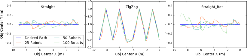
Figure 5: Trajectory taken by the centroid of the object vs the desired path in the three benchmarking paths.

Results We assess the performance of the algorithm observing the time taken to cage the object and push it along the benchmark paths, plotted in Fig. 6. The time to cage the object increases with the perimeter of the object: the median times to cage are $247\text{\,}\mathrm{s}779\text{\,}\mathrm{s}2753\text{\,}\mathrm{s}$ for $2550100$ robots, respectively transporting objects of size $\{2,2\}$, $\{3.6,6\}$, $\{7.2,12\}$. The 3 irregular shapes took around $300\text{\,}\mathrm{s}$ to cage when using 30 robots. The time taken to push the object is approximately $100\text{\,}\mathrm{s}$ for the straight path (regardless of the object size) and about $160\text{\,}\mathrm{s}$ for the zigzag with $2550$ robots.

When using 100 robots for the straight line and the zigzag, the system was slightly faster, which could be explained by the higher cumulative force exerted by the robots. The time taken following a straight path with rotations increases sub-linearly with the number of robots with median times being $135\text{\,}\mathrm{s}155\text{\,}\mathrm{s}200\text{\,}\mathrm{s}$ for $2550100$ robots, respectively.

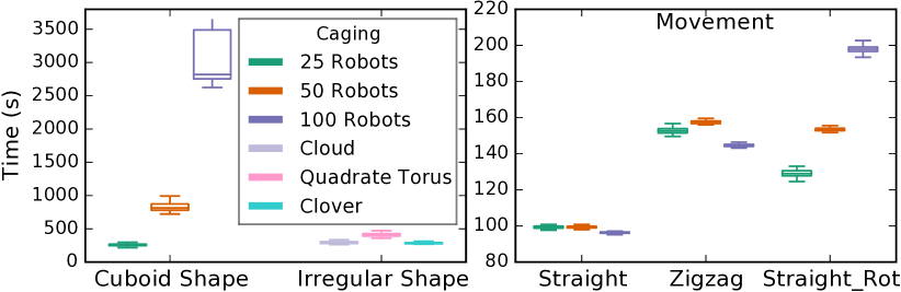
Figure 6: Time to complete caging (left) and push an object along 3 paths (right).

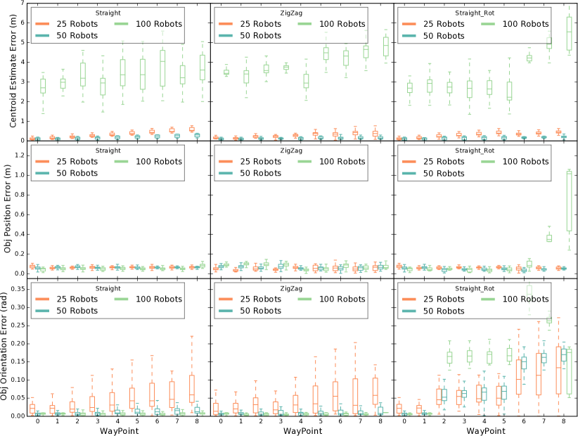
Figure 7: From top to bottom: the first plot shows the average centroid estimation error, the second shows the object centroid position error, and the third shows the object orientation error; from left to right, the figure shows the results for our 3 benchmark paths.

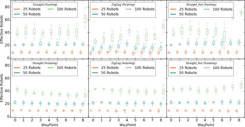
Figure 8: Number of robots that were effective in pushing and rotating at different waypoints of the three benchmark paths.

Fig. 7 shows the centroid estimation error, position error and orientation error on each row from left to right. The centroid estimation error increases as the robots progress along the path, which can be explained by the distortion in formation as the robots progress towards the final target. The centroid estimation error for 100 robots is relatively large and shows some variability, which could be largely influenced by the communication topology during the centroid estimation process, as detailed in sec. 3. The object position error computed using the difference between the desired position and the ground truth position appears stable around 0.1m, which is within our design tolerance ($d_{tol}$). In the $straight_{rot}$ case with 100 robots, the position error drastically increases around the final WPs, likely due to the drift induced by the second rotation. The orientation error accumulates slowly for the other paths, likely because the pushing force applied towards the target induces a small torque. Without global positioning, the error accumulates at every rotation.

Fig. 8 shows the number of effective robots for pushing and rotating the transported object, computed using 4. The number of effective pushers appears to increase slowly as the robots progress towards the final target in all cases, which could be due to distortions of the caging formation. The number of effective rotators stays constant for most of the cases, but increases during rotations, due to the robots either getting closer to the corners or the mid point of the object. This could be caused by the large error in the estimation of the centroid resulting in a generation of biased control input to rotate the object.

Robot Experiments We perform a small set of experiments using a group of 6 KheperaIV robots. The robots use a hub to compute and transmit the range and bearing information from a motion capture system, for more details on the experimental setup, we refer the reader to [22]. We performed two sets of experiments with robots transporting a foam box of size (0.285, 0.435)m: without any payload, and with $4\text{\,}\mathrm{kg}$ of LiPo battery on the object. Fig. 9 shows the trajectories followed by the robots and the inter-robot distance during the 3 runs without any payload and one run with the payload. It can be observed that the robots were able to consistently reach the target (0,0.9) by following the 3 WPs placed at every 0.3m. The inter-robot distance between the two adjacent robots in a cage approximates well the desired $I_{d}=0.45m$ at caging and it is maintained consistently during pushing in all runs with a maximum standard deviation of 0.1m.

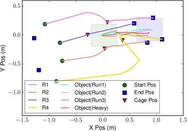
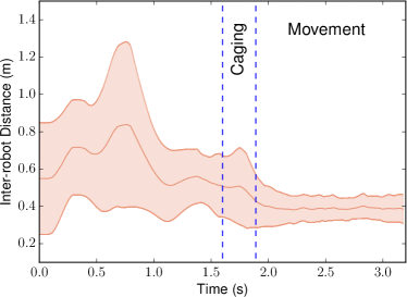
Figure 9: Trajectories taken by the robots (left) and the inter-robot distance between the two adjacent robot in the cage (right).

5 Conclusions

We propose a decentralized algorithm to cage an arbitrary-shaped object and transport it along a desired path consisting of a set of object poses. The robots periodically estimate the centroid of the object based on the positional information shared by the robots caging the object, and use this information to transport the object. We study the performance of our algorithm using a large set of simulation experiments with up to 100 robots traversing 3 benchmark paths and a small set of experiments on KheperaIV robots. As future work, we plan to implement a path planner to provide the object path in a cluttered environment.

References

- [1] Muhanad H Mohammed Alkilabi, Aparajit Narayan, and Elio Tuci. Cooperative object transport with a swarm of e-puck robots: robustness and scalability of evolved collective strategies. Swarm intelligence, 11(3-4):185–209, 2017.
- [2] Ramon S Melo B, Douglas G Macharet, Mario Fernandom M Campos, Ramon S Melo, Douglas G Macharet, and Mario Fernandom M Campos. Collaborative object transportation using heterogeneous robots. In Robotics, pages 172–191. Springer, 2016.
- [3] Jianing Chen, Melvin Gauci, Wei Li, Andreas Kolling, and Roderich Groß. Occlusion-Based Cooperative Transport with a Swarm of Miniature Mobile Robots. IEEE Transactions on Robotics, 31(2):307–321, 2015.
- [4] H. Choi, L. Brunet, and J. P. How. Consensus-based decentralized auctions for robust task allocation. IEEE Transactions on Robotics, 25(4):912–926, 2009.
- [5] Ryan Cotsakis, David St-Onge, and Giovanni Beltrame. Decentralized collaborative transport of fabrics using micro-uavs. In 2019 International Conference on Robotics and Automation (ICRA), pages 7734–7740. IEEE, 2019.
- [6] Yanyan Dai, YoonGu Kim, SungGil Wee, DongHa Lee, and SukGyu Lee. Symmetric caging formation for convex polygonal object transportation by multiple mobile robots based on fuzzy sliding mode control. ISA transactions, 60:321–332, 2016.
- [7] Jonathan Fink, Nathan Michael, and Vijay Kumar. Composition of vector fields for multi-robot manipulation via caging. In Robotics: Science and Systems, volume 3, 2007.
- [8] Antonio Franchi, Antonio Petitti, and Alessandro Rizzo. Distributed Estimation of State and Parameters in Multiagent Cooperative Load Manipulation. IEEE Transactions on Control of Network Systems, 6(2):690–701, 2019.
- [9] Chiara Gabellieri, Marco Tognon, Dario Sanalitro, Lucia Pallottino, and Antonio Franchi. A study on force-based collaboration in swarms. Swarm Intelligence, 14(1):57–82, 2020.
- [10] Aviram Gelblum, Itai Pinkoviezky, Ehud Fonio, Abhijit Ghosh, Nir Gov, and Ofer Feinerman. Ant groups optimally amplify the effect of transiently informed individuals. Nature Communications, 6, 2015.
- [11] Brian P Gerkey and Maja J Mataric. Pusher-watcher: An approach to fault-tolerant tightly-coupled robot coordination. In International Conference on Robotics and Automation (ICRA), volume 1, pages 464–469. IEEE, 2002.
- [12] Mehran Mesbahi and Magnus Egerstedt. Graph theoretic methods in multiagent networks, volume 33. Princeton University Press, 2010.
- [13] Guilherme A.S. Pereira, Mario F.M. Campos, and Vijay Kumar. Decentralized algorithms for multi-robot manipulation via caging. International Journal of Robotics Research, 23(7-8):783–795, 2004.
- [14] Kirstin H. Petersen, Nils Napp, Robert Stuart-Smith, Daniela Rus, and Mirko Kovac. A review of collective robotic construction. Science Robotics, 4(28), 2019.
- [15] Carlo Pinciroli and Giovanni Beltrame. Buzz: An extensible programming language for heterogeneous swarm robotics. In International Conference on Intelligent Robots and Systems, pages 3794–3800, October 2016.
- [16] Carlo Pinciroli, Adam Lee-Brown, and Giovanni Beltrame. A tuple space for data sharing in robot swarms. In Proceedings of the 9th EAI International Conference on Bio-inspired Information and Communications Technologies, BICT’15, pages 287–294, 2016.
- [17] Carlo Pinciroli, Vito Trianni, Rehan O’Grady, Giovanni Pini, Arne Brutschy, Manuele Brambilla, Nithin Mathews, Eliseo Ferrante, Gianni Di Caro, Frederick Ducatelle, Mauro Birattari, Luca Maria Gambardella, and Marco Dorigo. ARGoS: a modular, parallel, multi-engine simulator for multi-robot systems. Swarm Intelligence, 6(4):271–295, 2012.
- [18] Elon Rimon and Andrew Blake. Caging Planar Bodies by One-Parameter Two-Fingered Gripping Systems. The International Journal of Robotics Research, 18(3):299–318, 1999.
- [19] Ariel Rosenfeld, A Noa, O Maksimov, and S Kraus. Human-multi-robot team collaboration for efficent warehouse operation. Autonomous Robots and Multirobot Systems (ARMS), 2016.
- [20] Michael Rubenstein, Adrian Cabrera, Justin Werfel, Golnaz Habibi, James McLurkin, and Radhika Nagpal. Collective transport of complex objects by simple robots. Proceedings of the 2013 International Conference on Autonomous Agents and Multi-agent Systems, pages 47–54, 2013.
- [21] Michael Rubenstein, Alejandro Cornejo, and Radhika Nagpal. Programmable self-assembly in a thousand-robot swarm. Science, 345(6198):795–799, 2014.
- [22] V. S. Varadharajan, D. St-Onge, B. Adams, and G. Beltrame. Swarm relays: Distributed self-healing ground-and-air connectivity chains. IEEE Robotics and Automation Letters, 5(4):5347–5354, 2020.
- [23] Weiwei Wan, Rui Fukui, Masamichi Shimosaka, Tomomasa Sato, and Yasuo Kuniyoshi. Cooperative manipulation with least number of robots via robust caging. IEEE/ASME International Conference on Advanced Intelligent Mechatronics, AIM, pages 896–903, 2012.
- [24] Weiwei Wan, Boxin Shi, Zijian Wang, and Rui Fukui. Multirobot Object Transport via Robust Caging. IEEE Transactions on Systems, Man, and Cybernetics: Systems, 50(1):270–280, 2020.
- [25] Ying Wang and Clarence W de Silva. Cooperative transportation by multiple robots with machine learning. In 2006 IEEE International Conference on Evolutionary Computation, pages 3050–3056. IEEE, 2006.
- [26] ZhiDong Wang, Yasuhisa Hirata, and Kazuhiro Kosuge. Control a rigid caging formation for cooperative object transportation by multiple mobile robots. In IEEE International Conference on Robotics and Automation, 2004. Proceedings. ICRA’04. 2004, volume 2, pages 1580–1585. IEEE, 2004.
- [27] Zijian Wang, Sumeet Singh, Marco Pavone, and Mac Schwager. Cooperative Object Transport in 3D with Multiple Quadrotors Using No Peer Communication. Proceedings - IEEE International Conference on Robotics and Automation, pages 1064–1071, 2018.