Asymptotic Analysis of the Pauli Potential for Atoms

Abstract

ABSTRACT: Modeling the Pauli energy, the contribution to the kinetic energy caused by Pauli statistics, without using orbitals is the open problem of orbital-free density functional theory. An important aspect of this problem is correctly reproducing the Pauli potential, the response of the Pauli kinetic energy to a change in density. We analyze the behavior of the Pauli potential of non-relativistic neutral atoms under Lieb-Simon scaling – the process of taking nuclear charge and particle number to infinity, in which the kinetic energy tends to the Thomas-Fermi limit. We do this by mathematical analysis of the near-nuclear region and by calculating the exact orbital-dependent Pauli potential using the approach of Ouyang and Levy for closed-shell atoms out to element Z=976. In rough analogy to Lieb and Simon’s own findings for the charge density, we find that the potential does not converge smoothly to the Thomas-Fermi limit on a point-by-point basis but separates into several distinct regions of behavior. Near the nucleus, the potential approaches a constant given by the difference in energy between the lowest and highest occupied eigenvalues. We discover a transition region in the outer core where the potential deviates unexpectedly and predictably from both the Thomas-Fermi potential and the gradient expansion correction to it. These results may provide insight into semi-classical description of Pauli statistics, and new constraints to aid the improvement of orbital-free DFT functionals.

I Introduction

The most generally accurate and widely used method for predicting electronic structure is the Kohn-Sham (KS) approach to density functional theory (DFT). [1] By introducing auxiliary orbitals into the definition of particle density, the KS functional allows for an accurate representation of the energy of the exact many-body Hamiltonian by the energy of a simpler noninteracting system. [2, 3] This greatly simpliifies the mathematics and speeds up computations as compared to many-body or Hartee-Fock calculations. [4] However, the use of orbitals still comes with increasing computational cost as the number of particles in the system is up-scaled. This means that for systems that require the calculation of many orbitals such as mesoscale systems where quantum properties may be important[5] and warm dense matter, [6, 7, 8] in which many states become thermally activated, the computational cost of the KS method becomes prohibitive.

The Hohenburg-Kohn theorem, however, states that the ground state of any Hamiltonian system can be uniquely characterized by the particle density alone. [9] This means that exact Hamiltonian solutions can be expressed as functionals of exclusively the density, eliminating the need for orbitals.[4, 10] Crucially, this theorem applies to any piece of the energy, so not only is the true interacting Kinetic energy a functional of the density but also the KS kinetic energy: as conventionally defined, this is a functional of the KS orbitals, nevertheless a more general orbital-free expression should exist.

Recent years have seen a growing number of approaches to constructing orbital-free DFT (OFDFT) approximations to the KS method that allow for improved computational scaling for systems with large numbers of orbitals.[10, 11] The orbital-free philosophy has also been introduced successfully into conventional KS DFT, in the form of “de-orbitalizing” exchange-correlation functionals that depend explicitly upon the KS kinetic energy density (KED), replacing it with an equivalent expression in terms of the density and its derivatives. [12]

However the challenge of developing a robust OFDFT model with reasonable predictive accuracy for a variety of systems is severe. In conventional Kohn-Sham DFT one needs to approximate the exchange-correlation energy describing the difference in energy between interacting and noninteracting systems for the same external potential, normally a small correction. OFDFT must approximate the kinetic energy, which is of the order of the energy itself and must therefore be modeled to high accuracy.

The most basic OF theory, Thomas-Fermi (TF) theory, [13, 14] uses the KE of the homogeneous electron gas applied to the local density, in analogy to the LDA of the KS method. But unlike the LDA, which produces at least qualitatively good structural predictions, TF theory does not permit chemical binding at all. [15, 16, 17] The simplest functional beyond Thomas-Fermi, the gradient expansion (GE), does very well for atoms, but still not so well for molecular binding. Many attempts have been made to build on this foundation to develop semilocal or “single-point” functionals using the local density and its gradient as ingredients, [18, 19, 20, 21, 22, 23, 24] sometimes adding the Laplacian of the density, [25, 26, 27, 28, 29] and the electronic Hartree potential. [30] These more complex models generally share the problems of their predecessors, but can be competitive [28] with more expensive empirical nonlocal functionals for some solids.

Two-point nonlocal functionals have been somewhat more successful. [31, 32, 33] These are based on the Lindhard formula for linear response of the homogeneous electron gas. However, the Lindhard function is not an appropriate reference point for finite systems and systems with surfaces. [34] At least to date, such functionals require system-dependent empirical parameters to succeed.

The challenge of OFDFT is modeling the kinetic energy due to the Pauli exclusion principle – the orbital dependence in the KS functional is a consequence of Pauli statistics. One considers the total kinetic energy as a sum of this Pauli KE contribution and the von Weizsäcker KE – the KE of a fictitious Bose system with the same density as the real system. Minimizing the OFDFT energy then generates an Euler equation for the density for this fictitious Bose system where the contribution of Pauli statistics appears as an effective Pauli potential, that forces this fictitious system to have the same density as the true fermionic one. This Pauli potential thus is analogous to the Kohn-Sham potential for the conventional Kohn-Sham method.

The Pauli potential thus plays an important role in guaranteeing the stability and accuracy of structural calculations; nonetheless, like the Kohn-Sham potential, it gets much attention in developing functionals than the Pauli energy. A notable exception to this tendency is the use of the non-negativity of the potential as a constraint – a significant feature of at least one family of functionals. [22, 24] Nonetheless, a quite pleasing property of the exact Pauli potential is that it can be easily constructed in terms of KS orbitals in a simple fashion.[35] Essentially one can use the orbital definition of density to solve the KS problem and equivalent Euler problem simultaneously. This allows one to compare the results of model Pauli potentials to the exact potential for any system of interest. Exact Pauli potentials have been constructed in this way for example atoms, [35, 36, 37, 38, 39, 40] Approximate Pauli potentials play a key role in a recently developed OF method [17, 41, 40]. These rely on the orbitals of isolated atoms and an orbital-free description of the bond, thus constituting a hybrid approach to deorbitalizing the KS problem.

One way to generate useful constraints for functional development – whether on the total energy or the potential – is to consider the behavior of the functional under scaling of the system. A particularly fruitful example is Lieb-Simon scaling, the best known example of which is the scaling of the KE of neutral atoms as nuclear charge tends to infinity. [42, 43, 26] This should not be confused with Levy-Perdew scaling which more closely resembles the scaling of nuclear charge to infinity with constant particle number.[44] The lower bound of this scaling behavior is the von Weizsäcker (VW) solution for hydrogen and helium, trivially convertible to orbital-free form because it involves only one occupied orbital. The upper bound is less simple but more powerful. The leading order in $Z$ of the total and kinetic energy as $Z\to\infty$ is given by TF theory [42]. The gradient expansion approximaton (GEA) contributes corrections of smaller order in $Z$ to the large $Z$ limit of the energy. [43, 26] The limiting behavior of total energies is reflected in the kinetic energy density, which is locally approximated by a variant of the gradient expansion in the core region of the atom. [27]

The physical property that has not been explored carefully in the Lieb-Simon limit is the Pauli potential. Even though the total Pauli kinetic energy should be well described by TF theory in this limit, the same does not necessarily hold point for point for the potential. And it is unknown to what extent functionals that are successful in describing total energies work for the potential.

In this paper, we analyze the behavior of the exact KS Pauli potential for nonrelativistic neutral atoms as a function of $Z$ up to $Z=976$, large enough to extract limiting behavior and exact constraints that may be of aid to the development of KE functionals. We find an exact constraint in the near-nucleus limit and an unexpected deviation from the Thomas Fermi limit for a the outer shells of the large-$Z$ atom.

The paper is organized as follows: Section II discusses the theoretical background of Pauli potentials, both in the context of KS and of OFDFT approximations. Section III describes the methods and algorithms used for calculations and validation of the results. Section IV details the visual results of extending the exact Pauli response functionals and Pauli potentials to large-$Z$, as compared to approximations. Section V discusses the ramifications of our findings and possible future work.

II Theory

In Kohn-Sham theory, the total energy of an electronic system as a functional of the density $\rho$ is given by

$$E[\rho]=T_{KS}[\rho]+U[\rho]+\int v_{ext}(\bm{r})\rho(\bm{r})d^{3}r+E_{xc}[\rho],$$ (1)

where $T_{KS}[\rho]$ is the noninteracting contribution to the KE, $U[\rho]$ is the static electron-electron interaction, $v_{ext}$ is an external potential, and $E_{xc}$ is the energy of exchange and correlation effects. The last term contains the difference in energy between the true interacting system and the fictitious noninteracting one.

The KS density is given by

$$\rho(\bm{r})=\sum_{i}f_{i}|\phi_{i}(\bm{r})|^{2},$$ (2)

where $\phi_{i}$ are the auxiliary single-particle orbital that describe the noninteracting system and $f_{i}$ is the occupation number. The KS kinetic energy is then given by

$$T_{KS}=\int\tau_{KS}d^{3}r=\int\frac{1}{2}\sum_{i}f_{i}|\nabla\phi_{i}(\bm{r})|^{2}d^{3}r,$$ (3)

where $\tau_{KS}$ is a positive-definite kinetic energy density.

The density is determined by the functional minimization of the energy with respect to each orbital, with the constraint of preserving orbital normalization. This generates the effective Kohn-Sham equation for each orbital:

$$\left[\frac{1}{2}\nabla^{2}+v_{KS}(\bm{r})\right]\phi_{i}(\bm{r})=\epsilon_{i}\phi_{i}(\bm{r})$$ (4)

where $\epsilon_{i}$ is an auxiliary eigen value. The KS potential is determined from the functional derivative of the energy:

$$v_{KS}=\frac{\delta}{\delta\rho}\left(U[\rho]+E_{xc}[\rho]\right)+v_{ext}.$$ (5)

In order to generate an orbital-free version of the Kohn-Sham functional, we define the Pauli KE as the difference between KS and vW kinetic energies.

$$T_{p}=T_{KS}-T_{vW},$$ (6)

and define a Pauli KE density, the integral over which yields the Pauli KE, similarly:

$$\tau_{p}=\tau_{KS}-\tau_{vW}.$$ (7)

As discussed in the introduction, the vW kinetic energy, in the spirit of the KS idea, is the kinetic energy of a fictitious Bose system that has the same energy and density as the true, fermionic system. In this case, all particles occupy the ground state, $\rho=N|\psi_{0}|^{2}$, so that the associated KE density is

$$\tau_{vW}=-\frac{1}{2}\left|\nabla\sqrt{\rho(r)}\right|^{2}=\frac{1}{8}\frac{|\nabla\rho(\bm{r})|^{2}}{\rho(\bm{r})}.$$ (8)

This is strictly correct for the true system only if $N\leq 2$. The Pauli KE then measures the additional kinetic energy due to Fermi statistics. This has to be approximated somehow by a functional of the density, in a way similar to how the XC energy incorporating electron interactions is approximated in KS theory.

One can now generate an orbital-free Euler expression of the KS problem. It calculates the non-interacting Bose KE explicitly and considers effects of the Pauli contribution to the KE to come from a positive definite Pauli potential $v_{p}$. Minimizing $E-\mu\int\rho(\mathbf{r})d^{3}r$, one finds

$$\left[-\frac{1}{2}\nabla^{2}+v_{\mathrm{eff}}(\mathbf{r})\right]\sqrt{\rho(\mathbf{r})}=\mu\sqrt{\rho(\mathbf{r})}.$$ (9)

Like the KS procedure, this generates an effective potential $v_{\mathrm{eff}}$, and solves for the density and a single eigenvalue $\mu$, the chemical potential. The effective potential is given by $v_{\mathrm{eff}}=v_{KS}+v_{p}$, with the addition to the Kohn-Sham potential – the Pauli potential $v_{p}$ – given by[35]

$$v_{p}(\mathbf{r})=\frac{\delta T_{p}[\rho]}{\delta\rho(\bm{r})}.$$ (10)

It can be interpreted as the potential needed to make the density of the fictitious Bose system calculated with Eq. [9] equal the density of the fermionic Kohn-Sham system.

The Pauli potential may be determined exactly in terms of the KS orbitals as [35]

$$v_{p}(\mathbf{r})=\frac{\tau_{p}(\mathbf{r})}{\rho(\bm{r})}+v_{r}(\mathbf{r})$$ (11)

where $v_{r}$ is the response of the effective potential, and consequently the KE, to an arbitrary change in density. The exact response potential is given by [35]

$$v_{r}(\mathbf{r})=\frac{2}{\rho(\bm{r})}\sum_{j=1}^{M}(\epsilon_{M}-\epsilon_{j})\phi_{j}^{*}(\bm{r})\phi_{j}(\bm{r}).$$ (12)

Eq. 11 and 12 can be derived by simultaneously solving Eq. 4 and Eq. 9 using the same density Eq. 2 where the occupation $f_{i}=2$.

The primary tool for our study of atomic Pauli potentials is Lieb and Simon’s $\zeta$ scaling of the kinetic energy of neutral atoms [42, 45, 43, 26, 27]. The Lieb-Simon theorem scales the potential and particle number of a system simultaneously:

$$N_{\zeta} = \zeta N_{1},$$ (13)

$$v_{\zeta}(r) = -\frac{\zeta}{r}.$$ (14)

This yields the neutral atoms for integer values $Z$ of the continuous variable $\zeta$ with the choice $N_{1}=1$. Particle distance is then scaled in units of the Thomas-Fermi atomic radius $\sim Z^{-1/3}a_{0}$ so that formally, the potential scales as

$$v_{\zeta}=\zeta^{4/3}v_{1}(\zeta^{1/3}r).$$ (15)

The key result for this paper is that in the limit $\zeta\to\infty$, (for atoms, $Z\to\infty$) the total energy and thus also kinetic energy in the Thomas-Fermi approximation becomes relatively exact:

$$\lim_{\zeta\to\infty}\frac{T_{KS}-T_{TF}}{T_{KS}}\to 0.$$ (16)

Secondly, in the case of atoms, the TF energy and the leading corrections in the $Z\to\infty$ limit are exactly known and form an expansion in powers of $Z^{1/3}$:

$$T_{KS}=c_{0}Z^{7/3}+c_{1}Z^{2}+c_{2}Z^{5/3}+...$$ (17)

Here the leading order $c_{0}=0.768745$ is predicted by TF theory, [13] $c_{1}=-1/2$, [46, 47] and $c_{2}=0.269900$. [48] Any candidate for an orbital free KE functional ought to satisfy this scaling behavior, but this not a trivial task. [26] The second correction $c_{2}$ is generated by the standard gradient expansion. However, the Scott correction, which scales as $Z^{2}$, is a larger effect and although it may be modeled with a gradient expansion, it explicitly deals with the KE near the Coulomb singularity, where the GE is not legitimate. Not surprisingly, very few GGA’s or metaGGA’s get this limit correctly. [25, 26]

Given the importance of the gradient expansion model for the large $Z$ expansion, we will compare our results to functionals of this form; keeping in mind its limitations, we explore a number of variations on the theme. The leading order term of the large-$Z$ expansion is, as per Eq. (16), given by the the Thomas-Fermi KED [49] – the KED in the limit of a homogeneous electron gas, applied to the local density $\rho(\bm{r})$:

$$\tau_{TF}(\bm{r})=\frac{3}{10}k_{F}(\bm{r})^{2}\rho(\bm{r})=\frac{3}{10}(3\pi^{2})^{2/3}\rho(\bm{r})^{5/3}.$$ (18)

(It should be noted that this and subsequent model equations are defined for the Kohn-Sham and not the Pauli KED). The subsequent orders depend on the gradient expansion of the kinetic energy for the slowly varying electron gas. The gradient expansion may be formally derived as an expansion in orders of $\hbar$, good for large values of the local fermi energy – in effect, large numbers of occupied states. To second order it is given by [50]

$$\tau_{GEA}=\left[1+\frac{5}{27}p+\frac{20}{9}q\right]\tau_{TF},$$ (19)

where

$$p=\frac{|\nabla\rho|^{2}}{4{k_{F}}^{2}{\rho}^{2}},$$ (20)

and

$$q=\frac{\nabla^{2}\rho}{4{k_{F}}^{2}\rho}.$$ (21)

The fourth order [51] correction improves on this model for atoms [26, 52] but will not be considered in this paper.

Although this “canonical" GEA yields a reasonable description of the large $Z$ expansion, it is not perfect. It neither appears to be the best candidate for describing the total KE of atoms [26] nor the local KED. [53, 27] In fact, a modification of the GEA ($\mathrm{Loc}$) can be determined by fitting the local KED of the core shells of large-$Z$ atoms [27], which yields

$$\tau_{Loc}=\left(1-0.275p+2.895q\right)\tau_{TF}.$$ (22)

Although this does not yield good total energies, it is of obvious interest to model the potential which is also a local quantity and is related to the KED by Eq. 11. It is noteworthy that the gradient term of the $\mathrm{Loc}$ GE has a sign opposite to that of the canonical GE, and thus a net correction to the TF energy which is negative, rather than positive. Ref. 27 also introduces a $Z$-dependent near-nuclear correction to this that does yield good total energies, labelled $\mathrm{NNloc}$ in the results.

A similar local model is that of Lindmaa, Armiento and Mattsson, [53] given by:

$$\tau_{Airy}=\left[1-\frac{5}{27}p+\frac{30}{9}q\right]\tau_{TF},$$ (23)

This gradient expansion is derived from the analysis of the “edge electron gas" or Airy gas [54] that is constructed by taking a linear potential with hard wall boundary, in the limit that the hard wall is moved to infinity. Thus it is meant to be valid for surfaces, and not necessarily as global functional. It has been shown to be a good approximation for the KED of model systems including jellium droplets and the Bohr atom. As an atom is necessarily a system with a surface region, it is of interest to see how it fares here.

A final variant of the GE is introduced by Tsirelson et al. (Ref. 55) which uses an estimate of the chemical potential to modify the large-$r$ limit. The most relevant portion of their model is the response function which is fit to the following form:

$$v_{r,Ts}=\frac{(3\pi^{2})^{2/3}}{5}\rho^{2/3}+a\frac{|\nabla\rho|^{2}}{\rho^{2}}+b\frac{\nabla^{2}\rho}{\rho},$$ (24)

where $a=0.05$ and $b=0.14$.

We can now consider the functional derivative of the gradient expansion KE, to generate gradient expansion formulae for $v_{p}$ and $v_{r}$. The kinetic energy using second-order differentials of the density may be written as

$$T^{approx}_{KS}=\int\tau^{approx}_{KS}\left[\rho(\bm{r}),\nabla\rho(\bm{r}),\nabla^{2}\rho(\bm{r})\right]d^{3}r.$$ (25)

The functional derivative of this form is

$$\frac{\delta T^{approx}_{KS}}{\delta\rho}=\frac{\partial\tau_{KS}^{approx}}{\partial\rho}-\nabla\cdot\frac{\partial\tau_{KS}^{approx}}{\partial\nabla\rho}+\nabla^{2}\frac{\partial\tau_{KS}^{approx}}{\partial\nabla^{2}\rho}.$$ (26)

Now, consider an arbitrary second order GE of the form

$$T^{approx}_{KS}=\int\left(1+\eta_{Q}q+\eta_{P}p\right)\tau_{TF}\,d^{3}r$$ (27)

To get the Pauli KE, we subtract the von Weizsacker kinetic energy $\int(5p/3)\tau_{TF}\,d^{3}r$ from Eq. (27). Then applying the functional derivative [Eq. (26)] yields the GE approximation of the Pauli potential:

$$v_{p}^{GE}=\left[\frac{5}{3}+(\eta_{P}-5/3)p-2(\eta_{P}-5/3)q\right]\frac{\tau_{TF}}{\rho}.$$ (28)

which is independent of $\eta_{Q}$ because the Laplacian term $\sim q$ does not contribute to the KE or its functional derivative. The response function follows trivially from Eq. (11):

$$v_{r}^{GE}=\left[\frac{2}{3}-(\eta_{Q}+2(\eta_{P}-5/3))q\right]\frac{\tau_{TF}}{\rho}.$$ (29)

We finish by considering the regions of general behavior in atomic electron densities for large-$Z$ atoms proposed by the analysis of Lieb and Simon [42] and augmented by Heilman and Lieb. [56] Moving outward from the center, there is first a region near the nucleus where TF behavior breaks down, consisting of electrons whose behavior can be described described by the Bohr atom of non-interacting electrons. [56] There is an inner core region, the density of which should behave as a slowly varying electron gas obeying TF theory [Eq. (18)]. The characteristic length of this core scales as $Z^{-1/3}$ and the density scales as $Z^{2}$. There is a “mantle of the core" also with length scale $Z^{-1/3}$, and in which the density decays as $1/r^{6}$. In the infinite-$Z$ atom the ratio of electrons outside core and mantle to those inside drops to zero. Then, there is a “complicated transition region” [42] and a valence region of outer shells with a length scale presumably of order 1. Finally there is an evanescent region where the electron density decays exponentially. One check of how well we have approached the $Z\to\infty$ limit may be how many of these regions we can actually detect in our data.

III Methods

In order to calculate Kohn-Sham orbitals and eigenvalues needed for the calculation of exact KEDs and response potentials we use the atomic code FHI98PP[57] in its all-electron, non-relativistic mode. FHI98PP computes wave functions on a logarithmic grid, with spacing between successive points increasing by a geometric factor $\gamma$. We use the default $\gamma=0.0247$ which yields inappreciably different results from 0.0123. For simplicity, the exchange-correlation functional used was the PW91 LSDA.[58] The disagreement between LDA and exact Kohn-Sham calculations is known to disappear in the large-$Z$ limit; [43] in practice, our kinetic energies agree with exact OEP calculations within 0.67% for Ne and 0.055% for Rn. See Supplemental Material for further details. For differentiation of functions we employ Lagrange interpolating polynomials, similar to Gauss quadrature, with polynomials up to twelfth-order, while for integration we use the composite Simpson’s method. Details are given in Ref. 59.

The construction of extremely large atoms should also be discussed. For the nonrelativistic case, one naively extends the Aufbau principle out to infinity.[60] For atoms with highly degenerate valence energy shells, the lanthanum and actinium series for instance, this is likely a poor assumption, because completing such a shell might take preference over filling a lower energy shell with low degeneracy. However for atoms in the eight principal columns of the periodic table, all highly degenerate shells are already completely filled and thus do not influence the filling order.

We have extended FHI98PP using the Aufbau principle out to element number 976, with a 16p valence shell. The validity of this extension has been tested by comparing the total energy of Aufbau-constructed shells versus several other shell configurations for elements 976 (filled 16p), 970 (filled 15d), and 816 (filled 16s). For all cases tested, the Aufbau construction proves to be the nonrelativistic ground state for these atoms. To check the quality of our numerical solutions, completely independent calculations were done with a second atomic DFT code, OPMKS, [61] for atoms with $Z<400$. The results are indistinguishable with those of FHI98PP within machine error. A table of highest occupied atomic orbital (HOAO) eigenvalues and kinetic energies of large $Z$ atoms from both methods is given in the Supplemental Material.

IV Results

IV.1 Verifying densities

As a partial confirmation of our method, we compare densities generated by FHI98PP and the Aufbau principle for the mathematical element with $Z=976$ to the Thomas-Fermi density using the numerical parameterization of Ref. 26. Fig 1 shows the KS density (blue line), the TF density (red dotted line), and the TF limit of the density (black dotted line) versus scaled radius for element number 976. The scaling of $Z^{1/3}$ reflects the radius of the atom in the TF approximation, with peak radial density occurring for $Z^{1/3}r\sim 1$. Note the high agreement between the KS density and the TF density over a large range in scaled radius. However, though suppressed by the log plot, shell structure is evident in the KS density as oscillations around the TF density, wih the density deviating from the TF limit especially for the last oscillation or two ($Z^{1/3}r>10$). As expected the density diverges from the TF density for very large values of scaled radius, in the region of exponential decay beyond the last occupied shell. The Thomas-Fermi model assumes an infinite number of particles and continues indefinitely with the density decaying as $1/r^{6}$. The KS density never quite reaches the $1/r^{6}$ large-$r$ limit of the TF density (the “mantle” of the core of Ref. 42) and in this sense has not completely reached the TF limit.

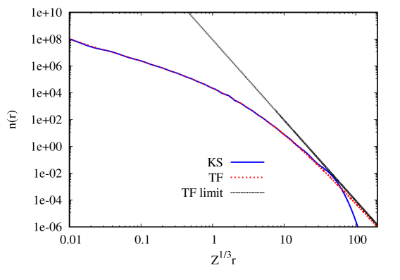
Figure 1: Comparison of KS density (KS), the TF density (TF), and the asymptotic TF limit (TF limit) for the Z=976 neutral atom.

IV.2 Pauli Potential: near the nucleus

As suggested by Lieb and Simon’s schema for describing the large-$Z$ atom, it is helpful to investigate Pauli potentials for separate regions of space. We thus examine first, the potential of the one or two electron shells nearest the nucleus, then that of the core and valence shells, and finally the evanescent behavior far from the nucleus. Fig 2 shows the Pauli potential and the two components that are used to construct it via Eq. (11) – the Pauli KED divided by the density and the response potential. The constant $\epsilon_{M}-\epsilon_{0}$ is shown as a solid red line.

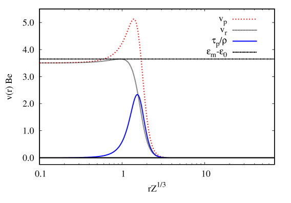
Figure 2: Various contributions to the Pauli potential for Be. Blue is the Pauli KED divided by the density, close black dotted is the response potential, and red dotted is the Paul potential. The eigenvalue difference $\epsilon_{M}-\epsilon_{0}$ between highest and lowest occupied orbitals is shown as a solid black line.

Beryllium is a usefully didactic system since it has only two shells – it is in effect a two-state system and the simplest atomic structure that has a non-zero Pauli contribution. The Pauli KED is nonzero only in the transition region between the 1s and 2s shells. Further out, it is zero because only the 2s shell effectively contributes to the KED – it becomes effectively a single state system indistinguishable from the bosonic case. Inside, the issue is more complicated. The 2s shell has a small nonzero piece and so naively one would expect the Pauli KED to be nonzero, but as we discuss in detail below, the Pauli KED is exactly zero at the nucleus as a consequence of the nuclear cusp condition on the density.

The response potential $v_{r}$ for Be is essentially a step function with a single step from the 1s shell, having an eigenvalue close to the hydrogenic 1s value, to the 2s shell. The second shell is the highest occupied energy shell and thus, given the definition of $v_{r}$ [Eq. (12)], makes zero contribution to the numerator of the response potential. The response potential of the lowest energy shell agrees reasonably well near the nucleus by the two-state energy difference $\epsilon_{M}-\epsilon_{0}=\epsilon_{2s}-\epsilon_{1s}.$[38]

The net effect on $v_{p}$ of the two contributions to it in Eq. (11) is instructive. Recall the conceptual definition of $v_{p}$: given a system of fermions in an external potential that one wishes to replace with a fictitous system of bosons with the same ground state density, then $v_{p}$ is the potential that one needs to add to the external potential in the bosonic system to achieve this. Here the goal is to make the density from a single bosonic state $\psi\sim\sqrt{\rho}$ duplicate the two shells of the fermionic system. This is done by creating a potential step (due to $v_{r}$) that pushes density out of the 1s shell region into the 2s shell region, while an additional barrier (due to $\tau_{p}/\rho$) separates the charge into two distinct shells. Finally, one may note that the values of $v_{p}$ and $v_{r}$ at contact with the nucleus are equal to each other and slightly less than $\epsilon_{M}-\epsilon_{0}$.

As there are known asymptotic behaviors for both total energy and near nuclear energy densities related with large Z scaling for the Kohn-Sham KE, it is of interest to analyze the large Z scaling of $v_{p}$. Fig 3 plots the same quantities as Fig 2, but for Rn. In addition we plot three gradient expansion models for the response potential discussed Sec II – the canonical GEA (purple dashed), the fit to the KED of high-Z atoms ($v_{Loc}$) (green dash), and the model of Ref. 55 (yellow dashed). Note that every potential visually has a three step structure with transitions at $Z^{1/3}r=0.1$ and $Z^{1/3}r=1$, related to the three innermost of six occupied shells (the remaining three shells are too small to see in this plot). In comparison to Be, $v_{r}$ seems to retain the step structure and $\tau_{p}$ has weak local maxima in between shells, but the shell structure overall is less pronounced.

Note that for Rn, $v_{p}$ is almost exactly $\epsilon_{m}-\epsilon_{0}$ in the near-nuclear region. This trend continues to improve as $Z\to\infty$, however visually Rn essentially shows complete agreement between $\epsilon_{m}-\epsilon_{0}$ and $v_{p}(r=0)$, so no larger Z atoms are plotted in this fashion. The actual contact value for $v_{p}(0)$ is much larger than that for Be – the energy scale is roughly $Z^{2}$, that of the noninteracting hydrogen-like system. At the same time $\tau_{p}(0)$ is definitely non-zero and so $v_{r}(0)$ and $v_{p}(0)$ are no longer the same value.

The GEA models all trend toward $-\infty$ as $\bm{r}\to 0$. This is due to the charge singularity at the origin, resulting in a Laplacian of the density that diverges in this limit. This is a flaw in any GEA model and is caused by the divergence term in Eq. (26). It is notable that the TS model does come close to predicting the turning point for $v_{r}$.

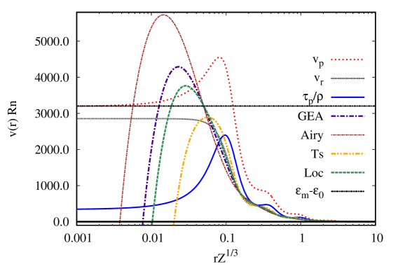
Figure 3: Components of the Pauli potential, $\frac{\tau_{p}}{\rho(\bm{r})}$, $v_{p}$, and $v_{r}$, for Rn, compared to response potential from several DFT models. GEA is the gradient expansion approximation [Eq. (19)], Airy, the Airy gas gradient expansion [Eq. (22)], loc, the fit to the local KED for high-$Z$ atoms [Eq. (23)], Ts, the Tsirelson model [Eq. (24)]. $\epsilon_{M}-\epsilon_{0}$ is difference between highest and lowest occupied eigenvalues.

IV.2.1 Analytic analysis of nuclear region

It seems from Fig. 3 that as $Z\to\infty$, the value of $v_{p}$ near the nucleus approaches a constant equal to $\epsilon_{M}-\epsilon_{0}$. At the same time, $\tau_{p}/\rho$ does not seem to converge to zero here, but rather to a value about 10$\%$ of $v_{p}(0)$; thus $v_{r}(0)$ falls short of $v_{p}(0)$ by the same amount. These asymptotic behaviors can be proven mathematically.

Naively, if one considers Eq. 12 as $\bm{r}\to 0$, and assume that the 1s orbital is the primary contribution to this equation, one gets

$$\lim_{r\to 0}v_{r}\approx(\epsilon_{M}-\epsilon_{0}).$$ (30)

This can not be exactly true because every s orbital has a contribution at the nucleus.

To improve the description, we consider what happens near the nucleus in the limit that nuclear charge $Z$ and electron number both go to infinity. Even for finite $Z$ the effect of electron-electron interactions becomes very small compared to the nuclear potential and thus they can be ignored. Low-lying energy eigenvalues approach in energy and degeneracy those of the corresponding noninteracting system – a Coulombic nuclear potential with charge $Z$. One thus can use hydrogenic wavefunctions to construct both $\tau_{p}$ and $v_{r}$ near the nucleus. This should be accurate out to a radius of order $r/Z$ where Lieb and Simon [42] show that the electron density starts to resemble that of the Thomas-Fermi atom.

To build a model for $v_{r}$ based on this picture we first note that for a hydrogenic central potential, the value at the nucleus of the radial component $R_{nl}$ of an eigenfunction is

$$R_{nl}(0)=\sqrt{4\left(\frac{Z}{n}\right)^{3}}\delta_{l0}.$$ (31)

Here the identity $L_{n-1}^{1}(0)=n$ for Laguerre polynomials has been used. Next, we apply this result to the exact expression for $v_{r}$ [Eq. (12)] by defining the net density of an angular momentum subshell,

$$\rho_{nl}(r)=\frac{(2l+1)}{4\pi}\left|R_{nl}(r)\right|^{2}$$ (32)

and, following Ref. 56, the density of a complete energy shell:

$$\rho_{n}(r)=\sum_{l=0}^{n-1}\rho_{nl}(r).$$ (33)

For a hydrogenic system, given the degeneracy in energy over angular momentum quantum number $l$, one has

$$v_{r}(r)=\sum_{n=1}^{M}\left(\epsilon_{M}-\epsilon_{n}\right)\rho_{n}(r)/\rho(r).$$ (34)

Since we are considering the limit $Z\to\infty$, it is appropriate also to take the limit that $M\to\infty$, that is, the perfect “Bohr atom” where all orbitals are filled and all are given by those of the noninteracting hydrogen atom. At the origin, only $l=0$ contributes, so $\rho_{n}(0)=\rho_{n0}(0)$. Thus Eq. (34) reduces to

$$v_{r}(0)=\braket{\epsilon_{n0}}={\displaystyle-\frac{\sum_{n=1}^{\infty}\epsilon_{n0}\rho_{n0}(0)}{\sum_{n=1}^{\infty}\rho_{n0}(0)}},$$ (35)

where we assume $\epsilon_{\infty}=0$. Substituting in Eqs. 32 and 31 and summing over $n$ gives

$$\rho(0)=\sum_{n=1}^{\infty}\frac{2}{\pi}\left(\frac{Z}{n}\right)^{3}.$$ (36)

Similarly, we use $\epsilon_{n}=-Z^{2}/2n^{2}$ for a hydrogenic atom and repeat this process to get the numerator of Eq. 35. With a bit of manipulation one can write the ratio as

$${\displaystyle v_{r}(0)={\frac{Z^{2}}{2}\frac{\zeta(5)}{\zeta(3)},}}$$ (37)

where

$$\zeta(s)=\sum_{n=1}^{\infty}{\frac{1}{n^{s}}}$$ (38)

is the Riemann-Zeta function. Given that $\zeta(5)=1.03692$ and $\zeta(3)=1.20205$, one has as $Z\to\infty$

$$v_{r}(0)=0.862626\frac{Z^{2}}{2}=-0.862626\epsilon_{0}.$$ (39)

The Pauli KED near the nucleus can be analyzed in a similar fashion, with more difficulty, since it necessarily involves derivatives of orbitals. It is fairly straightforward to show that the contribution of $s$-orbitals to the KS KED exactly equals the von Weizsacker KED in this region. In effect, this describes the connection between the cusp conditions near the nucleus obeyed by $s$-orbitals, and that of the total density. Somewhat counterintuitively, $p$-orbitals also have a nonzero contribution to the KS KED near the nucleus, both radially and from their nonzero angular momentum[27, 59, 62, 63]. It is the contribution from these orbitals that cause $\tau_{p}$ to be nonzero near the nucleus.

The Bohr atom model used here for $v_{r}$ has recently been used by Constantin et al. to analyze the large-$Z$ limit of $\tau_{p}$ at the nucleus. In this case, they show (Eq. (20) of Ref. 63)

$$\lim_{Z\to\infty}\tau_{p}(0) = \sum_{n=1}^{\infty}3\tau_{vW}[\rho_{n1}](0)$$ (40)

$$= \sum_{n=1}^{\infty}\frac{(n^{2}-1)Z^{5}}{\pi n^{5}},$$ (41)

where $\tau_{vW}[\rho_{nl}]$ is the vW KED evaluated using the density of the $(nl)$ angular momentum subshell. The end result is closely related to that for the $Z\to\infty$ limit of $v_{r}(0)$:

$$\frac{\tau_{p}(0)}{\rho(0)}=\frac{Z^{2}}{2}\frac{\zeta(3)-\zeta(5)}{\zeta(3)}$$ (42)

and therefore, using Eq. (11)

$$\lim_{Z\to\infty}v_{p}(0)=\frac{Z^{2}}{2}$$ (43)

This may be recast in a form that is more robust as well as conceptually revealing. First we note that the limit $Z^{2}/2$ is shared with the lowest orbital eigenvalue:

$$\lim_{Z\to\infty}\epsilon_{0}=-\frac{Z^{2}}{2}.$$ (44)

Then, observing that the form of the response potential involves a difference between the highest occupied eigenvalue $\epsilon_{M}$ and the other occupied eigenvalues, and noting that $\epsilon_{M}$ is a small energy independent of $Z$, we posit the general limit for $v_{p}(0)$:

$$v_{p}(0)\sim\epsilon_{M}-\epsilon_{0}.$$ (45)

We verify these assumptions first by plotting, in Fig. 4, ($\epsilon_{M}-\epsilon_{0})/Z^{2}$ (red dashed) and $-\epsilon_{0}/Z^{2}$ (blue) for alkali metals and noble gases from He to $Z=976$. These are plotted against the small parameter $Z^{-1/3}$ that characterizes the large-$Z$ expansion of atomic energies. We fit this trend with a polynomial form $(ax^{2}+bx+0.5)$ with $x=Z^{-1/3}$. A least squares regression results in $a\!=\!-0.879\pm 0.017$ and $b\!=\!-0.091\pm 0.004$. The fit is highly accurate for large Z atoms, starts to deviate from the observed around $Z<64$, but is still within 10% of the true value for Ne. One may note that dropping $\epsilon_{M}$ from the approximation for $v_{p}(0)$ affects the result primarily for He where in fact $\epsilon_{M}=\epsilon_{0}$. At the same time, the value of $-\epsilon_{0}$ is significantly off the hydrogenic value of 0.5 for any realistic value of $Z$.

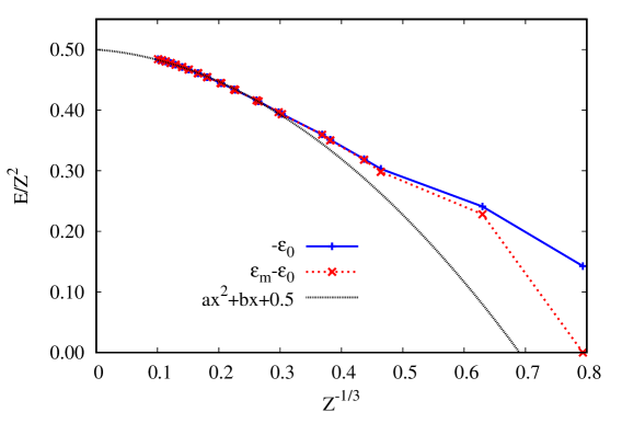
Figure 4: Analysis of lowest energy eigenvalue of large-$Z$ atoms versus the small parameter $Z^{-1/3}$ for the large-$Z$ expansion of atomic energies. We show $-\epsilon_{0}+\epsilon_{M}$, $-\epsilon_{0}$, and a curve fit of the form $ax^{2}+bx+0.5$ versus $x=Z^{-1/3}$ for noble gases from He to $Z=976$.

To test our assumptions of the finite-$Z$ value of $v_{p}(0)$ [Eqs. (43) and (45)] work, we next plot in Fig. 5 the value of $v_{p}-v_{r}$ (blue) at the origin for all atoms in columns 2, 13, and 18 of the periodic table, extended to $n=16$ ($Z=976$.) This is again scaled by $Z^{2}$ and plotted versus $Z^{-1/3}$. Subtracting off $v_{r}$ removes the large majority of the Pauli potential at the origin, leaving a relatively small piece (equal to $\tau_{p}/\rho$) which makes the error in our limiting ansatz readily visible. Then we compare to the difference between the large $Z$ limit $\epsilon_{M}-\epsilon_{0}$ and $v_{r}$ (black dashed line) and repeat for the the less accurate limit $-\epsilon_{0}$ (red dashed). Data is taken from three columns of the periodic table, and differentiated by plotting points of different types. A complete table of data used to generate fig. 4 and fig. 5 /is included in supplemental materials.

Note that all three functions of Z approach the same limit as $Z\to\infty$, converging to less than 1% error in $v_{p}(0)$ by roughly $Z=36$. Furthermore this dependence is column independent– curves from each column plotted fall onto the same trend after just one shell. This makes sense since we are measuring the Pauli potential at the nucleus, where presumably the effects of a variably filled valence shell should be minimal. The effect of including $\epsilon_{M}$ in our model is felt most for single-shell systems like He, where it retrieves the exact value of zero for $V_{p}(0)$. We make a parabolic fit of the data to the trend $cx^{2}+dx+0.07$ where $x=Z^{1/3}$ (black dash-dotted line). A least-squares regression of our data at large $Z$ results in $c=-0.223\pm 0.009$ and $d=-0.0491\pm 0.0024$. The value of 0.07 for the $y$ intercept is determined using Eq. 42. The fit has a very weak linear term, indicating that the contact value of $v_{p}$ roughly varies with nuclear charge as $0.5Z^{2}+cZ^{4/3}$.

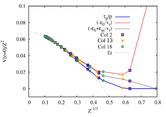
Figure 5: Contact values for $\tau_{p}/\rho$, $-\epsilon_{0}-v_{r}$, and $\epsilon_{M}-\epsilon_{0}-v_{r}$ as a function of $Z^{-1/3}$. Values taken atoms from columns 2 and 13 and 18 respectively, extended to $Z=976$, and compared to a parabolic fit $cx^{2}+dx+0.07$.

IV.3 Core and Valence

Next we consider the behavior of the Pauli potential and its constituents $\tau_{p}/\rho$ and $v_{r}$, away from the nucleus. For the ease of visualization across many shells, we employ unitless, scale-invariant quantities. For the kinetic energy density, it is common to do so by defining an enhancement factor, $F$, relative to the Thomas-Fermi KED:

$$F=\tau_{KS}/\tau_{TF}$$ (46)

and equivalently, a Pauli enhancement factor defined by

$$\tau_{p}=F_{p}\tau_{TF}$$ (47)

so that $F_{p}$ is given by

$$F_{p}=\left(\tau-\tau_{vW}\right)/\tau_{TF}.$$ (48)

For any model for the Kohn-Sham kinetic energy density, model Pauli enhancement factors may be similarly defined. Beyond the obvious advantages of scale invariance, the Pauli enhancement factor for the KS KED is closely related to the Electron Localization Factor (ELF) [64] and is equal to the $\alpha$ term used in meta-GGA functionals. [65, 66] In order to produce a unitless representation of the Pauli potential and its components, we scale each quantity by $\tau_{TF}/\rho$, the ratio of KE and particle densities in the TF model. This is $3/5$ of the local fermi energy $\epsilon_{F}$ in the TF picture.

Fig. 6(a) plots the Pauli enhancement factor $F_{p}$ for the Kohn-Sham KE density of radon. This is compared to various GE approximations: the standard gradient expansion, the Airy gas model [53], the local fit to the gradient expansion of Ref. 27 and the model of Ref. 55. These are plotted against the scaled distance $x=Z^{1/3}r$, chosen so that the peak radial probability density in the TF model for any atom occurs at roughly $x\!=\!1$. The constant line at one shows the TF limit for $F_{p}$.

A notable feature of these plots is the nearly periodic oscillation of the exact KE density and the GE models about the TF limit. This behavior reflects the shell structure of the atom: a value of $F_{p}<1$ indicates a region dominated by a single shell, producing a value for $\tau_{KS}$ lower than that predicted by TF theory, while the opposite is true for $F_{p}>1$. Thus each minimum indicates a different principal quantum shell. The five maxima show the regions of transition between the six shells of Rn, while the last exponentially divergent tail at large $r$ is the classically forbidden evanescent region outside the atom. It is interesting the oscillations have a roughly equal period in a semi-log plot, suggesting exponential growth in the period of quantum oscillations.

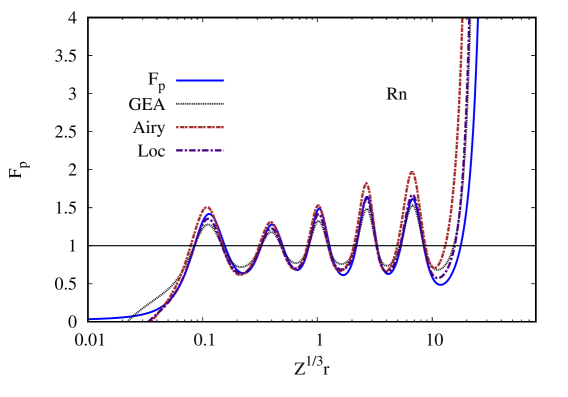
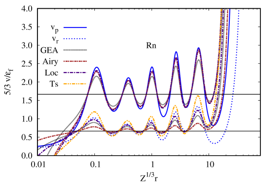
Figure 6: Unitless representation of KE potentials for radon. (a) Pauli enhancement factor $F_{p}$ for the Kohn Sham KED, compared to several variations of the gradient expansion approximation, versus scaled radius $Z^{1/3}r$. Models shown are the standard gradient expaonsion (GEA), Airy gas model (Airy), fit to the local KED of atoms (Loc) and the Tsirelson model (Ts); the Thomas-Fermi limit is shown as the solid horizontal line. (b) Pauli potential $v_{p}$ (solid blue line), response potential $v_{r}$ (dashed blue line), and gradient expansion approximations of the same, scaled by $\tau_{P}/\rho$. Each model is shown with the same color and dashing for $v_{p}$ and $v_{r}$ but center on different TF limiting cases – 5/3 for the former, 2/3 for the latter.

All versions of the gradient expansion recover the main qualitative features of the Pauli enhancement factor away from the nucleus and for the most part are quite accurate quantitatively. The quantum oscillations of the Tsirelson model start to deviate from the TF limit in the outer three shells; also the Airy gas model overestimates the true enhancement factor by a scaling factor of roughly 10/9.

Fig. 6(b) plots unitless representations of the Pauli potential $\rho v_{p}/\tau_{TF}$ and response potential $\rho v_{r}/\tau_{TF}$ versus scaled radial distance $Z^{1/3}r$ for radon. These are compared to various gradient expansion models, as before. The Pauli potential is not plotted for the Tsirelson model because of its dependence on the functional derivative of other quantities like exchange and correlation. Referring to Eqs. (28) and (29), we see that the Thomas-Fermi limit of the scaled Pauli potential is the constant 5/3, and that of the response potential, 2/3, shown as black horizontal lines.

Note that the scaled potentials show the same shell structure as the Pauli enhancement factor, oscillating about their TF limis with peaks and minima in nearly the same locations. The center of the oscillations starts to deviate from the TF line slightly for the outer three shells. This trend is better matched by the “non-canonical” GE’s like the Loc and Airy models than by the standard GEA.

Comparing gradient expansion models for the Pauli potential [Fig. 6(b)] we note that the Loc and Airy gas models outperform the conventional GE over most of the atom. Notably, the gradient expansion of the Pauli potential [Eq. (28)] only depends upon the coefficient $\eta_{P}$ for the contribution of the gradient expansion from the gradient variable $p[\rho(r)]$. Thus this data supports the use of a negative $\eta_{P}$ coefficient, as in the Airy gas and Loc models, in contrast to the positive coefficient of the standard gradient expansion. In addition the a priori Airy gas potential is almost as good as the empirically fit Loc model. At the same time, only the Loc model provides a close fit for the separate pieces of the Pauli potential, $\tau_{p}/\rho$ and $v_{r}$ (the Airy gas model is particularly poor for $v_{r}$, which underestimates the size of quantum oscillations by a factor of 3). Thus Loc has the best description of the coefficient $\eta_{Q}$ of the Laplacian term of the expansion.

We now consider the trends in atomic data as $Z$ is taken to be as large as practical in order to try to piece out the high-$Z$ limit. Fig 7, similarly to Fig 6 (b), plots the unitless representation of $v_{p}$ and $v_{r}$, as compared to various GE approximations, for element 976. This is the “noble gas” for row 16 of the periodic table mathematically extended using the Aufbau principle – thus there are 16 oscillations and 16 shells. Gratifyingly, these oscillations have considerably less amplitude than for radon, indicating passage towards the high-$Z$ limit. Note that although the inner eight shells of $v_{p}$ and $v_{r}$ oscillate about the TF limit, there is now an unmistakable trend away from the TF limit in the outer shells. This deviation is markedly absent in all the gradient expansion models. The deviation seems to be linear, and does not start until the middle shell of the atom is reached, around $Z^{1/3}r=1$. The last oscillation in the potential, demarcating the valence shell, occurs at $Z^{1/3}r\approx 40$. Similar plots are made for the Column 2, 10 and 13 atoms from row 16 in the Supplemental Material.

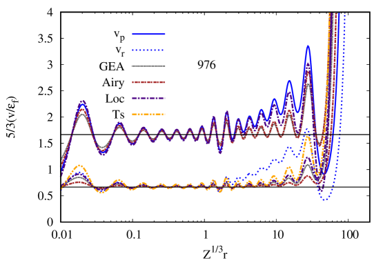
Figure 7: Unitless representation of the Pauli potential $v_{p}$, response potential $v_{r}$, gradient expansion approximation of the response potential $GEA$, Airy gas response potential $Airy$, the local variation of the GEA response potential $loc$, and the Tsirelson response potential $Ts$ for element 976.

To investigate further this unexpected behavior, we show in Fig. 8 the error in the Pauli enhancement factor $F_{p}^{model}-F_{p}^{exact}$ for the various GEA models, for the $Z=976$ atom. This highlights the “non asymptotic” piece in $F_{p}$ – the part that has not yet converged to the Thomas-Fermi asymptote. The scaled Pauli energy density $F_{p}$ shows no unexpected behavior whatsoever. The non-asymptotic remnant can be fit extremely well by a zero line, and its amplitude of oscillation is quite small. This is consistent with the Lieb-Simon theorem that the kinetic energy, obtained by integrating over the KE density must tend to the Thomas-Fermi limit for large $Z$.

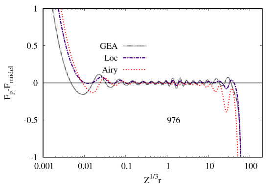
Figure 8: Difference between the exact Pauli enhancement factor $F_{p}$ and various GEA models for element 976, as function of scaled radius.

In contrast, Fig. 9 plots the difference between the exact response potential and the standard GEA approximation [Eq. (19)] for noble gas elements with even principle quantum number $n$ up to $Z=976$. The odd rows left out show a similar trend but with oscillations out of phase with the those of even rows. The deviation from the TF limit seen in Fig. 7 here forms part of a trend, apparent at radon and growing consistently with $Z$, along a linear trendline versus $\log(Z^{1/3}r)$, from about $Z^{1/3}r\!=\!2$ out to the edge of each atom. As $Z$ increases, the potential does not converge to the Thomas-Fermi limit – rather it deviates further away from it along this limiting trend. The valence shell (the last dip and peak before each curve drops to negative infinity) deviates from the trend of the inner shells. However it forms its own predictable linear trend away from the GE prediction, starting perhaps with Kr, with same slope as the inner shells.

The difference between the exact response potential and the standard GEA model for element 976 was fitted to a form $y=a\log(x/x_{0})$ for $x\!=\!Z^{1/3}r$ and $y\!=\!\rho v_{r}/\tau_{TF}$. The results of a linear regression are $a=0.194\pm 0.007$ and $x_{0}=1.39\pm 0.06$. In comparison, $x=a_{TF}=0.88$ is the position of peak radial density for the TF atom. An overall model of deviation from the TF limit can thus be extracted:

$$v_{r}(r)=v_{r}^{GEA}(r)+0.194\frac{\tau_{TF}}{\rho}\log{(Z^{1/3}r/1.39)}$$ (49)

A similar fit performed for $v_{p}$ yields results that agree within the fit standard deviation. (Details of the fit of the anomalies in $v_{p}$ and $v_{r}$ can be found in the Supplemental Material).

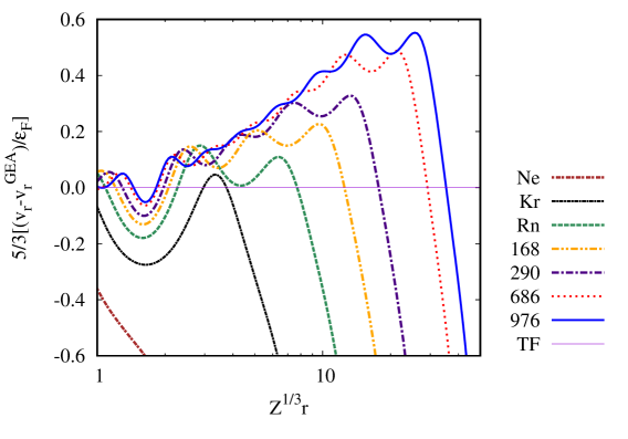
Figure 9: Scaled difference between $v_{r}$ and GEA response potential for noble gases with even principle quantum numbers up to $n=16$. The Thomas Fermi limit (TF) is narrow purple line; Ne, brown dashed; Kr, black dashed; Rn, green dashed; element 168, gold dot-dashed; 290, purple dot-dashed; 460, black dotted; 686, red dotted; and 976, blue solid.

It is worthwhile to analyze this deviation in terms of the scaled gradient and Laplacian of density in this region. One would expect these to become small nearly everywhere as $Z\to\infty$ and the total energy tends to the TF limit, but our results with the potential call this expectation into question. To this end, Fig. 10 shows parametric plots of the scale-invariant quantities $p(\bm{r})$ vs $q(\bm{r})$ for noble gases with even principle quantum numbers. Parametric plots for other large-$Z$ atoms can be found in the Supplemental Material.

There are three clear regions of behavior in this plot.[59, 27] The asymptotic approach of $q(\bm{r})\to-\infty$ indicates the nuclear cusp. The tail where $p(\bm{r})$ and $q(\bm{r})$ both tend to infinity indicates the evanescent region far from the atom. The loops or “orbits” come from the atomic core, reflecting the oscillations in $F_{p}$ and $v_{p}$ seen in Figs.  6 and 7. Each orbit represents a new shell, with $p$ and $q$ moving outwards to their largest values in regions between shells, and approaching the TF limit $p\!=q\!=0$ in the center of each shell. Thus one loop is seen for Ne with two shells. For increasing $Z$ one may in general see most loops shrinking towards $p\!=q\!=0$, indicating that the TF limit is being approached locally. But surprisingly, the process stops for the outermost loop, starting with radon. Subsequently this outer loop, formed by the valence shell and transition to the next shell is largely invariant with atomic number. A second loop seems largely stabilized by $Z=168$, and so on. For element 976, the inner shells are all close to the TF limit. However the outer orbitals gradually deviate from the TF limit, and show no sign of ever converging to this limit as $Z\to\infty$. So the deviation from the TF limit of $v_{r}$ for $Z^{1/3}>1$ is indicated by a similar deviation in the GE variables, suggesting that the GE will never become accurate for these shells. Similar behavior can be seen for other columns of the periodic table, with considerable differences in the last shell or two – data for columns 2, 12 and 13 of the periodic table are shown in the Supplemental Material.

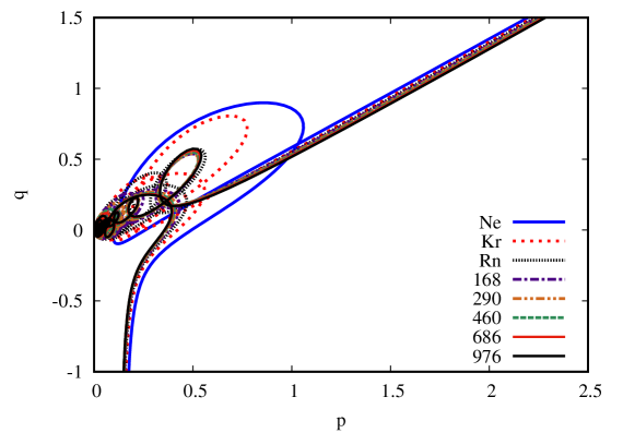
Figure 10: Parametric plot of $q(r)$ versus $p(r)$ for noble gas atoms with even principle quantum numbers.

It is interesting to note that Eq 9 implies that

$$v_{p}=\mu-v_{KS}-v_{vW},$$ (50)

where $v_{vW}=\frac{\delta T_{vW}}{\delta\rho}$ and $\mu\sim 0$ may be taken for a large-$Z$ atom. This implies that the unexpected behavior in the Pauli potential ought to mirrored in the KS potential as well. We find that this is indeed the case, calculating the XC potential using the Leeuwen-Baerends exchange potential [67], and the Perdew-Zunger LDA correlation potential [68]. The combined Hartree plus XC potential veers off the TF limit of $-5\tau_{TF}/3\rho$, to nearly cancel the Pauli potential, with each piece contributing about half of the net effect. The vW contribution does not show any unexpected behavior.

IV.4 Evanescent Region

Fig. 11 allows one to examine the evanescent region more closely. It plots the response potentials for elements 976 (red), 971 (black), 970 (blue), and 816 (gold), that is, the atom for column 2, 12, 13 and 18 for the 16th row of the extended nonrelativistic periodic table. Elements 976 and 971 both have p shells as their highest occupied atomic orbital (HOAO) and tend asymptotically to infinity. Elements 970 and 816 both have s shells as their HOAO and tend to zero. (Thus elements with s shells as their HOAO lack the last local minimum in $v_{r}$ present in the other cases.) The same trends are shown by the Pauli potential and the Pauli enhancement factor $F_{p}$.

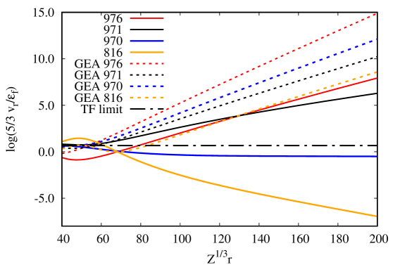
Figure 11: Evanescent behavior of $v_{r}$ for the alkali atom ($\!=\!816$), closed d shell atom (970), column 13 atom (971), and noble gas atom (976) with highest principle quantum number 16, as well as the GEA for each (dotted lines).

The standard GEA to the response potential for each element is shown with the same color and a dashed line. Other GE-like models (Loc, Airy gas) make very similar predictions. Note that the GEA shows roughly the same limiting behavior regardless of the column of the periodic table. They make reasonably accurate predictions for elements that have p shells as their HOAO but completely fail for the others.

One can partly explain the asymptotic trend of $v_{r}$ as $r\to\infty$ with a simple analysis of Eq. 12. The highest energy shell that contributes to an atom with $M$ shells is the $M-1$ shell. Defining $\rho_{M}$ as the density of the $M$-th energy shell, the assumption that $\rho(r)\approx\rho_{M}(r)$ as $r\to\infty$ gives the following approximation:

$$\lim_{r\to\infty}\frac{\rho(r)v_{r}(r)}{\tau_{TF}(r)}\approx\frac{2(\epsilon_{M}-\epsilon_{M-1})\rho_{M-1}(r)}{[\rho_{M}(r)]^{5/3}}.$$ (51)

The slope of the asymptotic behavior of Fig. 11 should thus be predicted by the logarithm of this result. The long-range exponential decay constant for the HOAO orbital is proportional to the square root of its eigenvalue, $\sqrt{2|\epsilon_{M}|}$, and this dominates the behavior of the density in the evanescent region. [69] A reasonable expectation for the decay constant for the second HOAO, at least for the local or semilocal exchange models employed in most DFT’s is, $\sqrt{2|\epsilon_{M-1}|}$. [70] In this case, the roughly linear behavior in Fig. 11 can be explained by a decay rate $\kappa\sim\sqrt{|\epsilon_{M-1}|}-(5/3)\sqrt{|\epsilon_{M}|}$, as shown in Table 1. The predicted rates agree closely with the observed behavior in Fig. 11. In general, the main predictor of the evanescent rate is whether the HOAO and second HOAO have the same or different principal quantum numbers. The former case leads to a $v_{r}$ that dies off slowly and tends to infinity relative to the local fermi energy $\sim\tau_{TF}/\rho$, while the latter case shows the opposite effect. Finally we note that the same qualitative trend in asymptotic behavior occurs for the full Pauli potential and the additional term $\tau_{P}/\rho$ that contributes to it, despite centrifugal terms [71] that contribute to these quantities.

Table 1: The two highest eigenvalues ($\epsilon_{M}$ and $\epsilon_{M-1}$) belonging to the HOAO and second HOAO states respectively, and the predicted exponential decay rate $\kappa$, for atoms in the 16th row of the extended periodic table. Negative $\kappa$ indicates exponential growth.

Atom	$\epsilon_{M}$	$\epsilon_{M-1}$	$\kappa$
816	-0.0859	-0.4004	0.1443
970	-0.1389	-0.4110	0.0199
971	-0.0928	-0.1827	-0.0802
976	-0.2113	-0.3572	-0.1685

V Discussion and Conclusions

In this paper, we have mapped the behavior of Pauli potentials of closed-shell atoms up to $Z=976$ or 16 complete energy shells. This represents a partial traversal of Lieb-Simon scaling to infinite $Z$, a process that transforms the Hamiltonian and expectations of real atoms to a limit where Thomas-Fermi theory is relatively exact for energies. Unlike energy expectations, expectations that are functions of position – the electron density and, in this paper, the Pauli potential – do not have to go to the Thomas-Fermi limit uniformly, and the electron density is richly structured even in the Thomas-Fermi limit. We find that this is true of the Pauli potential as well.

In comparison to the six regions of the large-$Z$ limit of electron density defined by Refs. 42 and  56, we can identify in our results perhaps five:

1. There is a near-nuclear region of constant Pauli potential.

2. An inner core region consisting of half of the occupied energy shells where the potential oscillates about the TF limit.

3. An outer core region, where the potential experiences an unexpected departure from the TF limit.

4. A small valence region where the last oscillation occurs, where the potential deviates slightly from the anomalous trend, varying somewhat between columns of the periodic table.

5. An evanescent region that also varies for each column of the periodic table. The slope of this evanescent region is related to the eigenvalues of the last two shells.

Notably, the $1/r^{6}$ limiting behavior of the TF atom density is just barely hinted at for the largest atom we study. The Lieb-Simon limit is understandably harder to reach for local features like the Pauli potential than for globally integrated quantities like the kinetic energy.

In the near-nuclear region (1) we find a constraint on the Pauli potential, analogous to that on the Pauli KED found in Ref. 71. The Pauli potential in the limit $r\to 0$ tends to the difference between the highest and lowest occupied eigenvalues. This result is consistent with the interpretation of the OFDFT Euler equation [Eq. (9)] as solving for the density of a system of fictitious bosons constrained to have the same density as the true fermionic system. Then the action of the Pauli potential in this region is to shift the energy of ones fictitious bosonic system from the lowest energy level of the actual fermionic system to that of the chemical potential $\mu$. It is interesting that the response potential in this region is nearly constant. Using the theorems of Ref. 56, it should be possible to prove that the slope of the response potential and thus the Pauli potential is zero at the nucleus.

The inner core shells are the only region where the Pauli potential clearly tends to the Thomas-Fermi limit as $Z\to\infty$. It is well fit by the gradient expansion in whatever variant, with the best candidate being the Loc GEA, which was fit to the KED in this region. This helps justify this model because KED by itself is ambiguously defined – it is the total energy and the potential that are the physical measurables of the system. The key point for an optimal fit seems to be a negative value to the coefficient for the $s^{2}$ term in the expansion – the Airy gas model with a similar negative coefficient performs about as well. Nevertheless, the fact that all variants of the gradient expansion work nearly equally well tells us that the dominant contribution of the Pauli potential comes from the removal of the von Weizsäcker KE from the Kohn-Sham kinetic energy. In fact, having no gradient correction at all, i.e., a Thomas-Fermi energy, would produce quite a good Pauli potential for atoms, if the real density could be used. That is, the Thomas-Fermi energy is not so much the problem here as the Thomas-Fermi density.

For outer half of the core, there is a surprising deviation from the TF limit as the system is scaled to large $Z$. This effect grows with $Z$ in a consistent way even as the size of quantum oscillations decreases, indicating that the potential in the Lieb-Simon limit diverges from the TF potential. This process seems not to be an artifact of numerical methods, and since it involves half of the energy shells, cannot depend much on minor errors in the Aufbau principle for determining the order of occupying the outermost shells.

The fact that the trend occurs over nearly half of the shells suggests a clue as to the origin of this effect. Within the Aufbau principle, the inner core is composed of energy shells that are completely filled; that is, all possible angular momentum subshells of a given quantum number are filled. The outer core shells are incrementally less complete, and the shells become dominated by orbitals with large numbers of radial nodes. The system structurally slowly trends from a fully three-dimensional, homogeneous gas, and towards something like the radial variant of a one-dimensional gas. In fact, if we associate each oscillation in the Pauli potential with a separate energy shell, the observed discrepancy is linear in the number of unoccupied angular momentum subshells for that energy. This is zero for the first roughly half of the energy shells of a noble gas atom, and increases linearly with each shell beyond that – exactly the behavior observed here.

This deviation also raises an interesting issue – does the Lieb-Simon limit for the total energy have a local equivalent for the potential, and if so where? For the large-$Z$ atom, it is common knowledge that the density diverges from the TF limit at the nucleus and asymptotically. Our work indicates that there is a finite but not ignorable deviation of the Pauli potential for a finite fraction of electrons.

The final, evanescent region is poorly described by all GE approximations. The response function for normal DFT models has a dependence upon the difference between the two highest energy eigenvalues that leads to an extreme range of asymptotic behaviors for the Pauli potential. The GE, is, at best, roughly comparable to the behavior of atoms with a $p$-shell valence and fails to capture the asymptotic trend of any other system.

There are a number of potential avenues along which to take this work further. One obvious track is to model the various deviations of the Pauli potential from the GE prediction in large-$Z$ atoms. A good question would be how to implement the near-nucleus constraint defined in Sec. IV.2. This does not seem possible in a standard semilocal or one-point model for the Pauli kinetic energy, at least using only the local density, gradient and Laplacian. It may be possible however to construct an accurate correction that explicitly depends on the nuclear charge $Z$ in the spirit of Ref. 62. Such a correction could not be easily made self-consistent, but might be worth the loss of self-consistency to produce a physically reasonable potential in this region.

Secondly, deriving a GGA model for the deviation of the Pauli potential from the TF limit in the outer core would be of interest, since this region is more directly involved in bonding. Preliminary calculations indicate that including fourth-order gradient expansion terms or simple generalized gradient approximations fail to reproduce the anomalous trend in the potential found for the outer half of the core shells. Such models can improve the potential in the outermost shell of the atom, which may be useful for improving binding, but do not capture the physics of the atom as a whole. The most intractable region to model seems to be the evanescent region, since the asymptotic behavior of the response potential depends on the eigenvalue spectrum. But this sensitivity is partly an artifact of the character of DFT orbitals – the asymptotic behavior of HF and higher-rung DFT orbitals depends upon the HOMO eigenvalue only, which may simplify the task for OFDFT considerably.

Finally, it would be of considerable interest to extend this study to relativistic systems. [72] We have studied nonrelativistic atoms because of the well-known large-$Z$ limiting behavior for this case. For relativistic systems, spin-orbit coupling spreads out eigenvalues with the same principal quantum number and grows more important as $Z$ increases. For the largest-$Z$ atoms fabricated in the lab, such as Oganesson, it is believed that this effect kills shell structure altogether in the outer core. [73] As this leads to a more homogeneous density, one might expect less deviation of the Pauli potential from the the Thomas-Fermi limit in this region than what we report here. In contrast, we expect that the basic physics underlying the value of the Pauli potential near the nucleus would be unaltered by relativistic corrections. The Pauli potential should still be given by the difference in energy between highest and lowest occupied eigenvalues, although of course these would be very different in value from the nonrelativistic case.

Supplementary Material

See supplementary material for tables and plots of kinetic energies using various models discussed in the paper; fits for the outer core of Pauli and response potentials and additional $p$ versus $q$ parametric plots. Additional data is available on request.

The author would like to thank Sam Trickey and Kieron Burke for helpful discussions, Eberhard Engel for use of his atomic DFT code, OPMKS, and Thomas Baker for help with the intricacies of gnuplot.

References

- Kohn and Sham [1965] W. Kohn and L. J. Sham, Phys. Rev. 140, A1133 (1965).
- Martin [2004] R. M. Martin, Electronic Structure: Basic Theory and Practical Methods (Cambridge University Press, 2004).
- Pribram-Jones, Gross, and Burke [2015] A. Pribram-Jones, D. A. Gross, and K. Burke, Annual Review of Physical Chemistry 66, 283 (2015).
- Karasiev, Chakraborty, and Trickey [2013] V. Karasiev, D. Chakraborty, and S. Trickey, “Progress on new approaches to old ideas: Orbital-free density functionals,” (2013).
- Akimov and Prezhdo [2015] A. V. Akimov and O. V. Prezhdo, Chemical Reviews 115, 5797 (2015).
- Graziani et al. [2014] F. Graziani, M. P. Desjarlais, R. Redmer, and S. B. Trickey, eds., Frontiers and Challenges in Warm Dense Matter, Lecture Notes in Computational Science and Engineering, Vol. 96 (Springer International Publishing, Switzerland, 2014).
- Rosner, Hammer, and Rothman [2010] R. Rosner, D. Hammer, and T. Rothman, “Basic research needs for high energy density laboratory physics, report on the workshop on high energy density laboratory physics research needs, nov. 15–18, 2009,” Tech. Rep. (US Department of Energy, Washington, DC, 2010).
- Karasiev, Sjostrom, and Trickey [2012] V. V. Karasiev, T. Sjostrom, and S. B. Trickey, Phys. Rev. B 86, 115101 (2012).
- Hohenberg and Kohn [1964] P. Hohenberg and W. Kohn, Phys. Rev. 136, B864 (1964).
- Tran and Wesolowski [2013] F. Tran and T. A. Wesolowski (2013).
- Witt et al. [2018] W. C. Witt, B. G. del Rio, J. M. Dieterich, and E. A. Carter, Journal of Materials Research 33, 777 (2018).
- Mejia-Rodriguez and Trickey [2018] D. Mejia-Rodriguez and S. B. Trickey, Phys. Rev. B 98, 115161 (2018).
- Thomas [1927] L. H. Thomas, Mathematical Proceedings of the Cambridge Philosophical Society 23, 542 (1927).
- Fermi [1927] E. Fermi, Rend. Acc. Naz. Lincei 6 (1927).
- Teller [1962] E. Teller, Rev. Mod. Phys. 34, 627 (1962).
- Xia et al. [2012] J. Xia, C. Huang, I. Shin, and E. A. Carter, The Journal of Chemical Physics 136, 084102 (2012).
- Finzel [2018] K. Finzel, Computational and Theoretical Chemistry 1144, 50 (2018).
- Tran and Wesolowski [2002] F. Tran and T. A. Wesolowski, Int. J. Quantum Chem. 89, 441 (2002).
- Lacks and Gordon [1994] D. J. Lacks and R. G. Gordon, J. Chem. Phys. 100, 4446 (1994).
- Thakkar [1992] A. Thakkar, Phys. Rev. A 46, 6920 (1992).
- Constantin et al. [2011] L. A. Constantin, E. Fabiano, S. Laricchia, and F. Della Sala, Phys. Rev. Lett. 106, 186406 (2011).
- Karasiev et al. [2013] V. V. Karasiev, D. Chakraborty, O. A. Shukruto, and S. B. Trickey, Phys. Rev. B 88, 161108 (2013).
- Borgoo, Green, and Tozer [2014] A. Borgoo, J. A. Green, and D. J. Tozer, Journal of Chemical Theory and Computation 10, 5338 (2014).
- Luo, Karasiev, and Trickey [2018] K. Luo, V. V. Karasiev, and S. B. Trickey, Phys. Rev. B 98, 041111 (2018).
- Perdew and Constantin [2007] J. P. Perdew and L. A. Constantin, Phys. Rev. B 75, 155109 (2007).
- Lee et al. [2009] D. Lee, L. A. Constantin, J. P. Perdew, and K. Burke, J. Chem. Phys. 130, 034107 (2009).
- Cancio and Redd [2017] A. C. Cancio and J. J. Redd, Molecular Physics 115, 618 (2017), https://doi.org/10.1080/00268976.2016.1246757 .
- Constantin, Fabiano, and Della Sala [2018] L. A. Constantin, E. Fabiano, and F. Della Sala, The Journal of Physical Chemistry Letters 9, 4385 (2018).
- Constantin, Fabiano, and Della Sala [2017a] L. A. Constantin, E. Fabiano, and F. Della Sala, Journal of Chemical Theory and Computation 13, 4228 (2017a).
- Constantin, Fabiano, and Della Sala [2017b] L. A. Constantin, E. Fabiano, and F. Della Sala, Journal of Chemical Theory and Computation 13, 4228 (2017b).
- Wang, Govind, and Carter [1999] Y. A. Wang, N. Govind, and E. A. Carter, Phys. Rev. B 60, 16350 (1999).
- Huang and Carter [2010] C. Huang and E. A. Carter, Phys. Rev. B 81, 045206 (2010).
- Mi, Genova, and Pavanello [2018] W. Mi, A. Genova, and M. Pavanello, The Journal of Chemical Physics 148, 184107 (2018).
- Constantin [2019] L. A. Constantin, Phys. Rev. B 99, 155137 (2019).
- Levy and Ou-Yang [1988] M. Levy and H. Ou-Yang, Phys. Rev. A 38, 625 (1988).
- Gritsenko, van Leeuwen, and Baerends [1994] O. Gritsenko, R. van Leeuwen, and E. J. Baerends, The Journal of Chemical Physics 101, 8955 (1994), https://doi.org/10.1063/1.468024 .
- van Leeuwen, Gritsenko, and Baerends [1995] R. van Leeuwen, O. Gritsenko, and E. J. Baerends, Zeitschrift fur Physik D Atoms Molecules Clusters 33, 229 (1995).
- Baerends and Gritsenko [1997] E. J. Baerends and O. V. Gritsenko, The Journal of Physical Chemistry A 101, 5383 (1997), https://doi.org/10.1021/jp9703768 .
- Kraisler and Schild [2020] E. Kraisler and A. Schild, Phys. Rev. Research 2, 013159 (2020).
- Finzel [2020] K. Finzel, Molecules 25 (2020), 10.3390/molecules25081771.
- Finzel [2019] K. Finzel, The Journal of Chemical Physics 151, 024109 (2019).
- Lieb and Simon [1973] E. H. Lieb and B. Simon, Phys. Rev. Lett. 31, 681 (1973).
- Burke et al. [2016] K. Burke, A. Cancio, T. Gould, and S. Pittalis, The Journal of Chemical Physics 145, 054112 (2016).
- Levy and Perdew [1985] M. Levy and J. Perdew, Phys. Rev. A 32, 2010 (1985).
- Lieb and Simon [1977] E. H. Lieb and B. Simon, Advances in Mathematics 23, 22 (1977).
- Scott [1952] J. Scott, Philosophical Magazine 43, 859 (1952).
- Schwinger [1980] J. Schwinger, Phys. Rev. A 22, 1827 (1980).
- Schwinger [1981] J. Schwinger, Phys. Rev. A 24, 2353 (1981).
- Spruch [1991] L. Spruch, Rev. Mod. Phys. 63, 151 (1991).
- Salasnich [2007] L. Salasnich, Journal of Physics A: Mathematical and Theoretical 40, 9987 (2007).
- Hodges [1973] C. H. Hodges, Canadian J. Phys 51, 1428 (1973).
- Jones and Gunnarsson [1989] R. O. Jones and O. Gunnarsson, Rev. Mod. Phys. 61, 689 (1989).
- Lindmaa, Mattsson, and Armiento [2014] A. Lindmaa, A. E. Mattsson, and R. Armiento, Phys. Rev. B 90, 075139 (2014).
- Mattsson and Kohn [2001] A. E. Mattsson and W. Kohn, The Journal of Chemical Physics 115, 3441 (2001), https://doi.org/10.1063/1.1396649 .
- Astakhov, Stash, and Tsirelson [2016] A. A. Astakhov, A. I. Stash, and V. G. Tsirelson, International Journal of Quantum Chemistry 116, 237 (2016), https://onlinelibrary.wiley.com/doi/pdf/10.1002/qua.24957 .
- Heilmann and Lieb [1995] O. J. Heilmann and E. H. Lieb, Phys. Rev. A 52, 3628 (1995).
- Fuchs and Scheffler [1999] M. Fuchs and M. Scheffler, Computer Physics Communications 119, 67 (1999).
- Perdew, Burke, and Wang [1996] J. P. Perdew, K. Burke, and Y. Wang, Phys. Rev. B 54, 16533 (1996).
- [59] J. J. Redd, “An analysis of atomic wave functions to improve density functional kinetic energy models,” Master’s thesis, Ball State University (2015).
- Pyykko [2011] P. Pyykko, Phys. Chem. Chem. Phys. 13, 161 (2011).
- Engel and Dreizler [1999] E. Engel and R. M. Dreizler, Journal of Computational Chemistry 20, 31 (1999).
- Acharya et al. [1980] P. K. Acharya, L. J. Bartolotti, S. B. Sears, and R. G. Parr, Proceedings of the National Academy of Sciences 77, 6978 (1980).
- Constantin, Fabiano, and Sala [2016] L. A. Constantin, E. Fabiano, and F. D. Sala, Computation 4, 19 (2016).
- Becke and Edgecombe [1990] A. D. Becke and K. E. Edgecombe, J. Chem. Phys. 92, 5397 (1990).
- Becke [1998] A. D. Becke, J. Chem. Phys. 109, 2092 (1998).
- Sun, Xiao, and Ruzsinszky [2012] J. Sun, B. Xiao, and A. Ruzsinszky, The Journal of Chemical Physics 137, 051101 (2012), https://doi.org/10.1063/1.4742312 .
- van Leeuwen and Baerends [1994] R. van Leeuwen and E. J. Baerends, Phys. Rev. A 49, 2421 (1994).
- Perdew and Zunger [1981] J. P. Perdew and A. Zunger, Phys. Rev. B 23, 5048 (1981).
- Morrell, Parr, and Levy [1975] M. M. Morrell, R. G. Parr, and M. Levy, The Journal of Chemical Physics 62, 549 (1975), https://aip.scitation.org/doi/pdf/10.1063/1.430509 .
- [70] This assumption is not true for orbitals derived from a scheme that involves the Fock operator, such as Hartree-Fock [74] or many-body quasiparticle orbitals. [75] In this case all orbitals are coupled to each other and all will have an asymptotic piece that decays like the HOAO. But our analysis holds for orbitals derived from any method such as a GGA or metaGGA which could presumably be used in an orbital-free context.
- Sala, Fabiano, and Constantin [2015] F. D. Sala, E. Fabiano, and L. A. Constantin, Physical Review B 91, 035126 (2015).
- Giuliani et al. [2019] S. A. Giuliani, Z. Matheson, W. Nazarewicz, E. Olsen, P.-G. Reinhard, J. Sadhukhan, B. Schuetrumpf, N. Schunck, and P. Schwerdtfeger, Rev. Mod. Phys. 91, 011001 (2019).
- Jerabek et al. [2018] P. Jerabek, B. Schuetrumpf, P. Schwerdtfeger, and W. Nazarewicz, Phys. Rev. Lett. 120, 053001 (2018).
- Handy, Marron, and Silverstone [1969] N. C. Handy, M. T. Marron, and H. J. Silverstone, Phys. Rev. 180, 45 (1969).
- Almbladh and von Barth [1985] C.-O. Almbladh and U. von Barth, Phys. Rev. B 31, 3231 (1985).