Abstract

We derive an approximate but explicit formula for the Mean First Passage Time of a random walker between a source and a target node of a directed and weighted network. The formula does not require any matrix inversion, and it takes as only input the transition probabilities into the target node. It is derived from the calculation of the average resolvent of a deformed ensemble of random sub-stochastic matrices $H=\langle H\rangle+\delta H$, with $\langle H\rangle$ rank-$1$ and non-negative. The accuracy of the formula depends on the spectral gap of the reduced transition matrix, and it is tested numerically on several instances of (weighted) networks away from the high sparsity regime, with an excellent agreement.

 

Contents

1. 1 Introduction
   1. 1.1 Setting and related works
   2. 1.2 Summary of main result
2. 2 Sketch of the proof
3. 3 Network examples
   1. 3.1 Fully Connected
   2. 3.2 Erdős-Rényi
   3. 3.3 Random Regular
4. 4 Conclusions
5. A Joint cumulant generating function for Gaussian $\delta h_{ij}$
6. B The accuracy of (5) and heterogeneous networks: the star graph case

 

1 Introduction

The exploration of a complex network by a walker that hops randomly from one node to another according to a given probabilistic rule has received much attention in recent years [2, 3, 5, 4, 1, 6, 7, 8, 9, 10, 11, 12, 13, 14, 15, 16, 17, 18, 19, 20], with many applications (see [21] for an excellent review), including the self-organization and generation of networks [22, 23, 24].

Among the most significant observables that can be studied analytically, the Mean First Passage Time (MFPT) plays a pivotal role. The MFPT is the average over many realizations of the walk of the “first-passage time” (or “first-hitting time”) – defined as the number of steps taken by the walker to reach a target node from a given source node for the first time. Applications range from biology [25, 26] to finance [27], ecology [28], kinetic network models [29] and many other fields (see [3, 30] for reviews on first-passage problems on networks and other media). More recently, the idea that the most “important” nodes should also be those that are most rapidly reachable by others has been used to rank constituents [31, 32, 33] and to assess heterogeneity and correlations [34] in complex networks.

The computation of the MFPT involves a cumbersome inversion of a reduced matrix of transition probabilities. For this reason, any analytical treatment of the MFPT has in general proven difficult, with a number of attempts made to derive exact expressions – often valid when transition matrices have special symmetries – as well as approximate and mean field results (see Sec. 1.1 for details). In particular, unveiling the connection between the structural properties of the underlying network and the MFPT – as well as its scaling properties – is a non-trivial task for the majority of network topologies [35].

In this paper, we address these issues by proposing an approximate but explicit formula for the MFPT of a walker on directed and weighted networks. Our formula does not require matrix inversions, it depends only on the local information about the target node, and sheds light on the interplay between structural and spectral properties of the underlying network.

The plan of the paper is as follows. In Section 1.1 we provide the main definitions and an overview of closely related literature, while in 1.2 we announce our main result. In section 2, we reproduce for completeness the main steps leading to the main formula (5) starting from a random matrix formulation of the problem, already outlined in [36, 37]. In section 3, we test our formula on different types of spectrally gapped (weighted) networks. Finally, in section 4 we offer some concluding remarks and outlook for future researches. The two Appendices are devoted to technical calculations and examples.

1.1 Setting and related works

Consider a weighted strongly connected network with $N$ nodes described by the (real valued, and not necessarily symmetric) adjacency matrix $A$. Given a source node $i$ and a different target node $j$, the MFPT $m_{ij}$ satisfies the following recurrence equation [38, 39, 40, 1]

$$m_{ij}=1+\sum_{\ell\neq j}^{N}T_{i\ell}m_{\ell j}\ ,$$ (1)

where the matrix element $T_{i\ell}$

$$T_{i\ell}=\frac{A_{i\ell}}{\sum_{r}A_{ir}}$$ (2)

encodes the transition probability of the walker from node $i$ to node $\ell$ (with $\sum_{\ell}T_{i\ell}=1$ for all $i=1,\ldots,N$ by normalization). The meaning of eq. (1) is straightforward: in its first step, the walker hops from node $i$ to node $\ell$, which produces the $+1$ on the right-hand side. Then, if the target has not been reached, we have to assign a weight to the MFPT from the “new” source node $\ell$ to the target $j$, which is the probability of reaching the “new” source node $\ell$ from the “old” source node $i$. This produces the second term on the right-hand side.

There are different strategies to extract meaningful information from (1). On the one hand, one could simply iterate the equation numerically – given the network instance and the diffusion protocol, encoded in the matrix $T$ – until convergence is reached [40]. Alternatively, for a given target node $j$, one could rewrite the equation in the vector-matrix form

$$\bm{m}^{(j)}=\bm{1}+T^{(j)}\bm{m}^{(j)}\Rightarrow\bm{m}^{(j)}=(\mathds{1}-T^{(j)})^{-1}\bm{1}\ ,$$ (3)

where all quantities are $(N-1)$-dimensional: $\bm{1}$ is the column vector of ones, $\mathds{1}$ is the identity matrix, and $T^{(j)}$ is the transition matrix where the $j$-th row and column have been erased [41]. The resulting vector $\bm{m}^{(j)}$ encodes all MFPT to the target node $j$ starting from all other nodes in the network. The seemingly harmless eq. (3) has however a few important drawbacks: (i) it requires the inversion of a possibly large and ill-conditioned matrix, which makes a numerical approach prone to inaccuracies [42], (ii) the nonlinear relation between $\bm{m}^{(j)}$ and $T^{(j)}$ makes it difficult to infer the functional dependence of the former on network parameters (e.g. the mean degree) from the knowledge of the latter – unless the transition matrix enjoys special symmetries or internal structure, and (iii) it implicitly takes for granted that the full adjacency matrix of the underlying network is known with great accuracy, which may not necessarily be the case in practical applications.

Another exact approach – pioneered by Noh and Rieger [43] – relies on the identity $m_{ij}=\sum_{n\geq 0}nF_{ij}(n)$, where $F_{ij}(n)$ is the probability that the walker starting from $i$ arrives in $j$ for the first time after $n$ moves. Using the Markov property of the walk, and suitable generating functions (see [21] for details) it is possible to write an expression for $m_{ij}$ in terms of the series coefficients of the (discrete) Laplace transform of $p_{ij}(n)$ – the probability that the walker starting in $i$ reaches $j$ after $n$ moves. Although exact, the final formula can be opaque to interpretations, unless the transition matrix has again special symmetries or structure that make the master equation analytically tractable [44]. These cases are a rare luxury, though.

Finally, there are a number of approximate results, using e.g. a mean-field approach [46, 47, 48, 45]. The crudest approximation consists in noticing that – regardless of the source node – the target node $j$ is reached with an approximate probability of $p_{j}^{\star}$ in each time step, where $\bm{p}^{\star}$ is the equilibrium probability vector of the Markov transition matrix. Therefore,

$$m_{ij}\approx\sum_{k=1}^{\infty}kp_{j}^{\star}(1-p_{j}^{\star})^{k-1}=\frac{1}{p_{j}^{\star}}\,.$$ (4)

The estimate in (4) can be rather loose, and $m_{ij}$ may deviate considerably from $1/p_{j}^{\star}$. More sophisticated mean-field approaches have been devised, which perform better in certain situations [49, 50, 45]. For discussion of scaling theory based on renormalization theory for first-passage time and other quantities on networks, see [52, 51]. For analytical approaches to MFPT based on spectral theory and generating functions, see [17, 53, 54, 55, 56, 57]. For other approaches and applications of first-passage times and return times on networks, see [58, 59, 60, 61, 62].

1.2 Summary of main result

In this paper, we put forward a novel approximate formula for $m_{ij}$, which we shall show in the following to be

$$m_{ij}\approx 1+(N-1)\frac{1-T_{ij}}{\sum_{\ell\neq j}T_{\ell j}}\ .$$ (5)

Our formula is valid on a generic (directed, weighted, strongly connected) network, provided that its reduced transition matrix $T^{(j)}$ – obtained by removing the $j$-th row and column – has a “large” spectral gap, defined as $\lambda_{1}-\max\{|\lambda_{2}|,\ldots,|\lambda_{N-1}|\}$ with $\lambda_{1}\in(0,1)$ the Perron-Frobenius eigenvalue, and the $\{\lambda_{i}\}$ being the other eigenvalues of $T^{(j)}$ in the complex plane. Since the spectral gap tends to diminish the sparser the network becomes [63, 64, 65], the formula (5) is not suitable for “too sparse” networks.

The formula (5) is strikingly simple, and – in spite of being obtained in a large-$N$ setting – we find that it is very accurate also for spectrally gapped walks on relatively small networks, as we demonstrate below. It is obtained by approximating the reduced transition matrix $T^{(j)}$ as a rank-$1$, sub-stochastic matrix: from each node $i\neq j$, the walker may either hop on $j$ directly (with probability $T_{ij}$), or hop on any of the other $N-1$ nodes – connected to $i$, or not – with the same probability $(1-T_{ij})/(N-1)$. Within this approximation, only the neighborhood of the target node really matters – which reveals an interesting approximate symmetry: two sufficiently dense networks that share the same set of transition probabilities into a given node $j$, also share the full set of MFPTs from any source node into the target $j$, irrespective of how “unlike” each other they are away from $j$. For simple diffusion on a fully connected network (where $T_{ij}=1/(N-1)$ for all $i\neq j$), our formula (5) reduces to the known (exact) result $m_{ij}=N-1$ – which holds true also for sufficiently dense Erdős-Rényi networks [66, 67], independently of the probability $p\sim\mathcal{O}(1)$ that each node pair has an edge between them. For a detailed discussion of results on MFPT on different kinds of graphs and fractal structures, see again [21] and references therein.

2 Sketch of the proof

In this section, we report for completeness the random matrix calculation that we outlined elsewhere [36, 37] in another context, from which the approximate formula (5) follows as an immediate corollary.

The main idea is to replace a given (empirical) reduced transition matrix $T^{(j)}$ with a random sub-stochastic matrix (called $H=(h_{\ell m})$ in the following), in such a way that “some” macroscopic features of $T^{(j)}$ are retained in $H$. More specifically, our model assumes that the row sums are preserved (on the average), i.e. $z_{i}:=\sum_{k}T^{(j)}_{ik}=\sum_{k}\Big{\langle}h_{ik}\Big{\rangle}$ – but these sums are spread “as evenly as possible” among the columns of $H$.

Consider therefore a random $N\times N$ matrix $H=(h_{\ell m})$ with $h_{\ell m}\geq 0$, which can be written as

$$H=\langle H\rangle+\delta H\ .$$ (6)

The deterministic rank-$1$ matrix $\langle H\rangle$ reads

$$\langle H\rangle=\begin{pmatrix}\frac{z_{1}}{N}&\cdots&\frac{z_{1}}{N}\\ \vdots&\ddots&\vdots\\ \frac{z_{N}}{N}&\cdots&\frac{z_{N}}{N}\end{pmatrix}$$ (7)

in terms of positive constants $\{z_{1},\ldots,z_{N}\}$. With this definition, the random matrix $H$ is essentially a “noise-dressed” version of the rank-$1$ (balanced) matrix $\langle H\rangle$, whose row sums are $\{z_{1},\ldots,z_{N}\}$. The entries – not necessarily independent – of the random perturbation $\delta H$ satisfy $\langle\delta h_{\ell m}\rangle=0$ for all $\ell,m$. The average $\langle\cdot\rangle$ is taken w.r.t. the joint probability density of the entries of the matrix $\delta H$.

Clearly, $\langle H\rangle$ has a single non-zero, real and positive eigenvalue $\lambda_{1}=\frac{1}{N}\sum_{\ell}z_{\ell}\equiv\bar{z}$, and $N-1$ zero eigenvalues – and therefore a spectral gap of $\sim\mathcal{O}(1)$. Assume that the spectral radius of $H$ satisfies $\rho(H)<1$.

If $\delta H$ were identically zero, the vector

$$\bm{m}=(\mathds{1}-H)^{-1}\bm{1}$$ (8)

could be computed exactly using the Sherman-Morrison formula [69] to give

$$m_{\ell}=1+\frac{z_{\ell}}{1-\bar{z}}\ ,$$ (9)

with $\bar{z}=(1/N)\sum_{i=1}^{N}z_{i}$.

In presence of a random perturbation $\delta H$, we ask what the average value of $\bm{m}$ would be,

$$\langle\bm{m}\rangle=\langle(\mathds{1}-H)^{-1}\bm{1}\rangle\ ,$$ (10)

and in particular how small should the perturbation $\delta H$ be to ensure that the Sherman-Morrison result (9) keeps holding on average – to leading order in $N$ – even in this “noise-dressed” case. It turns out that $\delta H$ must satisfy a certain cumulant decay law (see eq. (21) below). The condition on the spectral radius $\rho(H)<1$ ensures instead that the inverse matrix on the r.h.s. of (10) exists.

It is instructive to see what happens in the special case of an i.i.d. Gaussian perturbation with $\langle\delta h_{ij}^{2}\rangle=\sigma_{N}^{2}$ for all $i,j$, for which fuller analytical considerations are possible. Let us reverse momentarily the roles of $\delta H$ and $\langle H\rangle$. We would essentially have here a real Gaussian and non-symmetric matrix $\delta H$ (hence belonging to the Ginibre ensemble [70]), which is deformed by a rank-$1$ matrix $\langle H\rangle$. This problem – albeit with the additional twist that we require positivity of the final matrix – is relatively well-understood in Random Matrix Theory [71, 72, 73, 74]. In the absence of the rank-$1$ deformation, the spectrum of $\delta H$ would fill a circle in the complex plane with radius $r_{N}=\sqrt{N}\sigma_{N}$ – this is known as Girko-Ginibre circular law. However, the addition of the rank-$1$ deformation $\langle H\rangle$ leaves the circular bulk of eigenvalues unperturbed, but may lead to the appearance of an extra isolated outlier at $\lambda_{out}=\bar{z}\sim\mathcal{O}(1)$. Choosing “too big” a variance $\sigma_{N}^{2}$ has therefore two harmful effects: (i) positivity of the matrix entries of $H$ is no longer guaranteed, and (ii) all the eigenvalues of $H$ become of the same order, with the circular bulk swallowing up the outlier and annihilating the spectral gap. A similar clash between the positivity constraint (leading to a Perron-Frobenius outlier) and the standard circular law for Gaussian matrices – leading to a phase transition – was recently noted in [75].

In order to get a large spectral gap, we need to require

$$r_{N}=o(1)\Rightarrow\sigma_{N}=o(1/\sqrt{N})\ .$$ (11)

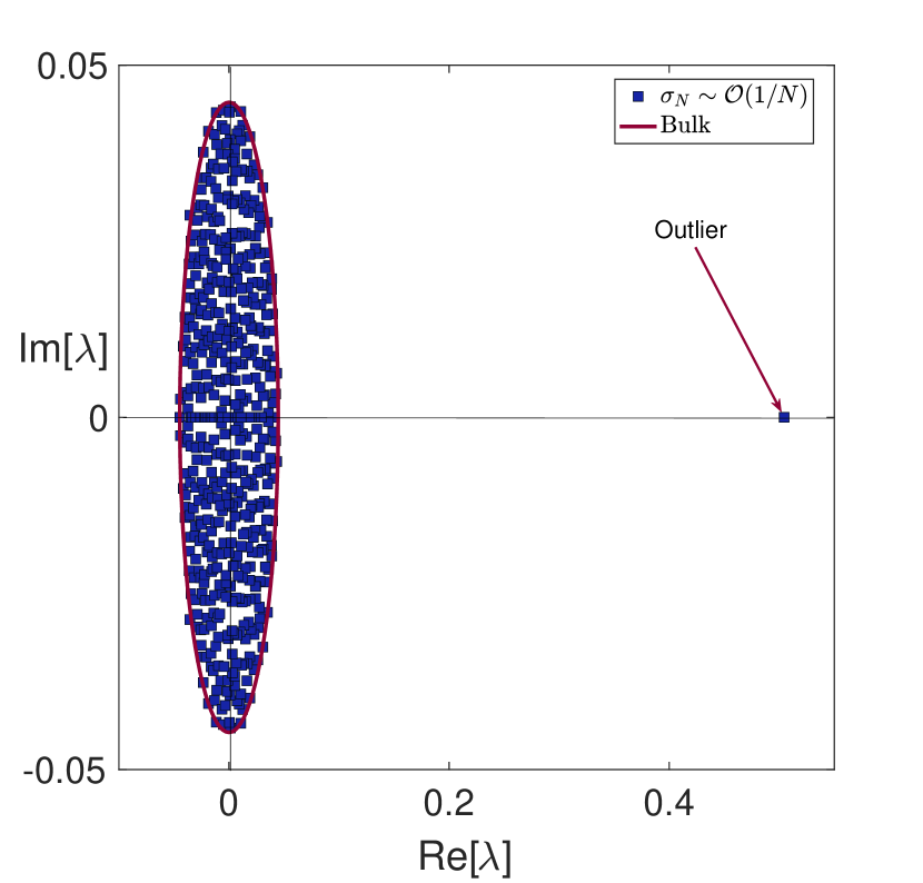
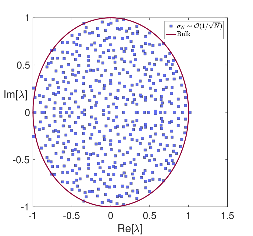
Figure 1: Left: Spectrum of a typical instance of a $N=500$ Gaussian matrix (with $\sigma_{N}\sim\mathcal{O}(1/N)$) plus a rank-$1$ deformation of the form (7). The red line encloses the circle of radius $r_{N}\sim\mathcal{O}(1/\sqrt{N})$, while an isolated outlier at $\lambda_{out}=\bar{z}$ is clearly visible. Right: Spectrum of a typical instance of a $N=500$ Gaussian matrix (with $\sigma_{N}\sim\mathcal{O}(1/\sqrt{N})$) plus a rank-$1$ deformation of the form (7). The red line encloses the circle of radius $r_{N}\sim\mathcal{O}(1)$, which swallows the would-be outlier at $\lambda_{out}=\bar{z}$ altogether. The same constant values $\{z_{1},\ldots,z_{N}\}$ have been used to produce the two plots.

In Fig. 1 we plot on the left the typical spectrum of a randomly generated matrix of the form (6), with i.i.d. Gaussian $\delta h_{ij}$ having $\sigma_{N}\sim\mathcal{O}(1/N)$, while on the right we have $\sigma_{N}\sim\mathcal{O}(1/\sqrt{N})$. One clearly observes that the relative fluctuation $\sigma_{N}/\langle H\rangle_{ij}$ is too large in the latter case to guarantee positivity and a large enough gap.

This simple numerical experiment – consistent with the analytical estimate in (11) – shows that a generic positive and sub-stochastic matrix (provided its spectral gap is “large”) can be interpreted as the superposition of a rank-1 matrix (fully determined by the original row sums) and a Gaussian noise matrix with sufficiently small variance. We will show in section 3 that such large-gap matrices appear naturally in the treatment of MFPT on weighted networks away from the high sparsity regime.

To compute (10), one first defines the $2N\times 2N$ Hermitian matrix

$$B(\eta)=\begin{pmatrix}-\mathrm{i}\eta\mathds{1}&\mathds{1}-H^{T}\\ \mathds{1}-H&-\mathrm{i}\eta\mathds{1}\end{pmatrix}\ ,$$ (12)

where $\mathrm{i}$ is the imaginary unit, and $\eta$ is a small regularizer that ensures that $B^{-1}$ exists.

Using the formula for the inverse of a block matrix, it is possible to show [37] that

$$\langle m_{\ell}\rangle=\lim_{\eta\to 0}\sum_{k=N+1}^{2N}\Big{\langle}[B^{-1}(\eta)]_{\ell,k}\Big{\rangle}\qquad\ell=1,\ldots,N\ .$$ (13)

Next, we use the following result: given a (complex) symmetric matrix $M$ of size $N\times N$, with purely imaginary diagonal elements $M_{ii}=-\mathrm{i}m_{ii}$, with $m_{ii}>0$, the following formula holds

$$[M^{-1}]_{ab}=\mathrm{i}\frac{\int\mathrm{d}\bm{x}~{}x_{a}x_{b}\exp\left[-\frac{\mathrm{i}}{2}\sum_{i,j}^{N}x_{i}M_{ij}x_{j}\right]}{\int\mathrm{d}\bm{x}\exp\left[-\frac{\mathrm{i}}{2}\sum_{i,j}^{N}x_{i}M_{ij}x_{j}\right]}\ ,$$ (14)

where $\bm{x}$ denotes a $N$-dimensional vector, and the integrals run over $\mathbb{R}^{N}$ [76].

Applying this formula to the $2N\times 2N$ matrix $B(\eta)$, and inserting it in Eq. (13), we get the following integral representation of the $\ell$-th element of the vector $\bm{m}$ in (10)

$$\langle m_{\ell}\rangle=-\mathrm{i}\lim_{\eta\to 0}\lim_{\bm{\omega},\bm{\xi}\to\bm{0}}\Big{\langle}\frac{Z_{1}(\bm{\omega},\bm{\xi},H)}{Z(H)}\Big{\rangle}\ ,$$ (15)

where

$$Z_{1}(\bm{\omega},\bm{\xi},H) =\sum\limits_{m=1}^{N}\partial_{\omega_{\ell}}\partial_{\xi_{m}}\int\mathrm{d}\bm{x}\mathrm{d}\bm{y}~{}\exp\left[-\frac{\eta}{2}\sum\limits_{i=1}^{N}(x_{i}^{2}+y_{i}^{2})-\mathrm{i}\sum\limits_{i=1}^{N}x_{i}y_{i}+\mathrm{i}\sum\limits_{i=1}^{N}\omega_{i}x_{i}\right.$$

$$\left.+\mathrm{i}\sum\limits_{i=1}^{N}\xi_{i}y_{i}+\mathrm{i}\sum\limits_{i,j=1}^{N}x_{i}h_{ji}y_{j}\right]$$

$$Z(H) =\int\mathrm{d}\bm{x}\mathrm{d}\bm{y}~{}\exp\left[-\frac{\eta}{2}\sum_{i=1}^{N}(x_{i}^{2}+y_{i}^{2})-\mathrm{i}\sum_{i=1}^{N}x_{i}y_{i}+\mathrm{i}\sum_{i,j}^{N}x_{i}h_{ji}y_{j}\right]\ .$$ (16)

Using the “replica trick” [77, 78, 79]

$$\frac{Z_{1}}{Z}=\lim_{n\to 0}Z_{1}Z^{n-1}\ ,$$ (17)

where the variable $n$ is initially promoted to an integer, we get rid of the denominator and land on

$$\langle m_{\ell}\rangle =-\mathrm{i}\lim_{n\to 0}\lim_{\eta\to 0}\lim_{\bm{\omega},\bm{\xi}\to\bm{0}}\sum_{m=1}^{N}\partial_{\omega_{\ell}}\partial_{\xi_{m}}\int\prod_{a=1}^{n}\mathrm{d}\bm{x}_{a}\mathrm{d}\bm{y}_{a}\exp\left[-\frac{\eta}{2}\sum_{i=1}^{N}\sum_{a=1}^{n}(x_{ia}^{2}+y_{ia}^{2})-\mathrm{i}\sum_{i,a}x_{ia}y_{ia}\right.$$

$$\left.+\mathrm{i}\sum_{i=1}^{N}\omega_{i}x_{i1}+\mathrm{i}\sum_{i=1}^{N}\xi_{i}y_{i1}\right]\Phi(\{\bm{x}_{a}\},\{\bm{y}_{a}\})\ ,$$ (18)

where

$$\Phi(\{\bm{x}_{a}\},\{\bm{y}_{a}\})=\exp\left(\frac{\mathrm{i}}{N}\sum_{i,j}^{N}z_{j}\phi_{ij}\right)\varphi\left(\{\phi_{ij}\}\right)$$ (19)

with

$$\varphi\left(\{\theta_{ij}\}\right)=\Big{\langle}\mathrm{e}^{\mathrm{i}\sum_{i,j}^{N}\delta h_{ji}\theta_{ij}}\Big{\rangle}$$ (20)

being the joint cumulant generating function of the entries of the matrix $\delta H$, and $\phi_{ij}=\sum_{a}x_{ia}y_{ja}\sim\mathcal{O}(1)$. Assuming the following cumulant decay condition

$$\log\varphi\left(\{\phi_{ij}\}\right)=o(N)$$ (21)

for large $N$, we can neglect all higher-order terms and land on a “replicated” version of the Sherman-Morrison formula for the matrix $\langle H\rangle$ alone, yielding eventually

$$\langle m_{\ell}\rangle=1+\frac{z_{\ell}}{1-\bar{z}}+o(1)\ ,$$ (22)

with $\bar{z}=(1/N)\sum_{i=1}^{N}z_{i}$.

In summary, provided that the cumulants of $\delta h_{ij}$ decay sufficiently fast for large $N$, the “noise-dressing” of the average, rank-$1$ matrix $\langle H\rangle$ is inconsequential, and the Sherman-Morrison formula is universal (noise-independent) to leading order in $N$. Although for the most general, arbitrarily correlated noise term $\delta H$ it is difficult to establish formally that the cumulant decay condition (21) is equivalent to $H$ having a “large” spectral gap, the intuition garnered from the Gaussian case leads us to conjecture this must be generally the case.

The formula (5) for the MFPT readily follows from the identification $H\equiv T^{(j)}$, and $z_{\ell}\equiv 1-T_{\ell j}$. This is due to $z_{\ell}$ being the (average) sum of the $\ell$-th row of $H\equiv T^{(j)}$, and $T^{(j)}$ being obtained by the row-stochastic matrix $T$ ($\sum_{k}T_{\ell k}=1$) by erasing the $j$-th row and column.

3 Network examples

In this section, we apply our formula to walks on different network instances (fully connected, Erdős-Rényi, random regular). More precisely, we now test Eq. (5) against (i) exact evaluations of formula (3) for the MFPT via direct matrix inversion, and (ii) numerical simulations of random walks. We do not report here on (dense) scale-free topologies, whose phenomenology is very similar to the other cases, albeit with significantly larger fluctuations: a detailed study of this (and other) heterogeneous cases is deferred to a separate publication. We do, however, test on a simple and exactly solvable case (the star graph with $N$ nodes) the hypothesis that the accuracy of our approximate formula (5) may vary (within the same instance) from node to node, depending on how well connected the target node is to the rest of the network (see Appendix B for details).

3.1 Fully Connected

We consider a single instance of a fully connected, directed, weighted network with $N=500$. Each link is endowed with a random weight sampled from a uniform distribution in $[0,1]$. In all cases below, we have checked that nothing changes with other edge weights (e.g. exponential). We fix a source node $i$ and a target node $j$, and we consider random walks starting in $i$ and hitting $j$ for the first time after $m_{ij}$ hops, performed according to the transition probabilities in Eq. (2). In Fig. 2 we see (i) a plot of the eigenvalue spectrum in the complex plane for a typical instance of the sub-stochastic matrix $T^{(j)}$, obtained erasing the $j$-th row and column from the original transition matrix $T$ defined in eq. (2), and (ii) a scatter plot of exact MFPT (eq. (3)) vs. our approximate formula (5) – each point in the plot refers to a randomly picked $(i,j)$ pair on a randomly generated instance of the graph. We observe that the points nicely follow the straight line with slope $1$.

To the best of our knowledge, at present there are no exact and explicit formulas available for the MFPT on a weighted and directed fully connected network, in spite of the very simple geometry of the system. Our approximate formula does an excellent job while requiring as input only the $N-1$ incoming weights into the target node $j$ – all the other information away from $j$ being entirely irrelevant. Indeed, given one instance $T$ of the transition matrix, we have constructed another synthetic instance $T^{\prime}$ such that – for a prescribed node $j$ – we have $T_{ij}=T^{\prime}_{ij}$ for all $i$. All the other entries in each row of $T^{\prime}$ are randomly reshuffled with respect to the corresponding row of $T$, to preserve the row sum constraint $\sum_{\ell}T_{i\ell}=\sum_{\ell}T^{\prime}_{i\ell}=1$. We have checked that the two walkers $T$ and $T^{\prime}$ share the full set of MFPTs into node $j$, as expected.

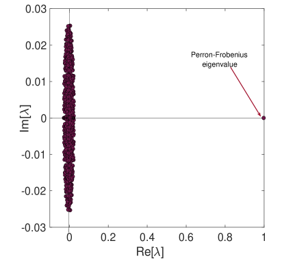
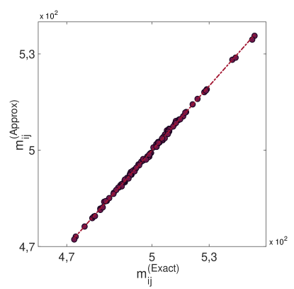
Figure 2: Left: eigenvalues in the complex plane for a typical instance of $T^{(j)}$ for the fully connected network described in section 3.1 with edge weights drawn from a uniform $[0,1]$ distribution. Right: scatter plot of exact results (obtained by matrix inversion, see eq. (3)) vs. our approximate formula in eq. (5). Each point ($100$ in total) refers to a randomly picked $(i,j)$ pair on a randomly generated instance of the graph. In dashed red, the straight line with slope $=1$, indicating perfect agreement.

3.2 Erdős-Rényi

We now consider a single instance of a directed Erdős-Rényi (ER) network with $N=500$. Nodes are randomly connected with probability $p=c/N$, for different values of the mean connectivity $c$. The elements of the weighted adjacency matrix are given by $\tilde{A}_{ij}=C_{ij}K_{ij}$, where the symmetric $\{0,1\}$ matrix $C$ includes information about the connectivity of the graph, whereas the $K_{ij}$ are independently sampled from a uniform distribution in $[0,1]$, without any symmetry constraint. Next, we isolate the strongly connected component of $N_{sc}\leq N$ nodes (using a depth first search algorithm), and denote by $A$ the restriction of $\tilde{A}$ to the nodes in the strongly connected component. We fix a source node $i$ and a target node $j$ in the strongly connected component, and we consider random walks starting at $i$ and hitting $j$ for the first time after $m_{ij}$ hops, performed according to the transition probabilities in eq. (2). In Fig. 3 we see (i) for two different values of $c$, plots of the eigenvalue spectrum in the complex plane of a typical instance of the sub-stochastic matrix $T^{(j)}$, obtained erasing the $j$-th row and column from the original transition matrix $T$ defined in eq. (2), and (ii) a scatter plot of exact MFPT (eq. (3)) vs. our approximate formula (5) – each point in the plot refers to a randomly picked $(i,j)$ pair on a randomly generated instance of the graph. We observe that (i) the spectral gap decreases the smaller the connectivity $c$ becomes, and – as expected – (ii) the points nicely follow the straight line with slope $1$ for higher $c$, whereas the accuracy deteriorates as the network becomes sparser.

This behavior is further corroborated qualitatively in Table 1, where we report – for a specific $(i,j)$ pair on randomly generated (single) instances of ER networks with uniform weights and initial size $N=500$ – results from the numerical average over $M=10000$ walks (simulations), the corresponding exact result in (3), and our approximate formula (5). The agreement is still within a few percent of the exact result, even for a reasonably low $c$ ($c=10$), while it deteriorates dramatically only below the connectedness threshold $c\approx\log N=6.21$.

3.3 Random Regular

We now consider a single instance of a Random Regular Graph (RRG), with $N=500$ nodes, constructed using the matching algorithm described in [80] and references therein. Each node has exactly $c$ neighbors, and each link is endowed with a random weight sampled from a uniform distribution in $[0,1]$. In Fig. 4 we see (i) for $c=190$ and $c=7$, plots of the eigenvalue spectrum in the complex plane for a single instance of the sub-stochastic matrix $T^{(j)}$, obtained erasing the $j$-th row and column from the original transition matrix $T$ defined in eq. (2), and (ii) scatter plots of exact MFPT (eq. (3)) vs. our approximate formula (5) – each point in the plot refers to a randomly picked $(i,j)$ pair on a randomly generated instance of the graph. We observe again that (i) the spectral gap decreases the smaller the connectivity $c$ becomes [63, 64, 65], and – as expected – (ii) the points nicely collapse on the straight line with slope $1$ for higher $c$, whereas the accuracy deteriorates as the network becomes sparser.

This behavior is further corroborated qualitatively in Table 2, where we report – for a specific $(i,j)$ pair on randomly generated (single) instances of RRGs with uniform weights and size $N=500$ – results from the numerical average over $M=10000$ walks (simulations), the corresponding exact result in (3), and our approximate formula (5). The agreement is still within $\sim 2\%$ percent of the exact result for $c$ as low as $50$. However, the evidence provided in Tables 1 and 2 about the relative accuracies should be taken with some caution, as the reported numerical values are highly sensitive to the precise instance of the graph at hand, as well as the pair of nodes chosen.

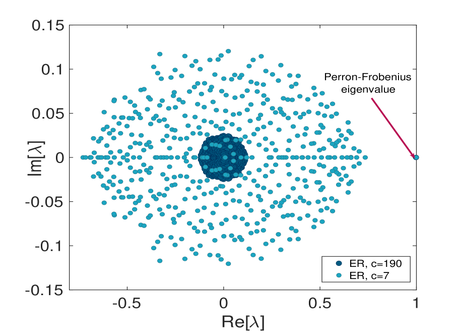
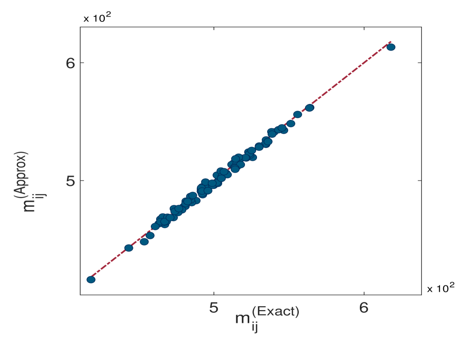
Figure 3: Top: eigenvalues in the complex plane for a typical instance of $T^{(j)}$ for the Erdős-Rényi network described in section 3.2, with edge weights drawn from a uniform $[0,1]$ distribution, and two values of $c$ ($c=190$ (dark blue dots) and $c=7$ (light blue dots)). Clearly the spectral gap is much narrower for the low-$c$ case. Middle: scatter plot of exact results (obtained by matrix inversion, see eq. (3)) vs. our approximate formula in eq. (5). Each point ($100$ in total) refers to a randomly picked $(i,j)$ (source-target) pair, on a randomly generated instance of the graph with $N=500$ and $c=190$. In dashed red, the straight line with slope $=1$, indicating perfect agreement. Bottom: same scatter plot as the middle panel, but with $c=7$ instead.

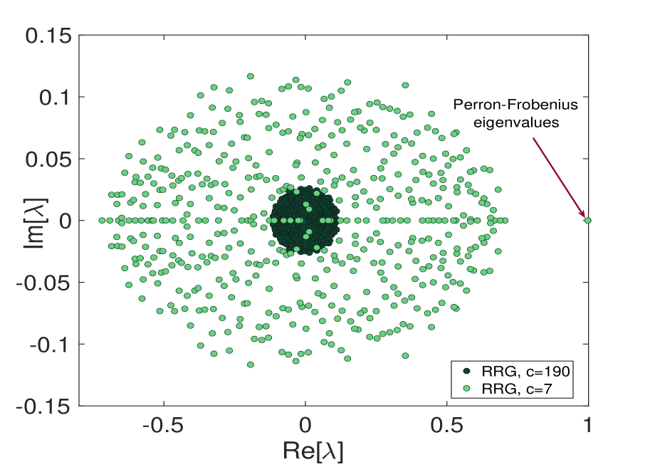
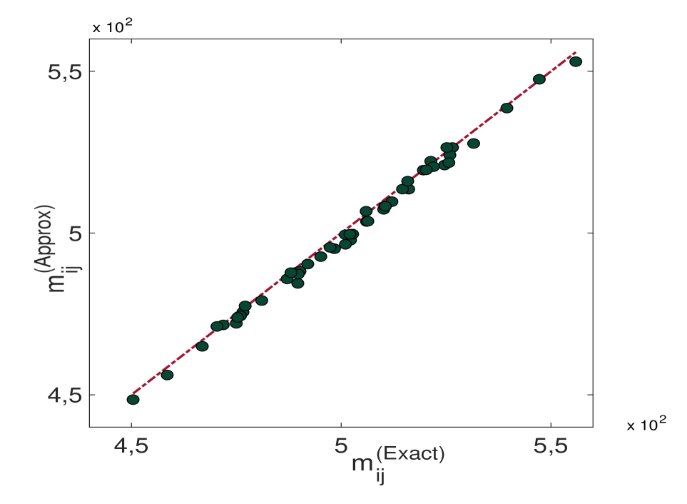
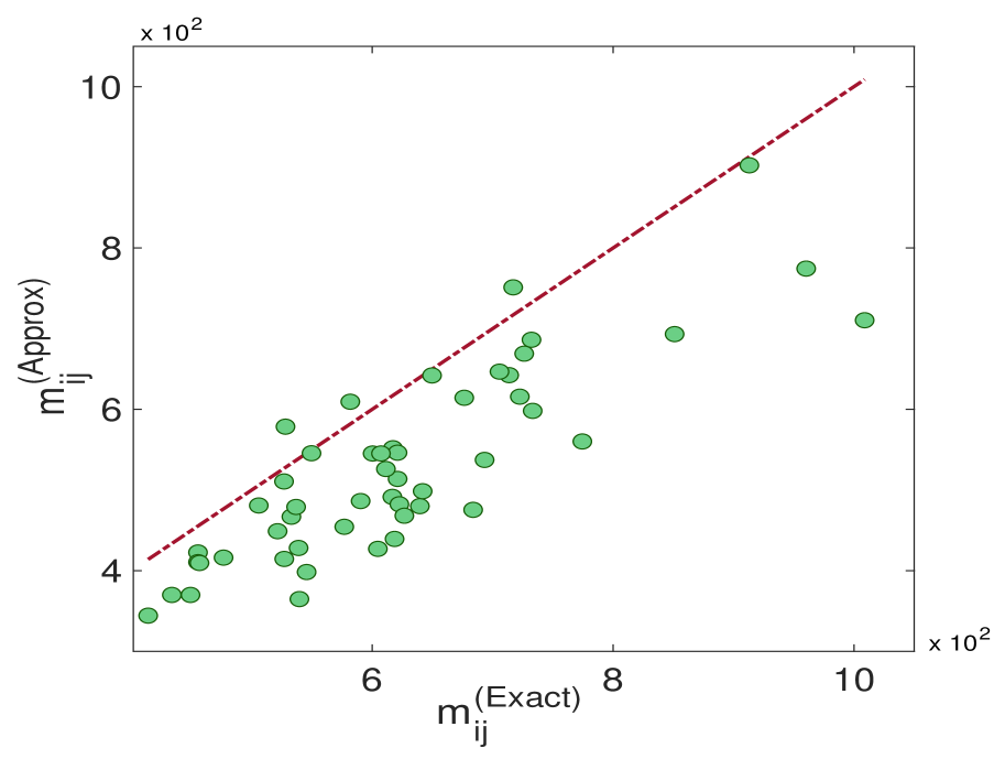
Figure 4: Top: eigenvalues in the complex plane for a typical instance of $T^{(j)}$ for the Random Regular network described in section 3.3 with edge weights drawn from a uniform $[0,1]$ distribution, and two values of $c$ ($c=190$ (dark green dots) and $c=7$ (light green dots)). Clearly the spectral gap is much narrower for the low-$c$ case. Middle: scatter plot of exact results (obtained by matrix inversion, see eq. (3)) vs. our approximate formula in eq. (5). Each point ($50$ in total) refers to a randomly picked $(i,j)$ (source-target) pair, on a randomly generated instance of the graph with $N=500$ and $c=190$. In dashed red, the straight line with slope $=1$, indicating perfect agreement. Bottom: same scatter plot as the middle panel, but with $c=7$ instead.

$c$	Simulations	Exact (3)	Approximate (5)
250	539.11	542.66	542.16
190	486.09	482.57	477.87
100	500.20	502.82	508.09
50	736.03	713.37	692.51
10	499.30	495.04	474.66
4	458.37	464.61	329.45

Table 1: Comparison between simulations, exact, and approximate value for the MFPT on weighted ER networks of different mean connectivity $c$.

$c$	Simulations	Exact (3)	Approximate (5)
250	494.07	492.14	491.08
190	483.79	479.70	478.65
100	474.14	472.14	471.43
50	530.01	524.66	515.85
10	559.02	554.90	453.31
4	990.92	993.19	408.10

Table 2: Comparison between simulations, exact, and approximate value for the MFPT on weighted random regular networks of different connectivity $c$.

4 Conclusions

We have derived the approximate formula (5) for the Mean First Passage Time of a walker between a source node $i$ and a target node $j$ of a (weighted and directed) strongly connected network of $N$ nodes. The formula does not require any (possibly costly and inaccurate) matrix inversion, and takes as input only the local transition weights into the target node. Its accuracy depends on the existence of a “large” spectral gap between the Perron-Frobenius eigenvalue and the blob of all other eigenvalues of the reduced (sub-stochastic) transition matrix $T^{(j)}$ – obtained from the full transition matrix of the walker by erasing the target node’s row and column. We have shown that – for a variety of “not too sparse” networks – this condition is not hard to materialize, and leads to an excellent agreement of our approximate formula with numerical simulations as well as the exact formula (3). While our approach continues to work for (sufficiently dense) heterogeneous networks when the target node is well-connected to the rest of the graph, the intra-row fluctuations around the random matrix assumption $\langle a_{ij}\rangle=z_{i}/N$ may be very significant there and will thus require a more careful treatment.

To our knowledge, our formula (5) is one of the very few, general, and explicit results available in the literature for MFPT on weighted and directed networks (i.e. when the diffusion of the walker is biased by the edge weights), and reduces to known results for the fully connected and dense Erdős-Rényi cases when the diffusion is unbiased.

The formula would be exact if $T^{(j)}$ were a rank-$1$ matrix with $[T^{(j)}]_{k\ell}=(1-T_{kj})/(N-1)$ for all $\ell$ (see eq. (9)). It is also exact to leading order in $N$ as the average value of the MFPT over an ensemble of random matrices with prescribed average $\langle T^{(j)}\rangle$ and sufficiently “narrow” fluctuations: this is the result of the random matrix calculation we first outlined in [36, 37], which is reported here in section 2 for completeness.

Our work leaves a few questions open that would be very interesting to tackle in future studies:

1. How to formally prove the conjecture that a random ensemble satisfying the cumulant decay condition (21) necessarily has a large spectral gap, without assuming Gaussianity?

2. Is it possible to characterize how the accuracy of our formula (5) depends on network observables (e.g. average connectivity and other structural properties of the underlying network), which in turn influence the spectral gap?

3. In [36, 37] we observed that an “improved” formula (22) could be obtained by assuming that not only the row sums of the sub-stochastic matrix $A$ were known, but also the column sums. It would be interesting to see what effect the inclusion of information about the column sums of $T^{(j)}$ might have on the final formula (5).

4. From the random matrix viewpoint, it would be very interesting to consider the model (6) with the hard constraint of positivity (which of course bounds the fluctuations of $\delta A$ and precludes Gaussianity). Alternatively, one could consider a “soft” version of the positivity constraint for a deformed Ginibre ensemble, where one bounds the probability of having negative entries and studies in more details what constraints this poses on the spectrum in the complex plane. The investigation of a “phase transition” whereby the Perron-Frobenius outlier is swallowed by the spectral bulk as the variance of $\delta A_{ij}$ increases is particularly interesting and timely (see [75]).

5. Studying more systematically how the accuracy of the main formula (5) – related to the spectral gap of $T^{(j)}$ – varies with the choice of the target node $j$ on the same instance of a heterogeneous graph is also an interesting question that deserves further investigation (see Appendix B for a preliminary attempt). Along the same lines, also the impact of degree-degree correlations on the accuracy of the formula would be interesting to study in greater detail.

These directions will be the focus of future research.

Appendix A Joint cumulant generating function for Gaussian $\delta h_{ij}$

In this Appendix, we compute explicitly the joint cumulant generating function (20) for the case of i.i.d. Gaussian entries $\delta h_{ij}$ with mean zero and variance $\sigma_{N}^{2}$. We have

$$\varphi\left(\{\theta_{ij}\}\right) =\Big{\langle}\mathrm{e}^{\mathrm{i}\sum_{i,j}^{N}\delta h_{ji}\theta_{ij}}\Big{\rangle}=\prod_{i,j}\int\frac{\mathrm{d}x}{\sqrt{2\pi\sigma_{N}^{2}}}~{}\exp\left[-\frac{x^{2}}{2\sigma_{N}^{2}}+\mathrm{i}x\theta_{ij}\right]$$

$$=\exp\left[-\frac{1}{2}\sigma_{N}^{2}\sum_{i,j}\theta_{ij}\right]\ .$$ (23)

Assuming $\theta_{ij}\sim\mathcal{O}(1)$, the cumulant decay condition (21) requires

$$N^{2}\sigma_{N}^{2}=o(N)\Rightarrow\sigma_{N}=o(1/\sqrt{N})$$ (24)

as stated earlier.

Appendix B The accuracy of (5) and heterogeneous networks: the star graph case

In this Appendix, we test on a simple and exactly solvable case (the star graph with $N$ nodes) the hypothesis that the accuracy of our approximate formula (5) may vary (within the same instance) from node to node, depending on how well connected the target node is to the rest of the network.

The star graph consists of a central node that is connected to all other nodes (leaves), while each leaf is only connected to the central node (has degree $1$). Since the degree of the central node is therefore $N-1$, and our formula (5) is only sensitive to the incoming weights into the target, we may expect some discrepancy in how well (5) works between the the two situations (i) MFPT $m_{i1}$ between a leaf $i$ and the central node (labelled by $1$), and (ii) MFPT $m_{1j}$ between the central node and a leaf $j$. Since the heterogeneity between central node and leaves increases with $N$, we expect that such discrepancy should also get larger for bigger networks.

Considering the standard (unbiased) diffusion for simplicity, the full $N\times N$ transition matrix $T$ reads

$$T=\begin{pmatrix}0&\vline&\begin{matrix}\frac{1}{N-1}&\frac{1}{N-1}&\cdots&\frac{1}{N-1}\\ \end{matrix}\\ \hline\cr\begin{matrix}1\\ 1\\ \vdots\\ 1\end{matrix}&\vline&\mbox{\Large 0}\end{pmatrix}\ .$$

Clearly, $m_{i1}=1$ identically for all $i\geq 2$, which – on top of being obvious given the geometry of the system – emerges from an exact evaluation of Eq. (3), as the reduced transition matrix $T^{(1)}$ is simply the $(N-1)\times(N-1)$ null matrix in this case. For this scenario, our approximate formula (5) provides the same (exact) result, as $T_{i1}=1$, which kills the second fraction in (5).

Conversely, to compute the matrix $(\mathds{1}-T^{(j)})^{-1}$ exactly for $j>1$ – necessary to deal with case (ii) – we need to use the block-matrix inversion formula that yields

$$(\mathds{1}-T^{(j)})^{-1}=\begin{pmatrix}N-1&\vline&\begin{matrix}1&1&1&\cdots&1\\ \end{matrix}\\ \hline\cr\begin{matrix}N-1\\ N-1\\ \vdots\\ N-1\end{matrix}&\vline&\begin{matrix}2&1&1&\cdots&1\\ 1&2&1&\cdots&1\\ \vdots&\vdots&\vdots&\ddots&\vdots\\ 1&1&1&\cdots&2\\ \end{matrix}\end{pmatrix}\ .$$

This gives $m_{1j}=2N-3$ for all $j>1$. In this scenario, though, our approximate formula gives a different result, namely $m_{1j}\approx 1+(N-1)(N-2)$. The two formulae (exact and approximate) yield the same numerical value for low $N$ ($N=2,3$), with the discrepancy growing with $N$. This means that our approximate formula becomes less and less accurate the fewer connections the target node has with the rest of the network. This simple example, therefore, corroborates the intuition that the accuracy of our main formula (5) can vary from node to node within the same instance, depending on how “well-connected” the target node is to the rest of the graph.

References

- [1] D. Aldous, J. A. Fill. Reversible Markov chains and random walks on graphs, available at http://www.stat.berkeley.edu/~aldous/RWG/book.html (2002).
- [2] G. H. Weiss. Random Walks and Random Environments, Volume 1: Random Walks. J. Stat. Phys. 82, 1675–1677 (1996). https://doi.org/10.1007/BF02183400
- [3] S. Redner. A Guide to First-Passage Processes. Cambridge University Press. Cambridge, UK (2001). https://doi.org/10.1017/CBO9780511606014
- [4] D. ben-Avraham, S. Havlin. Diffusion and Reactions in Fractals and Disordered Systems. Cambridge University Press, Cambridge, UK (2000). https://doi.org/10.1017/CBO9780511605826
- [5] L. Lovász. Random walks on graphs: A survey, in: D. Miklós, V. T. Sós, T. Szőnyi (Eds.), Combinatorics, Paul Erdős is Eighty, Volume 1, János Bolyai Math. Soc., Budapest, Hungary, pp. 353–398 (1993).
- [6] R. Burioni, D. Cassi. Random walks on graphs: Ideas, techniques and results. J. Phys. A 38, R45–R78 (2005). https://doi.org/10.1088/0305-4470/38/8/r01
- [7] G. M. Viswanathan, S. V. Buldyrev, S. Havlin, M. G. E. da Luz, E. P. Raposo, H. E. Stanley. Optimizing the success of random searches. Nature 401, 911–914 (1999). https://doi.org/10.1038/44831
- [8] E. A. Codling, M. J. Plank, S. Benhamou. Random walk models in biology. J. R. Soc. Interface 5, 813–834 (2008). https://doi.org/10.1098/rsif.2008.0014
- [9] S. Havlin, D. ben-Avraham. Diffusion in disordered media. Adv. Phys. 36, 695–798 (1987). https://doi.org/10.1080/00018738700101072
- [10] P. G. Doyle, J. L. Snell. Random Walks and Electric Networks. Mathematical Association of America, Washington, DC, USA (1984). arXiv:math/0001057 [math.PR]
- [11] M. A. Porter, G. Bianconi. Editorial: Network analysis and modelling: Special issue of European Journal of Applied Mathematics. Eur. J. Appl. Math. 27, 807–811 (2016). doi:10.1017/S0956792516000334
- [12] S. Boccaletti, V. Latora, Y. Moreno, M. Chavez, D. U. Hwang. Complex networks: Structure and dynamics. Phys. Rep. 424, 175–308 (2006). https://doi.org/10.1016/j.physrep.2005.10.009
- [13] S. H. Strogatz. Exploring complex networks. Nature 410, 268–276 (2001). https://doi.org/10.1038/35065725
- [14] A. Barrat, M. Barthélemy, A. Vespignani. Dynamical Processes on Complex Networks. Cambridge University Press, Cambridge, UK (2008). https://doi.org/10.1017/CBO9780511791383
- [15] E. W. Montroll, G. H. Weiss. Random walks on lattices II. J. Math. Phys. 6 167––181, (1965). https://doi.org/10.1063/1.1704269
- [16] P. Blanchard, D. Volchenkov. Random Walks and Diffusions on Graphs and Databases: An Introduction. Springer, Heidelberg, Germany (2011). doi:10.1007/978-3-642-19592-1
- [17] Z. Zhang, T. Shan, G. Chen. Random walks on weighted networks. Phys. Rev. E 87, 012112 (2013). doi:10.1103/PhysRevE.87.012112
- [18] S. J. Yang. Exploring complex networks by walking on them. Phys. Rev. E 71, 016107 (2005). doi:10.1103/PhysRevE.71.016107
- [19] L. da Fontoura Costa, G. Travieso. Exploring complex networks through random walks. Phys. Rev. E 75, 016102 (2007). doi:10.1103/PhysRevE.75.016102
- [20] A. Baronchelli, M. Catanzaro, R. Pastor-Satorras. Random walks on complex trees. Phys. Rev. E 78, 011114 (2008). doi:10.1103/PhysRevE.78.011114
- [21] N. Masuda, M. A. Porter, R. Lambiotte. Random walks and diffusion on networks. Physics Reports 716–717, 1-58 (2017). https://doi.org/10.1016/j.physrep.2017.07.007
- [22] T. S. Evans, J. P. Saramäki. Scale-free networks from self-organization. Phys. Rev. E 72, 026138 (2005). doi:10.1103/PhysRevE.72.026138
- [23] N. Ikeda. Network formation determined by the diffusion process of random walkers. J. Phys. A: Math. Theor. 41, 235005 (2008). https://doi.org/10.1088/1751-8113/41/23/235005
- [24] F. Caravelli, A. Hamma, M. Di Ventra. Scale-free networks as an epiphenomenon of memory. EPL 109, 28006 (2015). doi:10.1209/0295-5075/109/28006
- [25] N. F. Polizzi, M. J. Therien, D. N. Beratan. Mean First‐Passage Times in Biology. Israel Journal of Chemistry, 56(9-10), pp.816-824 (2016). doi:10.1002/ijch.201600040
- [26] R. Belousov, M. N. Qaisrani, A. Hassanali, É. Roldán. First-passage fingerprints of water diffusion near glutamine surfaces. Soft Matter 16, 9202 (2020). https://doi.org/10.1039/D0SM00541J
- [27] R. Chicheportiche, J.-P. Bouchaud. Some applications of first-passage ideas to finance. In “First-passage Phenomena And Their Applications” edited by R. Metzler, G. Oshanin, S. Redner (pp. 447-476) (2014). https://doi.org/10.1142/9104
- [28] H. McKenzie, M. Lewis, E. Merrill. First passage time analysis of animal movement and insights into the functional response. Bull. Math. Biol. 71:107–129 (2009). https://doi.org/10.1007/s11538-008-9354-x
- [29] A. Kells, V. Koskin, E. Rosta, A. Annibale. Correlation functions, mean first passage times, and the Kemeny constant. J. Chem. Phys. 152, 104108 (2020). doi:10.1063/1.5143504
- [30] O. Bénichou, R. Voituriez. From first-passage times of random walks in confinement to geometry-controlled kinetics. Phys. Rep. 539, 225–284 (2014). https://doi.org/10.1016/j.physrep.2014.02.003
- [31] S. White, P. Smyth. Algorithms for estimating relative importance in networks. In “Proceedings of the ninth ACM SIGKDD international conference on Knowledge discovery and data mining”, ser. KDD ’03. New York, NY, USA: ACM, pp. 266–275 (2003). https://doi.org/10.1145/956750.956782
- [32] S. Vigna. Spectral Ranking. Network Science 4(4), 433-445 (2016). doi:10.1017/nws.2016.21
- [33] Z. Q. Lee, W. Hsu, M. Lin. Efficient algorithm for ranking of nodes’ importance in information dissemination. In “Proceedings of the 2014 IEEE/ACM International Conference on Advances in Social Networks Analysis and Mining” (ASONAM ’14). IEEE Press, 89–92 (2014). doi: 10.1109/ASONAM.2014.6921565
- [34] A. Bassolas, V. Nicosia. First-passage times to quantify and compare structural correlations and heterogeneity in complex systems. Commun. Phys. 4, 76 (2021). https://doi.org/10.1038/s42005-021-00580-w
- [35] Z. Zheng, G. Xiao, G. Wang, G. Zhang, K. Jiang. Mean first passage time of preferential random walks on complex networks with applications. Mathematical Problems in Engineering vol. 2017, Article ID 8217361 (2017). https://doi.org/10.1155/2017/8217361
- [36] S. Bartolucci, F. Caccioli, F. Caravelli, P. Vivo. Universal rankings in complex input-output organizations. Preprint arXiv:2009.06307v3 (2020).
- [37] S. Bartolucci, F. Caccioli, F. Caravelli, P. Vivo. Inversion-free Leontief inverse: statistical regularities in input-output analysis from partial information. Preprint arXiv:2009.06350v3 (2020).
- [38] J. G. Kemeny, J. L. Snell. Finite Markov Chains (Second Ed.). Springer-Verlag, New York, NY, USA (1976).
- [39] A. Papoulis, S. U. Pillai. Probability, Random Variables, and Stochastic Processes. 4th Edition, McGraw-Hill, New York, NY, USA (2002).
- [40] W. J. Stewart. Introduction to the Numerical Solution of Markov Chains. Princeton University Press, Princeton, NJ, USA (1994).
- [41] Y. Lin, Z. Zhang. Random walks in weighted networks with a perfect trap: An application of Laplacian spectra. Phys. Rev. E 87, 062140 (2013). doi:10.1103/PhysRevE.87.062140
- [42] P. S. Dwyer, F. V. Waugh. On Errors in Matrix Inversion. Journal of the American Statistical Association 48(262), 289-319 (1953). https://doi.org/10.2307/2281289
- [43] J. D. Noh, H. Rieger. Random walks on complex networks. Phys. Rev. Lett. 92, 118701 (2004). doi:10.1103/PhysRevLett.92.118701
- [44] A. Fronczak, P. Fronczak. Biased random walks in complex networks: The role of local navigation rules. Phys. Rev. E 80, 016107 (2009). https://doi.org/10.1103/PhysRevE.80.016107
- [45] A. Baronchelli, R. Pastor-Satorras. Mean-field diffusive dynamics on weighted networks. Phys. Rev. E 82, 011111 (2010). doi:10.1103/PhysRevE.82.011111
- [46] A. Kittas, S. Carmi, S. Havlin, P. Argyrakis. Trapping in complex networks. EPL 84, 40008 (2008). https://doi.org/10.1209/0295-5075/84/40008
- [47] N. Perra, A. Baronchelli, D. Mocanu, B. Gonçalves, R. Pastor-Satorras, A. Vespignani. Random walks and search in time-varying networks. Phys. Rev. Lett. 109, 238701 (2012). https://doi.org/10.1103/PhysRevLett.109.238701
- [48] M. Starnini, A. Baronchelli, A. Barrat, R. Pastor-Satorras. Random walks on temporal networks. Phys. Rev. E 85, 056115 (2012). https://doi.org/10.1103/PhysRevE.85.056115
- [49] A. Baronchelli, V. Loreto. Ring structures and mean first passage time in networks. Phys. Rev. E 73, 026103 (2006). doi:10.1103/PhysRevE.73.026103
- [50] O. C. Martin, P. Šulc. Return probabilities and hitting times of random walks on sparse Erdős-Rényi graphs. Phys. Rev. E 81, 031111 (2010). https://doi.org/10.1103/PhysRevE.81.031111
- [51] S. Hwang, D. S. Lee, B. Kahng. Origin of the hub spectral dimension in scale-free networks. Phys. Rev. E 87, 022816 (2013). doi:10.1103/PhysRevE.87.022816
- [52] L. K. Gallos, C. Song, S. Havlin, H. A. Makse. Scaling theory of transport in complex biological networks. Proc. Natl. Acad. Sci. USA 104, 7746–7751 (2007). https://doi.org/10.1073/pnas.0700250104
- [53] E. Agliari. Exact mean first-passage time on the T-graph. Phys. Rev. E 77, 011128 (2008). doi:10.1103/PhysRevE.77.011128
- [54] E. Agliari, R. Burioni. Random walks on deterministic scale-free networks: Exact results. Phys. Rev. E 80, 031125 (2009). doi:10.1103/PhysRevE.80.031125
- [55] R. B. Bapat. On the first passage time of a simple random walk on a tree. Statistics Probability Letters 81(10), 1552 (2011). https://doi.org/10.1016/j.spl.2011.05.017
- [56] S. Hwang, D. S. Lee, B. Kahng. First passage time for random walks in heterogeneous networks. Phys. Rev. Lett. 109, 088701 (2012). doi:10.1103/PhysRevLett.109.088701
- [57] Z. Zhang, Y. Qi, S. Zhou, S. Gao, J. Guan. Explicit determination of mean first-passage time for random walks on deterministic uniform recursive trees. Phys. Rev. E 81, 016114 (2010). doi:10.1103/PhysRevE.81.016114
- [58] N. Masuda, N. Konno. Return times of random walk on generalized random graphs. Phys. Rev. E 69, 066113 (2004). doi:10.1103/PhysRevE.69.066113
- [59] H. W. Lau, K. Y. Szeto. Asymptotic analysis of first passage time in complex networks. EPL 90, 40005 (2010). doi:10.1209/0295-5075/90/40005
- [60] S. Condamin, O. Bénichou, V. Tejedor, R. Voituriez, J. Klafter. First-passage times in complex scale-invariant media. Nature 450, 77–80 (2007). https://doi.org/10.1038/nature06201
- [61] I. Tishby, O. Biham, E. Katzav. The distribution of first hitting times of random walks on directed Erdős-Rényi networks. J. Stat. Mech. 043402 (2017). doi:10.1088/1742-5468/aa657e
- [62] V. Tejedor, O. Bénichou, R. Voituriez. Global mean first-passage times of random walks on complex networks. Phys. Rev. E 80, 065104(R) (2009). doi:10.1103/PhysRevE.80.065104
- [63] D. Cvetković, P. Rowlinson, S. Simić. An Introduction to the Theory of Graph Spectra. Cambridge University Press, Cambridge, UK (2010). https://doi.org/10.1017/CBO9780511801518
- [64] P. Van Mieghem. Graph Spectra for Complex Networks. Cambridge University Press, Cambridge, UK (2011). https://doi.org/10.1017/CBO9780511921681
- [65] V. A. R. Susca, P. Vivo, R. Kühn. Second largest eigenpair statistics for sparse graphs. Journal of Physics A: Mathematical and Theoretical 54(1), 015004 (2020). doi:10.1088/1751-8121/abcbad
- [66] V. Sood, S. Redner, D. ben-Avraham. First-passage properties of the Erdős-Renyi random graph. J. Phys. A 38, 109–123 (2005). doi:10.1088/0305-4470/38/1/007
- [67] M. Löwe, F. Torres. On hitting times for a simple random walk on dense Erdös–Rényi random graphs. Stat. Prob. Lett. 89, 81–88 (2014). https://doi.org/10.1016/j.spl.2014.02.017
- [68] P. Azimzadeh. A fast and stable test to check if a weakly diagonally dominant matrix is a nonsingular M-matrix. Math. Comp. 88, 783-800 (2019). doi:10.1090/mcom/3347
- [69] J. Sherman, W. J. Morrison. Adjustment of an Inverse Matrix Corresponding to a Change in One Element of a Given Matrix. Annals of Mathematical Statistics 21 (1), 124-127 (1950). doi: 10.1214/aoms/1177729893
- [70] J. Ginibre. Statistical ensembles of complex, quaternion, and real matrices. J. Math. Phys. 6, 440–449 (1965). https://doi.org/10.1063/1.1704292
- [71] F. Benaych-Georges, J. Rochet. Outliers in the Single Ring Theorem. Probab. Theory Relat. Fields 165, 313–363 (2016). https://doi.org/10.1007/s00440-015-0632-x
- [72] T. Tao. Outliers in the spectrum of i.i.d. matrices with bounded rank perturbations. Probab. Theory Related Fields 155, 231–263 (2013). https://doi.org/10.1007/s00440-011-0397-9
- [73] S. O’Rourke, D. Renfrew. Low rank perturbations of large elliptic random matrices. Electron. J. Probab. 19, n. 43 (2014). doi: 10.1214/EJP.v19-3057
- [74] C. Bordenave, M. Capitaine. Outlier eigenvalues for deformed i.i.d. random matrices. Communications on Pure and Applied Mathematics 69(11), 2131-2194 (2016). https://doi.org/10.1002/cpa.21629
- [75] F. Mosam, D. Vidaurre, E. De Giuli. Breakdown of random matrix universality in Markov models. Preprint arXiv: arXiv:2105.04393 (2021).
- [76] F. L. Metz, I. Neri, D. Bollé. Localization transition in symmetric random matrices. Phys. Rev. E 82, 031135 (2010). doi:10.1103/PhysRevE.82.031135
- [77] M. Mézard, G. Parisi, M. A. Virasoro. Spin Glass Theory and Beyond. World Scientific (1987). https://doi.org/10.1142/0271
- [78] J. Bun, R. Allez, J. Bouchaud, M. Potters. Rotational Invariant Estimator for General Noisy Matrices. IEEE Transactions on Information Theory 62(12), 7475-7490 (2016). doi:10.1109/TIT.2016.2616132
- [79] J. Kurchan. Supersymmetry, replica and dynamic treatments of disordered systems: a parallel presentation. Markov Processes and Related Fields. Polymath 9(2), 243-260 (2003).
- [80] J. H. Kim, V. H. Vu. Generating Random Regular Graphs. Combinatorica 26, 683–708 (2006). https://doi.org/10.1007/s00493-006-0037-7