Towards real time assessment of earthfill dams via Model Order Reduction

Abstract

The use of Internet of Things (IoT) technologies is becoming a preferred solution for the assessment of tailings dams’ safety. Real-time sensor monitoring proves to be a key tool for reducing the risk related to these ever-evolving earth-fill structures, that exhibit a high rate of sudden and hazardous failures.

In order to optimally exploit real-time embankment monitoring, one major hindrance has to be overcome: the creation of a supporting numerical model for stability analysis, with rapid-enough response to perform data assimilation in real time. A model should be built, such that its response can be obtained faster than the physical evolution of the analyzed phenomenon. In this work, Reduced Order Modelling (ROM) is used to boost computational efficiency in solving the coupled hydro-mechanical system of equations governing the problem.

The Reduced Basis method is applied to the coupled hydro-mechanical equations that govern the groundwater flow, that are made non-linear as a result of considering an unsaturated soil. The resulting model’s performance is assessed by solving a 2D and a 3D problem relevant to tailings dams’ safety. The ROM technique achieves a speedup of 3 to 15 times with respect to the full-order model (FOM) while maintaining high levels of accuracy.

1 Introduction

Tailings is a common by-product of the process of extracting valuable minerals and metals from mined ore. They usually take the form of a liquid slurry made of fine mineral particles, created as mined ore is crushed, ground and processed. The volume of tailings is normally far in excess of the liberated resource and the tailings often contain potentially hazardous contaminants. It is usual practice for tailings to be stored in isolated impoundments under water and behind dams (Kossoff et al., 2014).

Tailings dams are usually constructed by readily available local materials and they are often built of, and/or on tailings material (Saad and Mitri, 2011). Tailings grain size is highly variable and dependent on the parent rock and the method of extraction. They tend however to be largely gravel-free and clay-free, with sand being more common than silt (Kossoff et al., 2014). Their chemical composition depends on the mineralogy of the ore body, the degree of weathering during storage and the extraction process. Silica, Fe and oxygen display an almost universal presence and seem to be the most abundant elements in tailings (Kossoff et al., 2014). Tailings material is pumped from the mill to the impoundment and is often size differentiated during deposition. The coarser and more porous material settles close to the discharge point, near the embankment, and may be used to extend the structure itself, while the finer fraction (slimes) is carried further away forming an impermeable barrier. This size-differentiated dispersal contributes to the integrity of the dam (Kossoff et al., 2014).

Rather than constructed at once, tailings dams are gradually raised, as the mining activity results to larger capacity demands for the storing reservoir. Three different methods are used for embankment level raise, namely the upstream, downstream, and centerline method, as illustrated in Figure 1. The brown-colored part in the Figure represents the part of the structure that has to be constructed of coarse and compacted material, and therefore the most expensive part to be built. The upstream method, requiring the smallest volume of processed fill material, and therefore being the most cost effective, is most widely chosen (Lyu et al., 2019), but it is associated to many major failures. In upstream dams, the additional layers of structure are placed on top of tailings depositions, therefore the construction’s safety depends on the integrity of tailings for stability (Davies and Martin, 2002). This type of dam requires greater ongoing scrutiny (Martin and McRoberts, 1999).

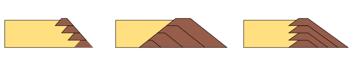
Figure 1: Tailings dam construction method: conceptual illustration. Left to right: Upstream, Downstream, Centreline level raise. Yellow color: Tailings. Brown color: Fill material.

Impoundment failure can be categorized into four basic mechanisms. These main mechanisms are, overtopping, often occurring in inactive structures after a flooding event; localized failure, caused by the presence of a shear band; piping, caused by internal erosion due to seepage; and diffuse failure, triggered by liquefaction of loose tailings material (Hamade, 2013). The common factors in most cases are the importance of the stress and seepage fields on the dam. The seepage field might directly induce instability by erosion, or cause the pore pressure to rise, leading to a reduction of effective stress and shear strength.

Slope instability -that corresponds to the second failure mechanism, local failure- is one of the most common failure modes (Morton, 2021). In upstream tailings dams, the risk of instability of the downstream slope should be particularly investigated during design and monitoring. Stability of upstream dams might depend on the stability of the tailings depositions upstream, that support the overlying layers of the embankment. In case the tailings deposited have a high water content, a fast loading rate that allows no time for consolidation may lead to excess pore pressure and loss of resistance to shear failure. The new layers of structure do not provide a stabilizing force to the downstream slope, as is the case with centerline and downstream raising methods. The timescales of loading, i.e. raising the dam level, and of consolidation of the underlying material, are governing the hydromechanical response of the system.

Obviously, the stability problem in tailings dams should be treated as a hydro-mechanical problem, as it is the excess of pore pressure that causes the loss of cohesive properties of the material and consequently its local failure. High pore pressures, and high hydraulic gradients in the case of erosive failures (piping), are omnipresent elements in tailings dams failures. Pore pressure monitoring is therefore crucial in the case of tailings dams.

Tailings dams’ safety management involves regular sensing and collection of data describing quantities such as pore pressures and deformations (Clarkson et al., 2020). The assessment, however, of such large volumes of data is not always straightforward (Knutsson et al., 2016),(Hui et al., 2018). A common approach is to assess data in terms of trends over time. Expected behaviors are based on previous trends (Knutsson et al., 2016), (Vanden Berghe et al., 2011). This is an appropriate method for monitoring sudden changes that indicate trouble. However, it is not always an appropriate option for non-static structures like tailings dam. During periods when the dam crest level is raised, these structures undergo significant changes. Nonetheless, the induced pore pressures and deformations must remain in the serviceability range.

Monitoring instrumentation and data collection are useful only if they are used in combination with appropriate numerical models capable of describing the hydro-mechanical coupling that governs the problem (Szostak et al., 2003). These models can contribute to identifying undesirable behaviors, thus making sense of the collected data, and establishing appropriate alarm functions.

A common challenge in developing realistic models is related to highly uncertain parameters, mainly representing material properties (Heshmati R. et al., 2020). The hydraulic and mechanical properties of the structural and stored materials are often unknown and may vary over time (Villavicencio et al., 2011). To treat such problems efficiently, data assimilation may prove useful. In this context, field measurements are used for back-analyses in order to identify realistic values for the properties used in the model. Data assimilation, implies the solution of an inverse problem, that is, a problem that examines multiple solutions for different values of the parameters, and identifies the most realistic parametric values by driving the model output as close to the reality.

The use of such methods in a real-time framework presupposes the existence of a numerical model, able to provide responses to many-query problems, faster than the evolution of the physical phenomenon that is analyzed. Reduced Order Models (ROM) prove to be a suitable solution for guaranteeing accurate and fast queries. Model Order Reduction is a set of techniques that aim to enhance a model’s computational efficiency by decreasing its dimensionality, that is, the number of degrees of freedom that correspond to the discretized problem.

Data assimilation and inverse problem solving motivate this work, but are not treated in the present paper. This work focuses on implementing Model Order Reduction on the fully coupled hydro-mechanical equations that govern water flow through unsaturated soil.

There have been several model reduction methodologies applied to the simulation of porous media flow, such as data-driven models (Bao et al., 2019) (Ghommem et al., 2016), Proper Orthogonal Decomposition (POD) based methods (Ghommem et al., 2016) (van Doren et al., 2006) (Larion et al., 2020) (Badia et al., 2009), as well as POD paired with DEIM (Discrete Empirical Interpolation Method) where the non-linear terms are approximated by some form of interpolation, ensuring a large reduction of computational cost (Gildin et al., 2013) (Esmaeili et al., 2020). The work in all the papers mentioned above is motivated by reservoir and petroleum engineering and often refers to multiphase fluid flow. In the aforementioned papers, POD-based reduction is applied to the hydraulic problem alone, and does not concern the hydro-mechanically coupled problem (Ghommem et al., 2016) (Gildin et al., 2013) (van Doren et al., 2006) (Vermeulen et al., 2004).

The original contribution of this work, lies in the implementation of POD-based reduction for the coupled non-linear problem, considering partial saturation of the porous medium. Coupling of the two equations that govern the mechanical and hydraulic part of the problem, yields a non-linear transient system of equations, that is discretized using the Finite Element Method. Non-linearities are introduced in order to describe partially saturated states for the soil. Partial saturation must be considered in the study of earthdams, as it is a common occurrence in these structures that the water table is located below the dam crest, and therefore only part of the material is saturated. Solving the discretized system of equations, one can obtain the full-order or high fidelity approximation of the solution to the PDEs. The Reduced Basis method (Florentin and Díez, 2012) (Maday and Rønquist, 2002) (Maday and Ronquist, 2004) (Rozza et al., 2007) represents an instance of model order reduction techniques in which the parametric dependence of the PDE solution is explored by solving the high-fidelity problem a number of times. The resulting set of solutions is explored in a POD framework, in order to find a set of elements, hopefully fewer in number than the dimension of the full-order problem, the linear combination of which can provide a satisfactory approximation of the high-fidelity solution.

To adapt this technique problems in partially saturated soils, the paper is structured as follows. Sections 2 to 3 contain a detailed description of the methodologies used for developing the forward FE model and the low-order approximation model using RB. In Section 4 some details on the implementation tool are given. In Section 5 the accuracy and computational efficiency achieved with ROM are demonstrated solving a problem related to the construction of tailings dams. The results are discussed and an outline of future work that could add value to the present work is given in section 6.

2 Constitutive relations and governing equations

In this Section, the equations that govern the hydro-mechanically coupled problem of groundwater flow through an unsaturated soil are presented. The equations written here describe various geomechanical problems that feature water flow through unsaturated porous media, and the methodologies developed in this work can be used to solve these problems.

2.1 Conservation of linear momentum

The equation of mechanical equilibrium reads

$$\boldsymbol{\nabla}^{\intercal}\boldsymbol{\sigma}+\mathbf{b}=\mathbf{0},$$ (1)

where $\boldsymbol{\sigma}$ is the total stress tensor, and $\mathbf{b}$ is the vector of body forces

$$\rm{\mathbf{b}=\rho(p)\mathbf{g}},$$ (2)

where $\mathbf{g}=[0,0,-g]^{\intercal}$ is the gravity acceleration vector in a 3D setting, and $\rho$ is the density of the multiphase medium, comprised of soil particles and water, evaluated as a function of pore water pressure $\rm{p}$, and related to the density of soil particles and water ($\rm{\rho_{s},\rho_{w}}$) according to the relation

$$\rm{\rho(p)=(1-\eta)\rho_{s}+\eta S_{e}(p)\rho_{w}=(1-\eta)\rho_{s}+\Theta(p)\rho_{w}}$$ (3)

where $\eta$ denotes the soil porosity. The volume water content (VWC) $\rm{\Theta(p)}$ and effective degree of saturation $\rm{S_{e}(p)}$ are evaluated according to a hydraulic model detailed in Section 2.3

In this work the air pressure is considered equal to the atmospheric pressure, as commonly assumed in geotechnics. The constitutive stress is defined as

$$\boldsymbol{\sigma}^{\prime}=\boldsymbol{\sigma}-\rm{S_{e}(p)}\mathrm{p}\mathbf{I}.$$ (4)

where $\boldsymbol{\sigma^{\prime}}$ is the tensor of effective stresses, $\mathbf{I}$ the identity matrix and $\rm{S_{e}}$ the effective degree of saturation (Nuth and Laloui, 2008), or dimensionless water content, which is one of the factors among many (Nuth and Laloui, 2008) that have been proposed in order to weight the contributions of the two phases, soil and water, to the total stress. The effective degree of saturation is suction dependent and will be estimated as explained in Section 2.3.

Introducing the concept of effective stress $\boldsymbol{\sigma}^{\prime}$ as defined in equation (4) in the mechanical equilibrium (1), yields,

$$\rm{\boldsymbol{\nabla}^{\intercal}\left(\boldsymbol{\sigma}^{\prime}+S_{e}(p)\rm{p}\mathbf{I}\right)+\mathbf{b}=\mathbf{0}}$$ (5)

Linear elasticity is assumed for the soil skeleton’s response. In that framework, the constitutive stress-strain relation reads

$$\boldsymbol{\sigma}^{\prime}=\lambda tr\boldsymbol{\varepsilon}(\mathbf{u})\mathbf{I}+2\mu\boldsymbol{\varepsilon}(\mathbf{u})$$ (6)

where $\mathbf{u}$ is the displacement vector, $\boldsymbol{\varepsilon}$ denotes the infinitesimal strain tensor, calculated as $\boldsymbol{\varepsilon}(\mathbf{u})=\frac{\boldsymbol{\nabla}\mathbf{u}+\boldsymbol{\nabla}^{\intercal}\mathbf{u}}{2}$ , and $\lambda$ and $\mu$ are the Lamé elastic moduli. The usual parameters defining the elastic mechanical material characteristics are the Young’s modulus $\rm{E}$ and Poisson’s ratio $\rm{\nu}$, but the constitutive models are often written in terms of Lamé coefficients. For isotropic 3-dimensional materials and for plane strain conditions in 2 dimensions, the relations among these parameters are,

$$\rm{\mu}=\rm{\frac{E}{2(1+\nu)}},\quad\rm{\lambda}=\rm{\frac{E\nu}{(1+\nu)(1-2\nu)}}.$$ (7)

Introducing the stress-strain relation, the mechanical equilibrium can be written in the form:

$$\rm{\boldsymbol{\nabla}^{\intercal}\left(\lambda tr\boldsymbol{\varepsilon}(\mathbf{u})\mathbf{I}+2\mu\boldsymbol{\varepsilon}(\mathbf{u})+S_{e}(p)\rm{p}\mathbf{I}\right)+\rho(p)\mathbf{g}=\mathbf{0}}$$ (8)

The governing equation (1) is accompanied by boundary conditions to formulate a boundary value problem. For the mechanical part of the problem, Dirichlet conditions are used to impose constraints in displacement and Neumann conditions to apply a load.

Let $\rm{\Gamma_{D}^{u}}$, $\rm{\Gamma_{N}^{u}}$ and be two partitions of the boundary $\rm{\partial\Omega}$ of the domain $\rm{\Omega}$ on which Dirichlet and Neumann boundary conditions are applied respectively. The boundary conditions are:

$$\rm{\boldsymbol{\mathbf{u}}} =\hat{\mathbf{u}}\quad\text{on}\ \rm{\Gamma_{D}^{u}}$$ (9)

$$\rm{\boldsymbol{\sigma}\cdot\mathbf{n}} =\rm{\hat{\mathbf{t}}}\quad\text{on}\ \Gamma_{N}^{u}$$ (10)

where $\rm{\mathbf{n}}$ is the outward pointing unit normal vector and $\rm{\hat{\mathbf{t}}}$ is the surface traction force.

2.2 Water mass conservation

Considering the mass balance of pore fluids leads to the continuity equation for flow, stating that the water outflow from a representative elementary volume is equal to the changes in mass concentration. Neglecting the deformations of solid particles due to effective stress and pore pressure, and the density gradients of water, introducing the Darcian definition for fluid velocity stated in equation (12), the strong form of the continuity equation reads

$$\rm{\boldsymbol{\nabla}^{\intercal}\big{[} \frac{k(p)}{\gamma_{w}}(\boldsymbol{\nabla}\mathrm{p}+\mathbf{b}_{w}) \big{]} +\bigg{(}C(p)-\frac{\Theta(p)}{K_{w}}\bigg{)}\dot{\mathrm{p}}=\Theta(p)\boldsymbol{\nabla}\cdot\dot{\mathbf{u}}},$$ (11)

where $\rm{\mathbf{b}_{w}=\rho_{w}\mathbf{g}}$ are the body water forces and $\rm{K_{w}}$ is the water bulk modulus. The hydraulic conductivity $\rm{k(p)}$, specific moisture capacity $\rm{C(p)}$, and volumetric water content (VWC) $\rm{\Theta(p)}$ are estimated using the soil water retention relations that are presented in Section 2.3.

The governing equation describing water flow is transient, with two time dependent terms. One contains the time derivative of pore pressure $\dot{\mathrm{p}}$, and the other, a coupling term which accounts for the change in porosity due to the overall compression of the soil structure, and contains the time derivative of the volumetric strain $\dot{\mathbf{u}}$ of the medium. The specific discharge, or fluid velocity $\mathbf{q}$ can be related to the pore water pressure gradient $\rm{\boldsymbol{\nabla}p}$ according to Darcy’s law, which for an isotropic material takes the form

$$\rm{\mathbf{q}=-\frac{k(p)}{\gamma_{w}}(\boldsymbol{\nabla}\mathrm{p}+\mathbf{b}_{w}}),$$ (12)

where $\rm{k}$ is the hydraulic conductivity of the multiphase medium measured in (m/s), $\rm{\gamma_{w}}$ is the specific weight of water and $\rm{\mathbf{b}_{w}}$ is the vector of fluid body forces.

Typical boundary conditions that arise in the case of earthfill dams may be either of Dirichlet, Newmann or Robin type. For the flow equation, Dirichlet conditions may be used to prescribe a known hydraulic head, Neumann conditions for a known outflow, inflow or a hydraulically closed (impervious) boundary.

A particular case arises in the description of a seepage face, which occurs when a water table touches an open downstream boundary (Pinyol et al., 2008) (Gerard et al., 2009). The length of the seepage surface is pressure-dependent (Alonso et al., 2005), and can be prescribed as a non-linear Robin condition.

Let $\rm{\Gamma_{D}^{p}}$, $\rm{\Gamma_{N}^{p}}$ and $\rm{\Gamma_{R}^{p}}$ be three partitions of the boundary $\rm{\partial\Omega}$ of the domain $\rm{\Omega}$ on which Dirichlet, Neumann and Robin boundary conditions are applied respectively. The boundary conditions are:

$$\rm{p} =\hat{\rm{p}}\quad\text{on}\ \rm{\Gamma_{D}^{p}}$$ (13)

$$\rm{\mathbf{q}\cdot\mathbf{n}} =\rm{\hat{q}}\quad\text{on}\ \Gamma_{N}^{p}$$ (14)

$$\rm{\mathbf{q}\cdot\mathbf{n}} =\rm{\langle\beta p\rangle}\quad\text{on}\ \Gamma_{R}^{p}$$ (15)

where $\rm{\mathbf{n}}$ is the outward pointing normal vector and $\rm{\hat{q}}$ is the fluid flux on the boundary. Equation (15) refers to the seepage condition, where the non-linear function of $\rm{p}$ that is denoted with angular brackets prescribes a flux that is equal to $\rm{\beta p}$, when $\rm{p}>0$ and vanishes for negative pressure. The coefficient $\beta$ depends on the hydraulic conductivity and geometry of the domain and defines the water runoff on a boundary in seepage conditions. This is a non-linear Robin type condition.

2.3 Soil water characteristics

The most commonly used hydraulic model for the water content - pore water pressure relation in unsaturated soils is the one proposed by Van Genuchten (van Genuchten, 1980). The effective saturation $\rm{S_{e}}$ -or dimensionless water content- is given by

$$\rm{S_{e}(p)}=\left\{ \begin{array}[]{ll}\rm{\frac{1}{[1+(\alpha|\frac{p}{\gamma_{w}}|)^{\frac{1}{1-m}}]^{m}}}&\rm{p<0}\\ \rm{1}&\rm{p\geq 0}\\ \end{array}\right.$$ (16)

where $\rm{\alpha}$ is a parameter related to the air entry value of the soil and $\rm{m}$ is a curve fitting parameter. The upper branch of this equation describes a sigmoid curve which is called a water-retention curve. The VWC is then given by

$$\rm{\Theta(p)=S_{e}(p)(\Theta_{s}-\Theta_{r})+\Theta_{r}}$$ (17)

where $\rm{\Theta_{s},\Theta_{r}}$ are soil characteristics: the VWC for fully saturated conditions, and the residual VWC. Differentiation of equation (17) with respect to pore water pressure gives

$$\rm{C(p)=\frac{\partial\Theta(p)}{\partial p}=\frac{-\alpha m(\Theta_{s}-\Theta_{r})}{1-m}S_{e}(p)^{1/m}(1-S_{e}(p)^{1/m})^{m}}.$$ (18)

The relation between the hydraulic conductivity of the soil-water system and the pore water pressure as proposed by van Genuchten (van Genuchten, 1980) reads,

$$\rm{k(p)=k_{s}\sqrt{S_{e}(p)}\big{[}1-\big{(}1-S_{e}(p)^{1/m}\big{)}^{m}\big{]}^{2}}$$ (19)

where $\rm{k_{s}}$ is the hydraulic conductivity for saturated conditions.

3 Model reduction methodology

3.1 Finite Element Method for hydro-mechanical groundwater flow problems in unsaturated conditions

Multiplying equation (8) with a vector test function $\mathbf{v}$, integrating over the domain $\Omega$, and applying the Green-Gauss theorem, the variational form is obtained:

$$\int_{\Omega}\boldsymbol{\sigma}^{\prime}\mathrel{\mathop{\mathchar 58\relax}}\boldsymbol{\varepsilon}{(\mathbf{v})}\rm{dx}-\int_{\Omega}S_{e}\rm{p}\mathbf{I}\mathrel{\mathop{\mathchar 58\relax}}\boldsymbol{\varepsilon}{(\mathbf{v})}\rm{dx}=\int_{\Omega}\mathbf{b}\mathbf{v}\rm{dx}+\int_{\Gamma_{N}^{\mathbf{u}}}(\boldsymbol{\sigma}\cdot\mathbf{n})\mathbf{v}\rm{ds}$$ (20)

The equation is discretized applying the Galerkin approach. The discretized equation reads

$$\mathbf{K}\mathbf{U}-\mathbf{Q}\mathbf{P}=\mathbf{f_{u}}$$ (21)

where,

$$\mathbf{K} =\rm{\int_{\Omega}\boldsymbol{\nabla}\mathbf{N_{u}}^{\intercal}\mathbf{D}_{\text{el}}\boldsymbol{\nabla}\mathbf{N_{u}}dx}$$

$$\mathbf{Q} =\rm{\int_{\Omega}\boldsymbol{\nabla}\mathbf{N_{u}}^{\intercal}S_{e}\mathbf{N}_{p}dx}$$

$$\mathbf{f_{u}} =\rm{\int_{\Omega}\mathbf{N_{u}}\mathbf{b}dx+\int_{\Gamma_{N}^{u}}\mathbf{N_{u}}\hat{\mathbf{t}}ds}.$$

$\mathbf{N_{u}},\mathbf{N}_{p}$ are displacement and water pressure shape function matrices respectively, and $\mathbf{U}$ and $\mathbf{P}$ are unknown nodal value vectors for displacement and pressure, such that $\mathbf{u}\approx\mathbf{N_{u}}\mathbf{U}$ and $\rm{p}\approx\mathbf{N}_{p}\mathbf{P}$ and $\mathbf{D}_{\text{el}}$ is the elastic stress-strain matrix.

Similarly, multiplying equation (11) by scalar test function $\rm{w}$, the variational form of the water flow equation is obtained, assuming no inflow or outflow in the domain:

$$\rm{\int_{\Omega}\frac{k}{\gamma_{w}} \boldsymbol{\nabla}\mathrm{p}\cdot\boldsymbol{\nabla}wdx+\int_{\Gamma_{R}^{p}}\langle\beta p\rangle wds+\int_{\Omega}\Theta\boldsymbol{\nabla}\cdot\dot{\mathbf{u}}wdx-\int_{\Omega}\big{(}C-\frac{\Theta}{K_{w}}\big{)}\dot{p}wdx=}\rm{ \int_{\Omega}\frac{k}{\gamma_{w}}\mathbf{b_{w}}\cdot\boldsymbol{\nabla}wdx}$$ (22)

$$\rm{\mathbf{H}\mathbf{P}+\mathbf{C}\dot{\mathbf{U}}-\mathbf{S}\dot{\mathbf{P}}=\mathbf{f}_{p}}$$ (23)

$$\rm{\mathbf{H}} =\rm{\int_{\Omega}\boldsymbol{\nabla}\mathbf{N}_{p}^{\intercal}\frac{k}{\gamma_{w}}\boldsymbol{\nabla}\mathbf{N}_{p}dx+\int_{\Gamma_{R,p>0}^{p}}\mathbf{N}_{p}^{\intercal}\beta\mathbf{N}_{p}ds}$$

$$\rm{\mathbf{C}} \rm{=\int_{\Omega}\mathbf{N}_{p}^{\intercal}\Theta\boldsymbol{\nabla}\mathbf{N_{u}}dx}$$

$$\rm{\mathbf{S}} \rm{=\int_{\Omega}\mathbf{N}_{p}^{\intercal}\big{(}C-\frac{\Theta}{K_{w}}\big{)}\mathbf{N}_{p}dx}$$

$$\rm{\mathbf{f}_{p}} \rm{=\int_{\Omega}\boldsymbol{\nabla}\mathbf{N}_{p}\frac{k}{\gamma_{w}}\mathbf{b}_{w}dx}$$

To solve equations (23) and (21), time stepping is implemented by a generalized $\theta$-scheme, which approximates $\rm{\mathbf{X}^{\intercal}=[\mathbf{U}\ \mathbf{P}]^{\intercal}}$ at time $\rm{i+\theta}$ as

$$\rm{\dot{\mathbf{X}}^{i+\theta}\simeq\frac{\mathbf{X}^{i+1}-\mathbf{X}^{i}}{\Delta t}},\quad\mathbf{X}^{i+\theta}\simeq(1-\theta)\mathbf{X}^{i}+\theta\mathbf{X}^{i+1},$$ (24)

where $\rm{\Delta t}$ is the time step and $\rm{i+1}$ denotes the current time step. Parameter $\rm{\theta}$ takes values in $\rm{[0,1]}$.

Operators $\mathbf{Q}$, $\mathbf{H}$, $\mathbf{C}$, $\mathbf{S}$, all depend on the pressure state, therefore they must be re-evaluated at each time instance. The same applies for force vectors $\mathbf{f_{u}}$ and $\rm{\mathbf{f}_{p}}$. Solving equations (23) and (21) at time $\rm{i+\theta}$, the system reads:

$$\rm{\mathbf{K}\mathbf{U}^{i+\theta}-\mathbf{Q}^{i+\theta}\mathbf{P}^{i+\theta}} =\rm{\mathbf{f_{u}}^{i+\theta}},$$ (25)

$$\rm{\mathbf{H}^{i+\theta}\mathbf{P}^{i+\theta}+\mathbf{C}^{i+\theta}\frac{\mathbf{U}^{i+1}-\mathbf{U}^{i}}{\Delta t}-\mathbf{S}^{i+\theta}\frac{\mathbf{P}^{i+1}-\mathbf{P}^{i}}{\Delta t}} =\rm{\mathbf{f}_{p}^{i+\theta}}.$$ (26)

The time stepping scheme as presented in equation (24) is used for the approximation of operators and vectors that depend on the pressure state. Hence, the operator $\mathbf{Q}$ at time $\rm{i+\theta}$ is approximated as,

$$\rm{\mathbf{Q}^{i+\theta}\simeq(1-\theta)\mathbf{Q}^{i}+\theta\mathbf{Q}^{i+1}}.$$ (27)

Other operators, $\mathbf{Q}^{i+\theta}$, $\mathbf{H}^{i+\theta}$, $\mathbf{C}^{i+\theta}$, $\mathbf{S}^{i+\theta}$, $\mathbf{f_{u}}^{i+\theta}$ and $\rm{\mathbf{f}_{p}}^{i+\theta}$ are approximated similarly. Introducing these approximations to equations (25) and (26), the fully coupled discretized system using a monolithic approach reads,

$$\rm{\begin{bmatrix}\hat{\mathbf{K}}&\hat{\mathbf{Q}}\\ \hat{\mathbf{C}}&\hat{\mathbf{H}}\end{bmatrix}\begin{bmatrix}\mathbf{U}\\ \mathbf{P}\end{bmatrix}^{i+1}=\begin{bmatrix}\hat{\mathbf{f_{u}}}\\ \hat{\mathbf{f}_{\rm{p}}}\end{bmatrix}},$$ (28)

where the components $\hat{\mathbf{K}},\hat{\mathbf{Q}},\hat{\mathbf{C}},\hat{\mathbf{H}}$ of the global stiffness matrix and the force vector are evaluated as,

$$\rm{\hat{\mathbf{K}}} =\rm{\theta\mathbf{K}},$$ (29)

$$\rm{\hat{\mathbf{Q}}} =\rm{-\theta(1-\theta)\mathbf{Q}^{i}-\theta^{2}\mathbf{Q}^{i+1}},$$ (30)

$$\rm{\hat{\mathbf{f_{u}}}} =\rm{-\mathbf{K}(1-\theta)\mathbf{P}^{i}+[\theta(1-\theta)\mathbf{Q}^{i+1}+(1-\theta)^{2}\mathbf{Q}^{i}]\mathbf{U}^{i}+(1-\theta)\mathbf{f_{u}}^{i}+\theta\mathbf{f_{u}}^{i+1}},$$ (31)

$$\rm{\hat{\mathbf{C}}} =\rm{\theta\mathbf{C}^{i+1}+(1-\theta)\mathbf{C}^{i}},$$ (32)

$$\rm{\hat{\mathbf{H}}} =\rm{\Delta t(1-\theta)\theta\mathbf{H}^{i}+\Delta t\theta^{2}\mathbf{H}^{i+1}-(1-\theta)\mathbf{S}^{i}-\theta\mathbf{S}^{i+1}},$$ (33)

$$\rm{\hat{\mathbf{f}}_{p}} =\rm{-[\Delta t(1-\theta)^{2}\mathbf{H}^{i}+\Delta t(1-\theta)\theta\mathbf{H}^{i+1}\theta+(1-\theta)\mathbf{S}^{i}+\theta\mathbf{S}^{i+1}]\mathbf{P}^{i}+[\theta\mathbf{C}^{i+1}+(1-\theta)\mathbf{C}^{i}]\mathbf{U}^{i}+\Delta t(1-\theta)\mathbf{f}_{p}^{i}+\theta\mathbf{f}_{p}^{i+1}}.$$ (34)

In this work, the non-linear system of equations is solved using a Picard iterative scheme.

3.2 Model Order Reduction: The Reduced Basis Method

In data assimilation problems, where the value of some parameters needs to be determined based on the available information, many queries have to be done to the numerical model. If it is based on a full-order approach (e.g. FE) the computational cost might become prohibitive.

The Reduced Basis (RB) (Quarteroni et al., 2016) (Hesthaven et al., 2016)(Florentin and Díez, 2012) method tries to create a small basis that is able to represent the family of the solutions spanned by the parameters’ variations. The simplest method to create the RB is to solve the full-order FE problem at a set of parametric values that capture the overall behavior of the solution. Each one of these samples is usually called a snapshot.

Once the parametric space has been sampled, the RB is constructed by orthonormalizing the set of snapshots and discarding those with amplitudes smaller than a certain threshold. This process is usually called off-line, as it is done once, i.e. it can be seen as a pre-process of the data-assimilation.

Once the RB is ready, the solution of the problem for any point in the parametric space can be obtained as a linear combination of the members of the RB. Therefore, the computational cost is largely reduced as the number of unknowns to determine is usually several orders of magnitude smaller than the size of the original FE problem. The small problem size allows for a very fast solution that can be done repetitively within the assimilation of data. This fast solution is usually called the on-line phase of the RB method.

In the following, the parameter vector is denoted by $\boldsymbol{\mu}\in\mathcal{P}\subset\mathbb{R}^{P}$ where the parameter space $\mathcal{P}$ represents a closed and bounded subset of the Euclidean space $\mathbb{R}^{P},P<1$. The field variable given by the Finite Element solution of a parametrized PDE can be seen as a map $\mathbf{x}\ \mathrel{\mathop{\mathchar 58\relax}}\ \mathcal{P}\rightarrow V$, that to any $\boldsymbol{\mu}\in\mathcal{P}$ associates the solution $\mathbf{x}(\boldsymbol{\mu})$ belonging to a suitable functional space V.

The full-order approximation of a PDE for a given $\boldsymbol{\mu}\in\mathcal{P}$ can be represented in the generic form

$$\mathbf{A}(\boldsymbol{\mu})\mathbf{x}(\boldsymbol{\mu})=\mathbf{f}(\boldsymbol{\mu})$$ (35)

where $\mathbf{A}(\boldsymbol{\mu})\in\mathbb{R}^{N_{h}\times N_{h}}$ and $\mathbf{f}(\boldsymbol{\mu})\in\mathbb{R}^{N_{h}}$ are a $\boldsymbol{\mu}$ -dependent matrix and vector respectively, representing the stiffness matrix and the force vector. The system has $N_{h}$ degrees of freedom.

The key idea of RB, is to replace this system with another one, of lower dimension $N_{r}<N_{h}$ (Quarteroni et al., 2016) . For any given $\boldsymbol{\mu}\in\mathcal{P}$, the solution field is approximated as $\mathbf{x}(\boldsymbol{\mu})\approx\mathbf{B}\boldsymbol{\alpha}(\boldsymbol{\mu})$ and the low-order system reads:

$$\mathbf{B}^{\intercal}\mathbf{A}(\boldsymbol{\mu})\mathbf{B}\boldsymbol{\alpha}(\boldsymbol{\mu})=\mathbf{B}^{\intercal}\mathbf{f}(\boldsymbol{\mu})$$ (36)

where $(\mathbf{B}^{\intercal}\mathbf{A}(\boldsymbol{\mu})\mathbf{B})\in\mathbb{R}^{N_{r}\times N_{r}}$, $(\mathbf{B}^{\intercal}\mathbf{f}(\boldsymbol{\mu}))\in\mathbb{R}^{N_{r}}$ and $\boldsymbol{\alpha}(\boldsymbol{\mu})$ is the reduced vector of degrees of freedom. The form $\mathbf{B}\boldsymbol{\alpha}(\boldsymbol{\mu})$ represents the approximation of the high-fidelity solution $\mathbf{x}(\boldsymbol{\mu})$, in the low-order space $\mathbb{R}^{N_{r}}$, where $\mathbf{B}\in\mathbb{R}^{N_{h}\times N_{r}}$ is an $\boldsymbol{\mu}$-independent transformation matrix, the columns of which collect the reduced basis vectors.

For time-dependent problems, like the one at hand, the full-order PDE approximation is written in a general form as

$$\mathbf{M}(t;\boldsymbol{\mu})\dot{\mathbf{x}}(t;\boldsymbol{\mu})+\mathbf{A}(t;\boldsymbol{\mu})\mathbf{x}(t;\boldsymbol{\mu})=\mathbf{f}(t;\boldsymbol{\mu}),$$ (37)

where $\mathbf{A}(t;\boldsymbol{\mu}),\mathbf{M}(t;\boldsymbol{\mu})\in\mathbb{R}^{N_{h}\times N_{h}}$ are time and parameter-dependent matrices and $\mathbf{f}(t;\boldsymbol{\mu})\in\mathbb{R}^{N_{h}}$ is a vector of $\boldsymbol{\mu}$ and time-dependent data. Considering the approximation of the time derivative $\dot{\mathbf{x}}(t;\boldsymbol{\mu})\simeq\frac{\mathbf{x}^{i+1}-\mathbf{x}^{i}}{\Delta t}$, the reduced-order approximation of the PDE for any time level $t^{i}=i\Delta t$, ($\Delta t>0$ being the time step) reads (Hesthaven et al., 2016),

$$\mathbf{B}^{\intercal}\left(\frac{1}{\Delta t}\mathbf{M}(t;\boldsymbol{\mu})+\mathbf{A}(t;\boldsymbol{\mu})\right)\mathbf{B}\boldsymbol{\alpha}^{i}(\boldsymbol{\mu})=\mathbf{B}^{\intercal}\left(\frac{1}{\Delta t}\mathbf{M}(t;\boldsymbol{\mu})\mathbf{B}\boldsymbol{\alpha}^{i-1}(\boldsymbol{\mu})+\mathbf{f}(t;\boldsymbol{\mu})\right).$$ (38)

The basis creation in the presence of non-homogeneous Dirichlet boundary conditions is treated here by isolating the known boundary degrees of freedom from the unknown values to determine (Hoang et al., 2018). Thus the reduced approximation of the solution $\mathbf{x}(\boldsymbol{\mu})$ reads,

$$\mathbf{x}(\boldsymbol{\mu})\approx\begin{bmatrix}\mathbf{B}\\ \mathbf{0}\end{bmatrix}\boldsymbol{\alpha}(\boldsymbol{\mu})+\begin{bmatrix}\mathbf{0}\\ \hat{\mathbf{x}}\end{bmatrix}$$ (39)

and the reduced problem becomes homogeneous. This guarantees the exact fulfillment of the Dirichlet boundary conditions. The reduced problem now reads,

$$\begin{bmatrix}\mathbf{B}\\ \mathbf{0}\end{bmatrix}^{\intercal}\mathbf{A}(\boldsymbol{\mu})\begin{bmatrix}\mathbf{B}\\ \mathbf{0}\end{bmatrix}\boldsymbol{\alpha}(\boldsymbol{\mu})=\begin{bmatrix}\mathbf{B}\\ \mathbf{0}\end{bmatrix}^{\intercal}\mathbf{f}(\boldsymbol{\mu})-\begin{bmatrix}\mathbf{B}\\ \mathbf{0}\end{bmatrix}^{\intercal}\mathbf{A}(\boldsymbol{\mu})\begin{bmatrix}\mathbf{0}\\ \hat{\mathbf{x}}\end{bmatrix}.$$ (40)

Thus the final solution necessarily respects the Dirichlet boundary conditions.

For the problem at hand, two separate low-order bases are built to approximate each unknown field (Quarteroni and Rozza, 2014) (Ortega‐Gelabert et al., 2020). Transformation matrices $\rm{\mathbf{B_{u}},\mathbf{B}_{p}}$ correspond to the displacement and pressure fields respectively.

In the following, the indicator of dependence of operators on the parameter vector $(\boldsymbol{\mu})$ has been omitted for clarity. The unknown vectors are approximated as,

$$\mathbf{U} \approx\mathbf{B_{u}}\boldsymbol{\alpha}_{\mathbf{u}},$$ (41)

$$\mathbf{P} \approx\mathbf{B}_{\rm{p}}\boldsymbol{\alpha}_{\mathrm{p}},$$ (42)

and the reduced dimensional system to be solved, at time step $\rm{i+1}$ reads,

$$\begin{bmatrix} \mathbf{B_{u}}^{\intercal}\hat{\mathbf{K}}\mathbf{B_{u}}&\mathbf{B_{u}}^{\intercal}\hat{\mathbf{Q}}\mathbf{B_{p}}\\ \mathbf{B_{p}}^{\intercal}\hat{\mathbf{C}}\mathbf{B_{u}}&\mathbf{B_{p}}^{\intercal}\hat{\mathbf{H}}\mathbf{B_{p}}\end{bmatrix}\begin{bmatrix}\boldsymbol{\alpha}_{\mathbf{u}}\\ \boldsymbol{\alpha}_{\mathrm{p}}\end{bmatrix}^{\rm{i+1}}=\begin{bmatrix}\mathbf{B_{u}}^{\intercal}\hat{\mathbf{f}}_{\mathbf{u}} \\ \mathbf{B_{p}}^{\intercal}\hat{\mathbf{f}}_{\rm{p}} \end{bmatrix}.$$ (43)

The unknowns in this new system are vectors $\boldsymbol{\alpha}_{\mathbf{u}}$ and $\boldsymbol{\alpha}_{\mathrm{p}}$ that contain the coefficients for linearly combining the elements in the reduced bases, to approximate the high-fidelity solution for any parametric value.

Constructing the Reduced Basis

We denote $\mathcal{M}$ the solution map, or solution manifold of the high-fidelity problem. $\mathcal{M}$ represents the set of solutions $\mathbf{x}(\boldsymbol{\mu})$ for all parameters $\boldsymbol{\mu}\in\mathcal{P}\subset\mathbb{R}^{P}$, defining a map:

$$\mathcal{M}=\{\mathbf{x}(\boldsymbol{\mu})\in V\ \colon\ \boldsymbol{\mu}\in\mathcal{P}\subset\mathbb{R}^{P}\}$$ (44)

The idea behind RB is to sample the solution manifold by taking snapshots, and use these snapshots to create the reduced space in which the reduced solution is sought. To achieve this, we start from a set of $N_{s}$ high-fidelity solutions that are stored in a matrix $\mathbf{M}\in\mathbb{R}^{N_{h}\times N_{s}}$, as

$$\mathbf{M}=[\mathbf{x}^{1}...\mathbf{x}^{N_{s}}].$$ (45)

That set of solutions, if well selected, contains the information necessary to describe the parametric dependency of the solution with an acceptable accuracy.

The Proper Orthogonal Decomposition (POD) will be used for the estimation of the reduced basis functions. The singular value decomposition of the matrix $\mathbf{M}\in\mathbb{R}^{N_{h}\times N_{s}}$ yields the product representation $\mathbf{M}=\mathbb{U}\boldsymbol{\Sigma}\mathbb{V}^{\intercal}$. The columns of left singular matrix $\mathbb{U}^{N_{h}\times N_{h}}$ are orthonormalized vectors that contain information on the parametric dependency of the snapshots. The matrix $\boldsymbol{\Sigma}$ is a diagonal matrix that contains the singular values $\sigma_{1},\sigma_{2}...,\sigma_{P},\ P=min\{N_{h},N_{s}\}$. Extracting the $N_{r}$ first columns of $\mathbb{U}$ will yield the transformation matrix $\mathbf{B}^{N_{h}\times N_{r}}$. The number $N_{r}$ of left singular vectors that are kept may be evaluated based on the singular value corresponding to each vector. The singular values provide a measure of the information of the matrix $\mathbf{M}$ that is captured by each vector. Hence one might extract the first $N_{r}$ columns of matrix $\mathbb{U}$ that correspond to the $N_{r}$ largest singular values, and carry the most essential information.

Two separate snapshot matrices, each containing the degrees of freedom that correspond to each field are created. The problem is transient, so the snapshots consist of solution vectors for each time step, saved serially in the snapshot matrices as seen below.

$$\mathbf{M}_{\mathbf{u}}=\begin{bmatrix}\\  \begin{bmatrix}\\ \mathbf{u}_{1}&\mathbf{u}_{2}&...&\mathbf{u}_{N_{t}}\\ \\ \end{bmatrix}_{1} \begin{bmatrix}\\  \mathbf{u}_{1}&\mathbf{u}_{2}&...&\mathbf{u}_{N_{t}}\\ \\ \end{bmatrix}_{2}...\begin{bmatrix}\\  \mathbf{u}_{1}&\mathbf{u}_{2}&...&\mathbf{u}_{N_{t}}\\ \\ \end{bmatrix}_{N_{s}}\\ \\ \end{bmatrix}$$ (46)

$$\mathbf{M}_{\rm{p}}=\begin{bmatrix}\\  \begin{bmatrix}\\ \mathrm{p}_{1}&\mathrm{p}_{2}&...&\mathrm{p}_{N_{t}}\\ \\ \end{bmatrix}_{1} \begin{bmatrix}\\  \mathrm{p}_{1}&\mathrm{p}_{2}&...&\mathrm{p}_{N_{t}}\\ \\ \end{bmatrix}_{2}...\begin{bmatrix}\\  \mathrm{p}_{1}&\mathrm{p}_{2}&...&\mathrm{p}_{N_{t}}\\ \\ \end{bmatrix}_{N_{s}}\\ \\ \end{bmatrix}$$ (47)

$N_{t}$ is the number of time steps that constitute the snapshots, and $N_{s}$ is the number of snapshots taken.

Singular value decomposition is applied to each matrix $\mathbf{M_{u}}=\mathbb{U}_{\mathbf{u}}\boldsymbol{\Sigma}_{\mathbf{u}}\mathbb{V}_{\mathbf{u}}^{\intercal}$ , $\mathbf{M}_{\rm{p}}=\mathbb{U}_{\rm{p}}\boldsymbol{\Sigma}_{\mathrm{p}}\mathbb{V}_{\rm{p}}^{\intercal}$, thus obtaining left singular matrices $\mathbb{U}_{\mathbf{u}}$ and $\mathbb{U}_{\rm{p}}$, to be truncated based on singular values, as mentioned above.

4 FeniCS computing platform

The model was developed in FEniCS platform (Alnaes et al., 2015). FEniCs Project is a collection of free and open-source software components with the common goal to enable automated solutions of differential equations. The components provide scientific computing tools for working with computational meshes, finite element variational formulations of ordinary and partial differential equations, and numerical linear algebra. It enables users to quickly translate physical models into efficient FEM code easily. The high-level interface, which is in Python or C++ is intuitive and simple for basic use, while also providing options for advanced use.

It provides tools such as languages that allow the user to declare variational forms and compilers that automatically translate these forms. It comes with built-in libraries that offer ready-made Finite Element operators. For example, in FEniCS, a stiffness matrix can be assembled by calling a single command, if the corresponding weak form has been declared using the built-in languages. In the example in Listing LABEL:Fenics_code, a stiffness matrix is computed that corresponds to a PDE system that models the deformation of an elastic body. The weak form of the governing equations must be supplied in a symbolic form using UFL (Unified Form Language), while the other components of FEniCS can automatically handle the mesh generation, function space definition(Finite element Automatic Tabulator FIAT), finite element assembly (DOLFIN) and system solving that is supported by several linear algebra packages interfaced in FeniCS.

⬇

1 from fenics import *

2

3 u = TrialFunction(V)

4 v = TestFunction(V)

5 d = u.geometric_dimension()

6

7 def epsilon(u):

8 return 0.5*(nabla_grad(u) + nabla_grad(u).T)

9

10 def sigma(u):

11 return lambda_*nabla_div(u)*Identity(d) + 2*mu*epsilon(u)

12

13 a = inner(sigma(u), epsilon(v))*dx

14

15 A = assemble(a)

The trial and test functions are then declared, then constitutive equations are declared using UFL operators such as nabla_grad, nabla_div. The weak form for the left hand side of the equation is declared, again using the UFL operator inner, and finally the stiffness is automatically assembled with a call to the corresponding DOLFIN routine.

There are even more sophisticated routines that facilitate the declaration and resolution of any PDE-restricted problem including transient or non-linear problems that must, however, be adjusted to the specific application, in this case geotechnical.

5 Reduced Order Model for predictive monitoring of Tailings Dam

5.1 Problem Setup

In this Section, a ROM of a tailings dam is created to simulate a problem that corresponds to level raise. A complete study of the structure’s integrity in such conditions, would imply modelling the tailings deposit, as well as the embankment, and considering a possible spatial variation in the mechanical and hydraulic properties. This would be necessary given that the failure surface often appears partly in the impoundment.

In this paper, only a first approach to address the problem is undertaken in order to demonstrate the high level of accuracy that has been achieved using Model Order Reduction to solve a complex, hydro-mechanically coupled, transient non-linear problem, and discuss the contribution of such technology to real-time predictive monitoring. In that line, some simplifying modeling assumptions have been adopted. The impoundment is only treated as a load applied to the embankment and the water table upstream is considered stable even after the loading. The dam is considered to be founded on an impervious layer.

The modeled domain corresponds to the original embankment, while the deposited tailing material upstream, as well the added material on top are modeled as mechanical loads. Initial conditions represent a steady state reached for a known water level imposed upstream, as shown in Fig. 2.

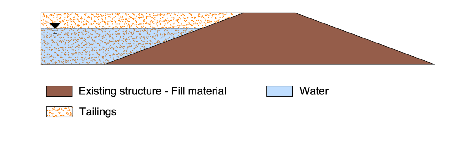
(a)

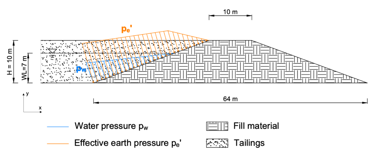
(b)

Figure 2: Initial conditions. (a) Conceptual sketch (b) Loads due to water and tailings as modeled

Loads $\rm{p_{w}}$ and $\rm{p_{e}}$ occur due to water and tailings deposit respectively. They are evaluated as,

$$\rm{p_{w}=\gamma_{w}\times(\rm{WL}-y)}$$ (48)

$$\rm{p_{ex}}=\left\{\begin{array}[]{ll}\rm{K_{a}\big{[}\gamma_{t}(H-WL)+(\gamma_{t}-\gamma_{w})(WL-y)\big{]}}&\rm{\mbox{if }y\leq WL}\\ \rm{K_{a}\gamma_{t}(H-y)}&\rm{\mbox{if }WL<y<H}\end{array}\right.$$ (51)

$$\rm{p_{ey}}=\left\{\begin{array}[]{ll}\rm{\big{[}\gamma_{t}(H-WL)+(\gamma_{t}-\gamma_{w})(WL-y)\big{]}}&\rm{\mbox{if }y\leq WL}\\ \rm{\gamma_{t}(H-y)}&\rm{\mbox{if }WL<y<H}\end{array}\right.$$ (54)

$$\rm{p_{e}}=\sqrt{\rm{p_{ex}}^{2}+\rm{p_{ey}}^{2}}$$ (55)

where $\rm{WL=7m}$ is the water level upstream of the dam and $\rm{H=10m}$ the dam’s height. Specific weights $\rm{\gamma_{w},\gamma_{t}}$ correspond to water and tailings material respectively, $\rm{K_{a}=\frac{1-sin(\phi)}{1+sin(\phi)}}$, is the active earth pressure coefficient, $\phi$ being the tailings’ angle of friction, and $\rm{x,y}$ denote the horizontal and vertical directions.

Following, a load that corresponds to a level raise by $\rm{1m}$ is gradually applied to the top of the structure. The load increases over a duration of 10 days and is then kept constant for the rest of the simulation. This setup is meant to simulate realistic conditions, that is, a small raise, no more than a meter per year, that is preceded and followed by a period of approximately equal time, during which no tailings are deposited, and the fill material is given some time to consolidate. The water table upstream, remains stable throughout the simulation. The final conditions are displayed in Figure 3.

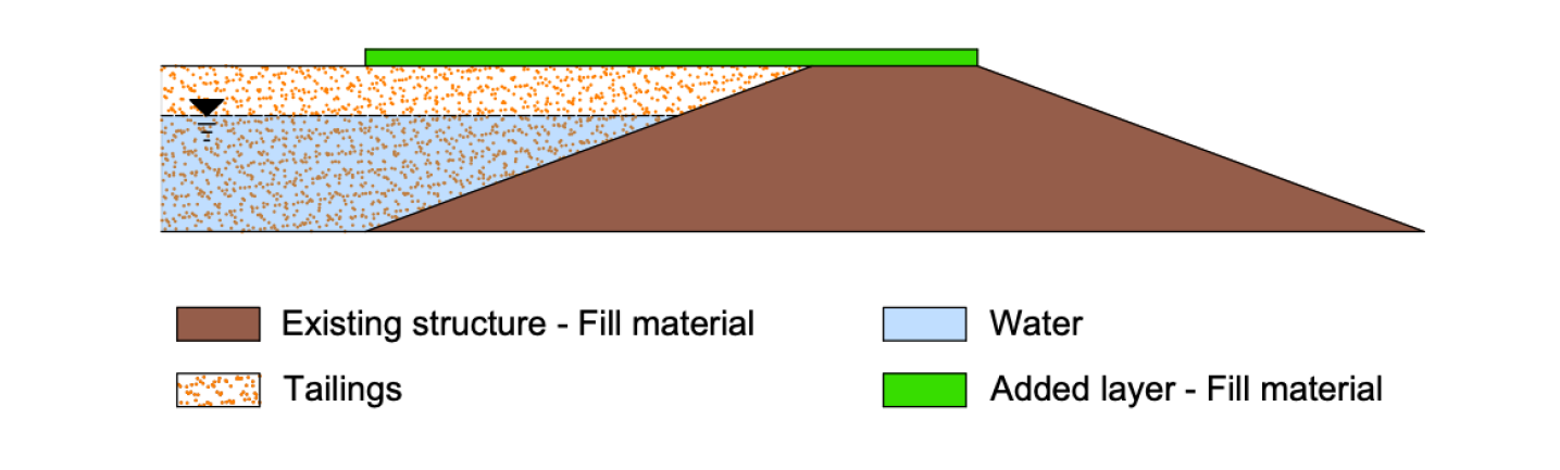
(a)

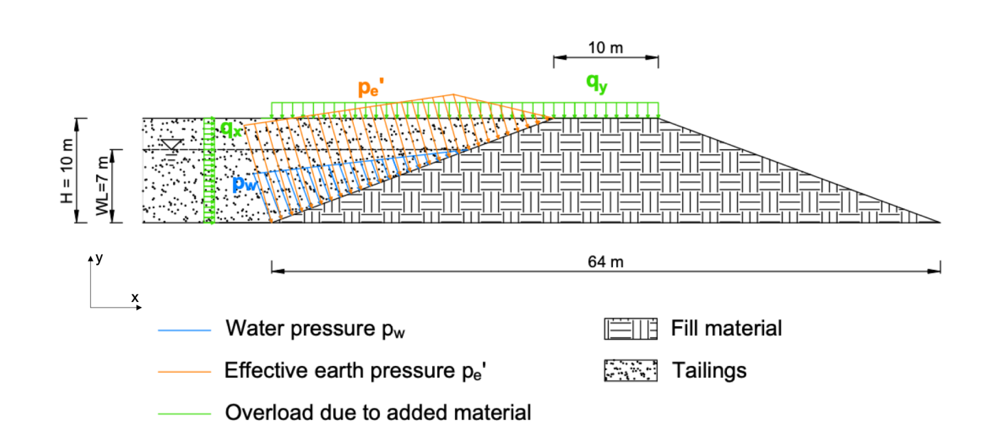
(b)

Figure 3: Final conditions. (a) Conceptual sketch (b) Loads due to water and tailings as modeled

The loads attributed to the 1 meter thick layer of added material are estimated as,

$$\rm{q_{x}=K_{a}\times q_{y}}$$ (56)

$$\rm{q_{y}=\gamma_{f}\times 1m}$$ (57)

where $\rm{\gamma_{f}}$ is the added fill material specific weight.

Therefore the conditions that bound the problem are of type Dirichlet, Newman and Robin. In Figure 4, 5 boundary parts are defined as $\rm{\Gamma_{UD},\Gamma_{UW},\Gamma_{B},\Gamma_{D},\Gamma_{T}}$ that denote Upstream Dry (above water table), Upstream Wet, Bottom, Downstream and Top boundary parts respectively.

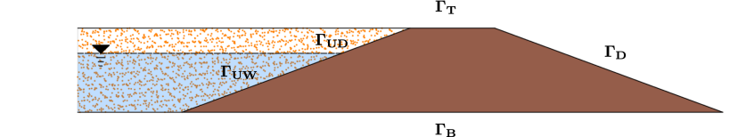
Figure 4: Boundary parts: Upstream Dry, Upstream Wet, Bottom, Downstream, Top

The boundary conditions introduced to the Finite Element model are written as

$$\rm{\mathbf{u}_{x}}=\rm{\mathbf{u}_{y}=0}\quad \text{on}\ \mathbf{\Gamma_{B}}$$ (58)

$$\rm{\boldsymbol{\sigma}\cdot\mathbf{n}}=\rm{\begin{bmatrix}\rm{q_{x}+p_{ex}}&\rm{q_{y}+p_{ey}}\end{bmatrix}^{\intercal}}\quad \text{on}\ \mathbf{\Gamma_{UD}}$$ (59)

$$\rm{\boldsymbol{\sigma}\cdot\mathbf{n}}=\rm{\begin{bmatrix}\rm{q_{x}+p_{wx}+p_{ex}}&\rm{q_{y}+p_{wy}+p_{ey}}\end{bmatrix}^{\intercal}}\quad \text{on}\ \mathbf{\Gamma_{UW}}$$ (60)

$$\rm{\boldsymbol{\sigma}\cdot\mathbf{n}}=\rm{\begin{bmatrix}\rm{0}&\rm{q_{y}}\end{bmatrix}^{\intercal}}\quad \text{on}\ \mathbf{\Gamma_{T}}$$ (61)

$$\rm{p=\gamma_{w}\times(WL-y)}\quad \text{on}\ \mathbf{\Gamma_{UW}}$$ (62)

$$\rm{\mathbf{q}\cdot\mathbf{n}}=\rm{0}\quad \text{on}\ \mathbf{\Gamma_{UD}}\cup\mathbf{\Gamma_{B}}\cup\mathbf{\Gamma_{T}}$$ (63)

$$\rm{\mathbf{q}\cdot\mathbf{n}}=\rm{\langle\beta p\rangle}\quad \text{on}\ \mathbf{\Gamma_{D}}.$$ (64)

The relations among the boundary parts definitions given here, to the ones given in equations (9) - (10) and (13) - (15) may be written $\rm{\Gamma_{D}^{u}}=\mathbf{\Gamma_{B}}$, $\rm{\Gamma_{N}^{u}}=\mathbf{\Gamma_{UD}}\cup\mathbf{\Gamma_{UW}}\cup\mathbf{\Gamma_{T}}$, $\rm{\Gamma_{D}^{p}}=\mathbf{\Gamma_{UW}}$, $\rm{\Gamma_{N}^{p}}=\mathbf{\Gamma_{UD}}\cup\mathbf{\Gamma_{B}}\cup\mathbf{\Gamma_{T}}$, $\rm{\Gamma_{R}^{p}}=\mathbf{\Gamma_{D}}$.

5.2 Implementation: Full and reduced order solvers

A FEM code for the problem stated above was developed in the FEniCS open-source platform. Following, the Reduced Basis method was used to create a low-order solver for the parametrized problem.

The values of the parameters used in the model are given in Tables 1 and 2. The values were chosen such that they fall into ranges that are usually observed in tailings dams (Bhanbhro, 2014) (Qiu and Sego, 2001).

Parameter	Symbol	Units	Value
Gravitational acceleration	$\rm{g}$	$\rm{m/s}$	10
Water bulk modulus	$\rm{K_{w}}$	MPa	$2.2\times 10^{3}$
Specific weight of water	$\rm{\gamma_{w}}$	$\rm{kN/m^{3}}$	$10$
Embankment fill soil material
Particle density	$\rm{\rho_{s}}$	$\rm{kg/m^{3}}$	$2.7\times 10^{3}$
Young’s Modulus	$\rm{E}$	MPa	40
Poisson’s ratio	$\nu$	-	$0.3$
Porosity	$\eta$	-	0.38
Tailings and added fill material
Added fill material specific weight	$\rm{\gamma_{f}}$	$\rm{kN/m^{3}}$	$21$
Tailings specific weight	$\rm{\gamma_{t}}$	$\rm{kN/m^{3}}$	$21$
Tailings friction angle	$\rm{\phi}$	∘	$35$
Van Genuchten Model (van Genuchten, 1980)
Saturated VWC	$\rm{\theta_{s}}$	-	0.38
Residual VWC	$\rm{\theta_{r}}$	-	0.038
Parameter ($\approx$ inverse of air entry suction head)	$\alpha$	$\rm{m^{-1}}$	0.1
Fitting Parameter	$\rm{m}$	-	0.184
Saturated hydraulic conductivity	$\rm{k_{s}}$	$\rm{m/s}$	$\rm{[10^{-9},...10^{-7}]}$

Table 1: Values of physical parameters used in the model

Discretization
Mesh	1382 elements, 774 nodes, unstructured
FE Displacement	P2
FE Pressure	P1
Time integration: $\theta$-scheme
$\theta$	0.75
Time step $\rm{dt}$	0.1 days

Table 2: Numerical parameters used in the model in the 2D scheme

The parameter chosen to be examined is the material saturated hydraulic conductivity $\rm{k_{s}}$. As it has been mentioned above, hydraulic properties of the materials that exist in tailings dams feature high uncertainty and may vary in time. The parametric domain is taken such that the extreme values are realistic in the framework of tailings dams. The saturated hydraulic conductivity of the fill material takes values in $\rm{[10^{-9},...10^{-7}](m/s)}$.

Solving the loading problem with FE

In Figures 5(a)-5(c) the pore water pressure fields acquired by the FE model, solving for $\rm{k_{s}=10^{-9}m/s}$, for 3 different time instances are shown. Figure 5(a) corresponds to the initial state before the loading is applied. Figure 5(b) represents the pore pressure state after 10 days of loading. During the loading time, changes in the displacement field reflect settlement in the dam due to overload. The hydro-mechanical coupling induces an increase of pore pressure, as the material is compressed, and the pore space reduced. Overpressure has been built due to the weight of the added layer of material and the water table has risen. After this point the load ceases to increase and the domain undergoes consolidation as the water table falls. The simulation stops when a steady state is reached. The pressure field is considered to be in steady conditions when the $L_{2}$ norm of the difference between the fields corresponding to two subsequent time steps, is smaller than $\rm{10^{-2}}$. For $\rm{k_{s}=10^{-9}m/s}$ this occurs at $\rm{t=60,6}$ days and the final solution field can be visualized in Figure 5(c).

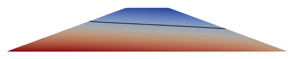
(a)

(b)

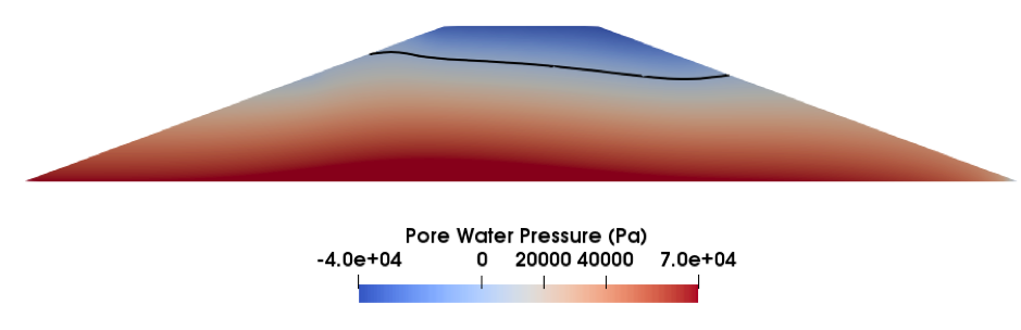
(c)

Figure 5: (a) Initial conditions. Steady state with fixed upstream water table at 7 m (b) At $\rm{t=10}$ days, after 10 days of loading. The maximal overpressure is reached. At this point, the loading stops and pressure starts dissipating. (c) At $\rm{t=60,6}$ days, end of the simulation. The black line indicates the position of the phreatic line.

Setting up the ROM: Offline stage

As explained in section 3, the Reduced Basis is constructed by means of sampling the high-fidelity solution manifold, that is, in this case, the set of solutions obtained by the full-order Finite Element solver.

Specifically, the full order problem was solved for $\rm{k_{s}=[1,3,5,7,10,30,50,70,100]\times 10^{-9}}$, and the solutions were stored in two separate snapshot matrices as in equations (46) and (47). Each of the snapshots have a duration of 10 days, during which the load is applied, plus the time that is needed for steady state conditions to be reached. The time required for steady state conditions to be reached after loading depends on the hydraulic conductivity of the material. The built-up pressure requires longer time to dissipate in a less permeable material. Thus the snapshots have different durations.

Singular value decomposition was applied to the two matrices resulting to the left singular matrix, that was truncated to yield the Reduced Basis. The truncation criterion is based on the singular values. In Figure 6 the singular values that correspond to each of the vectors of the left singular matrix for the two fields are plotted. The y-axis is in logarithmic scale and it is normalized with respect to the first -and largest- singular value. The values drop rapidly in both cases. The first vectors contribute significantly to the description of the solution set, and must, therefore, be included to the Reduced Basis, while as the singular value decreases, the corresponding vectors convey less information about the data, that is, the snapshot matrix

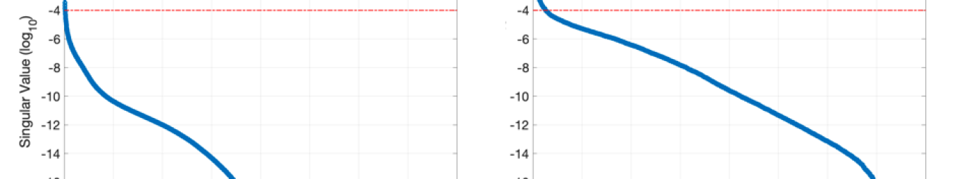
Figure 6: Left singular matrix truncation. Left: Displacement. Right: Pressure

The red dashed line denotes the truncation threshold. In this case, vectors that correspond to singular values that are smaller than the first one by 4 orders of magnitude or more, are discarded. Obtaining a ROM with an accuracy higher than that, would be beyond the scope of the ROM, since the accuracy in the problem is limited by that of the sensor measurements.

This truncation threshold yields a basis that is comprised of just 9 vectors for displacement and 25 for pressure, thus 34 is the size of the reduced system of equations. To put this number of reduced unknowns in perspective, the high-fidelity problem dimension, related to mesh resolution and polynomial degree is 6632 degrees of freedom.

Online stage: Results and comparison

Having populated the transformation matrices $\mathbf{B_{u}}$ and $\mathbf{B_{p}}$, the problem may now be solved, for any parameter within the examined range, by assembling the system of equations and projecting it to the reduced space in which the approximation will be sought, as shown in equation (43). In Figure 7 the relative error of the low order approximation with respect to the high-fidelity solution, is plotted over time. The error is estimated as $\rm{e=\mathinner{\!\left\lvert\frac{X_{RB}-X_{FEM}}{X_{FEM}}\right\rvert}}$, where $\rm{X_{RB}}$ and $\rm{X_{FEM}}$ represent the approximation and the high-fidelity solution respectively.

Of the three values examined in Figure 7, one is a snapshot value, namely $\rm{k_{s}=10^{-8}}\ m/s$, and the other two are values that were not sampled.

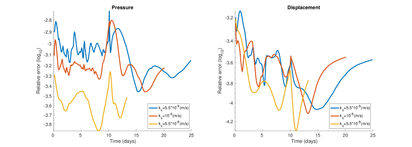
Figure 7: Relative error of low-order approximation of the pressure field with respect to full order solution over time, estimated over the entire domain, for 3 different parametric values. Left: Pressure field. Right: Displacement field.

The errors for both fields and for all parametric values remain quite low, despite the small number of base vectors used. In fact, the error is much lower than the typical accuracy of measurement of the instrumentation that corresponds to the quantities evaluated. Note that the error doesn’t seem to be significantly smaller for the case of the snapshot value $\rm{k_{s}=10^{-8}}\ m/s$. This indicates that the Reduced Basis sufficiently describes the solution states that correspond to the entire spectrum of parametric values. Moreover, it is worth mentioning that the reduced order model yields a small error even for the parametric value that corresponds to a snapshot, which is an expected behavior, considering that the snapshot matrix was truncated after the singular value decomposition.

The ROM runs 3 times faster, by average, than the full-order model. That is a significant boost of computational efficiency, especially considering the relatively low mesh resolution.

To test the effect of mesh resolution to the computational time reduction, another scheme was run, for the same problem, using a denser mesh. In this scheme the high-fidelity system of equations has 2975 degrees of freedom for pressure and 23164 for displacement. The same number of snapshots were taken and corresponded to the same parametric values. The reduced bases that yield the same level of accuracy as the first scheme have 23 base vectors for the pressure field and 9 for the displacement field. The number of vectors needed is very close to the previous scheme, despite the large difference in the size of the high-fidelity problem. In other words, the size of the reduced scheme is decoupled from the size of the high-fidelity scheme (Hesthaven et al., 2016). This is an essential advantage of the Reduced Basis method. It is worth noting that in the case of non-linear problems, like the present, the reduced scheme cannot be fully decoupled from the FEM scheme. Due to the state-dependence of the FEM operators in the linearized system, they have to be reassembled in every iteration of the linearization scheme. The full order system has to be assembled and then transformed into the reduced order one. The assembly of these operators is related to the high-fidelity dimension. Therefore the efficiency gains are bounded. This issue is often addressed by the empirical interpolation methods (Hesthaven et al., 2016)(Quarteroni et al., 2016), the implementation of which, was considered outside the scope of this paper.

5.3 Extension to 3D problems

Literature suggests that 2 dimensional models cannot reflect the complex and variating seepage field (Lyu et al., 2019). Thus, 3 dimensional models have been proposed for the stability study of tailings dams (Lu and Cui, 2006), (Zhang et al., 2020). In this section, a seepage problem, similar to the 2 dimensional one above, will be solved in a 3D setting and a ROM will be developed and evaluated with respect to its accuracy and computational efficiency against the high-fidelity model.

The new geometry approximates an embankment constructed in a narrow, steep sided valley. This is a generic, invented geometry, meant to simulate common conditions in the construction of embankment dams.

In Figure 8 the Y axis indicates the third dimension, while axes X and Z correspond to the dimensions that were considered in the plane strain approximation of the previously solved problem. The domain has a variating cross-section along the Y axis. The two-dimensional domain of the previous setting corresponds to the middle section of the dam, ie the part that has its foundation on the valley (Figure 8(d) Bottom). The parts that are founded on the lateral slopes, have smaller cross sections (Figure 8(d) Top). The side slopes have been assumed excavated in two levels, creating two 5 m-high slopes of inclination 1,5:1. The domain is a 50 m-long prism, has 2 axes of symmetry, and an identical cross-section as the 2D domain shown in Figure 2.

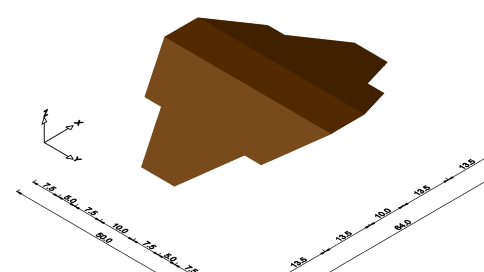
(a) 3D Isometric view

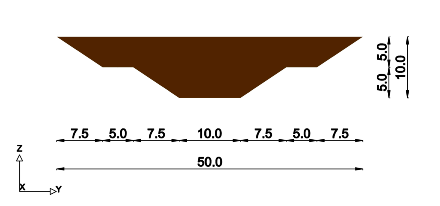
(b) Front view

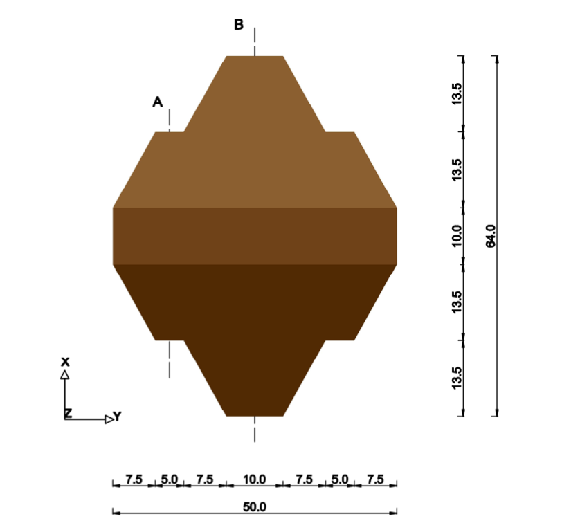
(c) Top view

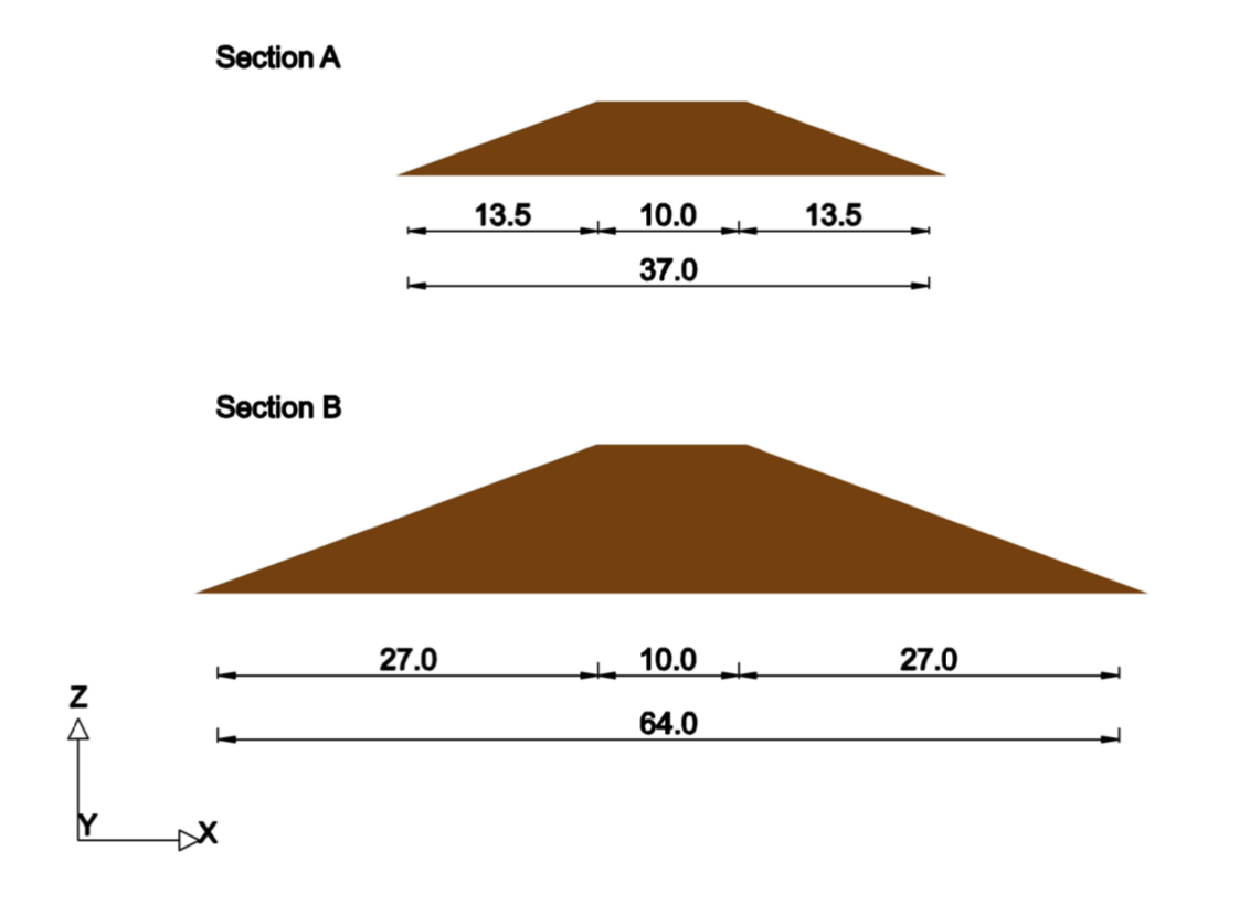
(d) Cross sections Top: Section plane A Bottom: Section plane B

Figure 8: Views and cross sections of the 3 dimensional domain. The geometry assumes an embankment that has been constructed in a narrow valley, and has its foundations on two side slopes at the two extremes in the direction of Y axis. The side slopes are not displayed.

The 3D tetrahedral mesh was created in Gmsh open-source mesh generating software (Geuzaine and Remacle, 2009). The mesh is made out of 41477 tetrahedral and triangular cells and 9896 nodes. Using the Taylor-Hood (P2-P1) element for the description of the displacement and pressure fields as before, the resulting system is comprised of 202179 and 9896 degrees of freedom for the two fields respectively.

As for the problem setup, it remains similar to the 2D case with some alterations. The initial condition is evaluated by solving the steady state problem for an upstream water level at 7 m. The added material is now placed in two layers of 50 cm each. The first layer is deposited in the first 5 days, gradually, across the Y axis. Then the second 50 cm layer is added on top, during days 5-10, again, gradually across the Y axis. After the period of 10 days, the full load that represents the 1m-thick layer remains constant. The bottom boundary is mechanically constrained. The parameters used have the values listed in Table 1. During the level raise phase in a tailings dam’s life, thin layers of fill material are deposited along the length of the structure. The load increases gradually along the 3rd axis of the dam, i.e. the dimension that is not considered in a 2D plane strain approximation. The problem simulates conditions that may occur in the context of an actual tailings dam and cannot be sufficiently approximated in a 2D plane strain setup.

In Figures 9(a) and 9(b) the loading is illustrated for clarity. Two layers of soil are placed on top of the dam, in order to raise the level of the dam by 1 meter in the upstream manner, as shown in Figure 1.

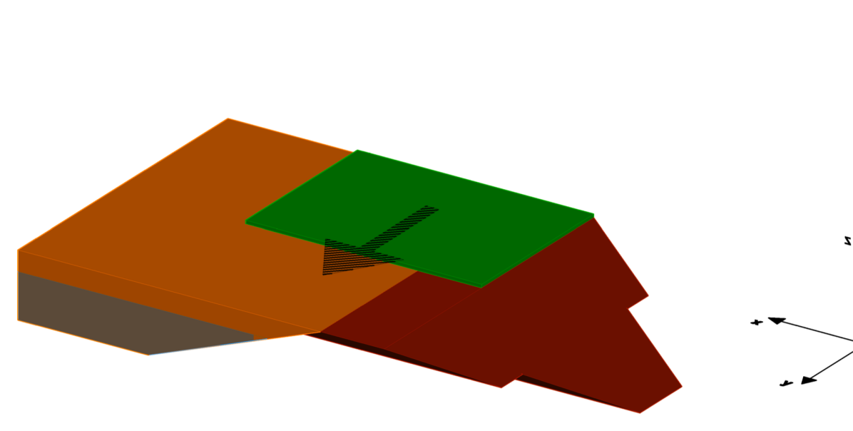
(a) After 2,5 days.

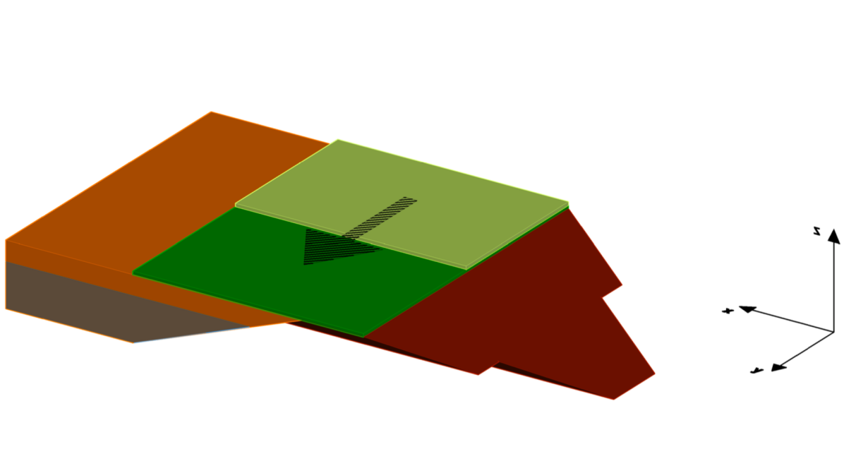
(b) After 7,5 days

Figure 9: Deposition of the two 50 cm - thick layers of fill material on the top and upstream side of the structure. The first layer is shown in dark green color and the second in light green color. After 2,5 days of loading half of the first layer has been deposited. After 7,5 days the first layer and half of the second layer have been deposited. Upstream is in the direction of the x axis. Unsaturated tailings are depicted in orange, saturated tailings in gray. The lateral foundation slopes are not depicted.

In Figure 10, the effect that the gradual load application has on the pore pressure field is illustrated. As the load is applied from one extreme to the other in the y direction, the water table in the area rises to be then lowered after pressure is dissipated through consolidation. By the time the loading procedure is finished after 10 days, in some parts of the dam the water table has almost reached its final position after consolidation.

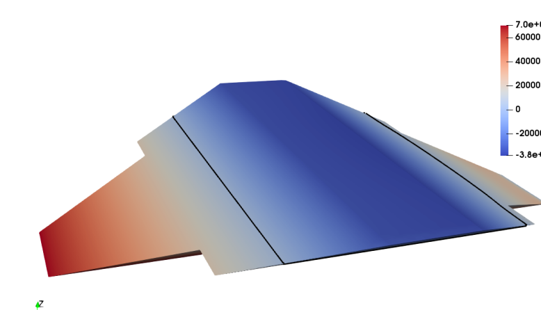
(a) t=0

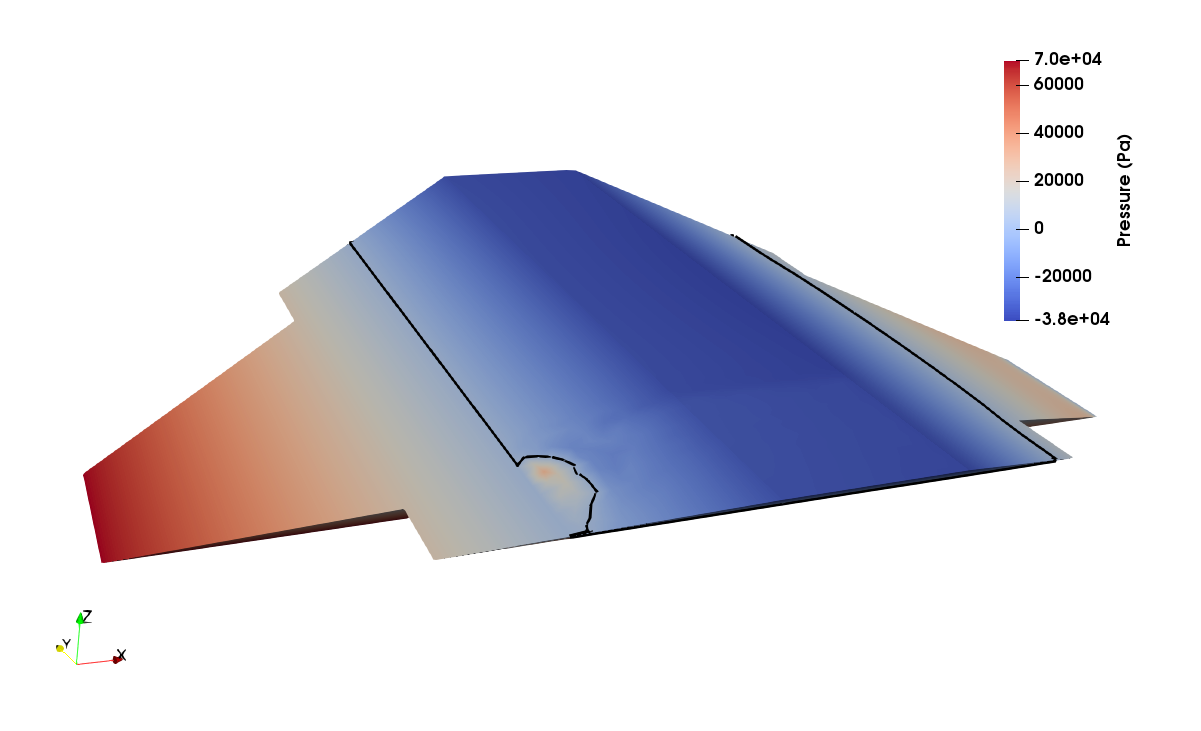
(b) t = 1 day

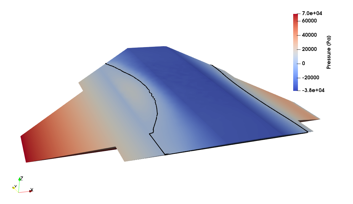
(c) t = 10 days

Figure 10: Pore water pressure distribution on different time instances (a) Initial conditions. Steady state condition with an upstream level at 7m. (b) After 1 day of loading. In some part of the domain overpressure has built up. (c) After 10 days of loading the top of the dam and impoundment. The reservoir is considered to be located on the left side of the figures, i.e. upstream is opposite to the x axis direction.

The Reduced order scheme was created following the same steps as in the 2D case. Snapshots of the high-fidelity solution manifold were taken for parametric values $\rm{k_{s}=[1,3,5,7,10,30,50,70,100]\times 10^{-9}}$. As above, each snapshot has a duration of 10 days of loading, plus the amount of time needed for steady state to be reached in each case. The two solution fields - displacement and pressure- were stored in snapshot matrices $\mathbf{M_{u}}$ and $\mathbf{M}_{\rm{p}}$, arranged as before, i.e. snapshots comprised of all time steps stored in a serial manner in the columns of the matrices. Singular value decomposition was applied to each matrix separately.

Much like in the 2D case, the left singular matrix was truncated with a criterion related to the singular values, admitting only vectors that correspond to singular values up to 4 orders of magnitude smaller than the largest one. The truncation yielded reduced bases comprised of 80 base vectors for displacement and 174 for pressure. Therefore the system of equations to be solved now is of dimensionality 214, instead of the full order problem with 212075 degrees of freedom.

The same parametric values as before were examined in order to estimate the accuracy and computational efficiency gain of the RB approximation. In Figure 11 the $L_{2}$ norms of the relative error -estimated as the difference between full order and reduced order solutions- have been plotted for the two fields.

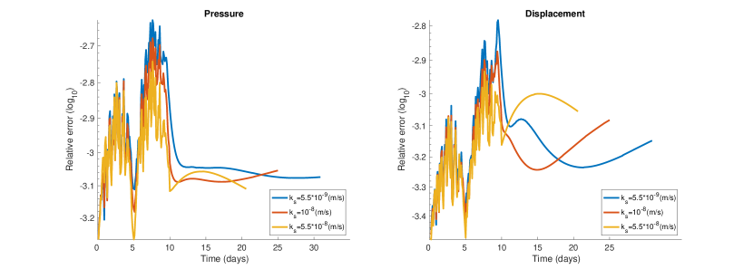
Figure 11: Relative error of low-order approximation of the pressure field with respect to full order solution over time, estimated over the entire 3D domain, for 3 different parametric values. Left: Pressure field. Right: Displacement field.

In comparison to the 2D scheme, it seems that the ROM yields slightly lower accuracy, which remains however in the same order of magnitude. The accuracy can easily be improved by choosing a smaller truncation tolerance for the reduced basis. For various parametric values that were tested, the ROM was found to run 8 - 15 times faster than the full-order model. This is a significant increase of gain in computational efficiency compared to the 2D case, which indicates that the time gain scales along with the size of the problem at hand.

6 Conclusions and future work

In this work a low order model for the hydro-mechanically coupled problem has been developed, using the Reduced Basis technique. The POD-based method has been successfully applied. A first attempt to treat the parametrized system of PDEs and confirming a high level of accuracy has been demonstrated. The computational time needed is reduced in this simplified problem, while the accuracy of the solution is not compromised, in comparison to the full-order Finite Element solution. The method is promising, considering that the time reduction increases with increasing problem size.

It is worth noting that in the framework of tailings dams the usual practice is to model the retaining structure as well as the stored material, due to the fact that failure may originate in the impoundment. Sufficiently describing the pressure and displacement field -or other fields of interest- in such a large inhomogeneous domain can result in large systems, in which case the advantages of a reduced order model would be most prominent.

As it has been pointed out in this paper, computational efficiency is key for solving inverse problems, such as parameter identification in real-time, or near real-time. Enabling fast many-query solutions may contribute heavily to predictive monitoring applications in earthfil dams. On that note, the continuation of this work is likely to involve data assimilation applications and inverse problem solving for tailings dams.

The most straightforward step for the future of this work is the implementation of hyper-reduction techniques in order to treat the non-linear matrix and vector terms of the system, thus achieving higher computational efficiency. One quite promising method is the Discrete Empirical Interpolation (DEIM) proposed in (Chaturantabut and Sorensen, 2010) and extended for treatment of matrix non-linear operators in (Negri et al., 2015). The method aims at identifying reduced approximations of nonlinear functions in a POD manner and has been successfully applied to coupled problems treated with FEM (Santo and Manzoni, 2019).

Another issue to be explored is high-dimensionality in the parametric domain. In tailings dams, parameters related to both the mechanical and hydraulic problems may feature high uncertainty and may fluctuate significantly as the structure evolves. Therefore, updating the model for multiple parameters as their values change is a relevant problem, and one that accentuates the need for order reduction in an inverse problem context.

7 Acknowledgements

This work has received funding from the European Union’s Horizon 2020 research and innovation programme under the Marie Sklodowska-Curie grant agreement No 764636, for the research project ProTechTion.

We thank Professor Sebatian Olivella (Escola de Camins, Universitat Politècnica de Catalunya) for his much appreciated assistance.

Pedro Díez and Sergio Zlotink are grateful for the financial support provided by the Spanish Ministry of Economy and Competitiveness (Grant agreement No. DPI2017-85139-C2-2-R), by the Generalitat de Catalunya (Grant agreement No. 2017-SGR-1278), and by project H2020-RISE MATH-ROCKS GA no 777778.

References

References

-
Alnaes et al. (2015)
Alnaes, M. S., B. Kehlet, A. Logg, C. Richardson, J. Ring, E. Rognes, and G. N.
Wells
2015. The FEniCS Project Version 1.5. P. 15. -
Alonso et al. (2005)
Alonso, E. E., S. Olivella, and N. M. Pinyol
2005. A review of Beliche Dam. Géotechnique, 55(4):267–285. -
Badia et al. (2009)
Badia, S., A. Quaini, and A. Quarteroni
2009. Coupling Biot and Navier–Stokes equations for modelling fluid–poroelastic media interaction. Journal of Computational Physics, P. 29. -
Bao et al. (2019)
Bao, A., E. Gildin, A. Narasingam, and J. S.
Kwon
2019. Data-Driven Model Reduction for Coupled Flow and Geomechanics Based on DMD Methods. Fluids, 4(3):138. -
Bhanbhro (2014)
Bhanbhro, R.
2014. Mechanical Properties of Tailings: Basic Description of a Tailings Material from Sweden. Publisher: Unpublished. -
Chaturantabut and
Sorensen (2010)
Chaturantabut, S. and D. C. Sorensen
2010. Nonlinear Model Reduction via Discrete Empirical Interpolation. SIAM Journal on Scientific Computing, 32(5):2737–2764. -
Clarkson et al. (2020)
Clarkson, L., D. Williams, and J. Seppälä
2020. Real-time monitoring of tailings dams. Georisk: Assessment and Management of Risk for Engineered Systems and Geohazards, Pp. 1–15. -
Davies and Martin (2002)
Davies, M. and T. Martin
2002. Static liquefaction of tailings–fundamentals and case histories. In Proceedings of Tailings Dams ASDSO/USCOLD, Pp. 233–255, Las Vegas 2002. -
Esmaeili et al. (2020)
Esmaeili, M., M. Ahmadi, and A. Kazemi
2020. A generalized DEIM technique for model order reduction of porous media simulations in reservoir optimizations. Journal of Computational Physics, 422:109769. -
Florentin and
Díez (2012)
Florentin, E. and P. Díez
2012. Adaptive reduced basis strategy based on goal oriented error assessment for stochastic problems. Comput. Methods Appl. Mech. Engrg., P. 12. -
Gerard et al. (2009)
Gerard, P., A. Leonard, J.-P. Masekanya, R. Charlier, and
F. Collin
2009. Study of the soil-atmosphere moisture exchanges through convective drying tests in non-isothermal conditions. P. 24. -
Geuzaine and Remacle (2009)
Geuzaine, C. and J.-F. Remacle
2009. Gmsh: A 3-D finite element mesh generator with built-in pre- and post-processing facilities: THE GMSH PAPER. International Journal for Numerical Methods in Engineering, 79(11):1309–1331. -
Ghommem et al. (2016)
Ghommem, M., E. Gildin, and M. Ghasemi
2016. Complexity Reduction of Multiphase Flows in Heterogeneous Porous Media. SPE Journal, 21(01):144–151. -
Gildin et al. (2013)
Gildin, E., M. Ghasemi, A. Romanovskay, and
Y. Efendiev
2013. Nonlinear Complexity Reduction for Fast Simulation of Flow in Heterogeneous Porous Media. In All Days, Pp. SPE–163618–MS, The Woodlands, Texas, USA. SPE. -
Hamade (2013)
Hamade, T.
2013. Geotechnical Design of Tailings Dams - A Stochastic Analysis Approach. PhD thesis, McGill University. -
Heshmati R.
et al. (2020)
Heshmati R., A. A., H. Salehzadeh, and
M. Shahidi
2020. Prediction of the Void Ratio Parameter in Mineral Tailings Using Gene Expression Programming. Advances in Civil Engineering, 2020:1–12. -
Hesthaven et al. (2016)
Hesthaven, J. S., G. Rozza, and B. Stamm
2016. Certified Reduced Basis Methods for Parametrized Partial Differential Equations, SpringerBriefs in Mathematics. Cham: Springer International Publishing. -
Hoang et al. (2018)
Hoang, K. C., T.-Y. Kim, and J.-H. Song
2018. Fast and accurate two-field reduced basis approximation for parametrized thermoelasticity problems. Finite Elements in Analysis and Design, 141:96–118. -
Hui et al. (2018)
Hui, S. R., L. Charlebois, and C. Sun
2018. Real-time monitoring for structural health, public safety, and risk management of mine tailings dams. Canadian Journal of Earth Sciences, 55(3):221–229. -
Knutsson et al. (2016)
Knutsson, R., A. Bjelkevik, and S. Knutsson
2016. Slope stability in landform design. In Proceedings of the 11th International Conference on Mine Closure, A. Fourie and M. Tibbett, eds., Pp. 89–98. Australian Centre for Geomechanics. event-place: Perth. -
Kossoff et al. (2014)
Kossoff, D., W. Dubbin, M. Alfredsson, S. Edwards, M. Macklin, and
K. Hudson-Edwards
2014. Mine tailings dams: Characteristics, failure, environmental impacts, and remediation. Applied Geochemistry, 51:229–245. -
Larion et al. (2020)
Larion, Y., S. Zlotnik, T. Massart, and P. Díez
2020. Building a certified reduced basis for coupled thermo-hydro-mechanical systems with goal-oriented error estimation. Computational Mechanics, 66. -
Lu and Cui (2006)
Lu, M.-l. and L. Cui
2006. Three-dimensional seepage analysis for complex topographical tailings dam. Yantu Lixue(Rock and Soil Mechanics), 27(7):1176–1180. -
Lyu et al. (2019)
Lyu, Z., J. Chai, Z. Xu, Y. Qin, and J. Cao
2019. A Comprehensive Review on Reasons for Tailings Dam Failures Based on Case History. Advances in Civil Engineering, 2019:1–18. -
Maday and Ronquist (2004)
Maday, Y. and E. M. Ronquist
2004. The Reduced Basis Element Method: Application to a Thermal Fin Problem. SIAM Journal on Scientific Computing, 26(1):240–258. -
Maday and
Rønquist (2002)
Maday, Y. and E. M. Rønquist
2002. A reduced-basis element method. Comptes Rendus Mathematique, 335(2):195–200. -
Martin and
McRoberts (1999)
Martin, T. E. and E. C. McRoberts
1999. Some considerations in the stability analysis of upstream tailings dams. P. 18. -
Morton (2021)
Morton, K. L.
2021. The Use of Accurate Pore Pressure Monitoring for Risk Reduction in Tailings Dams. Mine Water and the Environment, 40(1):42–49. -
Negri et al. (2015)
Negri, F., A. Manzoni, and D. Amsallem
2015. Efficient model reduction of parametrized systems by matrix discrete empirical interpolation. Journal of Computational Physics, 303:431–454. -
Nuth and Laloui (2008)
Nuth, M. and L. Laloui
2008. Effective stress concept in unsaturated soils: Clarification and validation of a unified framework. International Journal for Numerical and Analytical Methods in Geomechanics, 32(7):771–801. -
Ortega‐Gelabert
et al. (2020)
Ortega‐Gelabert, O., S. Zlotnik, J. C. Afonso, and
P. Díez
2020. Fast Stokes Flow Simulations for Geophysical‐Geodynamic Inverse Problems and Sensitivity Analyses Based On Reduced Order Modeling. Journal of Geophysical Research: Solid Earth, 125(3):25. -
Pinyol et al. (2008)
Pinyol, N. M., E. E. Alonso, and S. Olivella
2008. Rapid drawdown in slopes and embankments. Water Resources Research, 44(5). -
Qiu and Sego (2001)
Qiu, Y. J. and D. C. Sego
2001. Laboratory properties of mine tailings. Canadian Geotechnical Journal, 38(1):183–190. -
Quarteroni et al. (2016)
Quarteroni, A., A. Manzoni, and F. Negri
2016. Reduced Basis Methods for Partial Differential Equations, volume 92 of UNITEXT. Cham: Springer International Publishing. -
Quarteroni and
Rozza (2014)
Quarteroni, A. and G. Rozza, eds.
2014. Reduced Order Methods for Modeling and Computational Reduction. Cham: Springer International Publishing. -
Rozza et al. (2007)
Rozza, G., D. B. P. Huynh, and A. T. Patera
2007. Reduced basis approximation and a posteriori error estimation for affinely parametrized elliptic coercive partial differential equations. Archives of Computational Methods in Engineering, 15(3):1–47. -
Saad and Mitri (2011)
Saad, B. and H. Mitri
2011. Hydromechanical Analysis of Upstream Tailings Disposal Facilities. Journal of Geotechnical and Geoenvironmental Engineering, 137(1):27–42. -
Santo and
Manzoni (2019)
Santo, N. D. and A. Manzoni
2019. Hyper-reduced order models for parametrized unsteady Navier-Stokes equations on domains with variable shape. Advances in Computational Mathematics, 45(5-6):2463–2501. -
Szostak et al. (2003)
Szostak, A., A. Chrzanowski, and M. Massiéra
2003. Use of geodetic monitoring measurements in solving geomechanical problems in structural and mining engineering. P. 9, Santorini, Greece. -
van Doren
et al. (2006)
van Doren, J. F. M., R. Markovinović, and J.-D.
Jansen
2006. Reduced-order optimal control of water flooding using proper orthogonal decomposition. Computational Geosciences, 10(1):137–158. -
van
Genuchten (1980)
van Genuchten, M. T.
1980. A Closed-form Equation for Predicting the Hydraulic Conductivity of Unsaturated Soils. Soil Science Society of America Journal, 44(5):892–898. -
Vanden Berghe
et al. (2011)
Vanden Berghe, J.-F., J.-C. Ballard, J.-F. Wintgens, and
B. List
2011. Geotechnical Risks Related to Tailings Dam Operations. In Tailings and Mine Waste Conference (2011 : Vancouver, B.C.), P. 11. -
Vermeulen et al. (2004)
Vermeulen, P., A. Heemink, and C. Te Stroet
2004. Reduced models for linear groundwater flow models using empirical orthogonal functions. Advances in Water Resources, 27(1):57–69. -
Villavicencio
et al. (2011)
Villavicencio, A. G., P. Breul, C. Bacconnet, D. Boissier, and A. R.
Espinace
2011. Estimation of the Variability of Tailings Dams Properties in Order to Perform Probabilistic Assessment. Geotechnical and Geological Engineering, 29(6):1073–1084. -
Zhang et al. (2020)
Zhang, C., J. Chai, J. Cao, Z. Xu, Y. Qin, and
Z. Lv
2020. Numerical Simulation of Seepage and Stability of Tailings Dams: A Case Study in Lixi, China. Water, 12(3):742.