Ensemble Markov chain Monte Carlo with teleporting walkers

Abstract

We introduce an ensemble Markov chain Monte Carlo approach to sampling from a probability density with known likelihood. This method upgrades an underlying Markov chain by allowing an ensemble of such chains to interact via a process in which one chain’s state is cloned as another’s is deleted. This effective teleportation of states can overcome issues of metastability in the underlying chain, as the scheme enjoys rapid mixing once the modes of the target density have been populated. We derive a mean-field limit for the evolution of the ensemble. We analyze the global and local convergence of this mean-field limit, showing asymptotic convergence independent of the spectral gap of the underlying Markov chain, and moreover we interpret the limiting evolution as a gradient flow. We explain how interaction can be applied selectively to a subset of state variables in order to maintain advantage on very high-dimensional problems. Finally we present the application of our methodology to Bayesian hyperparameter estimation for Gaussian process regression.

65C05, 62F15, 60J85

1 Introduction

In practice, the efficiency of a Markov chain Monte Carlo (MCMC) algorithm is often limited by metastability, that is, the need to repeatedly transition between high-probability regions separated by regions of low probability. Because an MCMC chain is designed to sample each region according to its probability, it will necessarily visit the low-probability region, and therefore also transition between the high-probability regions, only infrequently. In practice, metastability is difficult to address without detailed insights into its origins in the specific problem of interest (e.g., a description of relatively high-probability pathways connecting high-probability regions). Common approaches to overcoming metastability involve the modification of a general-purpose MCMC algorithm (such as Metropolis–Hastings or Langevin dynamics [22, 17]) by, e.g., rescaling the log target density by a small factor (as in parallel tempering [22, 9]) or stratifying the sampling space (as in umbrella sampling [8, 24] and related schemes [5, 30]).

We propose an alternative strategy in which an interaction is introduced between multiple (otherwise independently evolving) chains, specifying the evolution for an ensemble of ‘walkers.’ At each step of the algorithm, one walker is selected to be duplicated and moved according to some proposal, and another is selected to be removed. If the duplicated and removed walkers are different, we say that a walker has been ‘teleported.’ The scheme involves a Metropolis–Hastings accept-reject step and exactly preserves a specified target density. In the mean-field limit of many walkers, the acceptance probability converges to 1, and our scheme somewhat resembles a resampling strategy [6]. We identify the mean-field evolution and find that its local convergence to the target is rapid even in cases that would lead to metastabilities in standard single-chain MCMC schemes. In particular, we prove an asymptotic convergence rate for the mean-field evolution that is independent of the spectral gap of the Markov chain used to define the parallel walker evolutions. Moreover, we interpret the mean-field density evolution as a gradient flow [1] of the $\chi^{2}$-divergence [21] with respect to a metric that resembles the Hellinger distance [21].

A shortcoming of our scheme is that the advantage from interaction tends to decrease as the dimension of the sample space increases relative to the number of walkers. Fortunately, in this limit our scheme reverts to running independent chains sampling from the target without interaction. Moreover, as we demonstrate, for higher-dimensional sampling problems the interaction we introduce can be restricted to a low-dimensional subspace of state variables.

Ensemble Markov chain Monte Carlo schemes are now implemented in several very popular software packages and have found widespread use on a variety of parameter estimation problems [10, 32]. Most of these schemes use information from the ensemble of chains to address conditioning problems [13, 4, 7, 14, 15, 18], i.e., they increase the size of the updates for each chain in directions in which $\pi$ decays relatively slowly, while several articles have emphasized the use of ensemble schemes to avoid gradient evaluations in traditional optimization and sampling tasks [11, 12, 25, 26]. Recently, studies of the mean-field limit of such schemes have yielded useful new insights [11, 12, 26]. Meanwhile, it seems that comparatively few ensemble schemes have been proposed to address slow MCMC convergence due to metastability. In that our ensemble scheme yields a nonlinear mean-field evolution, it is related to the ‘nonlinear’ MCMC schemes discussed in [3]. It is more closely related to the ensemble Langevin sampler with birth and death introduced in [23], though that scheme involves additional parameter-dependent approximations. Similar birth and death dynamics were introduced in [27] to accelerate training of neural network parameters.

This article is organized as follows. In Section 2, we introduce our ensemble scheme. In Section 3, we formally derive the continuum evolution that emerges in the limit of a large number of walkers, proving global convergence to the target with an asymptotic rate that is independent of the spectral gap of the underlying single-walker Markov chain. We also interpret the evolution as a gradient flow. In Section 4, we explain how our scheme can be adapted to introduce interaction only among a subset of state variables. In Section 5, we conclude with numerical experiments. Specifically, we provide a simple illustration of the continuum evolution, and we demonstrate practical performance of our ensemble scheme on Bayesian hyperparameter estimation problems for Gaussian process regression. Under a non-Gaussian measurement noise model, the resulting sampling problem is very high-dimensional and requires us to introduce walker interaction only among a naturally chosen subset of state variables.

2 Interacting walker proposal

Suppose that we are given (up to a possibly unknown normalization) a probability density $\pi(x)$ on a space $X$ and a Markov chain transition density $q(y\,|\,x)$ that might serve as a good proposal within a Metropolis–Hastings scheme sampling the target $\pi$. We want to lift such an approach to an interacting walker approach on the $N$-fold product space $X^{N}$. Specifically, for a fixed walker number $N$, we want to sample $\mathbf{x}=(x_{1},\ldots,x_{N})\in X^{N}$ from the probability measure $dM(\mathbf{x})\propto\Pi(\mathbf{x})\,d\mathbf{x}$, where

$$\Pi(\mathbf{x})=\prod_{i=1}^{N}\pi(x_{i}).$$

Though the variables $x_{1},\ldots,x_{N}$ are independent with respect to the joint measure $\Pi$, our chain on $X^{N}$ will not decouple into $N$ independent chains on $X$.

Note that to any $\mathbf{x}\in X^{N}$ we can associate the empirical measure $\nu(\mathbf{x})=\frac{1}{N}\sum_{i=1}^{N}\delta_{x_{i}}$. For bounded continuous $\phi:X\rightarrow\mathbb{R}$ and Borel probability measures $\nu$, we define $\left\langle\phi,\nu\right\rangle=\mathbb{E}_{\nu}\left[\phi\right]$. Then we may compute any expectation with respect to the original target measure $\mu$ as

$$\mathbb{E}_{x\sim\mu}\left[\phi(x)\right]=\mathbb{E}_{\mathbf{x}\sim M}\left[\left\langle\phi,\nu(\mathbf{x})\right\rangle\right],$$

provided that we can sample from $M$.

Consider the following proposal for an update $\mathbf{x}\rightarrow\mathbf{x}^{\prime}$. First uniformly select $j\in\{1,\ldots,N\}$. In our proposal, the $j$-th sample will be cloned and then moved according to $q$, and we then sample an index $i$ (possibly equal to $j$) for a sample to delete from our original set of samples. As such, sample $z\sim q(\,\cdot\,|\,x_{j})$. The index $i$ is then sampled according to the importance weights

$$w_{i}(\mathbf{x},z):=\frac{q(x_{i}\,|\,z)+\sum_{k\neq i}^{N}q(x_{i}\,|\,x_{k})}{\pi(x_{i})}\Bigg{/}Z(\mathbf{x},z),$$

where

$$Z(\mathbf{x},z):=\sum_{l=1}^{N}\frac{q(x_{l}\,|\,z)+\sum_{k\neq l}^{N}q(x_{l}\,|\,x_{k})}{\pi(x_{l})}.$$

Notice that if $\mathcal{Q}$ is the transition operator on probability measures induced by $q$, i.e., for a probability measure $\mu$,

$$\mathcal{Q}\mu(dy)=\int q(dy\,|\,x)\,d\mu(x),$$

then the numerator $q(x_{i}\,|\,z)+\sum_{k\neq i}^{N}q(x_{i}\,|\,x_{k})$ appearing in the preceding expressions is the density of the measure $\mathcal{Q}\left[\delta_{z}+\sum_{k\neq i}\delta_{x_{k}}\right]$ evaluated at $x_{i}$. Hence it is improbable to select $i$ for deletion unless $x_{i}$ is ‘close’ to one of the other samples, i.e., to some $y\in\{x_{1},\ldots,x_{N},z\}\backslash\{x_{i}\}$, in the sense that $q(x_{i}\,|\,y)$ is nonnegligible. Then having sampled $i$, the proposal is given by $\mathbf{x}^{\prime}=(x_{k}^{\prime})$, where $x_{k}^{\prime}=x_{k}$ for all $k\neq i$, $x_{i}^{\prime}=z$. In other words, $x_{i}$ is replaced by $z$ in the proposal.

Supposing that we have generated $\mathbf{x^{\prime}}$ via the procedure described above (i.e., so that $i$, $j$, and $z$ are defined as above), the Metropolis-Hastings acceptance probability can be computed as

$$\min\left(1,\frac{Z(\mathbf{x},z)}{Z(\mathbf{x}^{\prime},x_{i})}\right).$$

(See Appendix A for a detailed calculation.) Observe that if none of the walkers are close to one another according to $q$, i.e., if $q(x_{l}|x_{k})\approx 0$ for all $k\neq l$ and moreover $q(x_{l}|z)\approx 0$ for all $l\neq j$, then we select $i=j$ with high probability, and the acceptance probability is approximately

$$\min\left(1,\frac{q(x_{j}\,|\,z)}{\pi(x_{j})}\frac{\pi(z)}{q(z\,|\,x_{j})}\right),$$

so we default to simply performing a Metropolis update according to $q$ for the $j$-th sample.

Meanwhile, as we shall discuss in more detail below, one expects $Z(\mathbf{x},z)\approx Z(\mathbf{x}^{\prime},x_{i})$ when the number of walkers is large. In other words, we expect that the acceptance probability will approach $1$ as the number of samples is increased, holding all else constant.

As $N$ increases, one expects a transition from the small-$N$ regime (in which the walkers are isolated from one another relative to the proposal kernel) to the large-$N$ regime (in which each walker has several neighbors relative to the kernel). A curse of dimensionality enters in that for a fixed proposal kernel that is narrow enough to yield a nonnegligible acceptance probability, one must take $N$ exponentially large in the dimension of $X$ in order for each walker to have several neighbors with respect to this kernel. However, the onset of the curse is delayed as the proposal is improved; indeed, if $q(y\,|\,x)=\pi(y)$, then by inspection one observes that the importance weights $w_{i}$ are uniform, the acceptance probability is $1$, and the sampler reaches equilibrium in one step, just as is the case for ordinary MCMC with a perfect proposal. In practice, we shall observe that the scheme can still succeed on practical problems in dimensions that are much too high to treat simply by quadrature.

3 Large-$N$ limit

In this section we consider the scheme introduced in Section 2 in the limit of large $N$. In this limit we will try to identify the empirical measure $\nu=\nu(\mathbf{x})$ with an absolutely continuous measure $d\nu=\rho\ dx$. In this section we provide a formal derivation of the dynamics that emerge for $\rho$ in this limit. Note that since each update step can only move a single walker, we only make a change of order $1/N$ to $\nu$. Hence we want to think of $\Delta t=1/N$.

Notice that if $d\nu\approx\rho\,dx$, we can approximate

$$\frac{Z(\mathbf{x},z)}{N^{2}}\approx\frac{Z(\mathbf{x}^{\prime},x_{i})}{N^{2}}\approx\mathbb{E}_{x\sim\nu}\left[\frac{1}{\pi(x)}\frac{d(\mathcal{Q}\nu)}{dx}\right]=\int\frac{\mathcal{Q}\rho(x)}{\pi(x)}\rho(x)\,dx,$$

where we abuse notation slightly to view $\mathcal{Q}$ is an operator on probability densities as well as measures, i.e., we define $\mathcal{Q}p(x)=\frac{d(\mathcal{Q}\mu)}{dx}$ where $p$ is the density of $\mu$. Note that in particular we expect the acceptance probability converges to $1$ as $N\rightarrow\infty$.

Consider $\phi:X\rightarrow\mathbb{R}$. Then for $\mathbf{x}$ fixed and $\mathbf{x}^{\prime}$ (random) obtained by applying one step of our chain to $\mathbf{x}$, we have

$$\mathbb{E}\left(\left\langle\phi,\nu(\mathbf{x}^{\prime})-\nu(\mathbf{x})\right\rangle\right)\approx\frac{1}{N}\mathbb{E}\left\{\phi(z)-\phi(x_{i})\right\}$$

for large $N$, since the acceptance probability is approximately $1$. In the right-hand side, $z$ is sampled by sampling $y\sim\nu(\mathbf{x})$ and then applying one step of $q$ to obtain $z$, i.e., $z$ is sampled from the density $\mathcal{Q}\rho$, and the index $i$ is sampled according to the importance weight

$$w_{i}(\mathbf{x},z):=\frac{q(x_{i}\,|\,z)+\sum_{k\neq i}^{N}q(x_{i}\,|\,x_{k})}{\pi(x_{i})}\Bigg{/}Z(\mathbf{x},z)\approx\frac{\frac{\mathcal{Q}\rho(x_{i})}{\pi(x_{i})}}{\int\frac{\mathcal{Q}\rho(x)}{\pi(x)}\rho(x)\,dx}.$$

Hence we can view $y:=x_{i}$ as being approximately sampled from the importance-weighted density $\frac{1}{Z_{p}}\frac{\mathcal{Q}\rho}{\pi}\rho$, where $Z_{\rho}:=\int\frac{\mathcal{Q}\rho(x)}{\pi(x)}\rho(x)\,dx$, and therefore

$$\frac{\mathbb{E}\left(\left\langle\phi,\nu(\mathbf{x}^{\prime})-\nu(\mathbf{x})\right\rangle\right)}{\Delta t} \approx \int\phi(z)\,\mathcal{Q}\rho(z)\,dz-\frac{1}{Z_{\rho}}\int\phi(y)\frac{\mathcal{Q}\rho(y)}{\pi(y)}\rho(y)\,dy$$

$$= \int\phi(x)\,\left[1-\frac{1}{Z_{\rho}}\frac{\rho(x)}{\pi(x)}\right]\mathcal{Q}\rho(x)\,dy.$$

Now we view $\frac{\mathbb{E}\left(\left\langle\phi,\tilde{\nu}-\nu\right\rangle\right)}{\Delta t}\approx\left\langle\phi,\dot{\rho}\right\rangle_{L^{2}}$, where we view $\rho=\rho_{t}(x)$ now as time-dependent and take $\dot{\rho}_{t}(x)=\frac{\partial}{\partial t}\rho_{t}(x)$, so we infer

$$\dot{\rho}_{t}(x)=\frac{1}{Z_{\rho_{t}}}\left[Z_{\rho_{t}}-\frac{\rho_{t}(x)}{\pi(x)}\right]\mathcal{Q}\rho_{t}(x).$$

For simplicity we shall often write $\rho=\rho_{t}$ and even omit dependence on $x$, as in

(3.1) $$\dot{\rho}=\frac{1}{Z_{\rho}}\left[Z_{\rho}-\frac{\rho}{\pi}\right]\mathcal{Q}\rho.$$

3.1 Global convergence analysis

Our goal in this section is to analyze the convergence of the dynamics (3.1) to the target density $\pi$. We also highlight the constrast with the dynamics that arise from considering $N$ independent Markov chains, each with transition $\tilde{\mathcal{Q}}$ defined to be the Metropolized version of $\mathcal{Q}$, which satisfies $\tilde{\mathcal{Q}}\pi=\pi$. These dynamics are specified by

(3.2) $$\dot{\rho}=-\left(\mathrm{Id}-\tilde{\mathcal{Q}}\right)\rho,$$

as can be verified by an analogous (but simpler) formal calculation. Equivalently, we have $\dot{\eta}=-\left(\mathrm{Id}-\tilde{\mathcal{Q}}\right)\eta,$ where $\eta:=\rho-\pi$. These dynamics for the error conserve the constraint $\int\eta\,dx=0$. On the subspace defined by this constraint, the convergence of the dynamics is linear with rate given by the spectral gap of $\tilde{\mathcal{Q}}$ [20]. Hence the convergence is slow when the gap is small, which is known to be the case [19, 16], e.g., for multimodal $\pi$ with local proposals that cannot cross between modes.

Our ensemble approach cannot ‘discover’ new modes any faster than would an independent-chain approach. This is intuitive from the construction, as well as the perspective of Section 3.3 below, which can be viewed in part as quantifying the difficulty of expanding the support of $\rho$. However, once the modes are discovered, the convergence is potentially much faster, as our local convergence analysis of the continuum limit shall indicate. By contrast, note that for independent walkers, even if all modes are populated by the ensemble, fluctuations in the populations of each mode will dissipate very slowly, leading to very slow convergence.

We approach questions of convergence first by identifying a convenient monotone quantity, defined as a Pearson $\chi^{2}$-divergence. Recall that this divergence is defined by the formula [21]

$$\chi^{2}(\rho_{1}\,\|\,\rho_{2}):=\int\left(1-\frac{\rho_{1}(x)}{\rho_{2}(x)}\right)^{2}\rho_{2}(x)\,dx=\int\frac{\rho_{1}(x)^{2}}{\rho_{2}(x)}\,dx-1.$$

Then the quantity $\chi^{2}(\pi\,\|\,\rho)$ is in fact monotone nonincreasing for the dynamics (3.1), which fact can be verified formally via the computation:

(3.3) $$\frac{d}{dt}\chi^{2}(\pi\,\|\,\rho) = \frac{d}{dt}\int\frac{\pi^{2}}{\rho}\,dx$$

$$= -\int\frac{\pi^{2}}{\rho^{2}}Z_{\rho}^{-1}\left[Z_{\rho}-\frac{\rho}{\pi}\right]\mathcal{Q}\rho\,dx$$

$$= -\left[\int\frac{\pi^{2}}{\rho^{2}}\,\mathcal{Q}\rho\,dx-\frac{\int\frac{\pi}{\rho}\,\mathcal{Q}\rho\,dx}{\int\frac{\rho}{\pi}\,\mathcal{Q}\rho\,dx}\right]$$

$$\leq -\left[\int\frac{\pi^{2}}{\rho^{2}}\,\mathcal{Q}\rho\,dx-\left(\int\frac{\pi}{\rho}\,\mathcal{Q}\rho\,dx\right)^{2}\right]$$

$$= -\int\left[\frac{\pi}{\rho}-\left(\int\frac{\pi}{\rho}\,\mathcal{Q}\rho\,dx\right)\right]^{2}\mathcal{Q}\rho\,dx$$

$$= -\mathrm{Var}_{\mathcal{Q}\rho}(\pi/\rho).$$

Here the first inequality follows from an application of Jensen’s inequality, and the last expression is interpreted as the variance of the function $\pi/\rho$ with respect to the density $\mathcal{Q}\rho$. Adopting this notation, observe that $\chi^{2}(\pi\,\|\,\rho)=\mathrm{Var}_{\rho}(\pi/\rho)$.

Now the quantity $\mathrm{Var}_{\mathcal{Q}\rho}(\pi/\rho)$ is nonnegative and, moreover, equal to zero only if $\pi=\rho$. Furthermore, $\chi^{2}(\pi\|\rho)\geq 0$, with equality if and only if $\pi=\rho$. From monotonicity it should follow that the dynamics converge to $\pi$. We formalize this claim in the following theorem, adopting the simplifying assumption that the state space $X$ is finite. (This assumption simplifies the proof of global-in-time existence of the dynamics (3.1), but our quantitative arguments rely on quantities expected to be robust in appropriate limits of infinite or continuous state spaces.)

Theorem 1.

Suppose $X$ is finite, $\mathrm{supp}(\pi)=X$, and $\mathrm{supp}(\mathcal{Q}\rho)=X$ for any probability density $\rho$. Then for any initial probability density $\rho_{0}$, the dynamics (3.1) admit a global-in-time solution $\rho_{t}$ which converges to $\pi$ as $t\rightarrow\infty$. In fact,

(3.4) $$\chi^{2}(\pi\,\|\,\rho_{t})\leq e^{-t/\gamma}\chi^{2}(\pi\,\|\,\rho_{0}),$$

where

$$\gamma:=\sup_{\rho\ \mathrm{prob.\,dens.}}\left\{\frac{\mathrm{Var}_{\rho}\left(\pi/\rho\right)}{\mathrm{Var}_{\mathcal{Q}\rho}(\pi/\rho)}\,:\,\chi^{2}(\pi\,\|\,\rho)\leq\chi^{2}(\pi\,\|\,\rho_{0})\right\}<+\infty.$$

In particular, $\gamma=1$ if $\mathcal{Q}=\mathrm{Id}$. In turn we we have the estimate

(3.5) $$\frac{\mathrm{Var}_{\rho}\left(\pi/\rho\right)}{\mathrm{Var}_{\mathcal{Q}\rho}(\pi/\rho)}\leq\|\rho/\mathcal{Q}\rho\|_{\infty}$$

for all probability densities $\rho$.

The proof is given in Appendix B.

From (3.5) it follows that the asymptotic convergence rate is at least $\|\pi/\mathcal{Q}\pi\|_{\infty}^{-1}$. In particular, if $\mathcal{Q}\pi=\pi$, then the asymptotic convergence rate is at least $1$ for the $\chi^{2}$-divergence. We shall see below that in this case, in fact $2$ is the exact asymptotic convergence rate for the $\chi^{2}$-divergence. We will also see more generally that the lower bound of $\|\pi/\mathcal{Q}\pi\|_{\infty}^{-1}$ on the asymptotic rate can be improved by a factor of 2.

Note that $\chi^{2}(\pi\,\|\,\rho)=+\infty$ if $\mathrm{supp}(\rho)\neq X$. Therefore the error estimate (3.4) is meaningless if the initial density does not have full support. However, the proof guarantees that $\mathrm{supp}(\rho_{t})=X$ for any $t>0$. One can in turn obtain an estimate by viewing some small $t>0$ as the initial time, but note that the initial $\chi^{2}$-divergence may be extremely large if, e.g., $\rho_{0}$ puts very little probability on a mode of $\pi$.

Finally, observe that in the case $\mathcal{Q}=\mathrm{Id}$, Theorem 1 furnishes an a priori global convergence rate. However, recall that the formal derivation of the continuum dynamics only makes sense if $\mathcal{Q}$ is nontrivial. Intuitively, we may think of the case $\mathcal{Q}=\mathrm{Id}$ case as arising from first passing to the large-$N$ limit, then passing to the $\mathcal{Q}\rightarrow\mathrm{Id}$ limit. If $\mathcal{Q}$ is very close to the identity, we must take $N$ very large to reach the continuum regime.

3.2 Asymptotic convergence analysis

It is natural next to linearize the dynamics (3.1) about the fixed point $\rho=\pi$ in order to better understand the asymptotic convergence regime. We can rephrase (3.1) in terms of the error $\eta=\rho-\pi$ as

$$\dot{\eta}=F(\eta)=\frac{1}{Z_{\pi+\eta}}\left[Z_{\pi+\eta}-\frac{\pi+\eta}{\pi}\right]\mathcal{Q}(\pi+\eta),$$

where $F$ is suitably defined. In Appendix C, we linearize the dynamics about $\eta=0$ to derive the linearized system

$$\dot{\eta}=\mathcal{J}\eta$$

where $\mathcal{J}$ with action defined by

$$\mathcal{J}\eta:=DF(0)\eta=\left(\int\frac{\eta}{\pi}\mathcal{Q}\pi(x)dx-\frac{\eta}{\pi}\right)\mathcal{Q}\pi$$

is the suitable Jacobian operator on $S:=\{\eta\,:\,\int\eta\,dx=0\}$. One can verify by inspection that $\mathcal{J}$ indeed preserves $S$, at it must because $F$ preserves $S$ as well.

Note that we do not necessarily have $\mathcal{Q}\pi=\pi$ because the transition $\mathcal{Q}$ has not been Metropolized with respect to $\pi$. However, in this natural special case the linearized dynamics simplify tremendously, as the action of Jacobian takes the form $\mathcal{J}\eta=-\eta$ for any $\eta\in S$. Because $\chi^{2}(\pi\|\rho)$ has a zero of multiplicity 2 in $\rho$ at the limit point $\rho=\pi,$ this implies that when $\mathcal{Q}\pi=\pi,$ the asymptotic rate of decay of $\chi^{2}(\pi\|\rho)$ is exactly 2.

More generally, the asymptotic convergence rate can be obtained as the smallest eigenvalue of $-\mathcal{J}$ (viewed as an operator on $S$), provided that the eigenvalues of $\mathcal{J}$ have strictly negative real parts. (In fact we shall see that the eigenvalues are real and strictly negative.) For simplicity we restrict our attention to the case of finite state space $X$, so functions can be viewed as finite-dimensional vectors. In this setting, formal calculations suffice to prove the following rigorously.

Theorem 2.

If $X$ is finite and $\mathrm{supp}(\pi)=\mathrm{supp}(\mathcal{Q}\pi)=X$, then the spectrum $\sigma(\mathcal{J})$ of the Jacobian $\mathcal{J}$ satisfies $\sigma(\mathcal{J})\subset(-\infty,0)$. Let $\alpha=-1/(\sup{\sigma(\mathcal{J})})$. Then $\alpha\leq\|\pi/\mathcal{Q}\pi\|_{\infty}.$ Given a choice of norm and an initial condition $\rho_{0}$ sufficiently close to $\pi$, for any $\varepsilon>0$ there exists $C>0$ such that the dynamics (3.1) converge to $\pi$ with $\|\rho_{t}-\pi\|\leq Ce^{-t/(\alpha+\varepsilon)}$.

The proof is given in Appendix C.

Because of the multiplicity of the zero $\rho=\pi$ of $\chi^{2}(\pi\|\rho)$, Theorem 2 implies a lower bound of $2\|\pi/\mathcal{Q}\pi\|_{\infty}^{-1}$ on the asymptotic rate of decay for $\chi^{2}(\pi\,\|\,\rho)$, twice the asymptotic rate of decay guaranteed by Theorem 1.

3.3 Gradient flow structure

The dynamics (3.1) admit characterization as a gradient flow [1], as we shall now demonstrate formally.

As a warmup we consider a special case: after taking this large-$N$ limit, consider then taking the limit $\mathcal{Q}\rightarrow\mathrm{Id}$, i.e., the limit in which the proposal is trivial. We obtain the equation

$$\dot{\rho}=\frac{1}{Z_{\rho}}\left[Z_{\rho}-\frac{\rho}{\pi}\right]\rho.$$

Observe that the fixed points of the dynamics are those $\rho$ such that $\rho\,|_{\mathrm{supp}(\rho)}\propto\pi\,|_{\mathrm{supp}(\rho)}$, and moreover, the dynamics cannot expand the support of $\rho$. In fact, if $\mathrm{supp}(\rho_{t})=\mathrm{supp}(\pi)$ at any time $t$, we will see that $\rho_{t}\rightarrow\pi$ in a suitable sense as $t\rightarrow\infty$.

To make matters simpler, consider a monotonic time-change $\tau=\tau(t)$, with inverse $t=t(\tau)$, such that $\frac{\partial t}{\partial\tau}=Z_{\rho_{t}}$. Then identifying $\rho=\rho_{t(\tau)}$ (by a further slight abuse of notation), we have

(3.6) $$\partial_{\tau}\rho=\left[Z_{\rho}-\frac{\rho}{\pi}\right]\rho=\left[1-\frac{\rho}{\pi}\right]\rho+C_{\rho}\,\rho,$$

where $C_{\rho}:=Z_{\rho}-1$. Notice that $C_{\rho}$ is the unique choice of constant to ensure that the dynamics conserve total probability.

We claim that (3.6) is a the gradient flow of the energy $E(\rho):=\frac{1}{8}\chi^{2}(\rho\,\|\,\pi)$ with respect to the metric on the space of probability measures induced by the Hellinger distance $H$ [21], whose square is defined by:

$$H^{2}(\rho_{1},\rho_{2})=\frac{1}{2}\int\left(\sqrt{\rho_{1}(x)}-\sqrt{\rho_{2}(x)}\right)^{2}\,dx.$$

Notice that the pointwise square root maps probability densities to the unit sphere (i.e., $L^{2}$-normalized densities), and the Hellinger distance is the Euclidean distance pulled back via this map. Notice further that expanding the support constitutes an infinitely steep move according to the Hellinger distance (owing to the fact that $\frac{d}{dq}|_{q=0}\sqrt{q}=+\infty$), consistent with the fact that the dynamics for trivial $q$ cannot expand the support.) Finally, observe that in the energy $E(\rho)$, the target density $\pi$ now appears in the second—not the first—slot of the $\chi^{2}$-divergence, by contrast to the expressions considered in our earlier convergence arguments.

Now the metric only matters (for the purpose of defining a gradient flow) up to its local expansion up to second order

$$H^{2}(\rho+\Delta\rho,\rho)=\frac{1}{4}\int\frac{\Delta\rho(x)^{2}}{\rho(x)}\,dx+...$$

Hence $H$ defines a diagonal Riemannian metric on the space of probability measures. In the finite-dimensional setting, i.e., if $\rho=(\rho_{i})$ is a density on a finite state space, then the metric is given by $\delta_{ij}/\rho_{i}\ d\rho^{i}\,d\rho^{j}$. Generally we will write our Riemannian metric as $\frac{\delta(x,y)}{\rho(x)}\,d\rho(x)\,d\rho(y)$.

Then the corresponding gradient flow is defined [1] by $\partial_{\tau}\rho=\lim_{\varepsilon\rightarrow 0^{+}}\frac{\rho_{\varepsilon}-\rho}{\varepsilon}$, where we in turn define

(3.7) $$\rho_{\varepsilon}:=\underset{\tilde{\rho}\in\mathcal{P}(X)}{\mbox{argmin}}\left\{E(\tilde{\rho})+\frac{1}{2\varepsilon}H^{2}(\tilde{\rho},\rho)\right\},$$

and where we allow $\mathcal{P}(X)$ to denote the space of probability densities on $X$. We formally verify in Appendix D that this prescription recovers the dynamics (3.6).

By simple modifications to our calculations, we observe that instead of introducing the time-change, we could have considered the original dynamics as a gradient flow of $\chi^{2}(\rho\,\|\,\pi)$ with respect to the Riemannian metric

$$\frac{8Z_{\rho}\delta(x,y)}{\rho(x)}\,d\rho(x)\,d\rho(y).$$

However, to our knowledge this metric does not coincide with any named metric.

Finally, it follows from simple substitutions in our computations that the evolution (3.1) for general $\mathcal{Q}$ can be retrieved as the gradient flow of $\chi^{2}(\rho\,\|\,\pi)$ with respect to the Riemannian metric

$$\frac{8Z_{\rho}\delta(x,y)}{\mathcal{Q}\rho(x)}\,d\rho(x)\,d\rho(y),$$

which itself depends on the transition operator $\mathcal{Q}$. Hence in particular the $\chi^{2}$-divergence is monotonically decreasing on the trajectory. Meanwhile, one notes via inspection of (3.1) that the only fixed points of the dynamics are those $\rho$ such that $\rho\,|_{\mathrm{supp}(\mathcal{Q}\rho)}\propto\pi\,|_{\mathrm{supp}(\mathcal{Q}\rho)}$. If one assumes that $\mathrm{supp}(\mathcal{Q}\rho)=X$ for any $\rho$, then it follows that the only fixed point is $\rho=\pi$.

4 Interaction for a subset of variables

For very high-dimensional problems, the aforementioned curse of dimensionality reduces the scheme outlined in Section 2 to effectively running $N$ independent Markov chains. However, we can modify our scheme to treat some of the state dimensions by an interacting walker scheme and the rest by ordinary independent Markov chains. In practice, such a modification may be applicable if there is, e.g., multimodality with respect to some subset of the variables and fast mixing with respect to the others. In fact, one might only be interested in expectations with respect to the former subset, in which case the others may be viewed as ‘nuisance variables.’

Concretely, suppose that we can split $X=X^{(1)}\times X^{(2)}$ and write $x=(u,v)\in X$ where $u\in X^{(1)},v\in X^{(2)}$. We will sample elements

$$\mathbf{x}=(\mathbf{u},\mathbf{v})=(u_{1},\ldots,u_{N},v_{1},\ldots,v_{N})\in\left(X^{(1)}\right)^{N}\times\left(X^{(2)}\right)^{N}$$

according to the density

$$\Pi(\mathbf{u},\mathbf{v})=\prod_{i=1}^{N}\pi(u_{i},v_{i}).$$

We will do so be alternating between two sampling stages. First, viewing $\mathbf{v}$ as fixed, we will construct a Markov chain on $\mathbf{u}$ that conserves the distribution $\Pi(\,\cdot\,,\mathbf{v})\propto\prod_{i=1}^{n}\pi_{v_{i}}^{(1)}(\,\cdot\,)$, where $\pi_{v_{i}}^{(1)}(u_{i}):=\pi(u_{i},v_{i})$. This chain will correlate the samples $u_{1},\ldots,u_{N}$, and we will run it for one step. Then for the second stage, we independently propose updates $v_{i}^{\prime}$ for the $v_{i}$ according to some kernel $r(\,\cdot\,|\,v_{i})$ on $X^{(2)}$ and accept or reject according to the Metropolis-Hastings rule for the density proportional to $\pi_{u_{i}}^{(2)}(\,\cdot\,):=\pi(u_{i},\,\cdot\,)$. This step can be trivially parallelized over the $i$ and can in fact be repeated many times before returning to the first stage.

Now we turn to a more detailed description of the interacting stage, which proceeds by analogy to the scheme considered above, subject to a few necessary modifications. Again we sample $j\in\{1,\ldots,N\}$ uniformly, then sample $z\sim q(\,\cdot\,|\,u_{j})$, where $q$ is some transition kernel on $X^{(1)}$. Next we sample $i$ according to the importance weights

$$w_{\mathbf{v},i}(\mathbf{u},z):=\pi_{v_{i}}^{(1)}(z)\frac{q(u_{i}\,|\,z)+\sum_{k\neq i}^{N}q(u_{i}\,|\,u_{k})}{\pi_{v_{i}}^{(1)}(u_{i})}\Bigg{/}Z_{\mathbf{v}}(\mathbf{u},z),$$

where

$$Z_{\mathbf{v}}(\mathbf{u},z):=\sum_{l=1}^{N}\pi_{v_{l}}^{(1)}(z)\frac{q(u_{l}\,|\,z)+\sum_{k\neq l}^{N}q(u_{l}\,|\,u_{k})}{\pi_{v_{l}}^{(1)}(u_{l})}.$$

Relative to our previous importance weights, we have included a factor of $\pi_{v_{i}}^{(1)}(z)$. In the special case where $X=X^{(1)}$ (i.e., the case considered earlier), such a factor does not affect the importance weights since it simply acts as a scalar multiplier independent of $i$. However, in the more general case, the factor ensures that the scheme is independent of the relative normalizations of the $\pi_{v_{i}}^{(1)}$. As above, having sampled $i$, the proposal is given by $\mathbf{u}^{\prime}=(u_{k}^{\prime})$, where $u_{k}^{\prime}=u_{k}$ for all $k\neq i$, $u_{i}^{\prime}=z$. By analogous computations we find that the acceptance probability is

$$\min\left(1,\frac{\pi_{v_{i}}^{(1)}(u_{i})}{\pi_{v_{i}}^{(1)}(z)}\frac{Z_{\mathbf{v}}(\mathbf{u},z)}{Z_{\mathbf{v}}(\mathbf{u}^{\prime},u_{i})}\right).$$

5 Numerical experiments

In this section we provide numerical illustrations of our ensemble scheme and its continuum dynamics (3.1) in the large-$N$ limit. First, in Section 5.1, we simulate (3.1) and contrast with the dynamics (3.2) that arise from the large-$N$ limit for independent (non-interacting) Markov chains.

Then in Section 5.2 we demonstrate the application of the ensemble scheme itself to Bayesian hyperparameter estimation problems in Gaussian process regression. Under a Gaussian measurement noise model, the resulting sampling problems are low-dimensional enough to approach with the fully interacting scheme of Section 2. With non-Gaussian measurement noise, we are led to a very high-dimensional sampling problem for which it is natural to consider the scheme of Section 4 which introduces interaction for a subset of variables.

5.1 Continuum dynamics

We illustrate the continuum dynamics (3.1) with a simple numerical simulation. Consider the case $X=\mathbb{R}$ with the double-well probability density

$$\pi(x)=e^{-\beta(x^{4}-x^{2})},$$

where $\beta>0$ is an inverse temperature parameter. Note that $\pi$ has modes at $x=\pm\sqrt{1/2}$. We consider the Gaussian proposal

$$q(x\,|\,z)\propto e^{-(x-z)^{2}/2\sigma^{2}},$$

where $\sigma>0$ is a parameter controlling the standard deviation of the proposal. We will compare the dynamics (3.1) against the continuum dynamics (3.2) for the Metropolized chain. We refer to these two alternatives respectively as the nonlinear and linear dynamics.

As our initial condition $\rho_{0}$ we consider a mixture of two Gaussians centered at the modes of $\pi$,

$$\rho_{0}(x)\propto\frac{9}{10}e^{-10\cdot\beta\left(x+\sqrt{1/2}\right)^{2}}+\frac{1}{10}e^{-10\cdot\beta\left(x-\sqrt{1/2}\right)^{2}},$$

placing 90% probability on the left mode and 10% on the right, with standard deviations tuned to remain within the effective support of $\pi$.

As a proxy for measuring the convergence of $\rho$ to $\pi$ as $t\rightarrow\infty$, we simply estimate

$$E(t)=\frac{1}{2}-\int_{0}^{\infty}\rho_{t}(x)\,dx,$$

where the integral measures the probability according to $\rho$ of a nonnegative sample, which approaches $\frac{1}{2}$ from below according to either choice of dynamics, as probability is balanced between the two modes.

We discretize both (3.1) and (3.2) with a simple forward Euler scheme with time-step $\Delta t=0.01$ on an evenly spaced discretization of the interval $[-2,2]$ with $1000$ points, sufficient for an accurate representation of the dynamics. We illustrate the convergence $E(t)\rightarrow 0$ of both dynamics in Figure 5.1.

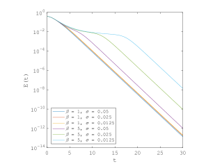
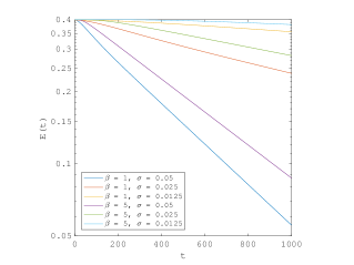
Figure 5.1: $E(t)$ for the nonlinear dynamics (3.1) (left) and continuum Metropolis dynamics (3.2) (right), for several different values of $\beta,\sigma$. Note the different horizontal and vertical axis scales at left and right.

Observe that within both schemes we observe linear convergence of the form

$$E(t)=Ce^{-t/\alpha}.$$

Note that $\alpha$ does not depend noticeably on $\beta,\sigma$ for the nonlinear dynamics (3.1) (and in fact is numerically close to $1$, consistent with Theorem 2). Meanwhile, as expected, $\alpha$ depends dramatically on $\beta,\sigma$ for the continuum Metropolis dynamics (3.2).

For the nonlinear dynamics when $\beta$ is large and $\sigma$ is small, we observe transient behavior before the asymptotic convergence regime. This corresponds to the regime in which the effective support of $\rho$ expands to match that of $\pi$, at which point rapid convergence ensues. This interpretation is visualized in Figure 5.2.

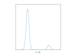
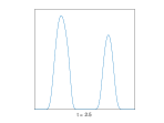
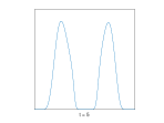
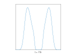
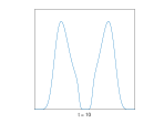
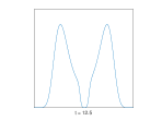
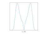
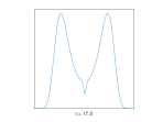
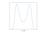
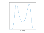
Figure 5.2: $\rho_{t}$ according to the nonlinear dynamics (3.1) with $\beta=5$, $\sigma=0.0125$ at times $t=0,\,2.5,\,5,\,7.5,\,10,\,12.5,\,15,\,17.5,\,20\,,22.5$, ordered left-to-right, then bottom-to-top. The profile at the last frame ($t=22.5$) is visually indistinguishable from that of $\pi$. The interval of the horizontal axis is fixed as $[-1.5,1.5]$ in all figures, but the interval of the vertical axis varies to accommodate the changing vertical scale.

Observe that even in the pre-asymptotic regime, the dynamics are able to achieve approximate balance between the probabilities of the two modes. This behavior (which may be viewed as arising from the nonlocal walker moves in the underlying ensemble scheme) contrasts sharply with that of the continuum Metropolis dynamics (3.2) for the same problem, visualized in Figure 5.3. Those dynamics can be viewed as locally ‘bulldozing’ probability from left to right, and in fact the height of the second mode initially decreases.

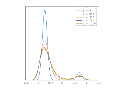
Figure 5.3: $\rho_{t}$ according to the continuum Metropolis dynamics (3.2) with $\beta=5$, $\sigma=0.0125$ at several different times. Note that even by time $t=1000$, the dynamics are far from convergence, and the height of the second mode has actually decreased relative to the initial condition.

5.2 Gaussian progress regression with Bayesian hyperparameters

In this section we consider the application of our method to Bayesian inference of hyperparameters in Gaussian process regression. For consistency with the application, the variable names in this section are not consistent with the choices made for the general setting considered above. The example problems are adapted from one considered in [31], which is also concerned with sampling for multimodal distributions.

In our experiments, we assess the efficiency of our methods in terms of integrated autocorrelation times (IAT) [28]. We are especially interested in the dependence of the efficiency on the number $N$ of walkers, with the case $N=1$ corresponding to an ordinary chain.

Specifically, we compute the average of one of the hyperparameters over the ensemble of walkers at each time to produce a time series. We define one step to be a move of a single walker. For an ensemble of $N$ walkers, we multiply the IAT of the aforementioned time series (estimated via the emcee software package [10]) by a factor of $1/N$. This allows for a fair comparison between different ensemble sizes. To see this, consider an ensemble scheme with $N$ walkers which do not interact. The dynamics should be identical to $N$ independent chains, each with a single walker. Since one step is defined by a move of one walker, we will need $N$ steps to move each independent chain once. Thus, dividing the IAT by $N$ makes the result consistent with that of a single chain. Note, moreover, that in an efficient implementation, the computational cost of our method (as measured by the number of calls to the likelihood function) with $N$ interacting walkers is equivalent to the cost of running $N$ non-interacting chains. For more on measuring convergence of ensemble schemes see [14].

5.2.1 Univariate case

First we consider a univariate mean-zero Gaussian process $\mathcal{GP}\left(0,\Sigma\right)$; see Appendix E for relevant background. We take the covariance to be

$$\Sigma(x_{1},x_{2})=\alpha^{2}\exp\left(-\frac{(x_{1}-x_{2})^{2}}{\rho^{2}}\right),$$

where $\alpha$ and $\rho$ are parameters (that we want to infer). These parameters, if known, specify our prior distribution $\mathcal{GP}\left(0,\Sigma\right)$ for an unknown function $f$.

Let us also assume that we are given several $x_{i}$, $i=1,\ldots,m$ and that we have observed the function values at these points, corrupted by some Gaussian noise, i.e., we have observed the data

$$y_{i}=f(x_{i})+\epsilon_{i},$$

where $\epsilon_{i}\sim\mathcal{N}(0,\sigma^{2})$. Here $\sigma$ is another model parameter that we wish to infer.

Let us collect our parameters as $\theta=(\alpha,\rho,\sigma)$ and set $f_{\mathbf{x}}=(f(x_{1}),\dots,f(x_{m}))$. Fix $K_{\theta}:=K(\mathbf{x},\mathbf{x})$, defined as in Appendix E, where here the subscript indicates the dependence of $K$ on $\theta$. Then note that

$$y=f_{\mathbf{x}}+\epsilon$$

is a sum of independent Gaussians with distributions $\mathcal{N}(0,K)$ and $\mathcal{N}(0,\sigma^{2}I)$. Hence $y$ is distributed as $\mathcal{N}(0,K+\sigma^{2}I)$.

Let $p(\theta)$ denote our prior for $\theta$. We seek to sample $\theta$ according to

$$p(\theta\,|\,y)\propto p(y\,|\,\theta)p(\theta)\propto|K_{\theta}+\sigma^{2}I|^{-1/2}\,e^{-\frac{1}{2}y^{\top}\left(K_{\theta}+\sigma^{2}I\right)^{-1}y}\,p(\theta),$$

where $y$ is fixed throughout.

For our experiments, we choose independent $\mathrm{Cauchy}^{+}(0,3)$ priors for $\theta=(\alpha,\rho,\sigma)$. Moreover we generate data $\mathbf{x}$ according to $x_{i}\sim\mathcal{N}(0,1)$ and $y$ according to $y_{i}=f_{\mathrm{true}}(x_{i})+\delta_{i}$, where

(5.1) $$f_{\mathrm{true}}(x_{i})=0.3+0.4x_{i}+0.5\sin(2.7x_{i})+1.1/(1+x_{i}^{2})$$

and

(5.2) $$\delta_{i}\sim\begin{cases}\mathcal{N}(0,0.125^{2})&|x_{i}|<1.5\\ \mathcal{N}(0,1.25^{2})&\text{otherwise}.\end{cases}$$

We sample from $p(\theta\,|\,y)$ using the ensemble method of Section 2, where the proposal $q(\,\cdot\,|\theta)$ is $\mathcal{N}(\theta,\beta^{2}I)$, $\beta^{2}=0.01$. In Figure 5.4, we plot posterior marginal distributions estimated from samples and compare against a ground truth obtained via numerical quadrature, which is feasible since $\theta$ is only 3-dimensional. Notice the multimodality of these marginals, suggesting the possibility of an advantage for the interacting walker scheme. In Table 1, we record estimated IATs for different ensemble sizes $N$, confirming the advantage of taking $N\gg 1$. In Figure 5.5, we plot the empirical acceptance probability $A$ and empirical teleport probability $T$ as functions of $N$. (The teleport probability is the probability that the indices of the cloned and removed walkers are different.)

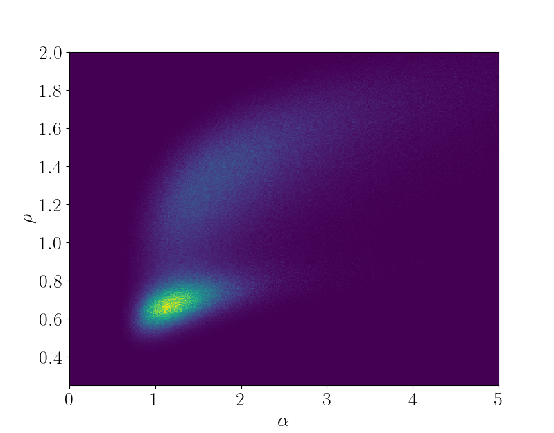
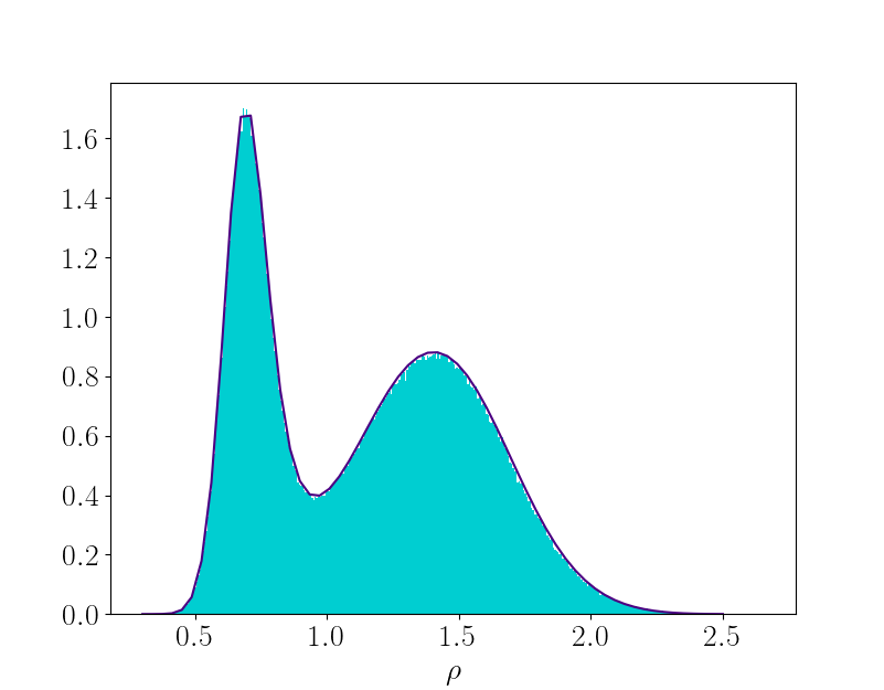
Figure 5.4: Univariate case. Posterior marginal distribution of $\alpha$ and $\rho$ (left) and numerically integrated density compared with sampled posterior of $\rho$ (right), obtained with ensemble size $N=50$.

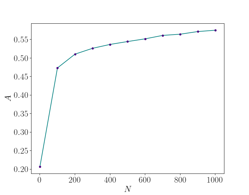
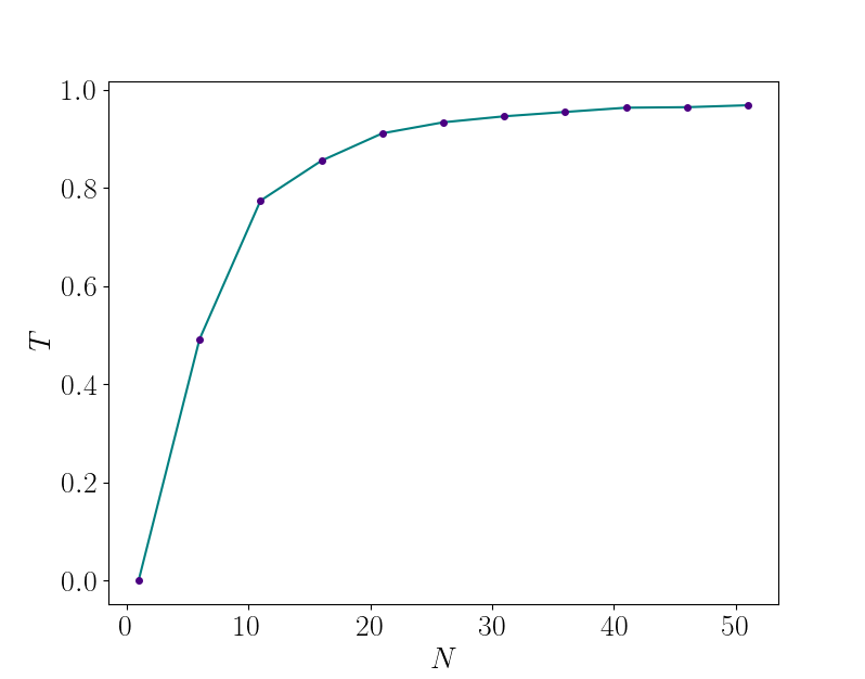
Figure 5.5: Univariate case. The acceptance probability $A$ versus $N$ (left) and the teleport probability $T$ versus $N$ (right), where $N$ is the number of walkers.

$N$	1	10	50
IAT	2111	857	97

Table 1: Univariate case. Integrated autocorrelation times of the average of $\rho$ over all walkers.

5.2.2 Multivariate case

Next we consider the case of a multivariate Gaussian process prior $\mathcal{GP}\left(0,\Sigma\right)$, where we take

$$\Sigma(x_{1},x_{2})=\alpha^{2}\exp\left(-(x_{1}-x_{2})^{\top}ZZ^{\top}(x_{1}-x_{2})\right).$$

Here $\alpha\in\mathbb{R}$ and $Z\in\mathbb{R}^{n\times n}$ (upper triangular) are parameters that we want to infer. Accordingly we collect our hyperparameters as $\theta=(\alpha,Z,\sigma)$. We maintain the same priors on $\alpha$ and $\sigma$, but we must specify a special prior for the upper triangular hyperparameter $Z$.

We want to choose a prior for $Z$ such that $ZZ^{\top}$ is distributed according to $W_{n}(I_{n},n)$, which is the Wishart distribution [2] with $n$ degrees of freedom and scale matrix $I_{n}$. Following the Bartlett decomposition [2], $Z$ is sampled as

$$Z=\left(\begin{array}[]{cccc}c_{1}&0&\cdots&0\\ z_{21}&c_{2}&\cdots&0\\ \vdots&\vdots&\ddots&\vdots\\ z_{n1}&z_{n2}&\cdots&c_{n}\end{array}\right),$$

where the entries are all independently distributed, $z_{ij}\sim\mathcal{N}(0,1)$ for all $i>j$, and $c_{i}$ is distributed according to the chi distribution with $n-i+1$ degrees of freedom.

We generate data $\mathbf{x}$ according to $x_{i}\sim\mathcal{N}(0,I_{n})$ and $y$ according to $y_{i}=f_{\mathrm{true}}(x_{i})+\delta_{i}$, where

$$f_{\mathrm{true}}(x_{i})=\prod_{j=1}^{n}\left(0.3+0.4x_{ij}+0.5\sin(2.7x_{ij})+1.1/(1+x_{ij}^{2})\right)$$

and $\delta_{i}=\sum_{j=1}^{n}\delta_{ij}$, where

$$\delta_{ij}\sim\begin{cases}\mathcal{N}(0,0.125^{2})&|x_{ij}|<1.5\\ \mathcal{N}(0,1.25^{2})&\text{otherwise}.\end{cases}$$

For our experiment we fix $n=3$.

Again we sample from $p(\theta\,|\,y)$ using the ensemble method of Section 2, where the proposal $q(\,\cdot\,|\theta)$ is $\mathcal{N}(\theta,D)$,

$$D=\left(\begin{array}[]{ccc}0.1&0&0\\ 0&0.01&0\\ 0&0&0.01\end{array}\right).$$

In Figures 5.6 and 5.7, we plot posterior marginal distributions estimated from samples, though now validation via numerical quadrature is not feasible due to the increased dimension of $\theta$. Again we observe multimodality, and Table 2 demonstrates improved efficiency for large ensemble sizes $N$.

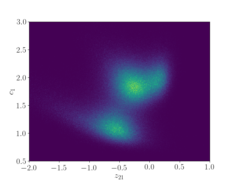
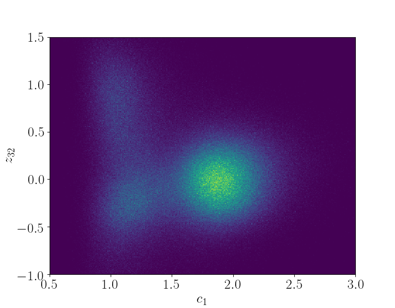
Figure 5.6: Multivariate case, $n=3$. Posterior marginal distribution of $z_{21}$ and $c_{1}$ (left) and of $c_{1}$ and $z_{32}$ (right), obtained with ensemble size $N=100$.

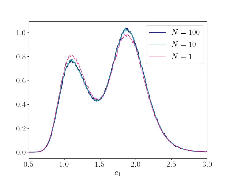
Figure 5.7: Multivariate case, $n=3$. Sampled posterior marginal distribution of $c_{1}$, obtained with ensemble sizes $N=1$, $10$, and $100$ and $10^{7}$ time steps. For $N>1$, only one walker (specifically, the one that was cloned) was entered into the histogram per step, so using the same number of time steps for each ensemble size is a fair comparison. Note the visible discrepancy for $N=1$ due to a long autocorrelation time.

$N$	1	10	20	50	100
IAT	1309	461	292	145	81

Table 2: Multivariate case, $n=3$. Integrated autocorrelation times of the average of $c_{1}$ over all walkers.

5.2.3 Non-Gaussian noise model

Finally we return to the univariate case but consider a non-Gaussian noise model for the $\epsilon_{i}$. Note that in this general case, we cannot explicitly ‘integrate out’ the $\epsilon_{i}$ as above, and we are forced to think of them as additional Bayesian parameters to be sampled. Then we must consider an expanded prior $p(\theta,\epsilon)=p(\theta)g_{\theta}(\epsilon)$, where $g_{\theta}$ denotes our non-Gaussian noise model, which may itself depend on the hyperparameters $\theta$. Then we want to sample $\theta,\epsilon$ according to

$$p(\theta,\epsilon\,|\,y)\propto p(y\,|\,\theta,\epsilon)p(\theta)g_{\theta}(\epsilon)\propto|K_{\theta}|^{-1/2}\,e^{-\frac{1}{2}(y-\epsilon)^{\top}K_{\theta}^{-1}(y-\epsilon)}\,p(\theta)\,g_{\theta}(\epsilon),$$

where $y$ is fixed throughout. Since $K_{\theta}$ is usually numerically low-rank, this expression is not suitable for sampling. We consider the change of variable $(\theta,\epsilon)\rightarrow(\theta,w)$ defined by $\epsilon=y+K_{\theta}^{1/2}w$, motivating us to sample $\theta,w$ according to

$$p(\theta,w\,|\,y)\propto e^{-\frac{1}{2}\|w\|^{2}}\,p(\theta)\,g_{\theta}(\epsilon).$$

We take the same prior $p(\theta)$ for $\theta=(\alpha,\rho,\sigma)$ as above, and for our noise prior we consider independent Student-$t$ distributions for each $\epsilon_{i}$, each with mean $0$, scale $\sigma$ (a hyperparameter), and $\nu=2$ degrees of freedom.

We generate data $\mathbf{x}$ according to $x_{i}\sim\mathcal{N}(0,1)$ and $y$ according to $y_{i}=f_{\mathrm{true}}(x_{i})+\delta_{i}$, where $f_{\mathrm{true}}$ and $\delta_{i}$ are the same as in (5.1) and (5.2).

We sample from $p(\theta,w\,|\,y)$ using the method of Section 4, employing walker interaction only for the $\theta$ variables. The proposals $q(\,\cdot\,|\theta)$ and $r(\,\cdot\,|w)$ are distributed according to $\mathcal{N}(\theta,D)$ and $\mathcal{N}(w,\beta^{2}I)$, respectively, where

$$D=\left(\begin{array}[]{ccc}0.001&0&0\\ 0&0.001&0\\ 0&0&0.0001\end{array}\right)$$

and $\beta^{2}=0.001$. We run the parallel chains for the $w$ variables for $30$ steps between each update step for the interacting $\theta$ variables. In Figure 5.7, we plot a posterior marginal distribution estimated from samples. Notice that, relative to Figure 5.4, the previously observed multimodality vanishes for this noise model. Nonetheless, we still see an advantage for large ensembles in Table 3.

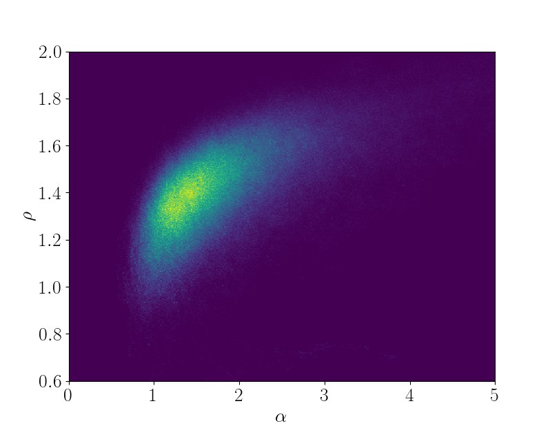
Figure 5.8: Non-Gaussian noise model. Posterior distribution of $\alpha$ and $\rho$, obtained with ensemble size $N=60$. Note that with the Student-$t$ noise model, we lose the multimodality in $\rho$.

$N$	1	20	40	60
IAT	26016	20453	12428	6090

Table 3: Non-Gaussian noise model. Integrated autocorrelation times of the average of $\rho$ over all walkers.

Appendix A Acceptance probability computations

Observe that the likelihood $Q(\mathbf{x}^{\prime}\,|\,\mathbf{x})$ of the proposal of Section 2 is given by

$$Q(\mathbf{x}^{\prime}\,|\,\mathbf{x})=\begin{cases}w_{i}(\mathbf{x},x_{i}^{\prime})\frac{1}{N}\sum_{k=1}^{N}q(x_{i}^{\prime}|x_{k}),&\mbox{if $\mathbf{x}^{\prime}$ and $\mathbf{x}$ differ on a unique index $i$,}\\ 0,&\mbox{otherwise}.\end{cases}$$

Supposing that we have generated $\mathbf{x^{\prime}}$ via the procedure described in Section 2 (i.e., so that $i$, $j$, and $z$ are defined as above), the Metropolis-Hastings acceptance probability is given by

$$A = \min\left(1,\frac{\Pi(\mathbf{x}^{\prime})}{\Pi(\mathbf{x})}\frac{Q(\mathbf{x}\,|\,\mathbf{x}^{\prime})}{Q(\mathbf{x}^{\prime}\,|\,\mathbf{x})}\right)$$

$$= \min\left(1,\frac{\pi(z)}{\pi(x_{i})}\frac{w_{i}(\mathbf{x}^{\prime},x_{i})}{w_{i}(\mathbf{x},z)}\frac{\sum_{k=1}^{N}q(x_{i}|x_{k}^{\prime})}{\sum_{k=1}^{N}q(z|x_{k})}\right)$$

$$= \min\left(1,\frac{\pi(z)}{\pi(x_{i})}\frac{Z(\mathbf{x},z)}{Z(\mathbf{x}^{\prime},x_{i})}\frac{\left(\frac{q(x_{i}^{\prime}\,|\,x_{i})+\sum_{k\neq i}^{N}q(x_{i}^{\prime}\,|\,x_{k}^{\prime})}{\pi(x_{i}^{\prime})}\right)}{\left(\frac{q(x_{i}\,|\,z)+\sum_{k\neq i}^{N}q(x_{i}\,|\,x_{k})}{\pi(x_{i})}\right)}\frac{\sum_{k=1}^{N}q(x_{i}\,|\,x_{k}^{\prime})}{\sum_{k=1}^{N}q(z\,|\,x_{k})}\right).$$

But recall $x_{i}^{\prime}=z$, and $x_{k}^{\prime}=x_{k}$ for $k\neq i$, so

$$A = \min\left(1,\frac{Z(\mathbf{x},z)}{Z(\mathbf{x}^{\prime},x_{i})}\frac{q(z\,|\,x_{i})+\sum_{k\neq i}^{N}q(z\,|\,x_{k})}{q(x_{i}\,|\,z)+\sum_{k\neq i}^{N}q(x_{i}\,|\,x_{k})}\frac{\sum_{k=1}^{N}q(x_{i}|x_{k}^{\prime})}{\sum_{k=1}^{N}q(z|x_{k})}\right)$$

$$= \min\left(1,\frac{Z(\mathbf{x},z)}{Z(\mathbf{x}^{\prime},x_{i})}\frac{\sum_{k=1}^{N}q(z\,|\,x_{k})}{\sum_{k=1}^{N}q(x_{i}\,|\,x_{k}^{\prime})}\frac{\sum_{k=1}^{N}q(x_{i}\,|\,x_{k}^{\prime})}{\sum_{k=1}^{N}q(z\,|\,x_{k})}\right)$$

$$= \min\left(1,\frac{Z(\mathbf{x},z)}{Z(\mathbf{x}^{\prime},x_{i})}\right),$$

as desired.

Appendix B Global convergence proof

Proof.

For consistency of presentation, we will maintain the continuous notation, i.e., writing integrals over $X$ instead of sums.

From the dynamics (3.1) we have

$$\dot{\rho}=\mathcal{Q}\rho-Z_{\rho}^{-1}\frac{\mathcal{Q}\rho}{\pi}\rho=:G[\rho].$$

Note that $G[\rho](x)>0$ if $\rho(x)=0$ because $\mathcal{Q}\rho$ has full support. By the continuity of $G$ and the compactness of the space of probability measures, for any $x$, we have $\dot{\rho}(x)=G[\rho](x)>0$ if $\rho(x)<\delta$ for some $\delta>0$ sufficiently small. Consequently $\mathrm{supp}(\rho_{t})=X$ for all $t>0$ at which $\rho_{t}$ is defined (even if $\mathrm{supp}(\rho_{0})\neq X$). Moreover, as the constraint that $\int\rho\,dx=1$ is conserved by the dynamics (3.1), we also have that $\rho_{t}$ lies within the probability simplex for all times $t$ at which it is defined. This a priori bound within a compact region, together with a Lipschitz condition on the dynamics within this domain, guarantees global-in-time existence of $\rho_{t}$ by standard theory (cf., [29]).

Recall (3.3), i.e., that

$$\frac{d}{dt}\chi^{2}(\pi\,\|\,\rho_{t})\leq-\mathrm{Var}_{\mathcal{Q}\rho}(\pi/\rho_{t}),$$

Define the sublevel set

$$S_{b}:=\left\{\rho\ \mathrm{prob.\,dens.}\,:\,\chi^{2}(\pi\,\|\,\rho)\leq b\right\},$$

and note by monotonicity that setting $b=\chi^{2}(\pi\,\|\,\rho_{0})$, we have $\rho_{t}\in S_{b}$ for all $t$. Then evidently

$$\frac{d}{dt}\chi^{2}(\pi\,\|\,\rho_{t})\leq-\mathrm{Var}_{\rho}(\pi/\rho_{t})\inf_{\rho\in S_{b}}\left\{\frac{\mathrm{Var}_{\mathcal{Q}\rho}(\pi/\rho)}{\mathrm{Var}_{\rho}(\pi/\rho)}\right\}=-\gamma^{-1}\,\chi^{2}(\pi\,\|\,\rho_{t}),$$

where $\alpha$ is defined as in the statement of the theorem. Then (3.4) follows from Grönwall’s inequality, provided we can show that $\gamma<+\infty$. Note that $\gamma<+\infty$ holds if we can show (3.5), so remains only to show (3.5).

Now

$$\mathrm{Var}_{\mathcal{Q}\rho}\left[\pi/\rho\right] = \int\left[\frac{\pi}{\rho}-\left(\int\frac{\pi}{\rho}\,\mathcal{Q}\rho\,dx\right)\right]^{2}\,\mathcal{Q}\rho\,dx$$

$$\geq \|\rho/\mathcal{Q}\rho\|_{\infty}^{-1}\int\left[\frac{\pi}{\rho}-\left(\int\frac{\pi}{\rho}\,\mathcal{Q}\rho\,dx\right)\right]^{2}\,\rho\,dx.$$

But note that $\int\left(\frac{\pi}{\rho}-a\right)^{2}\rho\,dx$ is minimized over $a\in\mathbb{R}$ by taking $a=\int\frac{\pi}{\rho}\,\rho\,dx=1$, so

$$\int\left[\frac{\pi}{\rho}-\left(\int\frac{\pi}{\rho}\,\mathcal{Q}\rho\,dx\right)\right]^{2}\,\rho\,dx\geq\mathrm{Var}_{\rho}(\pi/\rho).$$

Hence $\mathrm{Var}_{\mathcal{Q}\rho}\left[\pi/\rho\right]\geq\|\rho/\mathcal{Q}\rho\|_{\infty}^{-1}\mathrm{Var}_{\rho}(\pi/\rho)$, which implies (3.5).

Appendix C Linearization computations and asymptotic convergence proof

Let

$$F(\eta)=\frac{1}{Z_{\pi+\eta}}\left[Z_{\pi+\eta}-\frac{\pi+\eta}{\pi}\right]\mathcal{Q}(\pi+\eta)$$

as Section 3.2. Recall that $Z_{\rho}=\int\frac{\rho\mathcal{Q}\rho}{\pi}\,dx$. In particular $Z_{\pi}=1$. We want to compute $DF(0)$. Now in our expression for $F(\eta)$, the middle factor is zero when $\eta=0$, hence in the product rule only one term contributes and we have

$$\frac{\delta F(\eta)(x)}{\delta\eta(y)}\bigg{|}_{\eta=0} = \mathcal{Q}\pi(x)\frac{\delta}{\delta\eta(y)}\bigg{|}_{\eta=0}\left[Z_{\pi+\eta}-\frac{\pi(x)+\eta(x)}{\pi(x)}\right]$$

$$= \mathcal{Q}\pi(x)\left[\frac{\delta}{\delta\eta(y)}\bigg{|}_{\eta=0}Z_{\pi+\eta}-\frac{\delta(x,y)}{\pi(x)}\right].$$

To deal with the partition function, observe that

$$Z_{\rho}=\rho^{*}\left[\mathrm{diag}(\pi)^{-1}\mathcal{Q}\right]\rho=\frac{1}{2}\rho^{*}\left[\mathrm{diag}(\pi)^{-1}\mathcal{Q}+\mathcal{Q}^{*}\mathrm{diag}(\pi)^{-1}\right]\rho,$$

i.e., we may view $Z_{\rho}$ as a symmetric quadratic form in $\rho$. Hence

$$\frac{\delta}{\delta\rho}Z_{\rho}=\left(\mathrm{diag}(\pi)^{-1}\mathcal{Q}+\mathcal{Q}^{*}\mathrm{diag}(\pi)^{-1}\right)\rho=\frac{\mathcal{Q}\rho}{\pi}+\mathcal{Q}^{*}\left(\frac{\rho}{\pi}\right).$$

But then

$$\frac{\delta}{\delta\eta(y)}\bigg{|}_{\eta=0}Z_{\pi+\eta}=\frac{\delta}{\delta\rho(y)}\bigg{|}_{\rho=\pi}Z_{\rho}=\frac{\mathcal{Q}\pi}{\pi}(y)+[\mathcal{Q}^{*}\mathbf{1}](y)=\frac{\mathcal{Q}\pi}{\pi}(y)+1,$$

where $\mathbf{1}$ is the constant function taking value $1$, and we used that $\mathcal{Q}^{*}\mathbf{1}=1$ because $\mathcal{Q}$ is a Markov transition operator.

In summary we have established that

$$\mathcal{J}(x,y):=\frac{\delta F(\eta)(x)}{\delta\eta(y)}\bigg{|}_{\eta=0}=\mathcal{Q}\pi(x)\left[\frac{\mathcal{Q}\pi}{\pi}(y)+1-\frac{\delta(x,y)}{\pi(x)}\right],$$

where $\mathcal{J}(x,y)$ denotes the kernel of the operator $DF(0)$. Then

$$\mathcal{J}=\mathcal{Q}\pi\left(\frac{\mathcal{Q}\pi}{\pi}\right)^{*}-\mathrm{diag}\left(\frac{\mathcal{Q}\pi}{\pi}\right)+\left(\mathcal{Q}\pi\right)\mathbf{1}^{*}.$$

But since $\mathbf{1}^{*}\eta=0$ for all $\eta\in S$, we have that

$$\mathcal{J}=\mathcal{Q}\pi\left(\frac{\mathcal{Q}\pi}{\pi}\right)^{*}-\mathrm{diag}\left(\frac{\mathcal{Q}\pi}{\pi}\right)$$

as an operator on $S$ (and indeed one verifies easily $S$ is invariant under $\mathcal{J}$ so defined).

Proof of Theorem 2.

For consistency of presentation, we maintain the continuous notation, i.e., writing integrals over $X$ instead of sums. In the finite-dimensional case, the computation of the Jacobian $DF(0)$ for the dynamics $\dot{\eta}=F(\eta)$ in Appendix C is rigorous without further clarification. Then standard stable manifold theory for ODEs (cf., Theorem 9.4 of [29]) guarantees the result, provided we can show that $\sigma(\mathcal{J})\subset\mathbb{R}$ with $\sup\sigma(\mathcal{J})<-\|\pi/\mathcal{Q}\pi\|_{\infty}^{-1}$.

First note that taking $\mathcal{D}:=\mathrm{diag}(\sqrt{\pi})$ we have

$$\mathcal{M}:=\mathcal{D}^{-1}\mathcal{J}\mathcal{D}=\left(\frac{\mathcal{Q}\pi}{\sqrt{\pi}}\right)\left(\frac{\mathcal{Q}\pi}{\sqrt{\pi}}\right)^{*}-\mathrm{diag}\left(\frac{\mathcal{Q}\pi}{\pi}\right).$$

Then $\mathcal{M}$ is self-adjoint, hence diagonalizable with real eigenvalues. Since $\mathcal{M}$ and $\mathcal{J}$ are similar, $\mathcal{J}$ is also diagonalizable with the same eigenvalues. Note that $\mathcal{M}$ is on operator on $\mathcal{D}^{-1}S=\{f\,:\,\int f\sqrt{\pi}\,dx=0\}$, not on $S$.

To complete the proof it then suffices to show that $f^{*}\mathcal{M}f<-\|\pi/\mathcal{Q}\pi\|_{\infty}^{-1}\,f^{*}f$ for any $f$ with $\int f\sqrt{\pi}\,dx=0$. Observe that

(C.1) $$f^{*}\mathcal{M}f=\left(\int\frac{\mathcal{Q}\pi}{\sqrt{\pi}}f\,dx\right)^{2}-\int\frac{\mathcal{Q}\pi}{\pi}f^{2}\,dx.$$

Since $\int f\sqrt{\pi}\,dx=0$, we may write, for an arbitrary constant $c$ (to be optimized later):

$$\left(\int\frac{\mathcal{Q}\pi}{\sqrt{\pi}}f\,dx\right)^{2} = \left(\int\frac{\mathcal{Q}\pi-c\pi}{\sqrt{\pi}}f\,dx\right)^{2}$$

$$= \left(\int\sqrt{\mathcal{Q}\pi}\,\frac{\sqrt{\mathcal{Q}\pi}-c\frac{\pi}{\sqrt{\mathcal{Q}\pi}}}{\sqrt{\pi}}f\,dx\right)^{2}$$

$$\leq \left[\int\mathcal{Q}\pi\,dx\right]\left[\int\left(\sqrt{\mathcal{Q}\pi}-c\frac{\pi}{\sqrt{\mathcal{Q}\pi}}\right)^{2}\frac{f^{2}}{\pi}\,dx\right],$$

where the inequality follows from the Cauchy-Schwarz inequality. But $\int\mathcal{Q}\pi\,dx=1$, and expanding the square in the other integrand yields

$$\left(\int\frac{\mathcal{Q}\pi}{\sqrt{\pi}}f\,dx\right)^{2}\leq\int\frac{\mathcal{Q}\pi}{\pi}f^{2}\,dx-2c\int f^{2}\,dx+c^{2}\int\frac{\pi}{\mathcal{Q}\pi}f^{2}\,dx.$$

By plugging into (C.1) we see that

$$f^{*}\mathcal{M}f\leq-2c\int f^{2}\,dx+c^{2}\int\frac{\pi}{\mathcal{Q}\pi}f^{2}\,dx.$$

Then we want to optimize this bound over $c$. Evidently the optimal $c$ is given by

$$c=\frac{\int f^{2}\,dx}{\int\frac{\pi}{\mathcal{Q}\pi}f^{2}\,dx},$$

which yields

$$f^{*}\mathcal{M}f\leq-\frac{(f^{*}f)^{2}}{\int\frac{\pi}{\mathcal{Q}\pi}f^{2}\,dx}.$$

But $\int\frac{\pi}{\mathcal{Q}\pi}f^{2}\,dx\leq\|\pi/\mathcal{Q}\pi\|_{\infty}\,f^{*}f$, so $f^{*}\mathcal{M}f\leq-\|\pi/\mathcal{Q}\pi\|_{\infty}^{-1}\,f^{*}f$, as was to be shown.

Appendix D Gradient flow computations

Expanding the expression in (3.7) to lowest order we obtain the asymptotically equivalent problem:

$$\rho_{\varepsilon}=\underset{\tilde{\rho}\in\mathcal{P}(X)}{\mbox{argmin}}\left\{\int\frac{\delta E(\rho)}{\delta\rho(x)}\,(\tilde{\rho}(x)-\rho(x))\ dx+\frac{1}{8\varepsilon}\int\frac{(\tilde{\rho}(x)-\rho(x))^{2}}{\rho(x)}\ dx\right\}.$$

Now

$$\frac{\delta}{\delta\rho(x)}E(\rho)=\frac{1}{8}\frac{\delta}{\delta\rho(x)}\int\left(1-\frac{\rho}{\pi}\right)^{2}\pi\,dx=\frac{1}{4}\left(\frac{\rho(x)}{\pi(x)}-1\right),$$

so we must solve

$$\underset{\tilde{\rho}\in\mathcal{P}(X)}{\mbox{argmin}}\left\{\frac{1}{4}\int\left(\frac{\rho}{\pi}-1\right)(\tilde{\rho}-\rho)\ dx+\frac{1}{8\varepsilon}\int\frac{(\tilde{\rho}-\rho)^{2}}{\rho}\ dx\right\}.$$

for which the optimality condition is

$$1-\frac{\rho}{\pi}=\frac{1}{\varepsilon}\frac{\tilde{\rho}-\rho}{\rho}-\lambda,$$

where $\lambda$ is a constant, namely the Lagrange multiplier for the constraint $\int\rho\,dx=1$. Rearranging we obtain

$$\rho_{\varepsilon}=\rho+\varepsilon\left[\left(1-\frac{\rho}{\pi}\right)\rho+\lambda\rho\right],$$

where $\lambda$ is chosen so that $\int\rho_{\varepsilon}=1$. Notice that this means precisely that $\lambda=C_{p}$, hence we obtain

$$\partial_{\tau}\rho=\left(1-\frac{\rho}{\pi}\right)\rho+C_{\rho}\,\rho,$$

as desired.

Appendix E Gaussian processes

A Gaussian process is a random function $f:\mathbb{R}^{n}\rightarrow\mathbb{R}$ specified by a mean $\mu(x)$ and covariance $\Sigma(x_{1},x_{2})$ which satisfy

$$\mathbb{E}\left[f(x)\right]=\mu(x)$$

and

$$\mathbb{E}\left[\left(f(x_{1})-\mu(x_{2})\right)\left(f(x_{1})-\mu(x_{2})\right)\right]=\Sigma(x_{1},x_{2}),$$

together with the specification that for any choice of $\mathbf{x}=(x_{1},\ldots,x_{m})\in\mathbb{R}^{n\times m}$, the random vector

$$f_{\mathbf{x}}:=(f(x_{1}),\ldots,f(x_{n}))$$

is Gaussian distributed. Hence note that in particular $f_{\mathbf{x}}$ has mean

$$\left(\mu(x_{1}),\ldots,\mu(x_{n})\right)$$

and covariance

$$K(\mathbf{x},\mathbf{x}):=\left(\begin{array}[]{ccc}\Sigma(x_{1},x_{1})&\cdots&\Sigma(x_{1},x_{n})\\ \vdots&\ddots&\vdots\\ \Sigma(x_{n},x_{1})&\cdots&\Sigma(x_{n},x_{n})\end{array}\right).$$

In this case we say that $f\sim\mathcal{GP}\left(\mu,\Sigma\right)$.

References

- [1] L. Ambrosio, N. Gigli, and G. Savaré, Gradient Flows in Metric Spaces and in the Space of Probability Measures, Birkhäuser Verlag, 2005.
- [2] T. W. Anderson, An Introduction to Multivariate Statistical Analysis, Wiley Interscience, 2003.
- [3] C. Andrieu, A. Jasra, A. Doucet, and P. Del Moral, Non-linear Markov chain Monte Carlo, in Conference Oxford sur les méthodes de Monte Carlo séquentielles, vol. 19 of ESAIM Proc., EDP Sci., Les Ulis, 2007, pp. 79–84, https://doi.org/10.1051/proc:071911, https://doi.org/10.1051/proc:071911.
- [4] C. J. T. Braak, A Markov chain Monte Carlo version of the genetic algorithm differential evolution: easy Bayesian computing for real parameter spaces, Statistics and Computing, 16 (2006), pp. 239–249.
- [5] N. Chopin, T. Lelièvre, and G. Stoltz, Free energy methods for Bayesian inference: efficient exploration of univariate Gaussian mixture posteriors, Statistics and Computing, 22 (2012), pp. 897–916.
- [6] N. Chopin and O. Papaspiliopoulos, An Introduction to Sequential Monte Carlo, Springer Series in Statistics, Springer International Publishing, 2020.
- [7] J. A. Christen and C. Fox, A general purpose sampling algorithm for continuous distributions (the t-walk), Bayesian Analysis, 5 (2010), pp. 263–282.
- [8] A. R. Dinner, E. H. Thiede, B. V. Koten, and J. Weare, Stratification as a general variance reduction method for Markov chain Monte Carlo, SIAM/ASA Journal on Uncertainty Quantification, 8 (2020), pp. 1139–1188, https://doi.org/10.1137/18M122964X, https://arxiv.org/abs/https://doi.org/10.1137/18M122964X.
- [9] D. J. Earl and M. W. Deem, Parallel tempering: Theory, applications, and new perspectives, Phys. Chem. Chem. Phys., 7 (2005), pp. 3910–3916, https://doi.org/10.1039/B509983H, http://dx.doi.org/10.1039/B509983H.
- [10] D. Foreman-Mackey, D. W. Hogg, D. Lang, and J. Goodman, emcee: The MCMC Hammer. Preprint at https://arxiv.org/abs/1202.3665, 2013, https://doi.org/10.1086/670067, https://arxiv.org/abs/1202.3665. (accessed May 4, 2021).
- [11] A. Garbuno-Inigo, F. Hoffmann, W. Li, and A. M. Stuart, Interacting Langevin diffusions: gradient structure and ensemble Kalman sampler, SIAM J. Appl. Dyn. Syst., 19 (2020), pp. 412–441, https://doi.org/10.1137/19M1251655, https://doi.org/10.1137/19M1251655.
- [12] A. Garbuno-Inigo, N. Nüsken, and S. Reich, Affine invariant interacting Langevin dynamics for Bayesian inference, SIAM J. Appl. Dyn. Syst., 19 (2020), pp. 1633–1658, https://doi.org/10.1137/19M1304891, https://doi.org/10.1137/19M1304891.
- [13] W. R. Gilks, G. O. Roberts, and E. I. George, Adaptive direction sampling, Journal of the Royal Statistical Society. Series D (The Statistician), 43 (1994), pp. pp. 179–189, http://www.jstor.org/stable/2348942.
- [14] J. Goodman and J. Weare, Ensemble samplers with affine invariance, Communications in Applied Mathematic and Computational Science, 5 (2010), pp. 65–80.
- [15] P. Greengard, An ensemblized Metropolized Langevin sampler, master’s thesis, NYU, 2015.
- [16] B. Helffer, M. Klein, and F. Nier, Quantitative analysis of metastability in reversible diffusion processes via a Witten complex approach, Mat. Contemp., 26 (2004), pp. 41–85.
- [17] B. Leimkuhler and C. Matthews, Molecular dynamics, vol. 39 of Interdisciplinary Applied Mathematics, Springer, Cham, 2015. With deterministic and stochastic numerical methods.
- [18] B. Leimkuhler, C. Matthews, and J. Weare, Ensemble preconditioning for Markov chain Monte Carlo simulation, Stat. Comput., 28 (2018), pp. 277–290, https://doi.org/10.1007/s11222-017-9730-1, https://doi.org/10.1007/s11222-017-9730-1.
- [19] T. Lelièvre and G. Stoltz, Partial differential equations and stochastic methods in molecular dynamics, Acta Numer., 25 (2016), pp. 681–880, https://doi.org/10.1017/S0962492916000039, https://doi.org/10.1017/S0962492916000039.
- [20] D. A. Levin and Y. Peres, Markov chains and mixing times, American Mathematical Society, Providence, RI, 2017, https://doi.org/10.1090/mbk/107, https://doi.org/10.1090/mbk/107. Second edition of [ MR2466937], With contributions by Elizabeth L. Wilmer, With a chapter on “Coupling from the past” by James G. Propp and David B. Wilson.
- [21] F. Liese and I. Vajda, On divergences and informations in statistics and information theory, IEEE Trans. Inf. Theory, 52 (2006), pp. 4394 – 4412.
- [22] J. S. Liu, Monte Carlo strategies in scientific computing, Springer Series in Statistics, Springer-Verlag, New York, 2001.
- [23] Y. Lu, J. Lu, and J. Nolen, Accelerating Langevin sampling with birth-death, 2019, https://arxiv.org/abs/1905.09863.
- [24] C. Matthews, J. Weare, A. Kravtsov, and E. Jennings, Umbrella sampling: a powerful method to sample tails of distributions, Monthly Notices of the Royal Astronomical Society, 480 (2018), pp. 4069–4079, https://doi.org/10.1093/mnras/sty2140, https://doi.org/10.1093/mnras/sty2140, https://arxiv.org/abs/https://academic.oup.com/mnras/article-pdf/480/3/4069/25524203/sty2140.pdf.
- [25] G. A. Pavliotis, A. M. Stuart, and U. Vaes, Derivative-free bayesian inversion using multiscale dynamics, 2021, https://arxiv.org/abs/2102.00540.
- [26] J. Pidstrigach and S. Reich, Affine-invariant ensemble transform methods for logistic regression, 2021, https://arxiv.org/abs/2104.08061.
- [27] G. Rotskoff, S. Jelassi, J. Bruna, and E. Vanden-Eijnden, Global convergence of neuron birth-death dynamics, 2019, https://arxiv.org/abs/1902.01843.
- [28] A. Sokal, Monte Carlo Methods in Statistical Mechanics: Foundations and New Algorithms, Springer US, Boston, MA, 1997, pp. 131–192, https://doi.org/10.1007/978-1-4899-0319-8_6, https://doi.org/10.1007/978-1-4899-0319-8_6.
- [29] G. Teschl, Ordinary Differential Equations and Dynamical Systems, American Mathematical Society, 2012.
- [30] R. J. Webber, D. Aristoff, and G. Simpson, A splitting method to reduce mcmc variance, 2020, https://arxiv.org/abs/2011.13899.
- [31] Y. Yao, A. Vehtari, and A. Gelman, Stacking for non-mixing bayesian computations: The curse and blessing of multimodal posteriors, arXiv:2006.12335, (2020).
- [32] J. Zuntz, M. Paterno, E. Jennings, D. Rudd, A. Manzotti, S. Dodelson, S. Bridle, S. Sehrish, and J. Kowalkowski, CosmoSIS: Modular cosmological parameter estimation, Astronomy and Computing, 12 (2015), pp. 45–59, https://doi.org/10.1016/j.ascom.2015.05.005, https://arxiv.org/abs/1409.3409.