Multi-Objectivizing Software Configuration Tuning

Abstract.

Automatically tuning software configuration for optimizing a single performance attribute (e.g., minimizing latency) is not trivial, due to the nature of the configuration systems (e.g., complex landscape and expensive measurement). To deal with the problem, existing work has been focusing on developing various effective optimizers. However, a prominent issue that all these optimizers need to take care of is how to avoid the search being trapped in local optima — a hard nut to crack for software configuration tuning due to its rugged and sparse landscape, and neighboring configurations tending to behave very differently. Overcoming such in an expensive measurement setting is even more challenging. In this paper, we take a different perspective to tackle this issue. Instead of focusing on improving the optimizer, we work on the level of optimization model. We do this by proposing a meta multi-objectivization model (MMO) that considers an auxiliary performance objective (e.g., throughput in addition to latency). What makes this model unique is that we do not optimize the auxiliary performance objective, but rather use it to make similarly-performing while different configurations less comparable (i.e. Pareto nondominated to each other), thus preventing the search from being trapped in local optima.

Experiments on eight real-world software systems/environments with diverse performance attributes reveal that our MMO model is statistically more effective than state-of-the-art single-objective counterparts in overcoming local optima (up to 42% gain), while using as low as 24% of their measurements to achieve the same (or better) performance result.

1. Introduction

“All I want is to optimize the latency of my software; any other performance attributes are out of interest.”        (An anonymous industry partner)

The above quotation comes from one of our industry partners who is working in the finance sector, commenting on the need of tuning the configuration of a software system that manages all financial trading in his company. In this case, only a single performance attribute matter (i.e., latency) — in the finance sector, a millisecond decrease in the trade delay may boost a high-speed firm’s earnings by about 100 million USD per year (Tian et al., 2015).

Indeed, given the flexibility of highly-configurable software systems, automatically tuning their critical configuration options will affect a set of performance attributes, such as latency, throughput, and energy consumption (Shahbazian et al., 2020; Chen et al., 2018d; Nair et al., 2020; Chen et al., 2020, 2018b, 2018a). However, there are also many other cases, such as the above one, wherein only the optimization of a single performance attribute is of interest, whose minimization (or maximization) serves as the sole performance objective in consideration. In another scenario, machine learning systems deployed by large organizations (e.g., GPT-3 (Brown et al., 2020)), or those in the health care domain (Ahmad et al., 2018), often concern mainly on the accuracy, while caring little about the overhead/resources incurred for training. This has been well-echoed from the literature on software configuration tuning, in majority of which only a single performance attribute is considered at a time (Bergstra and Bengio, 2012; Ye and Kalyanaraman, 2003; Oh et al., 2017; Xi et al., 2004; Li et al., 2014; Behzad et al., 2013; Li et al., 2020c, b).

Despite only a single performance attribute is of concern, such an optimization scenario is not easy to deal with. This is because (1) the configurable systems involve a daunting number of configuration options with complex interactions, rendering a black-box to the software engineers (Xu et al., 2015; Chen, 2019; Chen and Bahsoon, 2017a); (2) the number of possible configurations to examine can be high (Chen and Bahsoon, 2017b) and the measurement of each configuration through running the software system is often expensive (Jamshidi and Casale, 2016); and (3) there is generally a high degree of sparsity in the configurable software systems (Nair et al., 2020), i.e., the close configurations can also have radically different performance. The last characteristic poses a particular challenge to any automatic tuning process in finding the optimal configuration (performance), because firstly different configurations may achieve locally good, but globally undesired performance (e.g., local optima); and secondly, the landscape of a (local) optimum’s neighborhood can be steep and rugged — if the tuning is trapped in a local optimum, it may be hard to escape from it as their neighboring configurations often perform worse than it. As an example, Figure 1 shows the projected configuration landscape for Apache Storm (2 out of 6 configuration options), where it can be clearly seen that even with this simplified version, the landscape is rather rugged and contains steep “local optimum traps”, resulting in significant difficulty in the tuning.

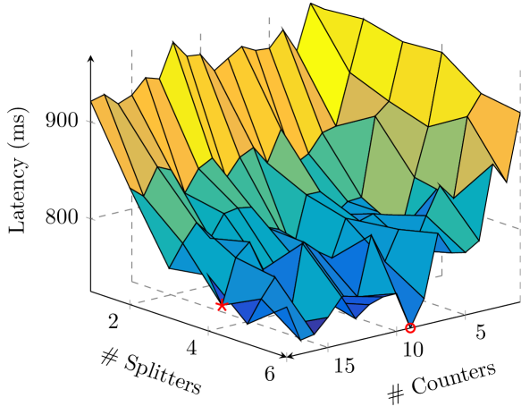
Figure 1. A projected landscape of the performance objective Latency with respect to configuration options Splitters and Counters for Storm under the WordCount benchmark.  is the global optimum and  is one of the locally optimal latency that an optimizer needs to escape from.

To address the above challenges, a number of optimizers from the Search-Based Software Engineering (SBSE) paradigm have been presented, such as random search (Bergstra and Bengio, 2012; Ye and Kalyanaraman, 2003; Oh et al., 2017), hill climbing (Xi et al., 2004; Li et al., 2014), genetic algorithm (Behzad et al., 2013; Shahbazian et al., 2020), and simulated annealing (Ding et al., 2015; Guo et al., 2010). To seek the global optimum (best performance of the concerned performance attribute) while avoiding being trapped in local optima, these methods focus on the “internal” components of the optimizer. They work on designing novel search operators (i.e., the way to change the configuration structure, for example, increasing the neighbourhood size of randomly mutated configurations (Oh et al., 2017)), or developing various search strategies (i.e., the way to balance exploration and exploitation, for example, restarting the search in hill climbing (Xi et al., 2004)). However, a major limitation of such single-objective optimizers is that the goal to find the global optimum is “less oriented” as there is no clear “incentive” to encourage them to traverse the wide search space and locating many local optima as possible, thus finding the best one in a resource-efficient manner.

In this paper, we look to tackle this software configuration tuning problem (with a single performance concern) from a different perspective. In contrast to the effort made by the existing works on the development of the optimizer, we work on the optimization model. We present a multi-objective optimization model for this single-objective problem, to help the search avoid being trapped in local optima and progressively explore the entire objective space — an approach that belongs to the concept called multi-objectivization (Knowles et al., 2001).

Multi-objectivization, which transforms a single-objective optimization problem into a multi-objective one, is not particularly unusual in SBSE. In several SE scenarios, researchers carefully design an auxiliary objective as a helper, along with the target objective (i.e., the original objective), for a multi-objective optimizer to deal with (Yuan and Banzhaf, 2020; Derakhshanfar et al., 2020; Mkaouer et al., 2014; Soltani et al., 2018). For example, in the crash reproduction problem (Derakhshanfar et al., 2020), a new auxiliary objective was created to check how widely a test case covers the code, which is in strong conflict with the target objective that measures how far a test is from the particular line(s)-of-code that reproduces the crash.

However, a pitfall of this approach is that the auxiliary objective needs a delicate design (e.g., to make it rather conflicting with the target objective (Mkaouer et al., 2014; Derakhshanfar et al., 2020)) in order to help the search on the target objective jumps out of local optima. The design often requires some similar domain properties between scenarios, such as the test cases in the example above, which could share some common structures for different software systems at the code level. Yet, this assumption does not hold in software configuration tuning, which lies in the configuration level, as their configuration options and characteristics can be intrinsically different (Xu et al., 2015), while it is difficult to identify the commonality (if any) due to the black-box nature.

Another drawback of this approach is concerned with its optimization model. Since the approach treats the two objectives equally during the search, solutions that perform well on the auxiliary objective but poorly on the target objective will still be regarded as “optimal” (in the sense of Pareto optimality; see Section 3), thus being preserved, exploited, and explored repetitively during the search process. However, such solutions are meaningless to the considered optimization problem; keeping exploiting them can cause waste of resources (search budget), which eventually lowers the chances of finding a better target objective.

In this work, we propose a different multi-objectivization model, which contains two meta-objectives to optimize (hence called meta multi-objectivization model, or MMO; in contrast, the preceding model which directly optimizes the target and auxiliary objectives is called plain multi-objectivization, or PMO). Each of the two meta-objectives has two components. The first component of both meta-objectives is the target performance objective (e.g., latency), thereby only those configurations that perform well on the target being in favor. The second component, which is related to the other given auxiliary performance objective (e.g., throughput, based on whatever that is available), is a completely conflicting term for the two meta-objectives. The reason for this design is that we hope to keep the target performance objective as a primary term in the model to preserve the tendency towards its optimality, and at the same time, we want the configurations with different values on the auxiliary performance objective to be incomparable. We are not interested in minimizing/maximizing the auxiliary performance objective since we do not know which value of it can lead to the best result on the target performance objective, but we wish to keep a good amount of configurations with various values of the auxiliary performance objective in the search, thus not being trapped in local optima (we will elaborate this in Section 3).

It is worth mentioning that software configuration tuning provides a well-fitting avenue for multi-objectivization: similar kind of configurable software systems would inherently come with at least two prevalent performance attributes, e.g., the latency and throughput for stream processing systems (Nair et al., 2020); the accuracy and training/inference time for machine learning systems (Sculley et al., 2015). Since we run the software system in the tuning anyway, one would merely need to measure how the configurations affect at least one other performance attribute, using penalty of readily available tools/API (Bogetoft, 2013). Such an attribute can then contribute to the auxiliary objective in multi-objectivization without the need for a specific design.

Overall, the contributions of this work are:

• Unlike existing work for the software configuration tuning which puts efforts on the “internal part” of the optimization (i.e., improving the search operators of various optimizers), we work on the “external part” — multi-objectivizing this single-objective optimization scenario.

• We present a meta multi-objectivization model, MMO, as opposed to the existing multi-objectivization model considered in other SBSE scenarios which directly optimizes the target and auxiliary objectives simultaneously (i.e., PMO). We show, analytically and experimentally, why MMO is more suitable than PMO for software configuration tuning.

• We conduct extensive experiments on eight commonly used real-world software systems/environments that are of diverse domains, scales, settings, search space, and performance attributes. Equipped with a classic multi-objective optimizer, NSGA-II (Deb et al., 2002), we compare our model with four state-of-the-art single-objective optimizers that underpin many prior works on software configuration tuning, i.e., random search with high neighbourhood radius (Bergstra and Bengio, 2012; Ye and Kalyanaraman, 2003; Oh et al., 2017), stochastic hill climbing with restart (Xi et al., 2004; Li et al., 2014), single-objective genetic algorithm (Behzad et al., 2013; Shahbazian et al., 2020), and simulated annealing (Ding et al., 2015; Guo et al., 2010).

• We investigate three different instances of MMO and their sensitivity to a critical internal parameter in the model.

The experiment results are encouraging. We show that the proposed MMO model, compared with the best state-of-the-art single-objective optimizer, achieves better result (up to 42% gain, with statistical significance and non-trivial effect sizes) on the target performance objective for the majority of the cases, while generally consuming less resources (number of measurements that reflects the time and computation needed) as low as 24%. This contrasts with the PMO model which in general performs worse than the best single-objective optimizer. We can conclude that our model:

• is generally safe and effective to use, while exhibiting marginal differences between different model instances;

• is overall resource-efficient, meaning that it is suitable for expensive problems like software configuration tuning;

• may be sensitive to its parameter setting, however, there exist some good “rule-of-the-thumb” values across the cases.

All source code and data can be accessed at our GitHub repository: https://github.com/taochen/mmo-fse-2021.

The rest of this paper is organized as follows. Section 2 introduces some background information. Section 3 elaborates the design of our meta multi-objectivization model. Section 4 presents our experiment methodology, followed by a detailed discussion of the results in Section 5. The usefulness of the proposed model and threats to validity are discussed in Section 6. Sections 7 and 8 analyze the related work and conclude the paper, respectively.

2. Preliminaries

In this section, we describe the necessary background.

2.1. Software Configuration Tuning Problem

A configurable software system often comes with a set of critical configuration options such that the $i$th option is denoted as $x_{i}$, which can be either a binary or integer variable, where $n$ is the total number of options. The search space, $\mathbfcal{X}$, is the Cartesian product of the possible values for all the $x_{i}$. Formally, when only a single performance concern is of interest (such as latency, throughput, or accuracy), the goal of software configuration tuning is to achieve:

(1) $$\operatorname*{argmin}~{}f(\boldsymbol{x}),~{}~{}\boldsymbol{x}\in\mathbfcal{X}$$

where $\boldsymbol{x}=(x_{1},x_{2},...,x_{n})$. This is a classic single-objective optimization model and the measurement of $f$ is entirely case-dependent according to the target software and the corresponding performance attribute; thus we make no assumption about its characteristics.

2.2. Multi-Objectivization

Multi-objectivization is the process of transforming a single-objective optimization problem into a multi-objective one, in order to make the search easier to find the global optimum. It can be realized by adding a new objective (or several objectives) to the original objective or replacing the original objective with a set of objectives. The motivation is that since in complex problem landscape, the search may get trapped in local optima when considering the original objective (due to the total order relation between solutions on the objective), considering multiple objectives may make similarly-performed solutions incomparable (i.e., Pareto nondominated to each other), thus helping the search jump out of local optima (Knowles et al., 2001).

Two solutions being Pareto nondominated means that one is better than the other on some objective and worse on some other objective. Formally, for two solutions $\boldsymbol{x}$ and $\boldsymbol{y}$, we call $\boldsymbol{x}$ and $\boldsymbol{y}$ nondominated to each other if $\boldsymbol{x}\nprec\mathbf{y}\wedge\boldsymbol{y}\nprec\boldsymbol{x}$, where $\nprec$ is the negation of “to Pareto dominate” ($\prec$), the superiority relation between solutions for multi-objective optimization. That is, considering a minimization problem with $m$ objectives, $\boldsymbol{x}$ is said to (Pareto) dominate $\boldsymbol{y}$ (denoted as $\boldsymbol{x}\prec\boldsymbol{y}$) if $f_{i}(\boldsymbol{x})\leq f_{i}(\boldsymbol{y})$ for $1\leq i\leq m$ and there exists at least one objective $j$ on which $f_{j}(\boldsymbol{x})<f_{j}(\boldsymbol{y})$. Pareto dominance is a partial order relation, and thus there typically exist multiple optimal solutions in multi-objective optimization. For a solution set $\boldsymbol{X}$, a solution $\boldsymbol{x}\in\boldsymbol{X}$ is called Pareto optimal to $\boldsymbol{X}$ if there is no solution $\in\boldsymbol{X}$ that dominates $\boldsymbol{x}$. When $\boldsymbol{X}$ is the collection of all feasible solutions for a multi-objective problem, $\boldsymbol{x}$ becomes an optimal solution to the problem, and the set of all Pareto optimal solutions of the problem is called its Pareto optimal set.

Multi-objectivization is not uncommon in the modern optimization realm, particularly to the evolutionary computation community (Knowles et al., 2001; Cai and Wang, 2006; Ishibuchi and Nojima, 2007; Song et al., 2014; Steinhoff et al., 2020). To tackle various challenging single-objective optimization problems, researchers put much effort in introducing/designing additional objectives, e.g., creating sub-problems (sub-objectives) of the original objective (Knowles et al., 2001), converting the constraints into an additional objective (Cai and Wang, 2006), constructing similar adjustable objectives (Ishibuchi and Nojima, 2007), considering one of the decision variables (Song et al., 2014), or even adding a man-made less relevant objective function (Steinhoff et al., 2020).

3. Multi-Objectivization in Software Configuration Tuning

Here we present the designs of our MOO model and how they are derived from the key properties in software configuration tuning.

3.1. Key Properties in Configuration Tuning

We observed that, in general, software configuration tuning bears the following properties.

Property 1: As shown in Figure 1 and what has already been reported (Nair et al., 2020; Jamshidi and Casale, 2016), the configuration landscape for most configurable software systems are rather rugged with numerous local optima at varying slopes. Therefore the tuning, once the search is trapped at a local optimum, would be difficult to progress. This is because if only the concerned performance attribute is used to guide the search, and all the surrounding configurations on a local optimum are significantly inferior to it, then the search focus would have no much drive to move away from that local optimum. As a result, a good optimization model has additional “tricks” to avoid comparing configurations solely based on the single performance attribute.

Property 2: A single measurement of configuration is often expensive. For example, Valov et al. (Valov et al., 2017) reported that sampling all values of 11 configuration options for x264 needs 1,536 hours. This means that the resource (search budget) in software configuration tuning is highly valuable, hence utilizing them efficiently is critical.

Property 3: The correlation between different performance attributes is often uncertain, as different configurations may have different effects on distinct attributes. As such, we observed that the configurations may achieve extremely good or bad performance on one while having similarly good results on the other, as illustrated in Figure 2. The reasons for this can vary. Taking the Storm from Figure 2 (left) as an example; suppose that in a multi-threaded and multi-core environment with 100 successful messages, if a configuration $\boldsymbol{A}$ enables each of these messages to be processed at 30ms, then the latency and throughput are ${{100\times 30}\over{100}}=30$ms and ${100\over 30}=3.33$ msgs/ms, respectively. In contrast, another configuration $\boldsymbol{B}$ may restrict the parallelism (e.g., lower spout_num), hence there could be 50 messages processed at 20ms each while the other 50 are handled at 40ms each (including 20ms queuing time due to reduced parallelism). Here, the latency remains at ${{50\times 20+50\times 40}\over{100}}=30$ms but the throughput is changed to ${100\over 40}=2.5$ msgs/ms, which is a 25% drop. Therefore, we should not presume either a strict conflicting or harmonic correlation between the performance attributes.

As such, a good optimization model for software configuration tuning should take the above properties into account.

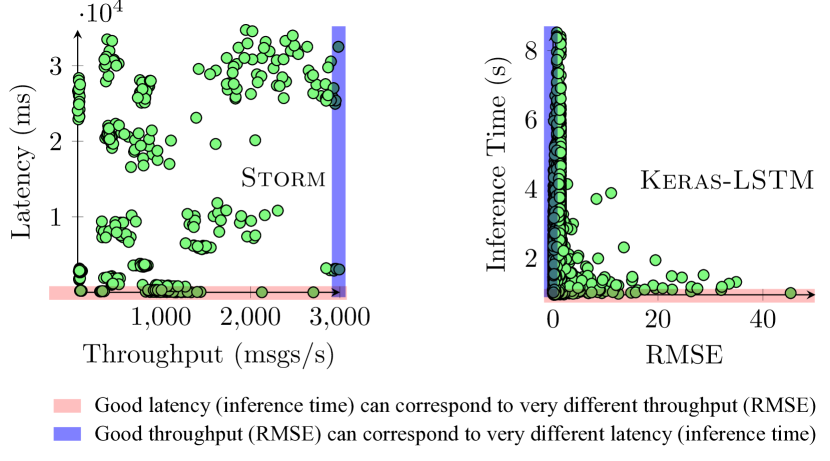
Figure 2. Measured configurations for Storm and Keras-LSTM. The points that Property 3 refers to are highlighted: very good or bad results on one performance objective can both correspond to similarly good value on the other.

3.2. Plain Multi-Objectivization Model (PMO)

A straightforward idea to perform multi-objectivization is to add an auxiliary objective to optimize, along with the target objective. This is what has been commonly used in other SBSE scenarios (e.g., (Derakhshanfar et al., 2020)). That PMO model can be formulated as:

(2) $$\begin{split}\text{minimize}\begin{cases}f_{t}(\boldsymbol{x})\\ f_{a}(\boldsymbol{x})\\ \end{cases}\end{split}$$

where $f_{t}(\boldsymbol{x})$ denotes the target performance objective (i.e., the concerned one) and $f_{a}(\boldsymbol{x})$ denotes the auxiliary performance objective.

Putting in the context of software configuration tuning, the PMO model may cover Property 1, because the natural Pareto relation ensures that the target performance objective is no longer a sole indicator to guide the search. However, it does not fit Property 2 as PMO additionally optimizes the auxiliary performance objective. As such, configurations that perform well on the auxiliary performance objective but poorly on the target performance objective are still regarded as optimal in PMO, despite being meaningless to the original problem. This can result in a significant waste of resources. In addition, PMO does not consider Property 3 as it often assumes conflicting correlation between the two objectives (Mkaouer et al., 2014; Derakhshanfar et al., 2020), which is hard to assure in software configuration tuning.

3.3. Our Meta Multi-Objectivization Model

Unlike PMO, our meta multi-objectivization (MMO) model creates two meta-objectives based on the performance attributes. The aim is to drive the search towards the optimum of the target performance objective, and at the same time, not being trapped in local optima. Specifically, we want to achieve two goals:

• Goal 1: optimizing the target performance objective still plays a primary role, thus no resource waste on, for example, optimizing the auxiliary one (this fits in Property 2);

• Goal 2: but those with different values of the auxiliary performance objective are more likely to be incomparable (i.e., Pareto nondominated), thus the search would not be trapped in local optima (this relates to Properties 1 and 3).

Formally, the proposed model with two meta-objectives $g_{1}(\boldsymbol{x})$ and $g_{2}(\boldsymbol{x})$ is constructed as:

(3) $$\begin{split}\text{minimize}\begin{cases}g_{1}(\boldsymbol{x})=f_{t}(\boldsymbol{x})+\varphi(f_{a}(\boldsymbol{x}))\\ g_{2}(\boldsymbol{x})=f_{t}(\boldsymbol{x})-\varphi(f_{a}(\boldsymbol{x}))\\ \end{cases}\end{split}$$

whereby each of the two meta-objectives shares the same target performance objective $f_{t}(\boldsymbol{x})$, but differs (effectively being opposite) regarding the auxiliary performance objective $f_{a}(\boldsymbol{x})$. $\varphi()$ is a composite function that balances the $f_{t}(\boldsymbol{x})$ and $f_{a}(\boldsymbol{x})$. In theory, the MMO model is generic and hence $\varphi()$ can take different forms to implement specific instances of the model. Here we consider its simplest instance $\varphi(f_{a}(\boldsymbol{x}))=wf_{a}(\boldsymbol{x})$ (we will investigate other instances in Section 4). That is,

(4) $$\begin{split}\text{minimize}\begin{cases}g_{1}(\boldsymbol{x})=f_{t}(\boldsymbol{x})+wf_{a}(\boldsymbol{x})\\ g_{2}(\boldsymbol{x})=f_{t}(\boldsymbol{x})-wf_{a}(\boldsymbol{x})\\ \end{cases}\end{split}$$

where $w$ is a weight parameter that allows fine-tuning of the balance; different systems may need different settings. Note that in the MMO model, both the target and the auxiliary performance objectives need to be normalized for commensurability.

To understand the proposed MMO model, Figure 3 gives an example of Storm on how it distinguishes between different configurations, in comparison with the PMO model, when using latency as the target performance objective $f_{t}$ and throughput as the auxiliary performance objective $f_{a}$. Suppose that there is a set of four configurations $\boldsymbol{A}$, $\boldsymbol{B}$, $\boldsymbol{C}$ and $\boldsymbol{D}$. Let us say if we want to choose two of them based on their fitness (e.g., in order to put some promising configurations into the next-generation population). For the PMO model (Figure 3a) that minimizes latency and maximizes throughput, the configuration $\boldsymbol{D}$, which performs extremely poor on latency, will certainly be chosen by any multi-objective optimizer, since it is Pareto optimal and also less crowded than the other Pareto optimal configuration $\boldsymbol{A}$ and $\boldsymbol{B}$. In contrast, for our MMO model (Figure 3b) which minimizes the two meta objectives, the two configurations that will be chosen are $\boldsymbol{A}$ and $\boldsymbol{C}$ since they are the only two Pareto optimal ones.

It is worth noting that for the single-objective optimization model (which only considers latency), the two chosen configurations will be $\boldsymbol{A}$ and $\boldsymbol{B}$. However, since $\boldsymbol{C}$ and $\boldsymbol{A}$ behave much more differently than $\boldsymbol{B}$ and $\boldsymbol{A}$ on the throughput, it is often more likely that they are located in distant regions in the configuration landscape; thus preserving $\boldsymbol{C}$ rather than $\boldsymbol{B}$ (when $\boldsymbol{A}$ is preserved) is generally more likely to help the search to escape from the local optimum.

(a) The original target-auxiliary space	(b) Our meta bi-objective space

Figure 3. An illustration of comparison between (a) the PMO model and (b) our MMO model (with the instance of Equation 4) on Storm, where the target performance objective is latency (to minimize) and the auxiliary performance objective is throughput (to maximize). Both of them are normalized and the weight is $0.5$ in MMO. Let us say $\boldsymbol{A}$, $\boldsymbol{B}$, $\boldsymbol{C}$ and $\boldsymbol{D}$ be a set of four configurations to be selected by the two models. The solid circle means the configuration being Pareto optimal to the set. Since the PMO model directly minimizes latency and maximizes throughput (Figure 3a), configurations $\boldsymbol{A}$, $\boldsymbol{B}$, and $\boldsymbol{D}$ are Pareto optimal. However, $\boldsymbol{D}$ performs very poorly on latency; preserving it during the search is a waste of resources. In contrast, in our MMO model (Figure 3b), configurations $\boldsymbol{A}$ and $\boldsymbol{C}$ are Pareto optimal. Now comparing configurations $\boldsymbol{C}$ with $\boldsymbol{B}$, since $\boldsymbol{C}$ and $\boldsymbol{A}$ behave much more differently than $\boldsymbol{B}$ and $\boldsymbol{A}$ on the throughput, it is often more likely that they are located on distant regions in the configuration landscape; thus preserving $\boldsymbol{C}$ rather than $\boldsymbol{B}$ (in case $\boldsymbol{A}$ is preserved) is generally more likely to avoid the search being trapped in the local optimum.

By further help to grasp the characteristics of the MMO model, we provide five remarks below. Remarks 1–3 are related to why the target performance objective remains primary in the model (Goal 1). Remarks 4 and 5 show how it helps to escape local optima via creating “incomparability” between the configurations with dissimilar values on the auxiliary performance objective (Goal 2).

Remark 1: The global optimum of the original single-objective problem (i.e., the configuration with the best target performance objective) is Pareto optimal in MMO (e.g., the configuration $\boldsymbol{A}$ in the example of Figure 3). This can be immediately obtained by contradiction from Equation (3).

Remark 2: A similar but more general observation is that a configuration will never be dominated by another that has a worse target performance objective. This can also be derived from Equation (3) — If configuration $\boldsymbol{x_{1}}$ has a better target performance objective than $\boldsymbol{x_{2}}$ (i.e., $f_{t}(\boldsymbol{x_{1}})<f_{t}(\boldsymbol{x_{2}})$), then whatever their auxiliary performance objective values are, $\boldsymbol{x_{2}}$ will not be better than $\boldsymbol{x_{1}}$ on both $g_{1}$ and $g_{2}$; in the best case for $\boldsymbol{x_{2}}$, they are nondominated to each other (e.g., the configuration $\boldsymbol{B}$ versus $\boldsymbol{C}$ in Figure 3).

Remark 3: The above two remarks apply to the target performance objective, but not to the auxiliary performance objective. This is a key difference from the PMO model, where both objectives are subject to these remarks; thus the configuration $\boldsymbol{D}$ in the example of Figure 3, which is meaningless to the original problem, is treated as being optimal in PMO but not in MMO.

Remark 4: MMO does not bias to a higher or lower value on the auxiliary performance objective, in contrast to PMO. This makes sense since, as explained in Property 3, we do not know for certain that what value of the auxiliary performance objective corresponds to the best target performance objective.

Remark 5: Configurations with dissimilar auxiliary performance objective values tend to be incomparable (i.e., nondominated to each other) even if one is fairly inferior to the other on the target performance objective. For example, the configuration $\boldsymbol{C}$ in Figure 3, which has worse latency than $\boldsymbol{A}$, is not dominated by $\boldsymbol{A}$ as their throughput are rather different. In contrast, the configuration $\boldsymbol{B}$, which even has better latency than $\boldsymbol{C}$, is dominated by $\boldsymbol{A}$, as they are similar on throughput. This enables the model to keep exploring diverse promising configurations during the search, thereby a higher chance to find the global optimum.

4. Experimental Setup

In this section, we articulate the experimental methodology for evaluating our MMO model and its instances.

4.1. Research Questions

Our experiment investigates the following research questions (RQs):

• RQ1: How effective is the MMO model?

• RQ2: How resource-efficient is the MMO model?

• RQ3: What is the sensitivity of the MMO model to its weight?

We ask RQ1 to verify whether our MMO model can better help to overcome the issue of local optima, i.e., by providing better results than the single-objective counterpart and PMO under the same search budget. We investigate RQ2 to examine whether the resources (the number of measurements) are consumed to reach a certain level of performance in a reasonably efficient manner. We use RQ3 to study whether the weight in MMO is critical.

Table 1. Configurable software systems studied.

Software	Domain	Performance Objective	$\lvert\mathbfcal{O}\rvert$	Search Space
Trimesh	Mesh	O1: # Iteration; O2: Latency	13	239,260
x264	Video	O1: PSNR; O2: Energy Usage	17	53,662
Storm/WC	SP	O1: Throughput; O2: Latency	6	2,880
Storm/RS	SP	O1: Throughput; O2: Latency	6	3,839
Storm/SOL	SP	O1: Throughput; O2: Latency	13	2,048
Keras-DNN/DSR	DL	O1: AUC; O2: Inference Time	13	3.32$\times 10^{13}$
Keras-DNN/Coffee	DL	O1: AUC; O2: Inference Time	13	2.66$\times 10^{13}$
Keras-LSTM	DL	O1: RMSE; O2: Inference Time	13	7,040

• $\lvert\mathbfcal{O}\rvert$ denotes number of options. We run all systems under their standard benchmarks. More details can be found at: https://github.com/taochen/mmo-fse-2021.

4.2. Subject Software Systems

As shown in Table 1, we experiment on a set of commonly used real-world software systems and environments (Nair et al., 2020; Jamshidi and Casale, 2016; Mendes et al., 2020; Jamshidi et al., 2018), whose single measurement is expensive. They come from diverse domains, e.g., stream processing (SP) and deep learning (DL), while having different performance attributes, scale, and search space.

Each software system comes with two performance objectives, which are chosen arbitrarily from prior work (Nair et al., 2020; Jamshidi and Casale, 2016; Mendes et al., 2020; Jamshidi et al., 2018). In all experiments, we use each of their two performance attributes as the target performance objective in turn while the other serves as the auxiliary performance objective.

We use the same configuration options and their ranges as studied in the prior work (Nair et al., 2020; Jamshidi and Casale, 2016; Mendes et al., 2020; Jamshidi et al., 2018), since those have been shown to be the key ones for the software systems under the related environment. As a result, although some subject software appears to be the same, their actual search spaces are different, such as Storm/WC and Storm/RS.

4.3. Tuning Settings

4.3.1. Models, MMO Instances and Optimizers

For the single-objec-tive optimization model, we examine four state-of-the-art optimizers that are widely used in software configuration tuning, all of which deal with local optima in different ways:

• Random Search (RS) with a high neighbourhood radius to escape from the local optima (Bergstra and Bengio, 2012; Ye and Kalyanaraman, 2003; Oh et al., 2017).

• Stochastic Hill Climbing with restart (SHC-r) (Xi et al., 2004; Li et al., 2014), aiming to avoid local optima by using different starting points.

• Single-Objective Genetic Algorithm (SOGA) (Behzad et al., 2013; Shahbazian et al., 2020) that seeks to escape local optima by using variation operators.

• Simulated Annealing (SA) (Ding et al., 2015; Guo et al., 2010) that tackles local optima by stochastically accepting inferior configurations.

Recall from Equation (2), our MMO model can be instantiated in different forms. In the experiments, we consider three alternatives:

• MMO-Linear: $\varphi(f_{a}(\boldsymbol{x}))=wf_{a}(\boldsymbol{x})$.

• MMO-Sqrt: $\varphi(f_{a}(\boldsymbol{x}))=w\sqrt{f_{a}(\boldsymbol{x})}$.

• MMO-Square: $\varphi(f_{a}(\boldsymbol{x}))=wf_{a}^{2}(\boldsymbol{x})$.

We examine all the above instances of the MMO model, together with the PMO. While our model does not tie to any specific multi-objective optimizer, we use NSGA-II for both MMO and PMO in this work, because (1) it has been predominately used for software configuration tuning in prior work when multiple performance attributes are of interest (Chen et al., 2018d; Singh et al., 2016; Chen et al., 2019; Kumar et al., 2018; Sobhy et al., 2020); (2) it shares many similarities with the SOGA that we compare in this work. Note that MMO may not be able to work with some multi-objective optimizers specifically designed for SBSE problems where the objectives are not treated equally, such as (Panichella et al., 2015; Hierons et al., 2016; Hierons et al., 2020).

All those optimizers can, but do not have to, rely on a surrogate. Since we focus on the optimization model, the ability to omit the surrogate model is desirable, as it has been shown that such a surrogate can be highly inaccurate (Zhu et al., 2017) and hence creates noises in our experiments. In this work, all optimization models and optimizers are implemented in Java, using jMetal (Durillo and Nebro, 2011) and Opt4J (Lukasiewycz et al., 2011).

4.3.2. Weight Values

In our experiments, we evaluate a set of weight values, i.e., $w\in\{0.01,0.1,0.3,0.5,0.7,0.9,10\}$, for all MMO instances. Those are merely pragmatic settings without any sophisticated reasoning. In this way, we aim to examine whether the MMO model can be effective by choosing from some randomly given weight values. To make the performance objectives commensurable in MMO, we use max-min scaling (Dodge and Commenges, 2006). However, since the bounds are often unknown, we update them dynamically as the tuning proceeds; this is a widely used approach in SBSE (Shahbazian et al., 2020).

4.3.3. Search Budget

Since the measurement is expensive, we repeat all experiments 30 runs with a search budget of 2 hours each, as suggested in prior work (Jamshidi and Casale, 2016). However, directly using the time as a termination criterion would cause the search to suffer non-trivial interference given the number of experiments we need to run in parallel. To avoid this, for each software system, we incrementally (100 each step) measured distinct configurations on a dedicated machine using random sampling until the time budget is exhausted. In this way, we collect the number of measurements (the median of 5 repeats), as shown in Table 2, that serve as the termination criterion for the configuration tuning thereafter.

Since the search budget reflects the number of measurements permitted in 2 hours, in each run, we cached the measurement of every distinct configuration, which can be reused directly when the same configuration appears again during the search. In other words, only the distinct configurations would consume the budget.

4.3.4. Other Parameters

For SOGA and NSGA-II, we apply the binary tournament for mating selection, together with the boundary mutation and uniformed crossover, as used in prior work (Chen et al., 2018d; Shahbazian et al., 2020; Chen et al., 2019). The mutation and crossover rates are set to 0.1 and 0.9, respectively, as commonly set in software configuration tuning (Chen et al., 2018d).

However, what we could not decide easily is the population size for SOGA and NSGA-II. Therefore, for each software system, we examine different population sizes, i.e., $\{10,20,...,100\}$ in preliminary runs. We used the largest size that enables the population change to be less than 10% in the last 10% of the generations over both optimizers, performance objectives, and weights. The results are shown in Table 2. In this way, we seek to reach a good balance between convergence (smaller population change) and diversity (larger population size) under a search budget.

Table 2. Population size and measurement search budget.

Software	Pop. Size	Budget	Software	Pop. Size	Budget
Trimesh	20	1000	x264	50	2,500
Storm/WC	50	600	Storm/RS	50	900
Storm/SOL	50	700	Keras-DNN/DSR	60	800
Keras-DNN/Coffee	50	900	Keras-LSTM	20	400

4.4. Comparison and Statistical Test

4.4.1. Metric

Since only the target objective is of interest, we do not need to consider the quality of the auxiliary objective (Li et al., 2020a). We use the average normalized percentage gain (Hake, 1998) of the target objective on the MMO (or PMO) model against on the single-objective counterpart, which is defined as:

(5) $$\text{Normalized \% Gain}={{1\over n}\times\sum^{n}_{i=1}{{y_{i}-x_{i}}\over{y_{i}-y_{o}}}}\times 100$$

whereby $x_{i}$ and $y_{i}$ are the objective value of the single performance concern at the $i$th run for a multi-objectivization model and the best (average) single-objective counterpart, respectively. $y_{o}$ is an utopian performance that none of the optimizers can achieve. In this work, we set $y_{o}=v_{o}-q$ wherein $v_{o}$ is the optimal performance value found from all optimizers; and $q$ is the distance of the closest sample $s$ to $v_{o}$ over all cases, such that $s\neq v_{o}$. Clearly, when the normalized % gain is zero or negative, it implies that the multi-objectivization model is similar or even worse off, respectively. Note that the objective values are sorted for a total of $n$ runs where $n=30$. According to Hake (Hake, 1998), the normalized % gain is a more suitable metric than its non-normalized version (without $y_{o}$) because:

• It has been used as a standard metric in many domains (Hake, 1998).

• It can more accurately capture the spread (Marx and Cummings, 2007).

• More importantly, it rewards (or penalizes) improvement (or degradation) more when the $y_{i}$ is closer to the (approximately) optimal value. For example, improving the latency from 100s to 50s shares the same non-normalized % gain as from 50s to 25s (i.e., 50%). However, given the severe issue of local optima in software configuration tuning, the latter case can be much more difficult to achieve than the former and hence deserves a greater reward. Suppose that the utopian performance is 20s in the above example, the normalized % gain for the two cases would be 62.5% and 83.3%, respectively.

4.4.2. Statistical Methods

We use the following statistical methods:

• Wilcoxon signed-rank test (Wilcoxon, 1945): We apply this with $a=0.05$ to investigate the statistical significance of the performance objective comparisons over all 30 runs, as it is a non-parametric statistical test and has been recommended in software engineering research for its strong statistical power on pair-wise comparisons (Arcuri and Briand, 2011). If the $p<0.05$, we say the magnitude of differences in the comparisons are significant.

• $\mathbf{\hat{A}_{12}}$ effect size (Vargha and Delaney, 2000): We use $\hat{A}_{12}$ to verify the effect size over 30 runs. When comparing a multi-objectivization model and its single-objective counterpart in this work, $\hat{A}_{12}>0.5$ denotes that the multi-objectivization is better for more than 50% of the times. In particular, $0.56\leq\hat{A}_{12}<0.64$ indicates a small effect size while $0.64\leq\hat{A}_{12}<0.71$ and $\hat{A}_{12}\geq 0.71$ mean a medium and a large effect size, respectively.

5. Evaluation Results

In this section, we present the results of our experimental evaluations and address the research questions posed in Section 4.1. The experiments were run in parallel on several machines each with six cores CPU at 2.9GHz and 8GB RAM for two months ($24\times 7$). All settings discussed in Section 4 are used unless otherwise stated.

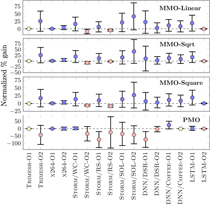
Figure 4. Average and standard deviations on % gain of MMO and PMO over the best single-objective counterpart for 30 runs. The blue, pink, and yellow denote positive, negative, and zero average gain, respectively.

5.1. RQ1: Effectiveness

5.1.1. Method

To answer RQ1, we examine all the eight software systems/environments with two performance objectives each, giving us 16 cases of study. In each case, we compare the best single-objective counterpart with all instances of MMO and PMO. To set the weight for each MMO instance in a case, we firstly conduct preliminary runs under 10% of the search budget and population size (one run each value). The weight with the best target performance objective is then used in the full-scale experiments (if more than one weight is the best, we chose one randomly). For all pair-wise comparisons, both Wilcoxon sign-rank test and $\hat{A}_{12}$ are used.

Table 3. $\hat{A}_{12}$ and $p$ values on comparing multi-objectivization (MMO and PMO model) against the best single-objective counterpart over 30 runs.

Software System	MMO-Linear	MMO-Sqrt	MMO-Square	PMO
Trimesh-O1	.50 ($<$.001)	.50 ($<$.001)	.50 ($<$.001)	.50 ($<$.001)
Trimesh-O2	.88 ($<$.001)	.93 ($<$.001)	.88 ($<$.001)	.25 ($=$.002)
x264-O1	.80 ($<$.001)	.73 ($<$.001)	.97 ($<$.001)	.85 ($<$.001)
x264-O2	.78 ($<$.001)	.82 ($<$.001)	.77 ($<$.001)	.40 ($=$.918)
Storm/WC-O1	.67 ($<$.001)	.68 ($<$.001)	.65 ($<$.001)	.53 ($<$.001)
Storm/WC-O2	.03 ($<$.001)	.02 ($<$.001)	.00 ($<$.001)	.33 ($=$.636)
Storm/RS-O1	.57 ($<$.001)	.62 ($<$.001)	.60 ($<$.001)	.10 ($<$.001)
Storm/RS-O2	.00 ($<$.001)	.17 ($<$.001)	.02 ($<$.001)	.47 ($<$.001)
Storm/SOL-O1	.67 ($<$.001)	.62 ($<$.001)	.62 ($<$.001)	.40 ($=$.334)
Storm/SOL-O2	.72 ($<$.001)	.72 ($<$.001)	.65 ($<$.001)	.28 ($=$.100)
Keras-DNN/DSR-O1	.67 ($=$.001)	.62 ($=$.031)	.53 ($=$.008)	.05 ($<$.001)
Keras-DNN/DSR-O2	.52 ($<$.001)	.52 ($<$.001)	.52 ($<$.001)	.48 ($<$.001)
Keras-DNN/Coffee-O1	.67 ($<$.001)	.68 ($<$.001)	.67 ($<$.001)	.73 ($<$.001)
Keras-DNN/Coffee-O2	.58 ($<$.001)	.58 ($<$.001)	.58 ($<$.001)	.50 ($<$.001)
Keras-LSTM-O1	.68 ($<$.001)	.70 ($<$.001)	.72 ($<$.001)	.53 ($<$.001)
Keras-LSTM-O2	.48 ($=$.002)	.48 ($=$.002)	.58 ($<$.001)	.42 ($=$.056)

• The $p$ values are shown in the bracket. $\hat{A}_{12}>0.5$ means the MMO (or PMO) is better (in blue); $\hat{A}_{12}<0.5$ denotes the best single-objective counterpart is better (in pink); $\hat{A}_{12}=0.5$ means a tie. The comparisons, for which there is a $p<$0.05 and $\hat{A}_{12}\leq 0.44$ or $\hat{A}_{12}\geq 0.56$, are highlighted in bold.

5.1.2. Results

From Figure 4, we see that, on average, the MMO model achieves reasonably positive gains for at least 12 cases across the instances. This is a sign that the MMO model suffers less on the local optima issue than its best single-objective counterpart. Moreover, it achieves improvements for more than an average of 30% in some cases, e.g., Storm/SOL-O2, as in those cases the distance between local optima can be large. Yet, we observe no obvious difference among the MMO instances. PMO, albeit leads to acceptable results for some cases, often performs worse than the best single-objective counterpart as the gains are generally similar or negative (11 out of 16 cases). This can be attributed to the fact that it wastes a significant amount of resources on optimizing the auxiliary performance objective. Interestingly, for Trimesh-O1, all the models have the same results as the best single-objective counterpart. Although rare, this is a possible case where the landscape of the target performance objective is simpler (e.g., fewer local optima); hence all the models/optimizers can find the globally optimal configuration.

Table 3 shows the results of the statistical tests, in which we see that similar to the gains, the MMO model wins a larger majority in general, in which most of them are statistically significant ($p<0.05$) with non-trivial effect size ($\hat{A}_{12}\geq 0.56$). Again, the PMO performs the worst with no wins on 12 out of 16 cases.

To provide a detailed understanding, Figure 5 shows all the explored configurations for Trimesh with latency as the target performance objective. Clearly, we see that the result confirms our theory: the single-objective counterparts do explore some good ranges of configurations, but they remain mostly trapped in a large region of local optima. The PMO performs the worst with fewer points in the projected area because it over-empathizes on optimizing the auxiliary performance objective, which negatively affects the target performance objective. Our MMO model, in contrast, escapes from local optima by exploring an even larger area while keeping the tendency towards better target performance objective, which is precisely our Goals 1 and 2 from Section 3. Therefore, we say:

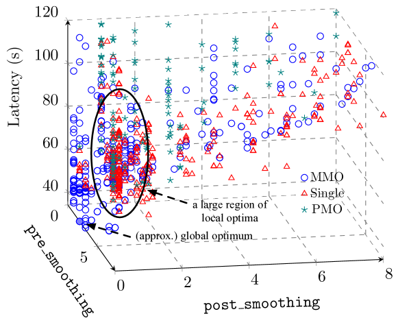
Figure 5. A projected landscape of Trimesh explored by MMO (since all instances perform similarly, here we use MMO-Linear as an example), PMO, and the best single-objective counterpart. Each point is a configuration measured in the run, regardless whether it is preserved or not.

5.2. RQ2: Resource Efficiency

5.2.1. Method

To investigate RQ2, for each case, we use a baseline, $b$, taken as the smallest number of measurements that the best single-objective counterpart consumes to achieve its best average result over 30 runs. We then record the smallest amount of budget consumed by the MMO and PMO to achieve the same (or better) target performance objective on average, denoted as $m$. The ratios, i.e., $r={m\over b}\times 100\%$, are reported, implying that if the MMO instances are resource-efficient, then we would expect $r\leq 100\%$. Since in our context the resource is the number of measurements, it reflects the tuning time and computation required by a model. Again, as for RQ1, only the best weight for each MMO instance identified from the preliminary runs is examined in a case.

5.2.2. Results

As can be seen from Figure 6, despite a small number of cases where the MMO model cannot reach the performance level as achieved by the best single-objective counterpart (the divided bars, denoted as $r\gg 100\%$), most commonly it uses less number of measurements than, or at least identical to, the baseline to find the same or better results, e.g., it can be as significantly low as 24%. In particular, the MMO instances have 10-13 cases of $r<100\%$; 1-3 cases of $r=100\%$; and 2-3 cases of $r\gg 100\%$. This indicates that the MMO model overcomes local optima better and more efficiently — a key attraction to software configuration tuning due to its expensive measurements. In contrast, the PMO exhibits the worst resource efficiency, as it has 3 cases of $r<100\%$, together with 1 and 2 cases of $r=100\%$ and $r>100\%$, respectively, while the remaining 10 cases of $r\gg 100\%$. This is a clear sign that PMO is generally resource-hungry as discussed in Section 3.

Notably, the resource saving of MMO is more significant on systems with larger search space, e.g., Keras-DNN and Trimesh. This is because that the larger the search space, the more the resources are required for the single-objective model to find good configurations. In contrast, our model MMO, which is designed to keep a set of diverse high-quality configurations during the tuning, needs less effort to find better ones. As a result, we conclude that:

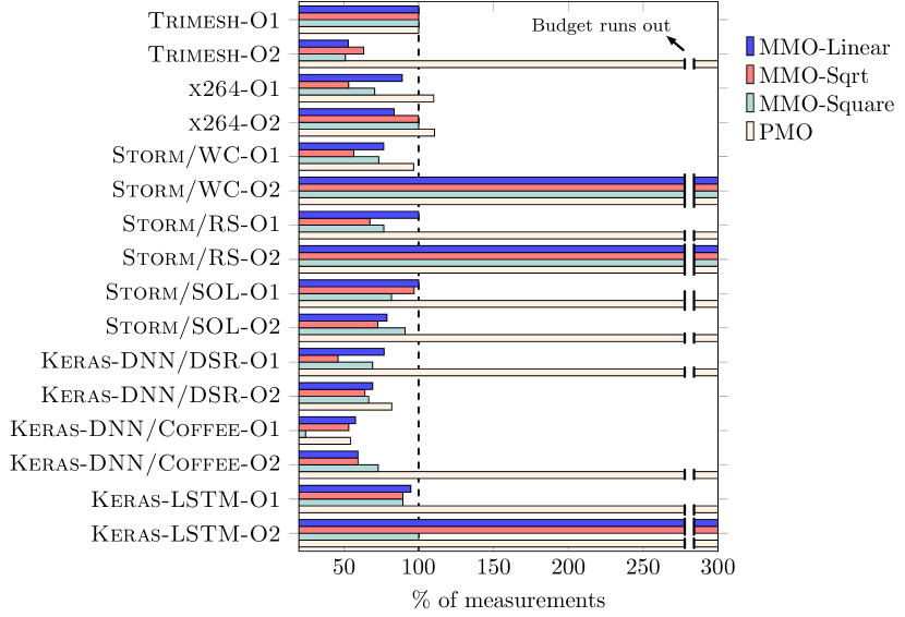
Figure 6. % of measurements ($r$) for the MMO and PMO models to converge to the best (average) performance objective by the best single-objective counterpart over 30 runs, using its budget consumption as the baseline (the dashed line). The divided bars denote no convergence when the total search budget runs out, i.e., $r\gg 100\%$.

5.3. RQ3: Sensitivity to Weight

5.3.1. Method

To address RQ3, we check how do the MMO instances perform compared with the best single-objective counterpart under different weight settings for the full-scale experiments. Hence, for each instance, there are seven settings and 16 systems/environments, leading to 112 cases. In each of these cases, we conduct a pair-wise comparison using the $\hat{A}_{12}$ and Wilcoxon sign-rank test.

5.3.2. Results

The results are shown in Table 4, in which we see that the MMO model, regardless to its instance, may indeed be sensitive to the weight as it could win or lose (with different $\hat{A}_{12}$ values and statistical results) depending on different settings. Although the best weight can be different for specific cases, we do observe a general pattern: according to the last row, setting the weight as an edge value like 0.01, 0.1, 0.9, or 10 tends to be the best among others in general. This is clearer for MMO-Linear and MMO-Sqrt, while MMO-Square prefers 0.01 more. We also note that the best weights identified from the preliminary runs are generally consistent with those best ones under the full-scale experiments.

In particular, we see that all the MMO instances can be more beneficial (more weight values, if not all, can lead to significantly better results) in some cases of the complex systems (e.g., x264 and Keras-DNN) than others with smaller search space and dimension of options (e.g., Storm). This could be due to the fact that for more challenging systems, the advantage of our model over the single-objective counterpart is clearer, thus it is easier to have a better result over different weight settings. In summary, we state that:

6. Discussion

6.1. Why Software Configuration Tuning?

A natural question to ask is why our MMO model is specific for software configuration tuning rather than as a general “search-based” solution for all SBSE problems. The answer is three-fold.

Firstly, we took three important properties of software configuration tuning into account when designing the MMO model: (1) the high degree of sparsity in software systems exacerbates the issue of the search being trapped in local optima (Property 1) (Nair et al., 2020; Jamshidi and Casale, 2016). (2) The measurement is expensive; thus efficiently escaping the local optima with less resources is desirable (Property 2). (3) The correlations between performance attributes are uncertain, i.e., extremely well or poor auxiliary performance objective may both lead to similarly good target performance objective (Property 3).

Table 4. Sensitivity analysis on different weights in the MMO model (full-scale experiments). The cells report the $\hat{A}_{12}$ values and whether $p<0.05$ on comparing a MMO instance and the best single-objective counterpart over 30 runs. The last row counts how many times a weight value is the best in a case based on Scott-Knott rank (primary) and the average result (secondary).

Software System

MMO-Linear

MMO-Sqrt

MMO-Square

0.01

0.1

0.3

0.5

0.7

0.9

10

0.01

0.1

0.3

0.5

0.7

0.9

10

0.01

0.1

0.3

0.5

0.7

0.9

10

Trimesh-O1

.50†

.50†

.50†

.50†

.50†

.50†

.50†

.50†

.50†

.50†

.50†

.50†

.50†

.50†

.50†

.50†

.50†

.50†

.50†

.50†

.50†

Trimesh-O2

.75†

.88†

.07†

.00†

.00†

.00†

.00†

.35

.93†

.20†

.00†

.05†

.08†

.05†

.88†

.00†

.02†

.02†

.00†

.05†

.02†

x264-O1

.83†

.90†

.82†

.80†

.87†

.88†

.80†

.95†

.93†

.90†

.88†

.85†

.82†

.73†

.88†

.87†

.80†

.83†

.97†

.88†

.72†

x264-O2

.58†

.60†

.38

.78†

.50

.45

.48

.47

.42

.27†

.45

.40

.58†

.82†

.77†

.47

.50

.53†

.40

.48

.43

Storm/WC-O1

.39

.62†

.45†

.43†

.67†

.63†

.33

.58†

.52†

.52†

.43†

.53†

.68†

.38

.58†

.58†

.60†

.65†

.53†

.52†

.30

Storm/WC-O2

.03†

.00†

.00†

.00†

.00†

.00†

.02†

.02†

.00†

.02†

.00†

.00†

.00†

.00†

.00†

.03†

.02†

.00†

.02†

.00†

.02†

Storm/RS-O1

.55†

.52†

.42

.48†

.57†

.57†

.10†

.55†

.55†

.53†

.52†

.53†

.62†

.18†

.57†

.60†

.57†

.50†

.53†

.52†

.22†

Storm/RS-O2

.00†

.00†

.00†

.00†

.02†

.00†

.00†

.17†

.00†

.00†

.00†

.00†

.00†

.00†

.02†

.00†

.00†

.00†

.00†

.00†

.00†

Storm/SOL-O1

.43†

.45†

.47†

.57†

.67†

.58†

.18†

.45†

.47†

.40

.52†

.62†

.55†

.18†

.38

.48†

.50†

.43†

.45†

.62†

.52†

Storm/SOL-O2

.72†

.53†

.43

.53†

.42

.30

.17†

.72†

.55†

.53†

.38

.38

.25†

.17†

.65†

.55†

.38

.45

.35

.28

.33

Keras-DNN/DSR-O1

.22†

.33

.45

.57†

.47

.20†

.67†

.30

.25†

.28†

.33

.42

.47

.62†

.28

.32

.25†

.17†

.28†

.28†

.53†

Keras-DNN/DSR-O2

.52†

.52†

.52†

.43†

.38

.37

.28

.52†

.52†

.47†

.47†

.40

.37

.45†

.52†

.52†

.43†

.45†

.40

.35

.38

Keras-DNN/Coffee-O1

.43

.53†

.58†

.50†

.45

.67†

.55†

.47†

.50†

.68†

.55†

.57†

.60†

.58†

.38

.43

.52†

.55†

.58†

.67†

.52†

Keras-DNN/Coffee-O2

.58†

.58†

.58†

.58†

.57†

.57†

.57†

.58†

.57†

.58†

.57†

.57†

.53†

.50†

.58†

.58†

.53†

.57†

.55†

.58†

.57†

Keras-LSTM-O1

.68†

.58†

.47†

.30

.47†

.47†

.38

.32

.70†

.35

.48†

.32

.42

.58†

.47†

.35

.72†

.47†

.32

.45†

.28

Keras-LSTM-O2

.37

.38

.48†

.45†

.32

.47†

.38

.42

.30

.33

.42

.28

.48†

.33

.28

.58†

.37

.32

.35

.45†

.35

$\#$ Best (over 16 cases)

4

2

1

2

2

2

3

3

3

2

0

1

4

3

6

2

1

1

1

3

2

• ^† denotes a statistically significant comparison with $p<0.05$. Other formats are the same as Table 3.

Secondly, the configurable software systems provide a well-fitting avenue for multi-objectivization, as it is common that they inherently come with at least two performance attributes, e.g., latency and throughput, that can be directly used in the multi-objectivization. Some other SBSE problems, in contrast, may not have a readily available attribute(s) that can serve as the auxiliary objective. For example, in the code refactoring problem, the robustness of the code (as an auxiliary objective) is not a straightforward and widely known metric that can be easily quantified (Mkaouer et al., 2014).

Finally, how the configurations can affect the performance attributes is often a black-box. In contrast, in many other SBSE problems, the objective function can be specifically designed based on some shared domain properties between scenarios. For example, in crash reproduction problem (Derakhshanfar et al., 2020), it is possible to engineer a new auxiliary objective to check how widely a test case covers the code based on some common code structures for a software system (e.g., function access levels), such that it is strongly conflicting with the target objective (i.e., distance to the particular line(s)-of-code that reproduces the crash). However, it is difficult, if not impossible, for the configuration options in software configuration tuning to achieve the same. Our MMO model explicitly considers such a black-box nature of software configuration tuning, as we make no assumption about the performance attributes and their correlations.

Figure 7. The maximum running time for a full-scale run when using previously measured data to identify the best weight (over all seven weight values and 30 runs). ✓ denotes the best weight concluded using data is identical to that obtained from profiling the system; ✕ means otherwise.

6.2. How to Use MMO in Practice?

Here, we elaborate on the guidelines for using MMO in practice.

6.2.1. Choosing the MMO instance

Sections 5.1 and 5.2 reveal that the MMO instances perform similarly for software configuration tuning — all better than the best single-objective counterpart and PMO in general. It is, therefore, safe to choose any of them. In general, we suggest to use MMO-Linear by default as it is the simplest form among the others.

6.2.2. Setting the weight

We recommend two alternative methods to identify the best weights during preliminary runs: physically profiled method and data-driven method.

To set a good weight, one can profile the actual system with a reduced budget (e.g., 10%), as what we have done in this work. In fact, the findings from Section 5.3 has provided useful insights to simplify the process: albeit the difficulty of setting weight varies depending on the case, we observed that the edge weight value, e.g., 0.01, 0.1, 0.9 or 10, is generally a reliable setting. Further, there are also cases where nearly all weights we examined are highly effective, such as x264-O1 and Keras-DNN/Coffee-O2. Therefore, we suggest trying at least the above values in the preliminary runs.

When previously measured data is available, the data-driven method for identifying the weight becomes possible. We have found that, for all the MMO instances and cases under the full-scale experiments, the best weight value concluded based on the data is the same as that identified by measuring the system, but the former can terminate several orders of magnitude faster. As shown in Figure 7, when examining the weight using all data collected from the previous experiments, we see that the resulted best weights are generally consistent with those identified by physically profiling the systems (as in Section 5.3). For the few cases where there is an inconsistency, all the weights in fact perform rather similar (e.g., x264-O1), therefore it is safe even if the actual best one has not been chosen. More importantly, the maximum running time is negligible when using data — it is merely 3 seconds or less.

6.3. Threats to Validity

Threats to internal validity can be related to the search budget. To tackle this, we have used two-hour budgets as suggested in prior work (Jamshidi and Casale, 2016). The parameter settings follow what has been used from the literature or tuned through preliminary runs. To mitigate bias, we repeated 30 experiment runs under each case.

The metrics and evaluation used may pose threats to construct validity. Since there is only a single performance concern, we conduct the comparison based on the gains on the target performance objectives over the best single-objective optimizer, together with the resources (number of measurements) required to converge to the same result. Both of these are common metrics in software configuration tuning (Nair et al., 2020). To verify statistical significance and effect size, we use Wilcoxon sign-rank test and $\hat{A}_{12}$ to examine the results.

Threats to external validity can be raised from the subjects studied. We mitigated this by using eight systems/environments that are of different scales and performance attributes. We also compared the MMO model with four state-of-the-art single-objective counterparts for software configuration tuning. Nonetheless, we agree that using more systems and optimizers may prove fruitful.

7. Related Work

Broadly, optimizers for software configuration tuning can be classified into two categories: measurement-based and model-based.

Measurement-based Optimizers: In measurement-based methods, the optimizer is directly used to measure the configuration on the software systems. Despite the expensiveness, the measurements can accurately reflect the good or bad of a configuration. The optimizer can be based on random search (Bergstra and Bengio, 2012; Ye and Kalyanaraman, 2003; Oh et al., 2017), hill climbing (Xi et al., 2004; Li et al., 2014), single-objective genetic algorithm (Behzad et al., 2013; Shahbazian et al., 2020) and simulated annealing (Ding et al., 2015; Guo et al., 2010), to name a few. Under such a single-objective model, various tricks have been applied. For example, some extend random search to consider a wider neighboring radius of the configuration structure, hence it is more likely to jump out from the local optima (Oh et al., 2017). Others rely on restarting from a different point, such as in restarted hill climbing, hence increasing the chance to find the “right” path from local optima to the global optimum (Zhu et al., 2017; Xi et al., 2004).

Our MMO model differs from all the above as it lies in a higher level of abstraction — the optimization model — as opposed to the level of optimization method.

Model-based Optimizers: Instead of solely using the measurements of software systems, the model-based methods apply a surrogate model (analytical (Kumar et al., 2020; Chen et al., 2018c; Chen et al., 2019) or machine learning based (Nair et al., 2020; Jamshidi and Casale, 2016)) to evaluate configurations, which guides the search in an optimizer. The intention is to speed up the exploration of configurations as the model evaluation is rather cheap. Yet, it has been shown that the model accuracy and the availability of initial data can become an issue (Zhu et al., 2017). Among others, Jamshidi and Casale (Jamshidi and Casale, 2016) use Bayesian optimization to tune software configuration, wherein the search is guided by the Gaussian process regression trained from the data collected. Nair et al. (Nair et al., 2020) follow a similar idea but a regression tree model is used instead.

Since MMO lies in the level of optimization model, it is complementary to the model-based methods in which the MMO would take the surrogate values as inputs instead of the real measurements.

General Parameter Tuning: Optimizers proposed for the parameter tuning of general algorithms can also be relevant (Blot et al., 2019; Huang et al., 2020; Bezerra et al., 2020; Pushak and Hoos, 2018), including IRace (López-Ibánez et al., 2016), ParamILS (Hutter et al., 2009), SMAC (Hutter et al., 2011), GGA$++$ (Ansótegui et al., 2015), as well as their multi-objective variants, such as MO-ParamILS (Blot et al., 2016) and SPRINT-Race (Zhang et al., 2015). To examine a few examples, ParamILS (Hutter et al., 2009) relies on iterative local search — a search procedure that may jump out of local optima using strategies similar to that of SA and SHC-r. Further, a key contribution is the capping strategy, which helps to reduce the need to measure an algorithm under some problem instances, hence saving computational resources. This is one of the goals that we seek to achieve too. Similar to Nair et al. (Nair et al., 2020), SMAC (Hutter et al., 2011) uses Bayesian optimization but relying on a Random Forest model, which additionally considers the performance of an algorithms over a set of instances.

However, their work differs from ours in two aspects. Firstly, general algorithm configuration requires to work on a set of problem instances, each coming with different features. The software configuration tuning, in contrast, is often concerned with tuning software system under a given benchmark (i.e., one instance) (Nair et al., 2020; Jamshidi and Casale, 2016; Zhu et al., 2017; Chen et al., 2018d). Therefore, most of their designs for saving resources (such as the capping in ParamILS) were proposed to reduce the number of instances measured. Of course, it is possible to generalize the problem to consider multiple benchmarks as the same time, yet this is outside the scope of this paper. Secondly, none of them works on the level of optimization model, and therefore our MMO is still complementary to their optimizers.

Multi-Objectivization in SBSE: Multi-objectivization, which is the notion behind our MMO model, has been applied in other SBSE problems (Yuan and Banzhaf, 2020; Derakhshanfar et al., 2020; Mkaouer et al., 2014; Soltani et al., 2018). For example, to reproduce a crash based on the crash report, one can purposely design a new auxiliary objective, which measures how widely a test case covers the code, to be optimized alongside with the target crash distance (Derakhshanfar et al., 2020). A multi-objective optimizer, e.g., NSGA-II, is directly used thereafter. A similar case can be found also for the code refactoring problem (Mkaouer et al., 2014). However, during the tuning process, such a model, i.e., PMO in this paper, could waste a significant amount of the resources in optimizing the auxiliary objective, which is of no interest. This is a particularly unwelcome issue for software configuration tuning where the measurement is expensive. As we have shown in Section 5, PMO performs even worse than the classic single-objective model in most of the cases.

8. Conclusion and Future Work

This paper tackles the local optimum issue in software configuration tuning from a different perspective — multi-objectivizing the single objective optimization scenario. We do this by proposing a meta multi-objective model (MMO), at the level of optimization model (external part), as opposed to existing work that focuses on developing an effective single-objective optimizer (internal part). We compare MMO with four state-of-the-art single-objective optimizers and the plain multi-objectivization model over various scenarios. The results reveal that the MMO model:

• can generally be more effective in overcoming local optima;

• and do so by consuming less resources in most cases;

• can be sensitive to the weight, but there exist some commonly best values.

The idea of MMO is essentially to rotate the original space of target and auxiliary objectives hence that solutions with good target objective value and various auxiliary objective values incomparable. In this geometrical transformation, the weight parameter determines how far in terms of the auxiliary objective solutions are incomparable, relative to the target objective. A comparison with methods of the similar idea (e.g., select solutions with good target objective and diverse auxiliary objective values) can be beneficial as it can help answer an underlying question — can maintain the diversity of the auxiliary objective help optimization of the target one. This is one of our subsequent studies. Another direction of future work is to add more auxiliary objective. In this regard, how to do the transformation in the 3D space is the key. On top of the above, an adaptive weight adjustment approach for the MMO model, as suggested by the findings from RQ3, is certainly more desirable, which is worth investigating in depth.

- (1)
- Ahmad et al. (2018) Muhammad Aurangzeb Ahmad, Carly Eckert, and Ankur Teredesai. 2018. Interpretable Machine Learning in Healthcare. In Proceedings of the 2018 ACM International Conference on Bioinformatics, Computational Biology, and Health Informatics, BCB 2018, Washington, DC, USA, August 29 - September 01, 2018, Amarda Shehu, Cathy H. Wu, Christina Boucher, Jing Li, Hongfang Liu, and Mihai Pop (Eds.). ACM, 559–560. https://doi.org/10.1145/3233547.3233667
- Ansótegui et al. (2015) Carlos Ansótegui, Yuri Malitsky, Horst Samulowitz, Meinolf Sellmann, and Kevin Tierney. 2015. Model-Based Genetic Algorithms for Algorithm Configuration. In Proceedings of the Twenty-Fourth International Joint Conference on Artificial Intelligence, IJCAI 2015, Buenos Aires, Argentina, July 25-31, 2015, Qiang Yang and Michael J. Wooldridge (Eds.). AAAI Press, 733–739. http://ijcai.org/Abstract/15/109
- Arcuri and Briand (2011) Andrea Arcuri and Lionel C. Briand. 2011. A practical guide for using statistical tests to assess randomized algorithms in software engineering. In ICSE’11: Proc. of the 33rd International Conference on Software Engineering. ACM, 1–10.
- Behzad et al. (2013) Babak Behzad, Huong Vu Thanh Luu, Joseph Huchette, Surendra Byna, Prabhat, Ruth A. Aydt, Quincey Koziol, and Marc Snir. 2013. Taming parallel I/O complexity with auto-tuning. In International Conference for High Performance Computing, Networking, Storage and Analysis, SC’13, Denver, CO, USA - November 17 - 21, 2013, William Gropp and Satoshi Matsuoka (Eds.). ACM, 68:1–68:12. https://doi.org/10.1145/2503210.2503278
- Bergstra and Bengio (2012) James Bergstra and Yoshua Bengio. 2012. Random Search for Hyper-Parameter Optimization. J. Mach. Learn. Res. 13 (2012), 281–305. http://dl.acm.org/citation.cfm?id=2188395
- Bezerra et al. (2020) Leonardo C. T. Bezerra, Manuel López-Ibáñez, and Thomas Stützle. 2020. Automatic Configuration of Multi-objective Optimizers and Multi-objective Configuration. In High-Performance Simulation-Based Optimization, Thomas Bartz-Beielstein, Bogdan Filipic, Peter Korosec, and El-Ghazali Talbi (Eds.). Studies in Computational Intelligence, Vol. 833. Springer, 69–92. https://doi.org/10.1007/978-3-030-18764-4_4
- Blot et al. (2016) Aymeric Blot, Holger H. Hoos, Laetitia Jourdan, Marie-Éléonore Kessaci-Marmion, and Heike Trautmann. 2016. MO-ParamILS: A Multi-objective Automatic Algorithm Configuration Framework. In Learning and Intelligent Optimization - 10th International Conference, LION 10, Ischia, Italy, May 29 - June 1, 2016, Revised Selected Papers (Lecture Notes in Computer Science), Paola Festa, Meinolf Sellmann, and Joaquin Vanschoren (Eds.), Vol. 10079. Springer, 32–47. https://doi.org/10.1007/978-3-319-50349-3_3
- Blot et al. (2019) Aymeric Blot, Marie-Eléonore Marmion, Laetitia Jourdan, and Holger H. Hoos. 2019. Automatic Configuration of Multi-Objective Local Search Algorithms for Permutation Problems. Evol. Comput. 27, 1 (2019), 147–171. https://doi.org/10.1162/evco_a_00240
- Bogetoft (2013) Peter Bogetoft. 2013. Performance benchmarking: Measuring and managing performance. Springer Science & Business Media.
- Brown et al. (2020) Tom B Brown, Benjamin Mann, Nick Ryder, Melanie Subbiah, Jared Kaplan, Prafulla Dhariwal, Arvind Neelakantan, Pranav Shyam, Girish Sastry, Amanda Askell, et al. 2020. Language models are few-shot learners. arXiv preprint arXiv:2005.14165 (2020).
- Cai and Wang (2006) Zixing Cai and Yong Wang. 2006. A multiobjective optimization-based evolutionary algorithm for constrained optimization. IEEE Transactions on evolutionary computation 10, 6 (2006), 658–675.
- Chen (2019) Tao Chen. 2019. All versus one: an empirical comparison on retrained and incremental machine learning for modeling performance of adaptable software. In Proceedings of the 14th International Symposium on Software Engineering for Adaptive and Self-Managing Systems, SEAMS@ICSE 2019, Montreal, QC, Canada, May 25-31, 2019, Marin Litoiu, Siobhán Clarke, and Kenji Tei (Eds.). ACM, 157–168. https://doi.org/10.1109/SEAMS.2019.00029
- Chen and Bahsoon (2017a) Tao Chen and Rami Bahsoon. 2017a. Self-Adaptive and Online QoS Modeling for Cloud-Based Software Services. IEEE Trans. Software Eng. 43, 5 (2017), 453–475. https://doi.org/10.1109/TSE.2016.2608826
- Chen and Bahsoon (2017b) Tao Chen and Rami Bahsoon. 2017b. Self-Adaptive Trade-off Decision Making for Autoscaling Cloud-Based Services. IEEE Trans. Serv. Comput. 10, 4 (2017), 618–632. https://doi.org/10.1109/TSC.2015.2499770
- Chen et al. (2018b) Tao Chen, Rami Bahsoon, Shuo Wang, and Xin Yao. 2018b. To Adapt or Not to Adapt?: Technical Debt and Learning Driven Self-Adaptation for Managing Runtime Performance. In Proceedings of the 2018 ACM/SPEC International Conference on Performance Engineering, ICPE 2018, Berlin, Germany, April 09-13, 2018, Katinka Wolter, William J. Knottenbelt, André van Hoorn, and Manoj Nambiar (Eds.). ACM, 48–55. https://doi.org/10.1145/3184407.3184413
- Chen et al. (2018a) Tao Chen, Rami Bahsoon, and Xin Yao. 2018a. A Survey and Taxonomy of Self-Aware and Self-Adaptive Cloud Autoscaling Systems. ACM Comput. Surv. 51, 3 (2018), 61:1–61:40. https://doi.org/10.1145/3190507
- Chen et al. (2020) Tao Chen, Rami Bahsoon, and Xin Yao. 2020. Synergizing Domain Expertise With Self-Awareness in Software Systems: A Patternized Architecture Guideline. Proc. IEEE 108, 7 (2020), 1094–1126. https://doi.org/10.1109/JPROC.2020.2985293
- Chen et al. (2018d) Tao Chen, Ke Li, Rami Bahsoon, and Xin Yao. 2018d. FEMOSAA: Feature Guided and Knee Driven Multi-Objective Optimization for Self-Adaptive Software. ACM Transactions on Software Engineering and Methodology 27, 2 (2018).
- Chen et al. (2018c) Tao Chen, Miqing Li, and Xin Yao. 2018c. On the effects of seeding strategies: a case for search-based multi-objective service composition. In Proceedings of the Genetic and Evolutionary Computation Conference, GECCO 2018, Kyoto, Japan, July 15-19, 2018, Hernán E. Aguirre and Keiki Takadama (Eds.). ACM, 1419–1426. https://doi.org/10.1145/3205455.3205513
- Chen et al. (2019) Tao Chen, Miqing Li, and Xin Yao. 2019. Standing on the shoulders of giants: Seeding search-based multi-objective optimization with prior knowledge for software service composition. Inf. Softw. Technol. 114 (2019), 155–175. https://doi.org/10.1016/j.infsof.2019.05.013
- Deb et al. (2002) K. Deb, A. Pratap, S. Agarwal, and T. Meyarivan. 2002. A fast and elitist multiobjective genetic algorithm: NSGA-II. IEEE Transactions on Evolutionary Computation 6, 2 (2002), 182–197.
- Derakhshanfar et al. (2020) Pouria Derakhshanfar, Xavier Devroey, Andy Zaidman, Arie van Deursen, and Annibale Panichella. 2020. Good Things Come In Threes: Improving Search-based Crash Reproduction With Helper Objectives. In 35th IEEE/ACM International Conference on Automated Software Engineering (ASE’20).
- Ding et al. (2015) Xiaoan Ding, Yi Liu, and Depei Qian. 2015. JellyFish: Online Performance Tuning with Adaptive Configuration and Elastic Container in Hadoop Yarn. In 21st IEEE International Conference on Parallel and Distributed Systems, ICPADS 2015, Melbourne, Australia, December 14-17, 2015. IEEE Computer Society, 831–836. https://doi.org/10.1109/ICPADS.2015.112
- Dodge and Commenges (2006) Yadolah Dodge and Daniel Commenges. 2006. The Oxford dictionary of statistical terms. Oxford University Press on Demand.
- Durillo and Nebro (2011) Juan José Durillo and Antonio J. Nebro. 2011. jMetal: A Java framework for multi-objective optimization. Adv. Eng. Softw. 42, 10 (2011), 760–771. https://doi.org/10.1016/j.advengsoft.2011.05.014
- Guo et al. (2010) Jichi Guo, Qing Yi, and Apan Qasem. 2010. Evaluating the role of optimization-specific search heuristics in effective autotuning. Technical report (2010).
- Hake (1998) Richard R Hake. 1998. Interactive-engagement versus traditional methods: A six-thousand-student survey of mechanics test data for introductory physics courses. American journal of Physics 66, 1 (1998), 64–74.
- Hierons et al. (2020) Robert M. Hierons, Miqing Li, Xiaohui Liu, Jose Antonio Parejo, Sergio Segura, and Xin Yao. 2020. Many-Objective Test Suite Generation for Software Product Lines. ACM Transactions on Software Engineering and Methodology 29, 1 (2020).
- Hierons et al. (2016) Robert M Hierons, Miqing Li, Xiaohui Liu, Sergio Segura, and Wei Zheng. 2016. SIP: optimal product selection from feature models using many-objective evolutionary optimization. ACM Transactions on Software Engineering and Methodology 25, 2 (2016), 17.
- Huang et al. (2020) Changwu Huang, Yuanxiang Li, and Xin Yao. 2020. A Survey of Automatic Parameter Tuning Methods for Metaheuristics. IEEE Trans. Evol. Comput. 24, 2 (2020), 201–216. https://doi.org/10.1109/TEVC.2019.2921598
- Hutter et al. (2011) Frank Hutter, Holger H. Hoos, and Kevin Leyton-Brown. 2011. Sequential Model-Based Optimization for General Algorithm Configuration. In LION5: Proc. of the 5th International Conference Learning and Intelligent Optimization (Lecture Notes in Computer Science), Vol. 6683. Springer, 507–523.
- Hutter et al. (2009) Frank Hutter, Holger H. Hoos, Kevin Leyton-Brown, and Thomas Stützle. 2009. ParamILS: An Automatic Algorithm Configuration Framework. J. Artif. Intell. Res. 36 (2009), 267–306. https://doi.org/10.1613/jair.2861
- Ishibuchi and Nojima (2007) Hisao Ishibuchi and Yusuke Nojima. 2007. Optimization of scalarizing functions through evolutionary multiobjective optimization. In International Conference on Evolutionary Multi-Criterion Optimization. Springer, 51–65.
- Jamshidi and Casale (2016) Pooyan Jamshidi and Giuliano Casale. 2016. An Uncertainty-Aware Approach to Optimal Configuration of Stream Processing Systems. In 24th IEEE International Symposium on Modeling, Analysis and Simulation of Computer and Telecommunication Systems, MASCOTS 2016, London, United Kingdom, September 19-21, 2016. IEEE Computer Society, 39–48.
- Jamshidi et al. (2018) Pooyan Jamshidi, Miguel Velez, Christian Kästner, and Norbert Siegmund. 2018. Learning to sample: exploiting similarities across environments to learn performance models for configurable systems. In Proceedings of the 2018 ACM Joint Meeting on European Software Engineering Conference and Symposium on the Foundations of Software Engineering, ESEC/SIGSOFT FSE 2018, Lake Buena Vista, FL, USA, November 04-09, 2018, Gary T. Leavens, Alessandro Garcia, and Corina S. Pasareanu (Eds.). ACM, 71–82. https://doi.org/10.1145/3236024.3236074
- Knowles et al. (2001) Joshua D Knowles, Richard A Watson, and David W Corne. 2001. Reducing local optima in single-objective problems by multi-objectivization. In International conference on evolutionary multi-criterion optimization. Springer, 269–283.
- Kumar et al. (2018) Satish Kumar, Rami Bahsoon, Tao Chen, Ke Li, and Rajkumar Buyya. 2018. Multi-Tenant Cloud Service Composition Using Evolutionary Optimization. In 24th IEEE International Conference on Parallel and Distributed Systems, ICPADS 2018, Singapore, December 11-13, 2018. IEEE, 972–979. https://doi.org/10.1109/PADSW.2018.8644640
- Kumar et al. (2020) Satish Kumar, Tao Chen, Rami Bahsoon, and Rajkumar Buyya. 2020. DATESSO: self-adapting service composition with debt-aware two levels constraint reasoning. In SEAMS ’20: IEEE/ACM 15th International Symposium on Software Engineering for Adaptive and Self-Managing Systems, Seoul, Republic of Korea, 29 June - 3 July, 2020, Shinichi Honiden, Elisabetta Di Nitto, and Radu Calinescu (Eds.). ACM, 96–107. https://doi.org/10.1145/3387939.3391604
- Li et al. (2020b) Ke Li, Zilin Xiang, Tao Chen, and Kay Chen Tan. 2020b. BiLO-CPDP: Bi-Level Programming for Automated Model Discovery in Cross-Project Defect Prediction. In 35th IEEE/ACM International Conference on Automated Software Engineering, ASE 2020, Melbourne, Australia, September 21-25, 2020. IEEE, 573–584. https://doi.org/10.1145/3324884.3416617
- Li et al. (2020c) Ke Li, Zilin Xiang, Tao Chen, Shuo Wang, and Kay Chen Tan. 2020c. Understanding the automated parameter optimization on transfer learning for cross-project defect prediction: an empirical study. In ICSE ’20: 42nd International Conference on Software Engineering, Seoul, South Korea, 27 June - 19 July, 2020, Gregg Rothermel and Doo-Hwan Bae (Eds.). ACM, 566–577. https://doi.org/10.1145/3377811.3380360
- Li et al. (2020a) Miqing Li, Tao Chen, and Xin Yao. 2020a. How to Evaluate Solutions in Pareto-based Search-Based Software Engineering? A Critical Review and Methodological Guidance. IEEE Transactions on Software Engineering (2020).
- Li et al. (2014) Min Li, Liangzhao Zeng, Shicong Meng, Jian Tan, Li Zhang, Ali Raza Butt, and Nicholas C. Fuller. 2014. MRONLINE: MapReduce online performance tuning. In The 23rd International Symposium on High-Performance Parallel and Distributed Computing, HPDC’14, Vancouver, BC, Canada - June 23 - 27, 2014, Beth Plale, Matei Ripeanu, Franck Cappello, and Dongyan Xu (Eds.). ACM, 165–176. https://doi.org/10.1145/2600212.2600229
- López-Ibánez et al. (2016) Manuel López-Ibánez, Jérémie Dubois-Lacoste, Leslie Pérez Cáceres, Mauro Birattari, and Thomas Stützle. 2016. The irace package: Iterated racing for automatic algorithm configuration. Operations Research Perspectives 3 (2016), 43–58.
- Lukasiewycz et al. (2011) Martin Lukasiewycz, Michael Glaß, Felix Reimann, and Jürgen Teich. 2011. Opt4J: a modular framework for meta-heuristic optimization. In 13th Annual Genetic and Evolutionary Computation Conference, GECCO 2011, Proceedings, Dublin, Ireland, July 12-16, 2011, Natalio Krasnogor and Pier Luca Lanzi (Eds.). ACM, 1723–1730. https://doi.org/10.1145/2001576.2001808
- Marx and Cummings (2007) Jeffrey D Marx and Karen Cummings. 2007. Normalized change. American Journal of Physics 75, 1 (2007), 87–91.
- Mendes et al. (2020) Pedro Mendes, Maria Casimiro, Paolo Romano, and David Garlan. 2020. TrimTuner: Efficient Optimization of Machine Learning Jobs in the Cloud via Sub-Sampling. In 28th International Symposium on Modeling, Analysis, and Simulation of Computer and Telecommunication Systems, MASCOTS 2020, Nice, France, November 17-19, 2020. IEEE, 1–8. https://doi.org/10.1109/MASCOTS50786.2020.9285971
- Mkaouer et al. (2014) Mohamed Wiem Mkaouer, Marouane Kessentini, Slim Bechikh, and Mel Ó Cinnéide. 2014. A Robust Multi-objective Approach for Software Refactoring under Uncertainty. In Search-Based Software Engineering - 6th International Symposium, SSBSE 2014, Fortaleza, Brazil, August 26-29, 2014. Proceedings (Lecture Notes in Computer Science), Claire Le Goues and Shin Yoo (Eds.), Vol. 8636. Springer, 168–183. https://doi.org/10.1007/978-3-319-09940-8_12
- Nair et al. (2020) Vivek Nair, Zhe Yu, Tim Menzies, Norbert Siegmund, and Sven Apel. 2020. Finding faster configurations using FLASH. IEEE Transactions on Software Engineering 46, 7 (2020).
- Oh et al. (2017) Jeho Oh, Don S. Batory, Margaret Myers, and Norbert Siegmund. 2017. Finding near-optimal configurations in product lines by random sampling. In Proceedings of the 2017 11th Joint Meeting on Foundations of Software Engineering, ESEC/FSE 2017, Paderborn, Germany, September 4-8, 2017, Eric Bodden, Wilhelm Schäfer, Arie van Deursen, and Andrea Zisman (Eds.). ACM, 61–71. https://doi.org/10.1145/3106237.3106273
- Panichella et al. (2015) Annibale Panichella, Fitsum Meshesha Kifetew, and Paolo Tonella. 2015. Reformulating branch coverage as a many-objective optimization problem. In 2015 IEEE 8th international conference on software testing, verification and validation (ICST). IEEE, 1–10.
- Pushak and Hoos (2018) Yasha Pushak and Holger H. Hoos. 2018. Algorithm Configuration Landscapes: - More Benign Than Expected?. In Parallel Problem Solving from Nature - PPSN XV - 15th International Conference, Coimbra, Portugal, September 8-12, 2018, Proceedings, Part II (Lecture Notes in Computer Science), Anne Auger, Carlos M. Fonseca, Nuno Lourenço, Penousal Machado, Luís Paquete, and L. Darrell Whitley (Eds.), Vol. 11102. Springer, 271–283. https://doi.org/10.1007/978-3-319-99259-4_22
- Scott and Knott (1974) Andrew Jhon Scott and M Knott. 1974. A cluster analysis method for grouping means in the analysis of variance. Biometrics (1974), 507–512.
- Sculley et al. (2015) D. Sculley, Gary Holt, Daniel Golovin, Eugene Davydov, Todd Phillips, Dietmar Ebner, Vinay Chaudhary, Michael Young, Jean-François Crespo, and Dan Dennison. 2015. Hidden Technical Debt in Machine Learning Systems. In Advances in Neural Information Processing Systems 28: Annual Conference on Neural Information Processing Systems 2015, December 7-12, 2015, Montreal, Quebec, Canada, Corinna Cortes, Neil D. Lawrence, Daniel D. Lee, Masashi Sugiyama, and Roman Garnett (Eds.). 2503–2511. http://papers.nips.cc/paper/5656-hidden-technical-debt-in-machine-learning-systems
- Shahbazian et al. (2020) Arman Shahbazian, Suhrid Karthik, Yuriy Brun, and Nenad Medvidovic. 2020. eQual: informing early design decisions. In ESEC/FSE ’20: 28th ACM Joint European Software Engineering Conference and Symposium on the Foundations of Software Engineering, Virtual Event, USA, November 8-13, 2020, Prem Devanbu, Myra B. Cohen, and Thomas Zimmermann (Eds.). ACM, 1039–1051. https://doi.org/10.1145/3368089.3409749
- Singh et al. (2016) Ravjot Singh, Cor-Paul Bezemer, Weiyi Shang, and Ahmed E. Hassan. 2016. Optimizing the Performance-Related Configurations of Object-Relational Mapping Frameworks Using a Multi-Objective Genetic Algorithm. In Proceedings of the 7th ACM/SPEC International Conference on Performance Engineering, ICPE 2016, Delft, The Netherlands, March 12-16, 2016, Alberto Avritzer, Alexandru Iosup, Xiaoyun Zhu, and Steffen Becker (Eds.). ACM, 309–320. https://doi.org/10.1145/2851553.2851576
- Sobhy et al. (2020) Dalia Sobhy, Leandro L. Minku, Rami Bahsoon, Tao Chen, and Rick Kazman. 2020. Run-time evaluation of architectures: A case study of diversification in IoT. J. Syst. Softw. 159 (2020). https://doi.org/10.1016/j.jss.2019.110428
- Soltani et al. (2018) Mozhan Soltani, Pouria Derakhshanfar, Annibale Panichella, Xavier Devroey, Andy Zaidman, and Arie van Deursen. 2018. Single-objective Versus Multi-objectivized Optimization for Evolutionary Crash Reproduction. In Search-Based Software Engineering - 10th International Symposium, SSBSE 2018, Montpellier, France, September 8-9, 2018, Proceedings (Lecture Notes in Computer Science), Thelma Elita Colanzi and Phil McMinn (Eds.), Vol. 11036. Springer, 325–340. https://doi.org/10.1007/978-3-319-99241-9_18
- Song et al. (2014) Wu Song, Yong Wang, Han-Xiong Li, and Zixing Cai. 2014. Locating multiple optimal solutions of nonlinear equation systems based on multiobjective optimization. IEEE Transactions on Evolutionary Computation 19, 3 (2014), 414–431.
- Steinhoff et al. (2020) Vera Steinhoff, Pascal Kerschke, Pelin Aspar, Heike Trautmann, and Christian Grimme. 2020. Multiobjectivization of Local Search: Single-Objective Optimization Benefits From Multi-Objective Gradient Descent. arXiv preprint arXiv:2010.01004 (2020).
- Tian et al. (2015) Xinhui Tian, Rui Han, Lei Wang, Gang Lu, and Jianfeng Zhan. 2015. Latency critical big data computing in finance. The Journal of Finance and Data Science 1, 1 (2015), 33–41.
- Valov et al. (2017) Pavel Valov, Jean-Christophe Petkovich, Jianmei Guo, Sebastian Fischmeister, and Krzysztof Czarnecki. 2017. Transferring Performance Prediction Models Across Different Hardware Platforms. In Proceedings of the 8th ACM/SPEC on International Conference on Performance Engineering, ICPE 2017, L’Aquila, Italy, April 22-26, 2017, Walter Binder, Vittorio Cortellessa, Anne Koziolek, Evgenia Smirni, and Meikel Poess (Eds.). ACM, 39–50. https://doi.org/10.1145/3030207.3030216
- Vargha and Delaney (2000) András Vargha and Harold D. Delaney. 2000. A Critique and Improvement of the CL Common Language Effect Size Statistics of McGraw and Wong.
- Wilcoxon (1945) Frank Wilcoxon. 1945. Individual Comparisons by Ranking Methods.
- Xi et al. (2004) Bowei Xi, Zhen Liu, Mukund Raghavachari, Cathy H. Xia, and Li Zhang. 2004. A smart hill-climbing algorithm for application server configuration. In Proceedings of the 13th international conference on World Wide Web, WWW 2004, New York, NY, USA, May 17-20, 2004, Stuart I. Feldman, Mike Uretsky, Marc Najork, and Craig E. Wills (Eds.). ACM, 287–296. https://doi.org/10.1145/988672.988711
- Xu et al. (2015) Tianyin Xu, Long Jin, Xuepeng Fan, Yuanyuan Zhou, Shankar Pasupathy, and Rukma Talwadker. 2015. Hey, you have given me too many knobs!: understanding and dealing with over-designed configuration in system software. In Proceedings of the 2015 10th Joint Meeting on Foundations of Software Engineering, ESEC/FSE 2015, Bergamo, Italy, August 30 - September 4, 2015, Elisabetta Di Nitto, Mark Harman, and Patrick Heymans (Eds.). ACM, 307–319. https://doi.org/10.1145/2786805.2786852
- Ye and Kalyanaraman (2003) Tao Ye and Shivkumar Kalyanaraman. 2003. A recursive random search algorithm for large-scale network parameter configuration. In Proceedings of the International Conference on Measurements and Modeling of Computer Systems, SIGMETRICS 2003, June 9-14, 2003, San Diego, CA, USA, Bill Cheng, Satish K. Tripathi, Jennifer Rexford, and William H. Sanders (Eds.). ACM, 196–205. https://doi.org/10.1145/781027.781052
- Yuan and Banzhaf (2020) Yuan Yuan and Wolfgang Banzhaf. 2020. ARJA: Automated Repair of Java Programs via Multi-Objective Genetic Programming. IEEE Trans. Software Eng. 46, 10 (2020), 1040–1067. https://doi.org/10.1109/TSE.2018.2874648
- Zhang et al. (2015) Tiantian Zhang, Michael Georgiopoulos, and Georgios C. Anagnostopoulos. 2015. SPRINT Multi-Objective Model Racing. In Proceedings of the Genetic and Evolutionary Computation Conference, GECCO 2015, Madrid, Spain, July 11-15, 2015, Sara Silva and Anna Isabel Esparcia-Alcázar (Eds.). ACM, 1383–1390. https://doi.org/10.1145/2739480.2754791
- Zhu et al. (2017) Yuqing Zhu, Jianxun Liu, Mengying Guo, Yungang Bao, Wenlong Ma, Zhuoyue Liu, Kunpeng Song, and Yingchun Yang. 2017. BestConfig: tapping the performance potential of systems via automatic configuration tuning. In Proceedings of the 2017 Symposium on Cloud Computing, SoCC 2017, Santa Clara, CA, USA, September 24-27, 2017. ACM, 338–350. https://doi.org/10.1145/3127479.3128605