Electrostatic potential and electric field in the $z$ axis of a non centered circular charged ring

Abstract

In introductory level electromagnetism courses the calculation of electrostatic potential and electric field in an arbitrary point is a very common exercise. One of the most viewed cases is the calculation of electrostatic potential and electric field in the symmetry axis of a centered ring and it has been widely studied the potential off the axis of a charged ring centered in the origin coordinate. In this work, we calculated the electrostatic potential and electric field in the $z$ axis of a non centered charged ring using elliptic integrals as an pedagogical example of the application of special functions in electromagnetism.

1 Introduction

The calculation of electrostatic potential at an arbitrary point, due to a charge distribution, is a general topic presented to undergraduate students at introductory electromagnetism course [1, 2, 3]. Taking advantage of the scalar nature of potential it can calculate the Electric field at an arbitrary point. Typical examples are the calculation of the electrostatic potential of a sphere, a long rod in an arbitrary point, as well as a disk and uniformly charged ring, over a point of his symmetry axes. Nevertheless, in the two last cases when we want to calculate the electrostatic potential at any point of the space off-axis, due to this charge distribution, we must deal with special functions as elliptic integrals [4, 5, 6, 7, 8] or Legendre polynomials [9]. In this article, we calculate the electrostatic potential of a non-centered charged ring in the $z$ axis using a suitable parametrization of a circle of radius $R$. This result allows recovering the well-known expressions for the potential of a centered ring on its symmetry axes and outside of it.

2 Electrostatic potential on the axis

The electrostatic potential in terms of a charge density is given by [9]

$$\Phi(\vec{r})=\frac{1}{4\pi\epsilon_{0}}\int\frac{\rho(\vec{r}^{\,{}^{\prime}})}{\mid\vec{r}-\vec{r}^{\,{}^{\prime}}\mid}d^{3}\vec{r}^{\,{}^{\prime}}.$$ (1)

We consider a uniformly charged ring of radius $R$ and uniform charge density $\lambda=Q/2\pi R$ located in the $xy$ plane which is non centered respect to the origin coordinate $O$ as shown in figure (1)

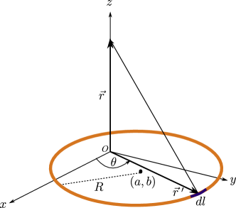
Figure 1: Graphic representation of the considered situation.

so we have

$$\Phi(\vec{r})=\frac{\lambda}{4\pi\epsilon_{0}}\int\frac{dl}{\mid\vec{r}-\vec{r}^{\;{}^{\prime}}\mid}.$$ (2)

Using the parametric equation of a non centered ring given by $x^{\prime}=a+R\cos\theta$ and $y^{\prime}=b+R\sin\theta$, where ($a$,$b$) corresponds to the coordinates of the center of the ring and $0\leq\theta\leq 2\pi$. Therefore $\vec{r}=z\hat{k}$ and $\vec{r}^{\,{}^{\prime}}=(a+R\cos\theta)\hat{\imath}+(b+R\sin\theta)\hat{\jmath}$, so we can obtain the infinitesimal length element by means of

$$dl=\mid d\vec{r}^{\,{}^{\prime}}\mid=\sqrt{(dx^{\prime})^{2}+(dy^{\prime})^{2}}=Rd\theta.$$ (3)

Then, the electrostatic potential in the $z$ axis is given by

$$\Phi(z)=\frac{\lambda}{4\pi\epsilon_{0}}\int_{0}^{2\pi}\frac{R\,d\theta}{\sqrt{a^{2}+b^{2}+R^{2}+z^{2}+2aR\cos\theta+2bR\sin\theta}}$$ (4)

defining $\alpha=a/R$, $\beta=b/R$, $\zeta=z/R$ and $\Lambda=\alpha^{2}+\beta^{2}+\zeta^{2}+1$ we have

$$\Phi(\zeta)=\frac{\lambda}{4\pi\epsilon_{0}}\int_{0}^{2\pi}\frac{d\theta}{\sqrt{\Lambda+2\alpha\cos\theta+2\beta\sin\theta}},$$ (5)

The integral in the equation (5) can be written as [10]

$$I=\int_{0}^{2\pi}\frac{d\theta}{\sqrt{\Lambda+2\alpha\cos\theta+2\beta\sin\theta}}=\int_{-\varphi}^{2\pi-\varphi}\frac{du}{\sqrt{\Lambda+\varepsilon\cos u}}.$$ (6)

The parameters of equation (6) are defined by $\varphi=\arctan(\beta/\alpha)$ and $\varepsilon=2\beta/\sin\varphi=2\sqrt{\alpha^{2}+\beta^{2}}$ and the variable $u=\theta-\varphi$. Using the transformation $u=2\phi$ we can re write the denominator of integrand (6) as

$$(\Lambda+\varepsilon\cos u)^{1/2}=(\Lambda+\varepsilon)^{1/2}\left(1-m\sin^{2}\phi\right)^{1/2},$$ (7)

where $m=2\varepsilon/(\Lambda+\varepsilon)$. So the equation (6) can be written as

$$I=\frac{2}{\sqrt{\Lambda+\varepsilon}}\int_{-\varphi/2}^{\pi-\varphi/2}\frac{d\phi}{\sqrt{1-m\sin^{2}\phi}}.$$ (8)

The solution of the integral (8) is given by the incomplete elliptic integral of the first kind $F(\varphi,m)$ [11]

$$F(\varphi,m)=\int_{0}^{\varphi}(1-m\sin^{2}\phi)^{-1/2}d\phi,$$ (9)

then, the electrostatic potential in $z$ axis is

$$\Phi(\zeta)=\frac{\lambda}{2\pi\epsilon_{0}}\frac{1}{\sqrt{(1+\gamma)^{2}+\zeta^{2}}}\left[F\left(\frac{\varphi}{2},\frac{4\gamma}{(1+\gamma)^{2}+\zeta^{2}}\right)-F\left(-\pi+\frac{\varphi}{2},\frac{4\gamma}{(1+\gamma)^{2}+\zeta^{2}}\right)\right]$$ (10)

where $\gamma=\sqrt{\alpha^{2}+\beta^{2}}$.

Since $F(0,m)=0$ and $F(-\pi,m)=-2K(m)$, where $K(m)$ is the complete elliptic integral of the first kind in terms of the parameter $m$, we can make $\beta=0$ and $\alpha=0$ then $m=0$. Noticing that $K(0)=\pi/2$, we have

$$\Phi(z)=\frac{Q}{4\pi\epsilon_{0}}\frac{1}{\sqrt{R^{2}+z^{2}}},$$ (11)

which is the electrostatic potential in the $z$ axis of a centered ring.

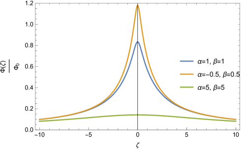
Figure 2: Electrostatic potential $\Phi(z)$ (eq. 10) normalized to the potential in $\Phi(0)=\Phi_{0}$ of a unitary radius ring for different positions of the ring in the plane.

As we can see from the figure 2 the normalized electrostatic potential if the center of the ring moves away form the origin coordinate, the normalized electrostatic potential in the $z$ axis tends to vanish.

If we compare this situation with the electrostatic potential, in the space, of a centered ring [4, 5, 6], we can consider that the ring its displaced a distance $\gamma=\sqrt{\alpha^{2}+\beta^{2}}$ from the origin coordinate $O$. Considering $\gamma$ to lie on the plane of the ring along the $x$ direction, then $\beta=0$ so $\gamma=\alpha=\varrho$, where $\varrho=\rho/R$. Therefore, the electrostatic potential is given by

$$\Phi(\varrho,\zeta)=\frac{\lambda}{2\pi\epsilon_{0}}\frac{2}{\sqrt{(\varrho+1)^{2}+\zeta^{2}}}K\left[\frac{4\varrho}{(1+\varrho)^{2}+\zeta^{2}}\right],$$ (12)

or in terms of $z$

$$\Phi(\rho,z)=\frac{Q}{4\pi^{2}\epsilon_{0}}\frac{2}{\sqrt{(\rho+R)^{2}+z^{2}}}K\left[\frac{4R\rho}{(\rho+R)^{2}+z^{2}}\right].$$ (13)

3 Electric field

As is known, the electric field can be obtained from the potential gradient. In cylindrical coordinates, considering cylindrical symmetry, the electric field is given by

$$\vec{E}=-\vec{\nabla}\Phi(\rho,z)=-\left(\frac{\partial}{\partial\rho}\hat{\rho}+\frac{\partial}{\partial z}\hat{k}\right)\Phi(\rho,z),$$ (14)

however, in order to obtain an expression for the electric field in terms of the coordinates $(\varrho,\zeta)$, we must consider the change of variable $\varrho=\rho/R$ and $\zeta=z/R$ to preserve the dimensions of the electric field, so we have

$$\vec{E}=-\frac{1}{R}\left(\frac{\partial}{\partial\varrho}\hat{\varrho}+\frac{\partial}{\partial\zeta}\hat{k}\right)\Phi(\varrho,\zeta).$$ (15)

As we seen before, the expressions (10) and (12) are analogous, so we can obtain the $(\varrho,\zeta)$ components of the electric field by means of the gradient of equation (12), using the expression (15).

Considering that

$$\frac{dK(k)}{dk}=\frac{E(k)}{k(1-k^{2})}-\frac{K(k)}{k}$$ (16)

and

$$\frac{dE(k)}{dk}=\frac{E(k)-K(k)}{k},$$ (17)

where $E(k)$ is the incomplete elliptic integral of the second kind. After some manipulations, the radial component of the electric field is given by

$$E_{\varrho}= \frac{\lambda}{2\pi\epsilon_{0}R}\frac{1}{\varrho\sqrt{(1+\varrho)^{2}+\zeta^{2}}((\varrho-1)^{2}+\zeta^{2})}$$

$$\times\left\{(\varrho^{2}-1-\zeta^{2})E\left[\frac{4\varrho}{(1+\varrho)^{2}+\zeta^{2}}\right]+((1-\varrho)^{2}+\zeta^{2})K\left[\frac{4\varrho}{(1+\varrho)^{2}+\zeta^{2}}\right]\right\},$$

and the vertical component of the electric field is

$$E_{\zeta}=\frac{\lambda}{2\pi\epsilon_{0}R}\frac{2\zeta}{\sqrt{(1+\varrho)^{2}+\zeta^{2}}((\varrho-1)^{2}+\zeta^{2})}E\left[\frac{4\varrho}{(1+\varrho)^{2}+\zeta^{2}}\right].$$ (19)

From the equations (3) and (19) we can check the cases when $\varrho\to 0$. In this cases we must recover the expression for a centered uniformly charged ring for the vertical component and zero for the radial component of the electric field.

As we can see, the expression (3) can not be evaluated directly in $\varrho=0$ as it presents a $0/0$ behaviour. So we must calculate the limit as $\varrho\to 0$.

Considering (16) and (17), and after some manipulation we have

$$E_{\varrho}= \frac{\lambda}{2\pi\epsilon_{0}R}\frac{1}{\sqrt{(1+\varrho)^{2}+\zeta^{2}}(\varrho^{3}+4\varrho^{4}+5\varrho^{2}(\zeta^{2}-1)-\varrho(1+\zeta^{2})+(1+\zeta^{2})^{2})}$$ (20)

$$\times\left\{((1+\varrho)^{3}+(1+3\varrho)\zeta^{2})E\left[\frac{4\varrho}{(1+\varrho)^{2}+\zeta^{2}}\right]\right.$$

$$\left.+(\varrho-1)(1+\varrho(4+3\varrho)+\zeta^{2})K\left[\frac{4\varrho}{(1+\varrho)^{2}+\zeta^{2}}\right]\right\}.$$

Evaluating the limit $\varrho\to 0$ in the expression (20) and noticing that $E(0)=\pi/2$ and $K(0)=\pi/2$, we ended up with

$$E_{\varrho}=0.$$

On the other hand, we can calculate directly the electric field in the vertical component for $\varrho=0$ in the expression (19)

$$E_{\zeta}=\frac{\lambda}{2\epsilon_{0}R}\frac{\zeta}{(1+\zeta^{2})^{3/2}},$$ (21)

as $\zeta=z/R$ and $\lambda=Q/2\pi R$ we obtain the well known expression for the electric field of an centered uniformly charged ring along the symmetry axis

$$E_{z}=\frac{Q}{4\pi\epsilon_{0}}\frac{z}{(R^{2}+z^{2})^{3/2}}.$$ (22)

4 Conclusions

It has been presented a general method to obtain the electrostatic potential using an adequate parametrization of a loop through the use of elliptic integrals. From this result, it could recover the expressions of the electrostatic potential and electric field on the symmetry axis of a centered ring. Finally, the obtained results agree with the calculations of the electrostatic potential off the symmetry axis of a centered ring and are useful as a pedagogical exercise for to students can explore special functions in an electromagnetism problem.

References

References

• [1] R. A. Serway and J. W. Jewett Physics for Scientists and Engineers, Brooks Cole 2015.
• [2] H. D. Young, R. A. Freedman Sears and Zemansky’s university physics: with modern physics, Pearson Addison-Wesley 2008.
• [3] P. A. Tipler and G. Mosca Physics for scientist and engineers with modern Physics, W. H. Freeman 2007.
• [4] R. H. Good, Elliptic integrals, the forgotten functions, Eur. J. Phys. 22 (2001) 119–126.
• [5] O. Ciftja, A. Babineaux and N. Hafeez, The electrostatic potential of a uniformly charged ring, Eur. J. Phys. 30 (2009) 623–627.
• [6] H. Noh, Electrostatic Potential of a Charged Ring: Applications to Elliptic Integral Identities, Journal of the Korean Physical Society, 71 (2017) 37–41.
• [7] O. Ciftja and I. Hysi, The electrostatic potential of a uniformly charged disk as the source of novel mathematical identities, Applied Mathematics Letters, 24 (2011) 1919–1923.
• [8] V. Bochko and Z. K. Silagadze, On the electrostatic potential and electric field of a uniformly charged disk, Eur. J. Phys. 41 (2020) 045201.
• [9] John. D. Jackson 1999, Classical Electrodynamics, Third edition, John Wiley, p. 30.
• [10] I. S. Gradshteyn and I. M. Ryzhik, 20017, Table of integrals, series and products, Seven edition, Academic Press, p. 174.
• [11] M. Abramowitz and I. A. Stegun, 1964 Handbook of Mathematical Functions, Dover Publications, p. 589.