Comparison of Random Sampling and Heuristic Optimization-Based Methods for Determining the Flexibility Potential at Vertical System Interconnections

Abstract

In order to prevent conflicting or counteracting use of flexibility options, the coordination between distribution system operator and transmission system operator has to be strengthened. For this purpose, methods for the standardized description and identification of the aggregated flexibility potential of distribution grids are developed. Approaches for identifying the feasible operation region (FOR) of distribution grids can be categorized into two main classes: Random sampling/stochastic approaches and optimization-based approaches. While the former have the advantage of working in real-world scenarios where no full grid models exist, when relying on naiv̈e sampling strategies, they suffer from poor coverage of the edges of the FOR due to convoluted distributions. In this paper, we tackle the problem from two different sides. First, we present a random sampling approach which mitigates the convolution problem by drawing sample values from a multivariate Dirichlet distribution. Second, we come up with a hybrid approach which solves the underlying optimal power flow problems of the optimization-based approach by means of a stochastic evolutionary optimization algorithm codenamed REvol. By means of synthetic feeders, we compare the two proposed FOR identification methods with regard to how well the FOR is covered and number of power flow calculations required.

I Introduction

The increasing share of distributed energy resources (DERs) in the electrical energy system leads to new challenges for both, transmission system operators (TSOs) and distribution system operators (DSOs). Flexible ancillary services for congestion management, voltage maintenance or power balancing, so far mostly provided by large scale thermal power plants directly connected to the transmission grid (TG), increasingly have to be provided by DERs connected to the distribution grid (DG). Thus, DGs evolve from formerly mostly passive systems to active distribution grids (ADGs) that contain a variety of controllable components interconnected via communication infrastructure and whose dynamic behavior is characterized by higher variability of vertical power flows and greater simultaneity factors.

TSO-DSO coordination is an important topic which has been pushed by ENTSO/̄E during the last years [1, 2, 3, 4]. Coordination between grid operators has to be strengthened to prevent conflicting or counteracting use of flexibility options [5]. To reduce complexity for TSOs at the TSO/DSO interface and to enable TSOs to consider the flexibility potential of DGs in its operational management and optimization processes, methods are needed which allow for the determination and standardized representation of the aggregated flexibility potential of DGs.

The aggregated flexibility potential of a DG can be described as region in the PQ-plane that is made up from the set of feasible interconnection power flows (IPFs) [6]. Thereby, feasible IPFs are IPFs which can be realized by using the flexibilities of controllable DERs and controllable grid components such as on-load tap changer (OLTC) transformers in compliance with grid constraints i.e., voltage limits and maximum line currents.

In the literature, there are various concepts to determine the FOR of DGs. They can be categorized into two main classes: Random sampling/stochastic approaches and optimization-based approaches.

For random sampling approaches in its simplest form, the general procedure is such that a set of random control scenarios is generated by assigning set-values from a uniform distribution to each controllable unit. By means of load flow calculations the resulting IPFs are determined for each control scenario and classified into feasible IPFs (no grid constraints are violated) and non-feasible IPFs (at least one grid constraint is violated). The resulting point cloud of feasible IPFs in the PQ-plane serves as stencil for the FOR [6]. A problem that comes with this approach is that drawing set-values from independent uniform distributions leads to an unfavorable distribution of the resulting IPFs in the PQ-plane and extreme points on the margins of the FOR are not captured well [7].

This is where optimization-based methods come into play. The basic idea behind these methods is not to randomly sample IPFs but systematically identify marginal IPFs by solving a series of optimal power flow (OPF) problems [8]. In addition to better coverage of the FOR, optimization-based approaches have the advantage of higher computational efficiency. An important drawback is however that, except for approaches which solve the OPF heuristically, solving the underlying OPF requires an explicit grid model [9]. On the other hand, the only heuristic approach published so far suffers from poor automatability as it relies on manual tweaking of hyperparameters [10].

In practice, considering the huge size of DGs, data related to the grid topology (asset data, operating equipment, etc.) usually does not cover the whole grid [11], which complicates parametrization of explicit grid models. In such circumstances, black-box machine learning (ML) models trained on measurement data provided by current smart meters can be an alternative to physics-based, explicit grid models [12]. Therefore, we argue that it is worthwhile to research FOR determination techniques, which are compatible with black-box grid models. In this paper, we tackle the problem from two different sides. As we have detailed the convolution problem previously [7], we now show a solution approach. In this vein, we provide a comparison between a random sampling method more suited to the problem, as well as a heuristic as informed search method. First, we present our random sampling approach which mitigates the convolution problem by drawing sample values from a multivariate Dirichlet distribution. Second, we introduce a hybrid approach which solves the underlying OPF problems of the optimization-based approach heuristically by means of the evolutionary optimization algorithm REvol [13]. To show automatability, in contrast to [10], we do no manual tweaking of hyperparameters. Instead, parameter optimization is done via random search. Furthermore, we do not make problem-specific adjustments to the optimization algorithm.

The remainder of the paper is structured as follows: A survey on existing approaches (random sampling and optimization-based) and the contribution of this paper are given in section II. Next, in section III, the construction of a series of synthetic feeders with increasing number of nodes is explained. These feeders are used for comparison and evaluation of our proposed FOR determination techniques. In the subsequent sections IV and V, we present our stochastic approach based on sampling from a Dirichlet distribution and our hybrid approach using REvol for solving the series of OPF problems. In this context, we additionally discuss how the parameter tuning is performed and introduce the Jaccard index as a measure for comparing FORs. After this, in section VI, we present and discuss our results. Finally, in section VII, the paper is summarized and the conclusion—along with a brief outline of future work—is given.

II Related work and contribution of this paper

As outlined in the introduction, relevant literature can be grouped into two main categories: Random sampling/stochastic and optimization-based approaches for exploring the FOR of DGs. The following two subsections are mainly taken from [7]. In [7], we motivate work presented in this paper by pointing out the convolution problem when sampling from uniform distributions.

II-A Random sampling approaches

[14] are the first to come up with the idea of estimating the flexibility range in each primary substation node to inform the TSO about the technically feasible aggregated flexibility of DGs. In order to enable the TSO to perform a cost/benefit evaluation, they also include the costs associated with adjusting the originally planned operating point of flexible resources in their algorithm. In the paper two variants of a Monte Carlo simulation approach are presented, which differ in the assignment of set-values to the flexible resources. While in the first approach independent random set-values for changing active and reactive power injection are associated to each flexible resource, in the second approach a negative correlation of one between generation and load at the same bus was considered. In a direct comparison of the two presented approaches, the approach with negative correlation between generation and load at the same bus performs better and results in a wider flexibility range and lower flexibility costs with a smaller sample size. Nevertheless, even with this approach, the capability to find marginal points in the FOR is limited. Therefore, in the outlook the authors suggest the formulation of an optimization problem in order to overcome the limitations of the Monte Carlo simulation approach, increasing the capability to find extreme points of the FOR and reducing the computational effort. In [8], which is discussed in the next subsection, the authors take up this idea again.

[6] extend in their paper the methodology presented by [14]. First, they describe an approach to approximate the FOR of an ADG for a particular point in time assuming that all influencing factors are known. For this, they use the first approach of [14] for sampling IPFs (the one that does not consider correlations). That is, random control scenarios are generated by assigning set-values from independent uniform distributions to all controllable units. In contrast to [14], no cost values are calculated for the resulting IPFs. Instead, for describing the numerically computed FOR with sparse data, the region is approximated with a polygon in the complex plane. In addition, a probabilistic approach to assess in advance the flexibility associated to an ADG that will be available in a future time interval under consideration of forecasts which are subject to uncertainty is proposed. The authors mention that for practical usage the computation time for both approaches has to be significantly reduced. However, the problem of unfavorable distribution of the resulting IPF point cloud, when drawing control scenarios from independent uniform distributions, which is a mayor factor for the low computational efficiency, is not discussed.

When research presented in this paper was already advanced, [15] came up with advanced random sampling approaches. They show that, when focusing the vertices of the flexibility chart of flexibility providing units during sampling, FOR coverage can be dramatically improved in comparison to the naiv̈e sampling. On top of that, they present a comparison of OPF-based and random sampling approaches, whose results show that with their improved sampling strategies both approaches are capable of assessing the FOR of radial distribution grids but for grids with large number of buses OPF-based methods are still better suited.

II-B Optimization-based approaches

[8] address the main limitation of their sampling-based approach in [14], namely estimating extreme points in the FOR. To this end, they propose a methodology which is based on formulating an optimization problem with below-mentioned objective function, whose maximization for different ratios of $\alpha$ and $\beta$ allows to capture the perimeter of the flexibility area.

$$\alpha\>P_{\mathit{DSO}\rightarrow\mathit{TSO}}+\beta\>Q_{\mathit{DSO}\rightarrow\mathit{TSO}}$$ (1)

where $P_{\mathit{DSO}\rightarrow\mathit{TSO}}$ and $Q_{\mathit{DSO}\rightarrow\mathit{TSO}}$ are the active and reactive power injections at the TSO-DSO boundary nodes. [8] work out that the underlying optimization problem represents an OPF problem. Due to its robust characteristics they use the primal-dual, a variant of the interior point methods to solve it. The methodology was evaluated in simulation and validated in real field-tests on MV distribution networks in France. The comparison of simulation results with the random sampling algorithm in [14] shows the superiority of the optimization-based approach by illustrating its capability to identify a larger flexibility area and to do it within a shorter computing time.

[16] propose the concept of active-reactive power (PQ) chart, which characterizes the short-term flexibility capability of active distribution networks to provide ancillary services to TSO. To support this concept, an AC optimal power flow-based methodology to generate PQ capability charts of desired granularity is proposed and illustrated in a modified 34-bus distribution grid.

[9] present a linear optimization model for the aggregation of active and reactive power flexibility of distribution grids at a TSO-DSO interconnection point. The power flow equations are linearized by using the Jacobian matrix of the Newton-Raphson algorithm. The model is complemented with non-rectangular linear representations of typical flexibility providing units, increasing the accuracy of the distribution grid aggregation. The obtained linear programming system allows a considerable reduction of the required computing time for the process. At the same time, it maintains the accuracy of the power flow calculations and increases the stability of the search algorithm while considering large grid models.

[17] present a method to compute reduced and aggregated distribution grid representations that provide an interface in the form of active and reactive power (PQ) capability areas to improve TSO-DSO interactions. Based on a lossless linear power flow approximation they derive polyhedral sets to determine a reduced PQ operating region capturing all voltage magnitude and branch power flow constraints of the DG. While approximation errors are reasonable, especially for low voltage grids, computational complexity is significantly reduced with this method.

[10] provide a detailed survey on stochastic and optimization based methods for the determination of the FOR. They come up with a comparison of different FOR determination methods with regard to quality of results and computation time. For their comparison they use the Cigré medium voltage test system. On top of that, they present a particle swarm optimization (PSO) based method for FOR determination.

Contributions of this paper

In summary, it can be stated that optimization-based approaches show high computational efficiency with good coverage of the FOR. However, methods used for solving the underlying OPF problem rely—except for heuristic approaches—on explicit grid models of the DG, which must be parametrized with grid topology data often not available in practice. At the same time, the only heuristic approach presented so far, suffers from poor automatability due to manual tweaking of hyperparameters [10]. Random sampling approaches, on the other hand, do not require explicit grid modeling and are compatible with black-box grid models, but suffer from low computational efficiency and poor coverage of peripheral regions of the FOR, when using conventional sampling strategies.

In this paper, we tackle the problem from two different sides. First, we present a random sampling approach which mitigates the convolution problem. In a two-stage procedure, we start with drawing set-values from a uniform distribution for the aggregated active and reactive power of the flexible units (inverter-connected batteries in our case). In a second step, the previously determined set-values for the aggregated power are distributed to the individual units. For this, the Dirichlet distribution is used. Here, we make use of the property that the sum of the entries of the random vectors generated from the multivariate Dirichlet distribution is always one.

Our second approach is to make the optimization-based approach black-box model compatible by solving the underlying OPF problem heuristically with the evolutionary optimization algorithm REvol [13]. To show automatability, we use randomized search for hyperparameter tuning. As score for parameter optimization we take the Jaccard index to measure similarity between FORs determined by REvol with varying parameter combinations and a benchmark FOR, which is generated by applying the Dirichlet sampling. To get close to the actual FOR, a large sample size ($100\,000$ sample elements) is used for creating the benchmark FOR.

III Synthetic benchmark feeders and comparison scenario

Evaluation and comparison of the FOR identification methods presented in this paper are done on the basis of a series of synthetic $0.4\text{\,}\mathrm{k}\mathrm{V}$ feeders as shown in Figure 1. Construction of the synthetic feeders is explained in more detail in [7]. The feeders are characterized by an increasing number of nodes. In order to better evaluate how an increasing number of nodes affects the investigated FOR determination methods, both, the total installed power and the mean transformer-node distance are chosen equal for all feeders. This results in similar, easily comparable FORs regardless of the number of nodes.

Figure 1: Synthetic $0.4\text{\,}\mathrm{k}\mathrm{V}$ feeders

For our experiments, we have constructed four synthetic $0.4\text{\,}\mathrm{k}\mathrm{V}$ feeders. The feeders differ in the number of nodes $N^{i}$, which has been set to $1$, $3$, $9$ or $27$ respectively. To get similar FORs for all feeders, line length $l^{i}_{l}$ and feeder length $l^{i}_{f}$ have then been calculated in such a way, that the mean transformer-node distance is equal for all feeders. The resulting line parameters are shown in Table I. Formulas for calculating the line lengths, can be found in [7]. There is one DER connected to each node and the installed power $P^{i}_{inst,DERs}$ is distributed evenly among the DERs. To be able to cover the entire flexibility area of the feeders including their border areas where voltage band violations and/or line overloadings can be observed, all DERs are inverter-connected battery storages because they offer maximum flexibility with regard to both, active and reactive power provision. The dimensioning of the inverters has been chosen in such a way that a power factor $\cos{\phi}$ of 0.9 inductive can be kept, when the maximum active power is delivered: Values for the technical parameters of the four feeders including connected DERs are listed in Table I.

Table I: Configuration of the synthetic feeders

# DERs	$\mathrm{P_{inst,DER_{j}}}$ (kW)	$\mathrm{|S|_{max,DER_{j}}}$ (kVA)	Feeder Length (m)	Line Length (m)	Line Type	Voltage Band (pu)	Trafo Type
1	200.0	222.2	400	400	NAYY 4x150 SE	0.9–1.1	0.4 MVA 20/0.4 kV
3	66.7	74.1	600	200	NAYY 4x150 SE	0.9–1.1	0.4 MVA 20/0.4 kV
9	22.2	24.7	720	80	NAYY 4x150 SE	0.9–1.1	0.4 MVA 20/0.4 kV
27	7.4	8.2	771	29	NAYY 4x150 SE	0.9–1.1	0.4 MVA 20/0.4 kV

IV Two-stage random sampling approach with sampling from Dirichlet distribution

To mitigate the problem of convoluted distributions when using classical sampling strategies, as it was pointed out in [7], we propose a two-stage procedure. It is motivated by the following basic consideration: During sampling, the FOR should be covered evenly. As IPFs are mostly made up of the sum of power injections of connected DERs (grid losses are comparatively small), it is reasonable to draw set-values for the aggregated power of connected DERs in a first step and then distribute them randomly to the individual units. To do so, we need an appropriate distribution which allows for sampling random vectors with given sum (to match the set value for the aggregated power drawn in the first step). As it has exactly this property, this is where the Dirichlet distribution $\operatorname{Dir}(\boldsymbol{\alpha})$ comes into play. It is a continuous multivariate probability distribution parameterized by a vector $\boldsymbol{\alpha}$ of positive reals, which controls the concentration of the distribution:

$$\operatorname{Dir}(\boldsymbol{\alpha})=f\left(x_{1},\ldots,x_{K};\alpha_{1},\ldots,\alpha_{K}\right)$$ (2)

where:

$$\sum_{i=1}^{K}x_{i}=1\mbox{ and }x_{i}\geq 0\mbox{ for all }i\in\{1,\dots,K\}$$ (3)

with $K$ indicating the order of the multivariate distribution. For the details regarding the Dirichlet distribution, please refer to statistics text books e.g., [18].

The power set-values for the individual units generated by means of the Dirichlet distribution are not distributed uniformly. The shape of the distribution can be manipulated via the $\boldsymbol{\alpha}$ parameter. With $\alpha_{i}=1$ for all $i\in\{1,\dots,K\}$, the distribution of the individual set-values is biased towards low power values. During an initial experimenting phase, by trial and error, $\alpha_{i}=1.2$ for all $i\in\{1,\dots,K\}$ has turned out to be good. Systematic optimization of $\boldsymbol{\alpha}$ is part of future work.

There is another factor biasing the distribution of IPFs. Due to the fact, that the random power set-values for the individual units generated by means of the Dirichlet distribution are not all in the power range that can be realized by the individual units and set-values beyond the limits are clipped by our simulations. This would result in an accumulation of IPFs at the upper edge of the FOR.

To reduce the aforementioned distortions, before applying the normalized set-values to our simulation environment, we split the sample in four subsets of equal size. The first subset remains unchanged, for the second subset, normalized active power values $\boldsymbol{p_{n}}$ are transformed with $\boldsymbol{p_{n}^{\prime}=-p_{n}^{\prime}+1}$, for the third subset, the transformation is done to the reactive power set-values $\boldsymbol{q_{n}}$ ($\boldsymbol{q_{n}^{\prime}=-q_{n}+1}$). Finally, with the fourth subset, the transformation is applied to both, active and reactive power set-values.

We proceed in such a way, that we calculate the absolute active and reactive power set-values from the normalized ones generated during sampling. After assigning these values to the DERs, we step the rudimentary inverter simulators via which all batteries are connected to the synthetic feeders. The inverter models monitor that the maximum current of the inverters is not exceeded. In case the provided set point is not compatible with the current limits of the inverter, it is operated at an operating point which is as close as possible to the preset, but still complies with the current constraint. The power values returned from the inverter simulators are than passed to the pandapower library [19] which is used for calculating the power flows. This way, we generate a sample of size $10\,000$ for each feeder.

Following this, the sample elements are first classified with regard to their adherence to grid constraints and in case of non-adherence with regard to the type of grid constraint violation (i.e., voltage band violation, line overload, or both). In the final step, we compute the convex hull around the IPFs which do not violate any constraints and thus make up the FOR.

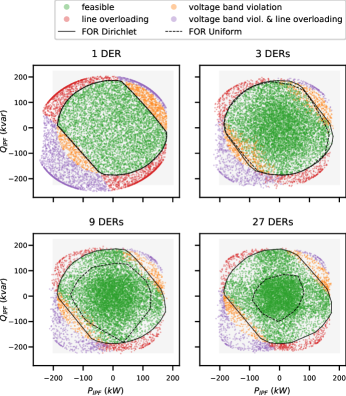
Figure 2: Results of sampling from Dirichlet distribution ($10\,000$ sample elements) classified by feasibility with regard to grid constraints (voltage band limits and max. line loading); black solid line indicates the resulting FOR; black dotted line indicates FOR when sampling from uniform distribution with same sample size

The resulting FORs for feeders with increasing number of nodes are shown in Figure 2. The border of the FOR is marked by the solid black line in each case. For comparison, the dashed lines define the FORs which result from sampling from a uniform distribution. It can be seen from the plots that with the Dirichlet approach the identified FOR is approximately the same for all tested feeders. A collapsing FOR, as observed with the uniform sampling approach (dotted lines), does not occur. This indicates that the folding problem, we pointed out in [7], is mitigated with the procedure proposed here.

Nevertheless, it can be easily seen, that even with the Dirichlet approach, the FOR is not evenly covered. As the number of nodes increases, clusters are formed around the coordinate origin and along the axes. This is particularly problematic in that fewer points are sampled in the interesting areas in the first and third quadrant, where due to voltage band violations the density of valid IPFs decreases anyway. The reason probably lies in the transformation of the data along the main axes, which is motivated by mitigating the bias caused by clipping of set-values beyond the power limits of the DERs. A more suitable data transformation and an optimized selection of the $\boldsymbol{\alpha}$ parameter of the Dirichlet distribution could remedy this and offer potential for future work.

We use the two-stage Dirichlet approach presented in this section to generate the benchmark FOR for the parameter tuning of the optimization-based approach which will be introduced in the next section. In contrast to the results presented here, to get as close as possible to the actual FOR, we increase the sample size from $10\,000$ to $100\,000$.

V Optimization-based approach with multipart evolutionary algorithm REvol

Metaheuristics are a common tool in the field of electric power system optimization and have been used to solve various optimization problems regarding system planning and operation (see [20]). In [10] for the first time a metaheuristic was used in the context of FOR determination. Due to its popularity in solving OPF problems, PSO was applied. For improved performance, in [10] the PSO is tailored to the FOR identification problem and hyperparameters are tweaked manually. Because automation suffers from that, in this paper we choose a different approach and dispense with problem specific customization of the applied metaheuristic and do automated hyperparameter tuning by means of the randomized search facility provided by the Python machine learning framework Scikit-learn [21]. Due to its superior performance compared to PSO on other tasks (training of Artificial Neural Networks (ANNs) for time series prediction), in this paper we give REvol a try in optimization based FOR identification. REvol was introduced in [13]. Comparison with PSO regarding training of ANNs can be found in [22]. The following statements are taken in abbreviated form from [22] and can be read there in detail.

V-A REvol basics

REvol employs an approach similar to the classic evolutionary algorithms in that it defines a number of individuals that live in a population. In contrast to the classical approach, an individual consists of two vectors: A parameter and a scatter vector, each with the same size. While the parameter vector represents a solution candidate for the problem at hand, in our case normalized active and reactive power set-values for each battery connected to the feeder, each component of the scatter vector limits the variability of the corresponding parameter vector’s component. Also, the evolution process is basically the same as for other evolutionary algorithms: Until the number of iterations reaches a predefined maximum, the algorithm generates a new individual, uses a fitness function to evaluate it, and possibly enhances the population with it. However, when it comes to the creation of new individuals REvol has two distinctive features that set it apart from the classic approach:

• The current rate of success

• The implicit gradient information

The current rate of success influences the spread, i.e., the area within which a new individual can potentially be placed. By increasing the spread when the current notion of success is greater then the target success, this helps to escape local minima. In order to avoid fluctuations in the success variable, it is dynamically averaged over a fixed number of iterations, represented by the user supplied variable T. The averaging is done by a time-discrete PT1 element:

$$pt1(y,u,t)=\begin{cases}u&\text{if }t=0\\ y+\frac{u-y}{t}&\text{otherwise}\end{cases}$$ (4)

with $t=T$, except for the initial iteration with $t=0$.

The second factor influencing reproduction, is the gradient information. The area within which new individuals can be placed does not feature a uniform probability density function (PDF). Instead, the placement of the two individuals chosen relative to each other is used to calculate the implicit gradient, i.e., the direction within which a newly generated individual must be placed with a high probability in order to reach the minimum. These two factors carefully balance each other: Putting a strong emphasis on the implicit gradient information would turn the multi-part evolutionary strategy into a ‘poor man’s gradient decent, whereas a high influence of the dynamic reproduction probability density spread will make the algorithm lose its orientation. This is for providing a basic understanding of the algorithm. For the technical details, please refer to [13] and [22].

V-B Sampling strategy and optimization problem

Optimization-based methods for determining the FOR are based on systematically identifying boundary points of the FOR, where the identification of each boundary point represents an optimization problem. At this point, it is important to emphasize that optimization-based approaches are characterized by two important features. First, the systematics which is used to determine the boundary points. In literature, this is also referred to as sampling strategy [10]. The sampling strategy specifies the rules by means of which a series of optimization problems is constructed for systematically determining the FOR. The other important feature characterizing optimization-based FOR identification techniques, is how the resulting series of optimization problems is actually solved, i.e. which optimization method is applied. In this paper, the focus is on the latter. Therefore, a simple sampling strategy is applied, whose basic function is explained in the next paragraph. For a detailed overview of sampling strategies, please refer to [10].

The sampling strategy used for the experiments in this paper is based on solving the optimization problem in Equation 5 for different ratios of $\alpha$ and $\beta$.

$$\max(\alpha\>P_{\mathit{DSO}\rightarrow\mathit{TSO}}+\beta\>Q_{\mathit{DSO}\rightarrow\mathit{TSO}})$$ (5)

where $P_{\mathit{DSO}\rightarrow\mathit{TSO}}$ and $Q_{\mathit{DSO}\rightarrow\mathit{TSO}}$ are the active and reactive power injections at the TSO-DSO boundary nodes. Decision variables are the active and reactive power set points for the connected DERs $P_{set,DER_{j}}$ and $Q_{set,DER_{j}}$. The optimization problem is subject to compliance with grid constraints, which are defined by the minimum and maximum voltage limits, the maximum thermal current limits of the lines and the rated load of the transformer. For our experiments, we determine eight boundary points with:

$$\begin{split}(\alpha,\beta)\in[&(1,0),(1,1),(0,1),(-1,1),\\ &(-1,0),(-1,-1),(-1,0),(1,-1)]\end{split}$$ (6)

V-C Optimization process and restrictions vector

When evaluating individuals during the optimization process, we proceed in the same way as we do with the random sampling based approach in the previous section. However, this time normalized active and reactive power set-values are provided in form of the individual’s parameter vector to the simulation. Again, before calculating the power flow with the pandapower library [19], the inverter simulation model ensures adherence to inverter constraints and updates the parameter vector accordingly. Here, it is important to mention that besides the restrictions vector, which will be introduced in the next paragraph, the updated parameter vector is returned to REvol. It is therefore ensured that all individuals comply with inverter constraints and thus inverter constraint are omitted in the restrictions vector.

procedure isBetterThan($indiv0,indiv1$)

     for $i\leftarrow 1$ to $indiv0.restr.length$ do

         if $(indiv0.restr[i]<indiv1.restr[i])$ then

              return $true$

         else if $(indiv0.restr[i]>indiv1.restr[i])$ then

              return $false$

         end if

     end for

     if $(indiv0.restr[0]>indiv1.restr[i])$ then

         return $true$

     else

         return $false$

     end if

end procedure

Algorithm 1 Comparison operator

REvol uses the restrictions vector for comparison of individuals. Comparison is done when calculating the current rate of success mentioned before and when determining the elite. The elite is composed of the fittest individuals of the population. It plays a role when selecting the parent individuals for the next generation—one individual from the elite and one from the general population are chosen as parent individuals by the algorithm. The restrictions vector has three entries: The first entry holds the individuals fitness, calculated according to Equation 5. In further entries, grid constraint violations are considered—the second entry holds the largest voltage band violation, the third entry the highest exceedance of the line current limits. The comparison operator isBetterThan$(indiv0,indiv1)$ is shown in Algorithm 1. From the pseudocode, it can be seen that small or no grid constraint violations have the highest priority during comparison. Only if both individuals do not have any or the same grid constraint violations, the individual with the higher fitness value is evaluated as better.

V-D Hyperparameter search

Like most metaheuristics, REvol has a number of hyperparameters. They are listed in Table II. To find suitable values for these parameters, parameter search is performed with the randomized search facility provided by the Python machine learning framework Scikit-learn [21]. For comparing the quality of different parameter combinations, an appropriate metric or score is required which indicates how well the actual FOR is reassembled depending on the parameter selection. We use the Jaccard index for this purpose. The Jaccard index is a statistic for measuring the similarity of sample sets and is defined as the size of the intersection divided by the size of the union of the sample sets:

$$J(A,B)={{|A\cap B|}\over{|A\cup B|}}.$$ (7)

The reference FOR is determined according to the two-stage Dirichlet approach presented in Section IV. To get close to the actual FOR, a large sample size of $100\,000$ is chosen for that purpose. It is important to mention, that the parameter search is not done for each individual feeder presented in Section III. Instead, we limit the parameter search to the $9$ node feeder and assume that the REvol parameters found for this feeder are also suitable for other networks. A total of $210$ parameter settings are sampled from uniform distributions. To account for the stochastic nature of the algorithm, three runs are performed for each parameter selection. The range from which the individual parameters are sampled and the best parameter combination detected, can be taken from Table II. For the best parameter combination, the Jaccard index results in a mean value of $0.923$ with a standard deviation of $0.0061$. An exact coverage of the benchmark FOR would result in a Jaccard index of $1.0$. Since we determine only eight boundary points, this value cannot be reached, of course.

Table II: REvol parameter selection

Parameter	Range	Best
population size	$20$–$40$	$37$
elite size	$2$–$5$	$3$
max. epochs	$500$–$20\,000$	$16\,245$
max. no success epochs	$20$–$20\,000$	$9281$
T	$10$–$20\,000$	$5338$
start time to live	$80$–$20\,000$	$763$
gradient weight	$0.0$–$3.0$	$2.87$
success weight	$0.0$–$3.0$	$2.18$
target success	$0.1$–$0.4$	$0.29$
max. scatter relative	$0.2$–$3.0$	$1.74$

VI Evaluation and comparison of proposed FOR identification techniques

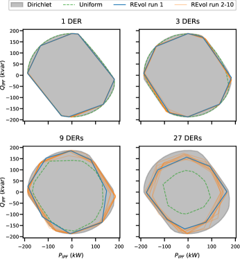
Figure 3: Comparison of FORs resulting from different FOR identification techniques (random sampling Dirichlet, random sampling Uniform and optimization-based REvol) for feeders with increasing number of nodes

The plots in Figure 3 show the FORs resulting from the random sampling Dirichlet and the optimization-based REvol approach in comparison. For a better understanding of the results, the plots also include the FORs that can be obtained when sampling from uniform distributions. The comparison was performed on the basis of the synthetic feeders described in Section III. The benchmark feeders are characterized by an increasing number of nodes and connected DERs. This allows to investigate how well the proposed FOR identification techniques cope with increasing dimensionality of the search space. For the Dirichlet approach and when sampling from uniform distributions, the sample size was set to $100\,000$. The REvol parameters are allocated with the best parameters found during parameter search. The exact values can be taken from the third column in Table II. To account for the stochastic nature of REvol and to be able to evaluate the reliability of the procedure, $10$ runs have been performed with the REvol approach. Because the borders of the FORs resulting from different runs are difficult to distinguish in the plots, the first run is highlighted with its own color (blue solid line). The two upper plots in Figure 3 show that for feeders with small number of DERs, the REvol approach delivers good and reliable results. Apart from few exceptions in the $3$ DERs case, the detected boundary points lie on the border of the FOR determined with the Dirichlet approach or even slightly outside, which shows that the Dirichlet approach does not completely capture the actual FOR either. Nevertheless, parts of the FOR are not covered with the REvol based approach. But this is mainly due to the basic sampling method and the limitation to eight boundary points. From the two plots below, it can be seen that the solution quality with REvol is still decent in comparison to the random sampling from uniform distributions but decreases with increasing number of nodes. Especially with the $27$ nodes feeder, some boundary points of some runs are well within the FOR determined with the two-stage Dirichlet random sampling approach. Moreover, from the increasing spread of the orange lines in Figure 3 it can be taken that the variance of the identified FORs increases with increasing number of nodes.

The runtime of both, the Dirichlet and the REvol approach is dominated by the power flow calculations which are performed when evaluating sample elements and fitness function respectively. Thus, the number of load flow calculations is a good indicator for runtime comparison. The Dirichlet approach also performs better in this respect. The evaluation of the REvol optimization processes for each boundary point in each run and each feeder has revealed that in each case the maximum number of $16\,245$ epochs were cycled through. With eight boundary points, this results in about $130\,000$ power flow calculations compared to $100\,000$ power flow calculations with the two-stage Dirichlet approach and when sampling from uniform distributions.

VII Conclusion and Future Work

Aggregating the flexibility potential of DGs is an important prerequisite for effective TSO-DSO coordination in electric power systems with high share of generation located in the DG level. In this paper, we first gave an overview of existing flexibility aggregation methods and categorized them in terms of whether they are random sampling/stochastic or optimization-based. Following this, we discussed the strengths and weaknesses of both approaches (stochastic and optimization-based) and motivated the investigation of black-box grid model compatible FOR determination techniques. Towards this, we presented an improved random sampling based approach which mitigates the convolution problem by drawing sample values from a multivariate Dirichlet distribution. Second, we made the optimization-based approach black-box compatible by applying the heuristic evolutionary algorithm REVol for solving the underlying OPF problem. To show automatability, we used randomized search for hyperparameter selection.

Comparison of the two presented approaches has shown that both provide decent coverage of the FOR, whereby the random sampling Dirichlet approach produces overall better results at lower runtimes. With the REvol approach, however, we still see potential for improvement with regard to the runtime by considering the runtime as a second factor during parameter search besides FOR coverage. Furthermore, in future work we want to investigate if the total number of required fitness function evaluations can be reduced when sampling the border of the FOR in one run by dynamically adapting the underlying fitness function. In addition to improving the runtime of the REvol approach, in future work we will compare it with other metaheuristics such as PSO and Covariance Matrix Adaption Evolution Strategy (CMA-ES) on a more realistic benchmark grid.

References

- [1] ENTSO-E “General Guidelines for Reinforcing the Cooperation between TSO and DSO”, 2015
- [2] ENTSO-E “Towards Smarter Grids: Developing TSO and DSO Roles and Interactions for the Benefit of Consumers”, 2015
- [3] ENTSO-E “Distributed Flexibility and the Value of TSO / DSO Cooperation – Fostering Active Customer Participation to Value Their Services on the Market – An ENTSO-E Position”, 2017
- [4] ENTSO-E “TSO-DSO Report – An Integrated Approach to Active System Management with the Focus on TSO-DSO Coordination in Congestion Management and Balancing”, 2019
- [5] Marcel Sarstedt et al. “Standardized Evaluation of Multi-Level Grid Control Strategies for Future Converter-Dominated Electric Energy Systems” In at - Automatisierungstechnik 67.11, 2019, pp. 936–957
- [6] D. Mayorga Gonzalez et al. “Determination of the Time-Dependent Flexibility of Active Distribution Networks to Control Their TSO-DSO Interconnection Power Flow” In 2018 Power Systems Computation Conference (PSCC) Dublin, Ireland: IEEE, 2018, pp. 1–8
- [7] Johannes Gerster et al. “Pointing out the Convolution Problem of Stochastic Aggregation Methods for the Determination of Flexibility Potentials at Vertical System Interconnections”, 2021 arXiv:2102.03430 [eess.SY]
- [8] Joao Silva et al. “Estimating the Active and Reactive Power Flexibility Area at the TSO-DSO Interface” In IEEE Transactions on Power Systems 33.5, 2018, pp. 4741–4750
- [9] Daniel A. Contreras and Krzysztof Rudion “Improved Assessment of the Flexibility Range of Distribution Grids Using Linear Optimization” In 2018 Power Systems Computation Conference (PSCC) Dublin, Ireland: IEEE, 2018, pp. 1–7
- [10] Marcel Sarstedt et al. “Survey and Comparison of Optimization-Based Aggregation Methods for the Determination of the Flexibility Potentials at Vertical System Interconnections” In Energies 14.3, 2021
- [11] Ravindra Singh, Efthymios Manitsas, Bikash C Pal and Goran Strbac “A Recursive Bayesian Approach for Identification of Network Configuration Changes in Distribution System State Estimation” In IEEE Transactions on Power Systems 25.3, 2010, pp. 1329–1336
- [12] Pedro Barbeiro et al. “State Estimation in Distribution Smart Grids Using Autoencoders” In IEEE 8th International Power Engineering and Optimization Conference (PEOCO2014), 2014, pp. 358–363
- [13] Eric MSP Veith, Bernd Steinbach and Martin Ruppert “An Evolutionary Training Algorithm for Artificial Neural Networks with Dynamic Offspring Spread and Implicit Gradient Information”, 2014
- [14] M. Heleno et al. “Estimation of the Flexibility Range in the Transmission-Distribution Boundary” In 2015 IEEE Eindhoven PowerTech Eindhoven, Netherlands: IEEE, 2015, pp. 1–6
- [15] Daniel A Contreras and Krzysztof Rudion “Computing the Feasible Operating Region of Active Distribution Networks: Comparison and Validation of Random Sampling and Optimal Power Flow Based Methods” In IET Generation, Transmission & Distribution 2021, 2021, pp. 1–13
- [16] Florin Capitanescu “TSO–DSO Interaction: Active Distribution Network Power Chart for TSO Ancillary Services Provision” In Electric Power Systems Research 163, 2018, pp. 226–230
- [17] Philipp Fortenbacher and Turhan Demiray “Reduced and Aggregated Distribution Grid Representations Approximated by Polyhedral Sets” In International Journal of Electrical Power & Energy Systems 117, 2020
- [18] Kai Wang Ng, Guo-Liang Tian and Man-Lai Tang “Dirichlet and related distributions: Theory, methods and applications” John Wiley & Sons, 2011
- [19] Leon Thurner et al. “Pandapower—An Open-Source Python Tool for Convenient Modeling, Analysis, and Optimization of Electric Power Systems” In IEEE Transactions on Power Systems 33.6, 2018, pp. 6510–6521
- [20] “Working Group on Modern Heuristic Optimization (WGMHO) under the IEEE PES Analytic Methods in Power Systems (AMPS) Committee”, 2021
- [21] “Scikit-Learn - Machine Learning in Python”, 2021
- [22] Eric MSP Veith “Universal Smart Grid Agent for Distributed Power Generatrion Management”, 2016