A Novel Edge Detection Operator for Identifying Buildings in Augmented Reality Applications

Abstract

Augmented Reality is an environment-enhancing technology, widely applied in many domains, such as tourism and culture. One of the major challenges in this field is precise detection and extraction of building information through Computer Vision techniques. Edge detection is one of the building blocks operations for many feature extraction solutions in Computer Vision. AR systems use edge detection for building extraction or for extraction of facade details from buildings. In this paper, we propose a novel filter operator for edge detection that aims to extract building contours or facade features better. The proposed filter gives more weight for finding vertical and horizontal edges that is an important feature for our aim.

Keywords Building dataset  $\cdot$ facade detection  $\cdot$ edge detection  $\cdot$ semantic segmentation  $\cdot$ edge detection ground-truth  $\cdot$ semantic segmentation ground-truth

1 Introduction

Augmented reality (AR) is the process of overlapping computer-generated objects and data over our real, surrounding space [1]. This differs from virtual reality, where the basic elements of the environment are entirely computer-generated in an effort to simulate their existence [2]. Augmented reality is successfully exploited in many domains nowadays, one of the them being culture and tourism, an area in which authors of this paper carried multiple research projects [3, 4, 5, 6].

One of the main ways to detect the surrounding space in Augmented Reality is through Computer Vision (CV). This field of research has been developing mathematical techniques for recovery of the 3D shapes and appearances of objects in pictures. In particular, building extraction has been an active research topic in CV as well as digital photogrammetry. Building detection is the process of obtaining the approximate position and shape of a building, while building extraction can be defined as the problem of precisely determining the building outlines, which is one of the critical problems in digital photogrammetry [7]. Building information is extremely important not only for augmented reality applications, but also for urban planning, telecommunication, three-dimensional city modeling, or extraction of unauthorized buildings over agricultural lands [7].

In this paper we present a novel filter operator for edge detection, section 3, that can be combined with an algorithm for contour detection that tries to enhance the topic above mentioned, building extraction. This is the first step towards efficient building detection in augmented reality, a research endeavor that we are currently undertaking as part of the Spotlight Heritage, a cultural project for Timisoara European Capital of Culture 2021 [8].

In section 4 we make a visual comparison with other standard filters similar to the ones we propose: Sobel filter [9], Prewitt filter [10], Scharr filter [11]. Because we are looking for a particular use case, like buildings, we want to look at how the 5x5 extension of the mentioned filters perform. To better understand the capabilities of the filters we will use the Canny algorithm [12] which is one of the most popular algorithms for edge detection.

2 Related work

In the research literature we can see that applications concerning augmented reality in urban scenes have different approaches. In this section we will present different solutions that we came across that use edge tracking for enhancing their detection.

In [13] they propose a 3d mobile augmented reality solution for urban scenes. The 3D MAR system has two main components: offline database processing, and online image matching, tracking and augmentation. One of the steps presented is the contour extraction that is built upon morphological edge detection by subtracting a 1-pixel erosion.

In [14] the system combines several well-known approaches to provide a robust experience that surpasses each of the individual components alone: an edge-based tracker for accurate localization and gyroscope measurements to deal with fast motions.

In [15] a novel approach for user positioning, robust tracking and online 3D mapping for outdoor augmented reality applications. Robust visual tracking is maintained by fusing frame-to-frame and model-to-frame feature matches. Frame-to-frame tracking is accomplished with corner matching while edges are used for model-to-frame registration.

In [16] they present a methodology to develop immersive AR applications based on the recognition of outdoor buildings. To demonstrate this methodology, a case study focused on the Parliament Buildings National Historic Site in Ottawa, Canada has been conducted.

We believe that using the proposed new operators will improve the quality and number of edges found in each frame by the AR system. This might seem like a small element in the processing chain but this will make the edge tracking better. Improving the edge tracking block will automatically improve the overall performance of an AR application.

3 Preliminaries

In this section we present the filters we would like to compare. The 3x3 Gx kernels for Sobel [9] , Prewitt [10] and Scharr [11] are presented in Figure 1.

$\begin{bmatrix}-1&0&1\\ -2&0&2\\ -1&0&1\\ \end{bmatrix}$	$\begin{bmatrix}-1&0&1\\ -1&0&1\\ -1&0&1\\ \end{bmatrix}$	$\begin{bmatrix}-3&0&3\\ -10&0&10\\ -3&0&3\\ \end{bmatrix}$
Sobel	Prewitt	Scharr

Figure 1: First Order derivative edge operators kernels

The 5x5 Gx kernels for Sobel, Prewitt and Scharr [17] are presented in Figure 2.

$\begin{bmatrix}-5&-4&0&4&5\\ -8&-10&0&10&8\\ -10&-20&0&20&10\\ -8&-10&0&10&8\\ -5&-4&0&4&5\\ \end{bmatrix}$	$\begin{bmatrix}-2&-1&0&1&2\\ -2&-1&0&1&2\\ -2&-1&0&1&2\\ -2&-1&0&1&2\\ -2&-1&0&1&2\\ \end{bmatrix}$	$\begin{bmatrix}-1&-1&0&1&1\\ -2&-2&0&1&2\\ -3&-6&0&6&3\\ -2&-2&0&2&2\\ -1&-1&0&1&1\\ \end{bmatrix}$
Sobel Extended	Prewitt Extended	Scharr Extended

Figure 2: $5x5$ kernels masks

To determine the exact impact of the filters we use a modified Canny edge detection algorithm [12, 18].

• Step 1 Applying Gaussian Filter on the grey-scale image.

• Step 2 Apply Otsu transformation on picture to find threshold value

• Step 3 Finding the magnitude and orientation of the gradient.

• Step 4 Non-maximum suppression.

• Step 5 Edge tracking by hysteresis using double threshold. Thresholds are found using Step 2 and applying Formula 2 and 3.

$$\sigma=0.33$$ (1)

$$\mathit{T}_{h}=max(0,(1.0-\sigma))\times val_{otsu}$$ (2)

$$\mathit{T}_{l}=min(255,(1.0+\sigma))\times val_{otsu}$$ (3)

4 Proposed Filter

We consider that for the use case we are dealing with, extraction of building features, we must try to detect longer edges for a better reconstruction of the contour and with more attention given to the edges that are vertical and horizontal than on the diagonals. This means that the filter that we propose is constructed based on the distance between pixels and with a bigger weight on the $0^{\circ}$ and $90^{\circ}$ direction of the gradients.

For the first proposed filter we consider the following scheme for creating the weight matrix, that is based on the inverse distance [19], see Formula 4 and 5.

$$\mathit{w}_{ij}=\begin{cases}\frac{1}{d_{ij}^{2}},\ $if$\ i\neq j\\ 0,\ if\ i=j\end{cases}$$ (4)

$$\begin{bmatrix}\frac{1}{2}&\frac{1}{1}&\frac{1}{2}\\ \frac{1}{1}&w&\frac{1}{1}\\ \frac{1}{2}&\frac{1}{1}&\frac{1}{2}\\ \end{bmatrix}=>\begin{bmatrix}1&2&1\\ 2&w&2\\ 1&2&1\\ \end{bmatrix}$$ (5)

We know that we can use linear approximation to estimate the Formula 6 [20].

$$\mathit{J}(\alpha,\beta,\gamma)=\sum_{r,c=-(2L+1)}^{2L+1}w_{rc}^{2}(\alpha*r+\beta*c+\gamma-I(r,c))^{2}$$ (6)

Using the Local Polynomial Approximation for every pixel we can calculate the kernels equivalents for the weight matrix [17, 20]. We can see the final kernels in Figure 9 and Figure 8.

$$G_{x}(r,c)=\frac{\partial I(r,c)}{\partial r}=\alpha$$ (7)

$$G_{y}(r,c)=\frac{\partial I(r,c)}{\partial c}=\beta$$ (8)

$$G_{x}=\begin{bmatrix}-1&0&1\\ -4&0&4\\ -1&0&1\\ \end{bmatrix}$$ (9)

$$G_{y}=\begin{bmatrix}-1&-4&-1\\ 0&0&0\\ 1&4&1\\ \end{bmatrix}$$ (10)

Following the scheme presented in Formula 4 the 5x5 weight matrix is expanded to result in Formula 11. The resulting kernels we present in Figure 12 and Figure 13.

$$\begin{bmatrix}\frac{1}{8}&\frac{1}{5}&\frac{1}{4}&\frac{1}{5}&\frac{1}{8}\\ \frac{1}{5}&\frac{1}{2}&\frac{1}{1}&\frac{1}{2}&\frac{1}{5}\\ \frac{1}{4}&\frac{1}{1}&w&\frac{1}{1}&\frac{1}{4}\\ \frac{1}{5}&\frac{1}{2}&\frac{1}{1}&\frac{1}{2}&\frac{1}{5}\\ \frac{1}{8}&\frac{1}{5}&\frac{1}{4}&\frac{1}{5}&\frac{1}{8}\\ \end{bmatrix}=>\begin{bmatrix}5&8&10&8&5\\ 8&20&40&20&8\\ 10&40&W&40&10\\ 8&20&40&20&8\\ 5&8&10&8&5\\ \end{bmatrix}$$ (11)

$$G_{x}=\begin{bmatrix}-25&-4&0&4&25\\ -64&-10&0&10&64\\ -100&-20&0&20&100\\ -64&-10&0&10&64\\ -25&-4&0&4&25\\ \end{bmatrix}$$ (12)

$$G_{y}=\begin{bmatrix}-25&-4&-100&-4&-25\\ -64&-10&-20&-10&-64\\ 0&0&0&0&0\\ 64&10&20&10&64\\ 25&4&100&4&25\\ \end{bmatrix}$$ (13)

We propose the second filter, based on the radial distance weights [19] presented in Formula 14. Following the same logic presented above we obtain the Formula 15 that represents the 3x3 weight matrix, Formula 16 the Gx and Formula 17 the Gy kernels.

$$\mathit{w}_{ij}=\begin{cases}d_{max},\ $if$\ i=0\ or\ j=0\\ \frac{d_{max}}{2},\ $if$\ i\neq 0\ or\ j\neq 0\\ 0,\ if\ i=j\end{cases}$$ (14)

$$\begin{bmatrix}\frac{1}{2}&\frac{1}{1}&\frac{1}{2}\\ \frac{1}{1}&w&\frac{1}{1}\\ \frac{1}{2}&\frac{1}{1}&\frac{1}{2}\\ \end{bmatrix}=>\begin{bmatrix}1&2&1\\ 2&W&2\\ 1&2&1\\ \end{bmatrix}$$ (15)

$$G_{x}=\begin{bmatrix}-1&0&1\\ -4&0&4\\ -1&0&1\\ \end{bmatrix}$$ (16)

$$G_{y}=\begin{bmatrix}-1&-4&-1\\ 0&0&0\\ 1&4&1\\ \end{bmatrix}$$ (17)

In Formula 18 we present the scheme for the $5x5$ kernel expansion. In Formula 19 the Gx kernel and in Formula 20 the Gy kernel.

$$\begin{bmatrix}2&2&4&2&2\\ 2&2&4&2&2\\ 4&4&w&4&4\\ 2&2&4&2&2\\ 2&2&4&2&2\\ \end{bmatrix}=>\begin{bmatrix}1&1&2&1&1\\ 1&1&2&1&1\\ 2&2&W&2&2\\ 1&1&2&1&1\\ 1&1&2&1&1\\ \end{bmatrix}$$ (18)

$$G_{x}=\begin{bmatrix}-2&-1&0&1&2\\ -2&-1&0&1&2\\ -8&-4&0&4&8\\ -2&-1&0&1&2\\ -2&-1&0&1&2\\ \end{bmatrix}$$ (19)

$$G_{y}=\begin{bmatrix}-2&-2&-8&-2&-2\\ -1&-1&-4&-1&-1\\ 0&0&0&0&0\\ 1&1&4&1&1\\ 2&2&8&2&2\\ \end{bmatrix}$$ (20)

5 Simulation results

First, we will compare the result we obtain by using the standard formula for calculating the gradient magnitude presented in Formula 21.

$$G[f(x,y)]=\sqrt{G_{x}^{2}+G_{y}^{2}}\approx|G_{x}|+|G_{y}|$$ (21)

We will use the kernels presented in Section 4 and apply Formula 21 and obtain the gradient magnitude that are presented in Figures 5-8.

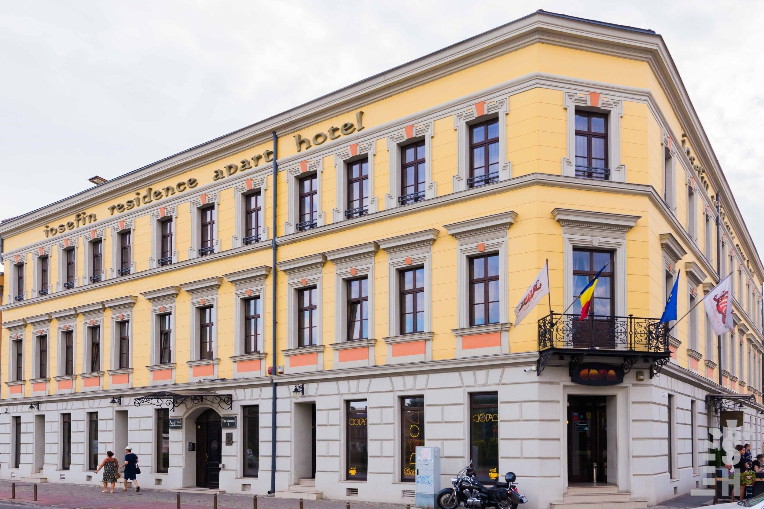
Figure 3: Original image

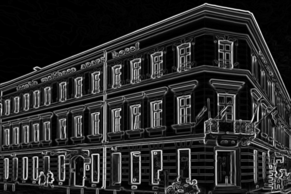
Figure 4: Proposed 3x3

Figure 5: Proposed A 5x5

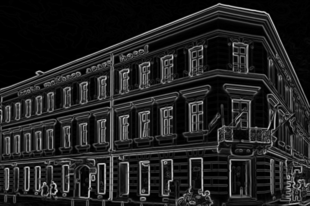
Figure 6: Proposed B 5x5

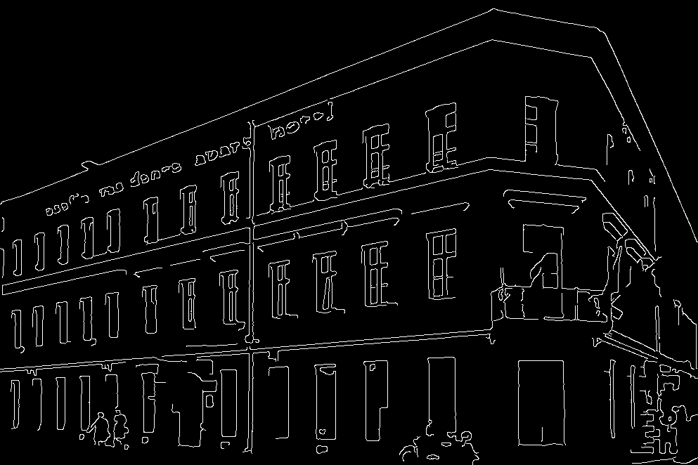
Figure 7: Canny Sobel 3x3

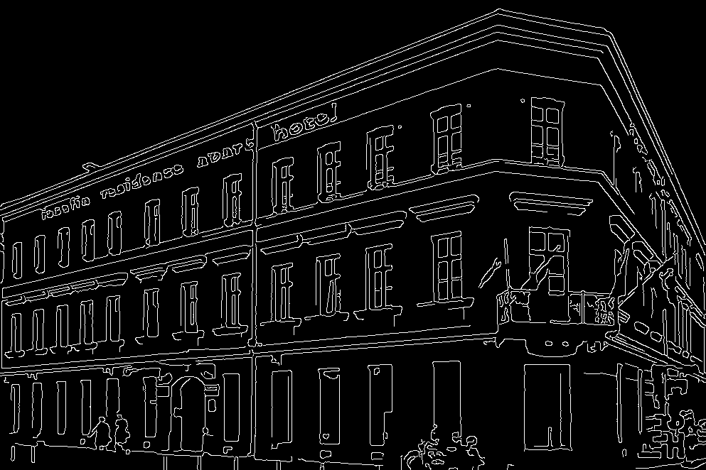
Figure 8: Canny Proposed A_B 3x3

Visually we can determine from Figures 5-8 that the 3x3 filters produce more concentrated edges than the 5x5 filters. But the 5x5 filters tend to lose a certain amount of detail on behalf of edges relevant for contour extraction.

As stated in section 3 to have a better idea about what edges have added value for a feature extraction based on them we would look over the results we got using the Canny algorithm [12, 18].

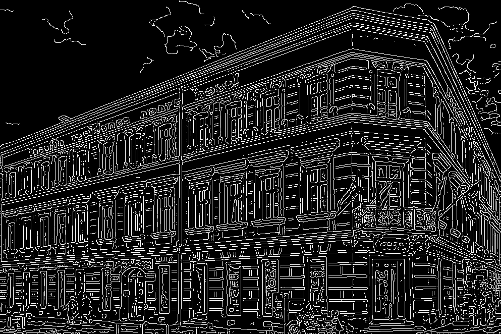
Figure 9: Canny Sobel 5x5

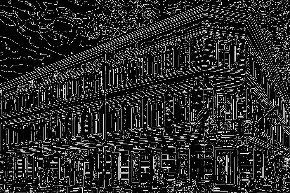
Figure 10: Canny Proposed A 5x5

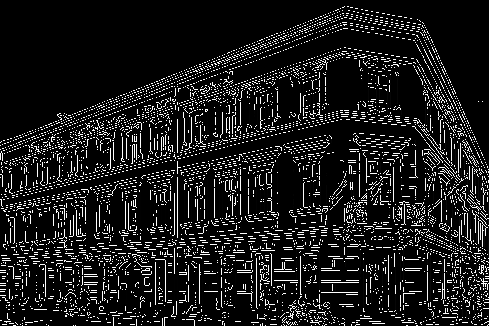
Figure 11: Canny Proposed B 5x5

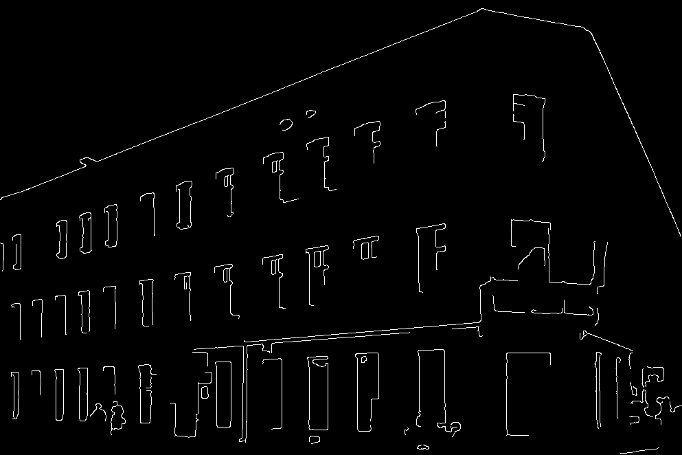
Figure 12: Canny Prewitt 3x3

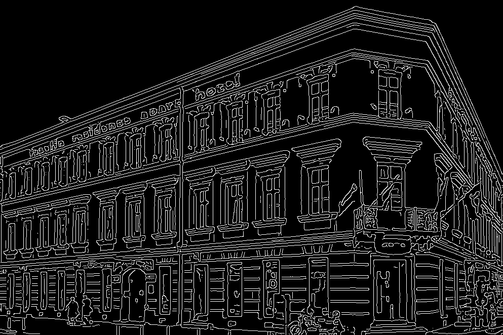
Figure 13: Canny Prewitt 5x5

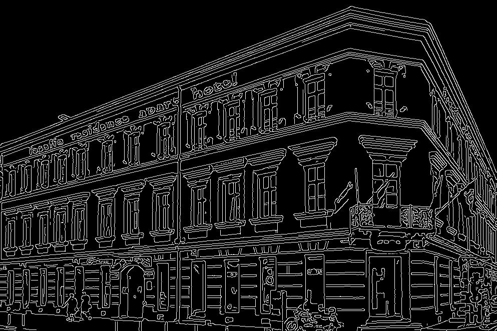
Figure 14: Canny Scharr 3x3

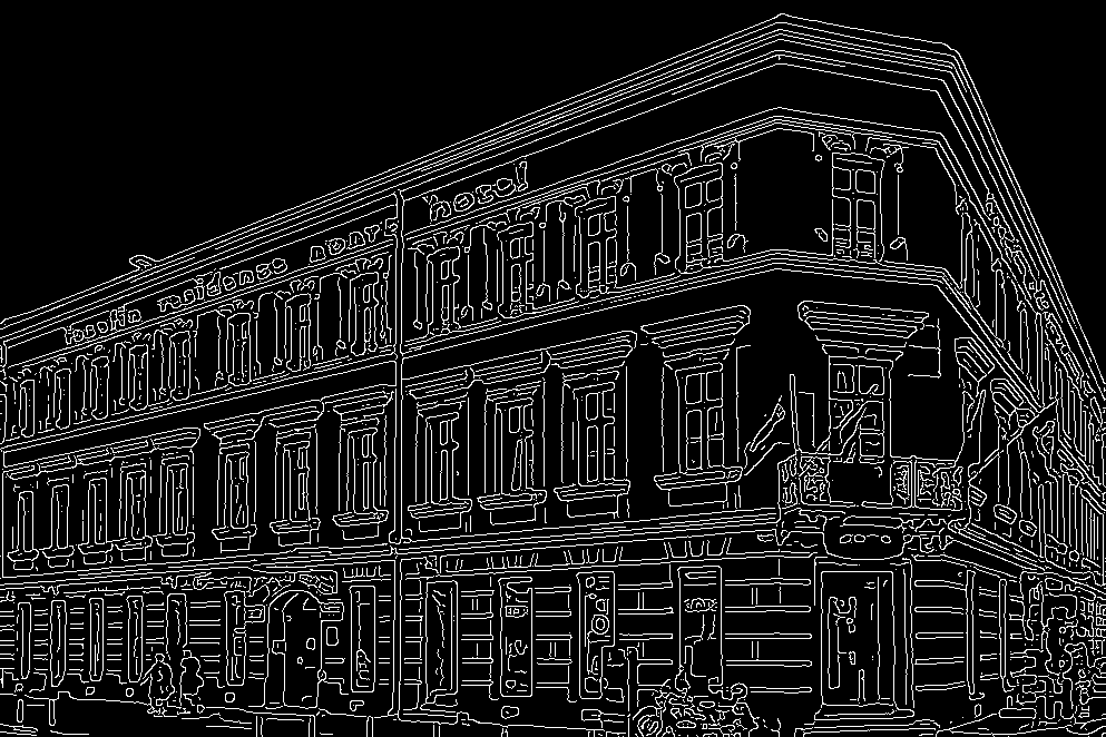
Figure 15: Canny Scharr 5x5

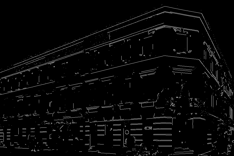
Figure 16: Canny Proposed A vs Sobel

Figure 17: Canny Sobel vs Proposed A

To obtain results that we can future use for contour detection or facade detection should be a balance between edges detected from the outer boundary of the building and facade details. The edges that do not belong to the buildings should be preferably discarded in this step. As we can see in Figures 8-17 the filters 3x3 obtain better results than the 5x5 ones.

Figure 11, 11 show a considerable amount of edges detected that we can consider noise and those edges will strongly affect any future use of those results.

Figure 11, 14, 14, 17 show good results in filtering out edges that are not in our interest but we can observe an extra amount of details on the facade detected that is not a benefit in future work.

The proposed filters and Sobel 3x3 [9] used in the Canny algorithm [12, 18], shown in Figure 8, 8, show good results in maintaining a balance between filtering out edges that we can consider noise and edges that we can future use for contour and edges that can be used for facade detection.

Naturally, we desired to better understand our results, so we took a dataset of 30 images that we used for Spotlight Heritage Timisoara project and compared the results obtained between Canny using Sobel 3x3 and Canny using our proposed filter.

The first result we saw was the fact that the number of edge pixels was always bigger, a fact that was observed from the images presented in this section. But we wanted to test our statement that the edge pixels we obtain form more and longer edges. To do that we used an eight-neighbor connectivity algorithm [21] and we can observe in Figure 19 and 19 the results.

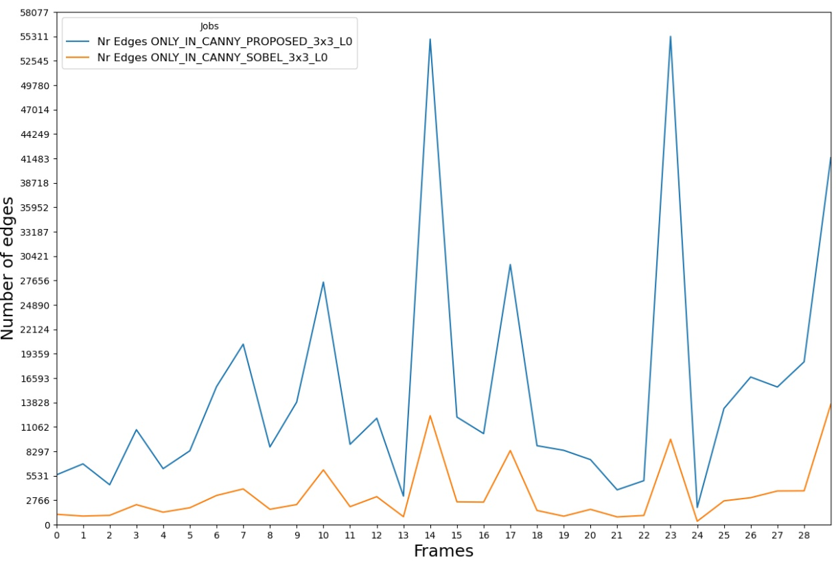
Figure 18: Number of edges found

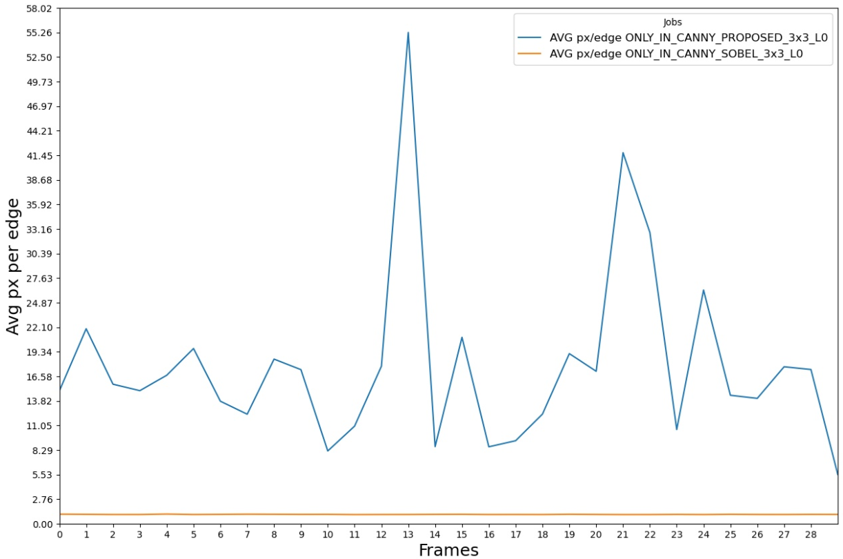
Figure 19: Average pixels per edge

In Figure 19 we observe that in every case our Canny using our proposed filter obtains more edge pixels that formed more edges than the Canny using Sobel filter. This fact alone does not prove that the edges found are useful but if we look on Figure 19 we can observe that those edges group in longer edges. We can clearly observe that the edges pixels found by the Sobel filter and not by our filter are sporadic pixels.

6 Conclusion and Future work

It is difficult to design a general edge detection algorithm which performs well in many contexts and captures the requirements of subsequent processing stages. With this research paper, we aimed to find a better fitted first derivative operator for building contour and facade edge detection.

We proposed two filters that have the same kernels for 3x3 but with different kernels for 5x5. As we can observe from Figure 17 our proposed filter managed to detect the same edges using the classical Sobel filter when used in the Canny algorithm.

As future work we plan to try the 3x3 filter operator, that obtains the best results, on a bigger data set of pictures with an official benchmarking tool for edge detection so we can assert statistically the improvements the proposed filter brings in this use case. At this point we analyzed the differences this filter brought to edge detection feature, as future work we would like to see the effect it has in contour detection algorithm, respective in facade detection algorithm.

This work will be valuable in improving the augmented reality mobile application of the Spotlight Heritage Timisoara project that the authors of this paper are involved in.

References

- [1] P. Milgram and F. Kishino, “A taxonomy of mixed reality visual displays,” IEICE TRANSACTIONS on Information and Systems, vol. 77, no. 12, pp. 1321–1329, 1994.
- [2] W. G. Wright, “Using virtual reality to augment perception, enhance sensorimotor adaptation, and change our minds,” Frontiers in systems neuroscience, vol. 8, p. 56, 2014.
- [3] S. Vert, B. Dragulescu, and R. Vasiu, “Lod4ar: Exploring linked open data with a mobile augmented reality web application.,” in International Semantic Web Conference (Posters & Demos), pp. 185–188, Citeseer, 2014.
- [4] S. Vert and R. Vasiu, “Relevant aspects for the integration of linked data in mobile augmented reality applications for tourism,” in International Conference on Information and Software Technologies, pp. 334–345, Springer, 2014.
- [5] S. Vert and R. Vasiu, “Augmented reality lenses for smart city data: the case of building permits,” in World Conference on Information Systems and Technologies, pp. 521–527, Springer, 2017.
- [6] S. Vert, D. Andone, and R. Vasiu, “Augmented and virtual reality for public space art,” in ITM Web of Conferences, vol. 29, p. 03006, EDP Sciences, 2019.
- [7] A. R. Elshehaby and L. G. E.-d. Taha, “A new expert system module for building detection in urban areas using spectral information and lidar data,” Applied Geomatics, vol. 1, no. 4, pp. 97–110, 2009.
- [8] “eLearning Center: Spotlight Heritage Timi\textcommabelowsoara.” Accessed: 2020/01/29.
- [9] I. Sobel and G. Feldman, “A 3x3 isotropic gradient operator for image processing,” a talk at the Stanford Artificial Project in, pp. 271–272, 1968.
- [10] J. M. Prewitt, “Object enhancement and extraction,” Picture processing and Psychopictorics, vol. 10, no. 1, pp. 15–19, 1970.
- [11] H. Scharr, Optimal operators in digital image processing. PhD thesis, 2000.
- [12] J. Canny, “A computational approach to edge detection,” IEEE Transactions on pattern analysis and machine intelligence, no. 6, pp. 679–698, 1986.
- [13] G. Takacs, M. El Choubassi, Y. Wu, and I. Kozintsev, “3d mobile augmented reality in urban scenes,” in 2011 ieee international conference on multimedia and expo, pp. 1–4, IEEE, 2011.
- [14] G. Reitmayr and T. W. Drummond, “Going out: robust model-based tracking for outdoor augmented reality,” in 2006 IEEE/ACM international symposium on mixed and augmented reality, pp. 109–118, IEEE, 2006.
- [15] J. Karlekar, S. Z. Zhou, W. Lu, Z. C. Loh, Y. Nakayama, and D. Hii, “Positioning, tracking and mapping for outdoor augmentation,” in 2010 ieee international symposium on mixed and augmented reality, pp. 175–184, IEEE, 2010.
- [16] S. Blanco-Pons, B. Carrión-Ruiz, M. Duong, J. Chartrand, S. Fai, and J. L. Lerma, “Augmented reality markerless multi-image outdoor tracking system for the historical buildings on parliament hill,” Sustainability, vol. 11, no. 16, p. 4268, 2019.
- [17] G. Levkine, “Prewitt, sobel and scharr gradient 5x5 convolution matrices,” Image Process. Articles, Second Draft, 2012.
- [18] M. Fang, G. Yue, and Q. Yu, “The study on an application of otsu method in canny operator,” in Proceedings. The 2009 International Symposium on Information Processing (ISIP 2009), p. 109, Citeseer, 2009.
- [19] A. S. Fotheringham and P. A. Rogerson, The SAGE handbook of spatial analysis. Sage, 2008.
- [20] R. M. Haralick and L. Watson, “A facet model for image data,” Computer Graphics and Image Processing, vol. 15, no. 2, pp. 113–129, 1981.
- [21] P. Bhattacharya and A. Rosenfeld, “a-convexity,” Pattern Recognition Letters, vol. 21, no. 10, pp. 955–957, 2000.