QLSD: Quantised Langevin Stochastic Dynamics for Bayesian Federated Learning

Abstract

The objective of Federated Learning (FL) is to perform statistical inference for data which are decentralised and stored locally on networked clients. FL raises many constraints which include privacy and data ownership, communication overhead, statistical heterogeneity, and partial client participation. In this paper, we address these problems in the framework of the Bayesian paradigm. To this end, we propose a novel federated Markov Chain Monte Carlo algorithm, referred to as Quantised Langevin Stochastic Dynamics which may be seen as an extension to the FL setting of Stochastic Gradient Langevin Dynamics, which handles the communication bottleneck using gradient compression. To improve performance, we then introduce variance reduction techniques, which lead to two improved versions coined QLSD^⋆ and QLSD⁺⁺. We give both non-asymptotic and asymptotic convergence guarantees for the proposed algorithms. We illustrate their performances using various Bayesian Federated Learning benchmarks.

1 INTRODUCTION

A paradigm shift has occurred with Federated Learning (FL) (McMahan et al., 2017; Kairouz et al., 2021). In FL, multiple entities (called clients) which own locally stored data collaborate in learning a “global” model which can then be “adapted” to each client. In the canonical FL, this task is coordinated by a central server. The initial focus of FL was on mobile and edge device applications, but recently there has been a surge of interest in applying the FL framework to other scenarios; in particular, those involving a small number of trusted clients (e.g. multiple organisations, enterprises, or other stakeholders).

FL has become one of the most active areas of artificial intelligence research over the past 5 years. FL differs significantly from the classical (distributed) ML setup (McMahan et al., 2017): the storage, computational, and communication capacities of each client vary amongst each other. This poses considerable challenges to successfully deal with many constraints raised by (i) partial client participation (e.g. in mobile applications, a client is not always active); (ii) communication bottleneck (clients are communication-constrained with limited bandwidth usage); (iii) model update synchronisation and merging.

Table 1: Overview of the main existing distributed/federated approximate Bayesian approaches. Column Comm. overhead gives the scheme employed to address the communication bottleneck. Column Heterogeneity means that the proposed approach tackles the impact of data heterogeneity on convergence while column Bounds highlights available non-asymptotic convergence guarantees.

Method	Comm. overhead	Heterogeneity	Partial participation	Bounds
Hasenclever et al. (2017)	local steps	✗	✗	✗
Nemeth and Sherlock (2018)	one-shot	✗	✗	✗
Bui et al. (2018)	local steps	✗	✓	✗
Jordan et al. (2019)	one-shot	✗	✗	✓
Corinzia et al. (2019)	local steps	✗	✓	✗
Kassab and Simeone (2020)	local steps	✗	✓	✗
El Mekkaoui et al. (2021)	local steps	✗	✗	✓
Plassier et al. (2021)	local steps	✗	✗	✓
Chen and Chao (2021)	local steps	✓	✓	✗
Liu and Simeone (2021a)	one-shot	✗	✗	✗
This work	compression	✓	✓	✓

Many methods derived from stochastic gradient descent techniques have been proposed in the literature to meet the specific FL constraints (McMahan et al., 2017; Alistarh et al., 2017; Horváth et al., 2019; Karimireddy et al., 2020; Li et al., 2020; Philippenko and Dieuleveut, 2020), see Wang et al. (2021) for a recent comprehensive overview. Whilst these approaches have successfully solved important issues associated to FL, they are unfortunately unable to capture and quantify epistemic predictive uncertainty which is essential in many applications such as autonomous driving or precision medicine (Hunter, 2016; Franchi et al., 2020). Indeed, these methods only provide a point estimate being a minimiser of a target empirical risk function. In contrast, the Bayesian paradigm (Robert, 2001) stands for a natural candidate to quantify uncertainty by providing a full description of the posterior distribution of the parameter of interest, and as such has become ubiquitous in the machine learning community (Andrieu et al., 2003; Hoffman et al., 2013; Izmailov et al., 2020, 2021).

In the last decade, many research efforts have been made to adapt serial workhorses of Bayesian computational methods such as variational inference, expectation-propagation, and Markov chain Monte Carlo (MCMC) algorithms to massively distributed architectures (Wang and Dunson, 2013; Ahn et al., 2014; Wang et al., 2015; Hasenclever et al., 2017; Bui et al., 2018; Jordan et al., 2019; Rendell et al., 2021; Vono et al., 2022). Since the main bottleneck in distributed computing is the communication overhead, these approaches mainly focus on deriving efficient algorithms specifically designed to meet such a constraint, requiring only periodic or few rounds of communication between a central server and clients; see Plassier et al. (2021, Section 4) for a recent overview. As highlighted in Table 1, most current Bayesian FL methods adapt these approaches and focus almost exclusively on Federated Averaging type updates (McMahan et al., 2017), performing multiple local steps on each client. This is in contrast with predictive FL algorithms (which are not estimating predictive uncertainty), for which a variety of schemes have been explored, e.g. via gradient compression or client subsampling (Wang et al., 2021, Section 3.1.2). Moreover, very few Bayesian FL works have attempted to address the challenges raised by partial device participation or the impact of statistical heterogeneity; see Liu and Simeone (2021b); Chen and Chao (2021). Convergence results in Bayesian FL lag far behind “canonical” FL.

In this paper, we attempt to fill this gap, by proposing novel MCMC methods that extend Stochastic Langevin Dynamics to the FL context. It is assumed that the clients’ data are independent and that the global posterior density is therefore the product of the non-identical local posterior densities of each client. To meet the specificity of Bayesian FL, each iteration of the proposed approaches only requires that a subset of active clients compute a stochastic gradient oracle for their associated negative log posterior density and send a lossy compression of these stochastic gradient oracles to the central server. The first scheme we derive, referred to as Quantised Langevin Stochastic Dynamics (QLSD), can interestingly be seen as the MCMC counterpart of the QSGD approach in FL (Alistarh et al., 2017), just as the Stochastic Gradient Langevin Dynamics (SGLD) (Welling and Teh, 2011) extends the Stochastic Gradient Descent (SGD). However, QLSD has the same drawbacks as SGLD: in particular, the invariant distribution of QLSD may deviate from the target distribution and become similar to the invariant measure of SGD when the number of observations is large (Brosse et al., 2018). We overcome this problem by deriving two variance-reduced versions QLSD^⋆ and QLSD⁺⁺ that both include control variates.

Contributions

(1) We propose a general MCMC algorithm called QLSD specifically designed for Bayesian inference under the FL paradigm and two variance-reduced alternatives, especially tackling heterogeneity, communication overhead and partial participation. (2) We provide a non-asymptotic convergence analysis of the proposed algorithms. The theoretical analysis highlights the impact of statistical heterogeneity measured by the discrepancy between local posterior distributions. (3) We propose efficient mechanisms to mitigate the impact of statistical heterogeneity on convergence, either by using biased stochastic gradients or by introducing a memory mechanism that extends Horváth et al. (2019) to the Bayesian setting. In particular, we find that variance reduction indeed allows the proposed MCMC algorithm to converge towards the desired target posterior distribution when the number of observations becomes large. (4) We illustrate the advantages of the proposed methods using several FL benchmarks. We show that the proposed methodology performs well compared to state-of-the-art Bayesian FL methods.

Notations and Conventions

The Euclidean norm on $\mathbb{R}^{d}$ is denoted by $\|\cdot\|$ and we set $\mathbb{N}^{*}=\mathbb{N}\setminus\{0\}$. For $n\in\mathbb{N}^{*}$, we refer to $\{1,\ldots,n\}$ with the notation $[n]$. For $N\in\mathbb{N}^{*}$, we use $\wp_{N}$ to denote the power set of $[N]$ and define $\wp_{N,n}=\{x\in\wp_{N}\,:\,\mathrm{card}(x)=n\}$ for any $n\in[N]$. We denote by $\mathrm{N}(m,\Sigma)$ the Gaussian distribution with mean vector $m$ and covariance matrix $\Sigma$. We define the sign function, for any $x\in\mathbb{R}$, as $\mathrm{sign}(x)=\mathbf{1}\{x\geq 0\}-\mathbf{1}\{x<0\}$. We define the Wasserstein distance of order $2$ for any probability measures $\mu,\nu$ on $\mathbb{R}^{d}$ with finite $2$-moment by $W_{2}(\mu,\nu)=(\inf_{\zeta\in\mathcal{T}(\mu,\nu)}\int_{\mathbb{R}^{d}\times\mathbb{R}^{d}}\|\theta-\theta^{\prime}\|^{2}\mathrm{d}\zeta(\theta,\theta^{\prime}))^{1/2}$, where $\mathcal{T}(\mu,\nu)$ is the set of transference plans of $\mu$ and $\nu$.

2 QUANTISED LANGEVIN STOCHASTIC DYNAMICS

In this section, we present the Bayesian FL framework and introduce the proposed methodology called QLSD along with two variance-reduced instances.

Problem Statement

We are interested in performing Bayesian inference on a parameter $\theta\in\mathbb{R}^{d}$ based on a training dataset $\mathrm{D}$. We assume that the posterior distribution admits a product-form density with respect to the $d$-dimensional Lebesgue measure, i.e.

$$\pi\left({\theta\mid\mathrm{D}}\right)=\mathrm{Z}_{\pi}^{-1}\,\textstyle\prod_{i=1}^{b}\mathrm{e}^{-U_{i}(\theta)}\,,$$ (1)

where $b\in\mathbb{N}^{*}$ and $\mathrm{Z}_{\pi}=\int_{\mathbb{R}^{d}}\prod_{i=1}^{b}\mathrm{e}^{-U_{i}(\theta)}\,\mathrm{d}\theta$ is a normalisation constant. This framework naturally encompasses the considered Bayesian FL problem. In this context, $\{\mathrm{e}^{-U_{i}}\}_{i\in[b]}$ stand for the unnormalised local posterior density functions associated to $b$ clients, where each client $i\in[b]$ is assumed to own a local dataset $\mathrm{D}_{i}$ such that $\mathrm{D}=\sqcup_{i=1}^{b}\mathrm{D}_{i}$. The dependency of $U_{i}$ on the local dataset $\mathrm{D}_{i}$ is omitted for brevity. A real-world illustration of the considered Bayesian problem is “multi-site fMRI classification” where each site (or client) owns a dataset coming from a local distribution because the methods of data generation and collection differ between sites. This results in different local likelihood functions, which combined with a local prior distribution, lead to heterogeneous local posteriors.

As in embarrassingly parallel MCMC approaches (Neiswanger et al., 2014), (1) implicitly assumes that the prior can be factorized across clients, which can always be done although the choice of this factorization is an open question. This product-form formulation can be alleviated by considering a global prior on $\theta$ and only calculating its gradient contribution on the central server during computations, see Algorithm 1.

A popular approach to sample from a target distribution with density $\pi$ defined in (1) is based on Langevin dynamics with stochastic gradient which, starting from an initial point $\theta_{0}$, defines a Markov chain $(\theta_{k})_{k\in\mathbb{N}}$ by recursion:

$$\theta_{k+1}=\theta_{k}-\gamma H_{k+1}({\textstyle{\theta_{k}}})+\sqrt{2\gamma}Z_{k+1}\,,\quad k\in\mathbb{N}\,,$$ (2)

where $\gamma\in\left(0,\bar{\gamma}\right]$, for some $\bar{\gamma}>0$, is a discretisation time step, $(Z_{k})_{k\in\mathbb{N}^{*}}$ is a sequence of i.i.d. standard Gaussian random variables and $(H_{k})_{k\in\mathbb{N}^{*}}$ stand for unbiased estimators of $\nabla U$ with $U=\sum_{i=1}^{b}U_{i}$ (Parisi, 1981; Grenander and Miller, 1994; Roberts and Tweedie, 1996). In a serial setting involving a single client which owns a dataset of size $N\in\mathbb{N}^{*}$, the potential $U$ writes $U=U_{1}=\sum_{j=1}^{N}U_{1,j}$ for some functions $U_{1,j}:\mathbb{R}^{d}\to\mathbb{R}$, and a popular instance of this framework is SGLD (Welling and Teh, 2011). This algorithm consists in the recursion (2) with the specific choice $H_{k+1}(\theta)=(N/n)\sum_{j\in\mathcal{S}_{k+1}}\nabla U_{1,j}(\theta)$, where $(\mathcal{S}_{k})_{k\in\mathbb{N}^{*}}$ is a sequence of i.i.d. uniform random subsets of $[N]$ of cardinal $n$.

In the FL framework, we assume that at each iteration $k$, the $i$-th client has access to an oracle $H_{k+1}^{(i)}$ based on its local negative log posterior density $U_{i}$, depending only on $\mathrm{D}_{i}$, so that $H_{k+1}=\sum_{i=1}^{b}H_{k+1}^{(i)}$ is a stochastic gradient oracle of $U$. Note that we do not assume that $H_{k+1}^{(i)}$ is an unbiased estimator of $\nabla U_{i}$, but only assume that $H_{k+1}$ is unbiased. This allows us to consider biased local stochastic gradient oracles with better convergence guarantees, see Section 3 for more details. A simple adaptation of SGLD to the FL framework under consideration is given by recursion:

$$\theta_{k+1}=\theta_{k}-\gamma\textstyle\sum_{i=1}^{b}H_{k+1}^{(i)}({\textstyle{\theta_{k}}})+\sqrt{2\gamma}Z_{k+1}\,,k\in\mathbb{N}\,.$$ (3)

If for any $i\in[b]$, every potential function $U_{i}$ also admits a finite-sum expression i.e. $U_{i}=\sum_{j=1}^{N_{i}}U_{i,j}$, similar to SGLD, we can for example use the local stochastic gradient oracles $H_{k+1}^{(i)}(\theta)=(N_{i}/n_{i})\sum_{j\in\mathcal{S}^{(i)}_{k+1}}\nabla U_{i,j}(\theta)$, where $(\mathcal{S}^{(i)}_{k+1})_{k\in\mathbb{N}^{*},\,i\in[b]}$ stand for i.i.d. uniform random subsets of $[N_{i}]$ of cardinal $n_{i}$. However, considering the MCMC algorithm associated with the recursion (3) is not adapted to the FL context. Indeed, this algorithm would assume that each client is reliable and suffers from the same issues as SGD in a risk-based minimisation context, especially a prohibitive communication overhead (Girgis et al., 2020).

Proposed Methodology

To address this problem, we propose to both account for the partial participation of clients and reduce the number of bits transmitted during the upload period by performing a lossy compression of a subset of $\{H_{k+1}^{(i)}\}_{i\in[b],k\in\mathbb{N}^{*}}$. This method has been used extensively in the “canonical” FL literature (Alistarh et al., 2017; Lin et al., 2018; Haddadpour et al., 2020; Sattler et al., 2020), but interestingly has never been considered in Bayesian FL; see Table 1.

To this end, we introduce a compression operator $\mathscr{C}:\mathbb{R}^{d}\to\mathbb{R}^{d}$ that is unbiased, i.e. for any $v\in\mathbb{R}^{d}$, $\mathbb{E}[\mathscr{C}(v)]=v$. In recent years, numerous compression operators have been proposed (Seide et al., 2014; Aji and Heafield, 2017; Stich et al., 2018). For example, the QSGD approach proposed in Alistarh et al. (2017) is based on stochastic quantisation.

QSGD considers for $\mathscr{C}$ a component-wise quantisation operator parameterised by a number of quantisation levels $s\geq 1$, which for each $j\in[d]$ and $v=(v_{1},\ldots,v_{d})\in\mathbb{R}^{d}$ are given by

$$\mathscr{C}^{(s,j)}(v)=\frac{\left\|{v}\right\|\mathrm{sign}(v_{j})}{s}\left({l_{j}+\mathbf{1}\left\{{\xi_{j}\leq\frac{s|v_{j}|}{\left\|{v}\right\|}-l_{j}}\right\}}\right),$$ (4)

where $l_{j}=\left\lfloor s|v_{j}|/\left\|{v}\right\|\right\rfloor$ and $\{\xi_{j}\}_{j\in[d]}$ is a sequence of i.i.d. uniform random variables on $[0,1]$. In this particular case, we will denote the quantisation of $v$ via (4) by $\mathscr{C}^{(s)}(v)=\{\mathscr{C}^{(s,j)}(v)\}_{j\in[d]}$.

The proposed general methodology, called Quantised Langevin Stochastic Dynamics (QLSD) stands for a compressed and FL version of the specific instance of SGLD defined in (3). More precisely, QLSD is an MCMC algorithm associated with the Markov chain $(\theta_{k})_{k\in\mathbb{N}}$ starting from $\theta_{0}$ and defined for $k\in\mathbb{N}$ as

$$\theta_{k+1}=\ \theta_{k}-\gamma\frac{b}{|\mathcal{A}_{k+1}|}\sum_{i\in\mathcal{A}_{k+1}}\mathscr{C}_{k+1}\left[{H_{k+1}^{(i)}({\textstyle{\theta_{k}}})}\right]$$

$$+\sqrt{2\gamma}Z_{k+1}\,,$$

where $({\textstyle{\mathcal{A}_{k}}})_{k\in\mathbb{N}^{*}}$ denotes the subset of active (i.e. available) clients at iteration $k$, possibly random. Note that we indexed $\mathscr{C}$ by $k+1$ to emphasize that this compression operator is a stochastic operator and hence varies across iterations, see e.g. (4). The derivation of QLSD in the considered Bayesian FL context is described in details in Algorithm 1. A generalisation of QLSD taking into account heterogeneous communication constraints between clients by considering different compression operators $\{\mathscr{C}^{(i)}\}_{i\in[b]}$ is available in the Supplementary Material, see e.g. Section S1. In the particular case of the finite-sum setting where each client owns a dataset of size $N_{i}$, i.e. for the choice $H^{(i)}_{k+1}(\theta)=(N_{i}/n_{i})\sum_{j\in\mathcal{S}_{k+1}^{(i)}}\nabla U_{i,j}(\theta)$ for $\theta\in\mathbb{R}^{d}$, $\mathcal{S}_{k+1}^{(i)}\in\wp_{N_{i},n_{i}}$, we denote the corresponding instance of QLSD as $\texttt{QLSD}^{\#}$.

In this paper, we have decided to focus only on a non-adjusted sampling algorithm (QLSD) since the derivations of non-asymptotic results are already consequent, see the Supplementary Material. In addition, up to authors’ knowledge, a general consensus on the choice between Metropolis-adjusted algorithms and their unadjusted counterparts has not been achieved yet.

Algorithm 1 Quantised Langevin Stochastic Dynamics (QLSD)

Input: nb. iterations $K$, compression operators $\{\mathscr{C}_{k+1}\}_{k\in\mathbb{N}}$, stochastic gradients $\{H_{k+1}^{(i)}\}_{i\in[b],k\in\mathbb{N}}$, step-size $\gamma\in(0,\bar{\gamma}]$ and initial point $\theta_{0}$.

for $k=0$ to $K-1$ do

     for $i\in\mathcal{A}_{k+1}$ // On active clients $\mathcal{A}_{k+1}$ do

         Compute $\textsl{g}_{i,k+1}=\mathscr{C}_{k+1}\left[{H_{k+1}^{(i)}({\textstyle{\theta_{k}}})}\right]$.

         Send $\textsl{g}_{i,k+1}$ to the central server.

     end for

      // On the central server

     Compute $\textsl{g}_{k+1}=\frac{b}{|\mathcal{A}_{k+1}|}\sum_{i\in\mathcal{A}_{k+1}}\textsl{g}_{i,k+1}$.

     Draw $Z_{k+1}\sim\mathrm{N}(0_{d},\mathrm{I}_{d})$

     Compute $\theta_{k+1}=\theta_{k}-\gamma\textsl{g}_{k+1}+\sqrt{2\gamma}Z_{k+1}$.

     Send $\theta_{k+1}$ to the $b$ clients.

end for

Output: samples $\{\theta_{k}\}_{k=0}^{K}$.

Variance-Reduced Alternatives

Consider the finite-sum setting i.e. for any $i\in[b]$, $U_{i}=\sum_{j=1}^{N_{i}}U_{i,j}$ where $N_{i}$ is the size of the local dataset $\mathrm{D}_{i}$. As highlighted in Section 1, SGLD-based approaches, including Algorithm 1, involve an invariant distribution that may deviate from the target posterior distribution when $\min_{i\in b}N_{i}$ goes to infinity, as stochastic gradients with large variance are used (Brosse et al., 2018; Baker et al., 2019). We deal with this problem by proposing two variance-reduced alternatives of $\texttt{QLSD}^{\#}$  that use control variates. The simplest variance-reduced approach, referred to as QLSD^⋆ (see Algorithm S1) and discussed in more details in the Supplementary Material (see Section S2), considers a fixed-point approach that uses a minimiser $\theta^{\star}$ of the potential $U$ (Brosse et al., 2018; Baker et al., 2019) defined as

$$\theta^{\star}\in\operatornamewithlimits{\arg\min}_{\theta\in\mathbb{R}^{d}}\sum_{i=1}^{b}U_{i}(\theta)\,.$$ (5)

In this scenario, the stochastic gradient oracles write for each $i\in[b]$, $k\in\mathbb{N}^{*}$, $\theta\in\mathbb{R}^{d}$ and $\mathcal{S}_{k+1}^{(i)}\in\wp_{N_{i},n_{i}}$, $H_{k+1}^{(i)}(\theta)=(N_{i}/n_{i})\sum_{j\in\mathcal{S}_{k+1}^{(i)}}[\nabla U_{i,j}(\theta)-\nabla U_{i,j}(\theta^{\star})]$. Although $\mathbb{E}[H_{k+1}]=\nabla U$, note that for each $i\in[b]$, $\mathbb{E}[H_{k+1}^{(i)}]\neq\nabla U_{i}$ so $H_{k+1}^{(i)}$ is not an unbiased estimate of $U_{i}$. We show in Section 3 that introducing this bias improves the convergence properties of $\texttt{QLSD}^{\#}$ with respect to the discrepancy between local posterior distributions. Since estimating $\theta^{\star}$ in a FL context might impose an additional computational burden on the sampling procedure, we propose another variance-reduced alternative referred to as QLSD⁺⁺ (see Algorithm 2). This method builds on the Stochastic Variance Reduced Gradient (SVRG): it uses control variates $(\zeta_{k})_{k\in\mathbb{N}}$ that are updated every $l\in\mathbb{N}^{*}$ iterations (Johnson and Zhang, 2013) and at each iteration $k\in\mathbb{N}$ and for any client $i\in[b]$, the stochastic gradient oracle $H_{k+1}^{(i)}$ defined by $H_{k+1}^{(i)}(\theta)=(N_{i}/n_{i})\sum_{j\in\mathcal{S}_{k+1}^{(i)}}[\nabla U_{i,j}(\theta)-\nabla U_{i,j}(\zeta_{k})]+\nabla U_{i}(\zeta_{k})$. To reduce the impact of local posterior discrepancy on convergence, we take inspiration from the “canonical” FL literature and consider a memory term $(\eta^{(i)}_{k})_{k\in\mathbb{N}}$ on each client $i\in[b]$ (Horváth et al., 2019; Dieuleveut et al., 2020). At each iteration $k$, instead of directly compressing $H_{k+1}^{(i)}$, we compress the difference $H_{k+1}^{(i)}-\eta^{(i)}_{k}$, store it in $\textsl{g}_{i,k+1}$, and then compute the global stochastic gradient $\textsl{g}_{k+1}=\frac{b}{|\mathcal{A}_{k+1}|}\sum_{i\in\mathcal{A}_{k+1}}\textsl{g}_{i,k+1}+\sum_{i=1}^{b}\eta^{(i)}_{k}$. The memory term $(\eta^{(i)}_{k})_{k\in\mathbb{N}}$ is then updated on each client $i\in[b]$, by the recursion $\eta^{(i)}_{k+1}=\eta^{(i)}_{k}+\alpha\mathbf{1}_{\mathcal{A}_{k+1}}(i)\textsl{g}_{i,k+1}$. The benefits of using this memory mechanism will be assessed theoretically in Section 3 and illustrated numerically in Section S5.2 in the Supplementary Material.

Algorithm 2 Variance-reduced Quantised Langevin Stochastic Dynamics (QLSD⁺⁺)

Input: minibatch sizes $\{n_{i}\}_{i\in[b]}$, number of iterations $K$, compression operators $\{\mathscr{C}_{k+1}\}_{k\in\mathbb{N}^{*}}$, step-size $\gamma\in(0,\bar{\gamma}]$ with $\bar{\gamma}>0$, initial point $\theta_{0}$ and $\alpha\in(0,\bar{\alpha}]$ with $\bar{\alpha}>0$.

// Memory mechanism initialisation

Initialise $\{\eta^{(1)}_{0},\ldots,\eta^{(b)}_{0}\}$ and $\eta_{0}=\sum_{i=1}^{b}\eta^{(i)}_{0}$.

for $k=0$ to $K-1$ do

      // Update of the control variates

     if $k\equiv 0$ ($\mathrm{mod}\ l$) then

         Set $\zeta_{k}=\theta_{k}$.

     else

         Set $\zeta_{k}=\zeta_{k-1}$

     end if

     for $i\in\mathcal{A}_{k+1}$ // On active clients do

         Draw $\mathcal{S}_{k+1}^{(i)}\sim\mathrm{Uniform}\left({\wp_{N_{i},n_{i}}}\right)$.

         Set $H_{k+1}^{(i)}(\theta_{k})=(N_{i}/n_{i})\sum_{j\in\mathcal{S}_{k+1}^{(i)}}[\nabla U_{i,j}(\theta_{k})-\nabla U_{i,j}(\zeta_{k})]+\nabla U_{i}(\zeta_{k})$.

         Compute $\textsl{g}_{i,k+1}=\mathscr{C}_{k+1}\left({H_{k+1}^{(i)}(\theta_{k})-\eta^{(i)}_{k}}\right)$.

         Send $\textsl{g}_{i,k+1}$ to the central server.

         Set $\eta^{(i)}_{k+1}=\eta^{(i)}_{k}+\alpha\textsl{g}_{i,k+1}$.

     end for

      // On the central server

     Compute $\textsl{g}_{k+1}=\eta_{k}+\frac{b}{|\mathcal{A}_{k+1}|}\sum_{i\in\mathcal{A}_{k+1}}\textsl{g}_{i,k+1}$.

     Set $\eta_{k+1}=\eta_{k}+\alpha\sum_{i\in\mathcal{A}_{k+1}}^{b}\textsl{g}_{i,k+1}$.

     Draw $Z_{k+1}\sim\mathrm{N}(0_{d},\mathrm{I}_{d})$.

     Compute $\theta_{k+1}=\theta_{k}-\gamma\textsl{g}_{k+1}+\sqrt{2\gamma}Z_{k+1}$.

     Send $\theta_{k+1}$ to the $b$ clients.

end for

Output: samples $\{\theta_{k}\}_{k=0}^{K}$.

3 THEORETICAL ANALYSIS

This section provides a detailed theoretical analysis of the proposed methodology. In particular, we will show the impact of using stochastic gradients, partial participation and compression by deriving quantitative convergence bounds for QLSD, which is detailed in Algorithm 1. We then derive non-asymptotic convergence bounds for QLSD^⋆ and QLSD⁺⁺, and explicitly show that these variance-reduced algorithms indeed succeed in reducing both the variance caused by stochastic gradients and the effects of local posterior discrepancy in the bounds we obtain for $\texttt{QLSD}^{\#}$. We consider the following assumptions on the potential $U$.

H 1.

For any $i\in[b]$, $U_{i}$ is continuously differentiable. In addition, suppose that the following hold.

1. $U$ is $\mathtt{m}$-strongly convex, i.e. for any $\theta_{1},\theta_{2}\in\mathbb{R}^{d}$, $\langle\nabla U(\theta_{1})-\nabla U(\theta_{2}),\theta_{1}-\theta_{2}\rangle\geq\mathtt{m}\left\|{\theta_{1}-\theta_{2}}\right\|^{2}$.

2. $U$ is $\mathtt{L}$-Lipschitz, i.e. for any $\theta_{1},\theta_{2}\in\mathbb{R}^{d}$, $\left\|{\nabla U\left({\theta_{1}}\right)-\nabla U\left({\theta_{2}}\right)}\right\|\leq\mathtt{L}\left\|{\theta_{1}-\theta_{2}}\right\|$.

Note that 1-(i) implies that $U$ admits a unique minimiser denoted by $\theta^{\star}\in\mathbb{R}^{d}$.

The compression operators $\{\mathscr{C}_{k+1}\}_{k\in\mathbb{N}}$ are assumed to satisfy the following assumption.

H 2.

The compression operators $\{\mathscr{C}_{k+1}\}_{k\in\mathbb{N}}$ are independent and satisfy the following conditions.

1. For any $k\in\mathbb{N}^{*}$, $v\in\mathbb{R}^{d}$, $\mathbb{E}[\mathscr{C}_{k}({\textstyle{v}})]=v$.

2. There exists $\omega\geq 1$, such that for any $k\in\mathbb{N}^{*}$, $v\in\mathbb{R}^{d}$, $\mathbb{E}[\left\|{\mathscr{C}_{k}({\textstyle{v}})-v}\right\|^{2}]\leq\omega\left\|{v}\right\|^{2}$.

As an example, the assumption on the variance of the compression operator detailed in 2-(ii) is verified for the quantisation operator $\mathscr{C}^{(s)}$ defined in (4) with $\omega=\min(d/s^{2},\sqrt{d}/s)$ (Alistarh et al., 2017, Lemma 3.1).

Non-Asymptotic Analysis for Algorithm 1

We consider the following assumptions on the stochastic gradient oracles used in QLSD.

H 3.

The random fields $\{{\textstyle{H_{k+1}^{(i)}:\mathbb{R}^{d}\to\mathbb{R}^{d}}}\}_{i\in[b],k\in\mathbb{N}}$ are independent and satisfy the following conditions.

1. For any $\theta\in\mathbb{R}^{d}$ and $k\in\mathbb{N}$, $\sum_{i=1}^{b}\mathbb{E}[H_{k+1}^{(i)}({\textstyle{\theta}})]=\nabla U\left({\theta}\right)$.

2. There exist $\{\mathtt{M}_{i}>0\}_{i\in[b]}$, such that for any $i\in[b]$, $k\in\mathbb{N}$, $\theta_{1},\theta_{2}\in\mathbb{R}^{d}$, $\mathbb{E}\left[{\left\|{H_{k+1}^{(i)}({\textstyle{\theta_{1}}})-H_{k+1}^{(i)}({\textstyle{\theta_{2}}})}\right\|^{2}}\right]\leq\mathtt{M}_{i}\left\langle{\theta_{1}-\theta_{2}},{\nabla U_{i}\left({\theta_{1}}\right)-\nabla U_{i}\left({\theta_{2}}\right)}\right\rangle.$

3. There exist $\sigma_{\star},\mathtt{B}^{\star}\in\mathbb{R}_{+}$ such that for any $\theta\in\mathbb{R}^{d}$, $k\in\mathbb{N}$, we have $\mathbb{E}\left[{\left\|{H_{k+1}^{(i)}({\textstyle{\theta^{\star}}})}\right\|}\right]^{2}\leq\mathtt{B}^{\star}/b$, and $\mathbb{E}\left[{\left\|{\textstyle\sum_{i=1}^{b}H_{k+1}^{(i)}(\theta^{\star})}\right\|^{2}}\right]\leq\sigma_{\star}^{2}$, where $\theta^{\star}$ is defined in (5).

We can notice that 3-(ii) implies that $\nabla U_{i}$ is $\mathtt{M}_{i}$-Lipschitz continuous since by the Cauchy-Schwarz inequality, for any $i\in[b]$ and any $\theta_{1},\theta_{2}\in\mathbb{R}^{d}$, $\left\|{\nabla U_{i}\left({\theta_{1}}\right)-\nabla U_{i}\left({\theta_{2}}\right)}\right\|^{2}\leq\mathtt{M}_{i}\left\langle{\theta_{1}-\theta_{2}},{\nabla U_{i}\left({\theta_{1}}\right)-\nabla U_{i}\left({\theta_{2}}\right)}\right\rangle$. Conversely, in the finite-sum setting, 3-(ii) is satisfied by $\texttt{QLSD}^{\#}$ with $\mathtt{M}_{i}=N_{i}\bar{\mathtt{M}}$ if for any $i\in[b]$ and $j\in[N_{i}]$, $U_{i,j}$ is convex and $\nabla U_{i,j}$ is $\bar{\mathtt{M}}$-Lipschitz continuous, for $\bar{\mathtt{M}}\geq 0$ by Nesterov (2003, Theorem 2.1.5).

Table 2: Order of the asymptotic biases $\{B_{\bar{\gamma}},B_{\mathbin{\mathchoice{\ooalign{$\displaystyle\vbox{\hbox{\scalebox{0.77778}{$\displaystyle\bigcirc$}}}$\cr$\displaystyle\star$\cr}}{\ooalign{$\textstyle\vbox{\hbox{\scalebox{0.77778}{$\textstyle\bigcirc$}}}$\cr$\textstyle\star$\cr}}{\ooalign{$\scriptstyle\vbox{\hbox{\scalebox{0.77778}{$\scriptstyle\bigcirc$}}}$\cr$\scriptstyle\star$\cr}}{\ooalign{$\scriptscriptstyle\vbox{\hbox{\scalebox{0.77778}{$\scriptscriptstyle\bigcirc$}}}$\cr$\scriptscriptstyle\star$\cr}}},\bar{\gamma}},B_{\oplus,\bar{\gamma}}\}$, associated to the three proposed MCMC algorithms, in squared 2-Wasserstein distance for two types of asymptotic. Red dependencies prevent from (quick) convergence while green dependencies ensure convergence of associated MCMC algorithms. $\theta^{\star}$ is defined in (5).

Algo.	Bias		Dependencies of the asymptotic bias when $\bar{\gamma}\downarrow 0$				Dependencies of the asymptotic bias as $N_{i}\rightarrow\infty$
		$d$	$H_{k+1}^{(i)}$	$\mathtt{B}^{\star}$	partial particip.	$\omega$
QLSD	$B_{\bar{\gamma}}$	$d$	$\sigma^{2}_{\star}$	${\color[rgb]{1,0,0}\mathtt{B}^{\star}}$	$(1-p)/p$	$\omega$	${\color[rgb]{1,0,0}\operatorname{\mathrm{O}}(N_{i})}$
$\texttt{QLSD}^{\#}$	$B_{\bar{\gamma}}$	$d$	$N_{i}^{2}$	${\color[rgb]{1,0,0}\sum_{i=1}^{b}\left\|{\nabla U_{i}(\theta^{\star})}\right\|^{2}}$	$(1-p)/p$	$\omega$	${\color[rgb]{1,0,0}\operatorname{\mathrm{O}}(N_{i})}$
QLSD⋆	$B_{\mathbin{\mathchoice{\ooalign{$\displaystyle\vbox{\hbox{\scalebox{0.77778}{$\displaystyle\bigcirc$}}}$\cr$\displaystyle\star$\cr}}{\ooalign{$\textstyle\vbox{\hbox{\scalebox{0.77778}{$\textstyle\bigcirc$}}}$\cr$\textstyle\star$\cr}}{\ooalign{$\scriptstyle\vbox{\hbox{\scalebox{0.77778}{$\scriptstyle\bigcirc$}}}$\cr$\scriptstyle\star$\cr}}{\ooalign{$\scriptscriptstyle\vbox{\hbox{\scalebox{0.77778}{$\scriptscriptstyle\bigcirc$}}}$\cr$\scriptscriptstyle\star$\cr}}},\bar{\gamma}}$	$d$	$N_{i}$	-	$(1-p)/p$	$\omega$	${\color[rgb]{0,0.4,0}d\operatorname{\mathrm{O}}\left({1}\right)}$
QLSD++	$B_{\oplus,\bar{\gamma}}$	$d$	$N_{i}$	-	$(1-p)/p$	$\omega$	${\color[rgb]{0,0.4,0}d\operatorname{\mathrm{O}}\left({1}\right)}$

In addition, it is worth mentioning that the first inequality in 3-(iii) is also required for our derivation in the deterministic case where $H_{k+1}^{(i)}=\nabla U_{i}$ due to the compression operator. In this particular case, $\mathtt{B}^{\star}$ stands for an upper-bound on $\sum_{i=1}^{b}\left\|{\nabla U_{i}(\theta^{\star})}\right\|^{2}$ and corresponds to some discrepancy between local posterior density functions meaning that $\nabla U_{i}\neq\nabla U$ for $i\in[b]$. This phenomenon, referred to as data heterogeneity in the risk-based literature (Horváth et al., 2019; Karimireddy et al., 2020), is ubiquitous in the FL context.

Finally, we assume for simplicity that clients’ partial participation is realised by each client having probability $p\in(0,1]$ of being active in each communication round.

H 4.

For any $k\in\mathbb{N}^{*}$, $\mathcal{A}_{k}=\{i\in[b]\,:\,B_{i,k}=1\}$ where $\{B_{i,k}\,:\,i\in[b]\,,\,k\in\mathbb{N}^{*}\}$ is a family of i.i.d. Bernouilli random variables with success probability $p\in\left(0,1\right]$.

A generalisation of this scheme considering different probabilities $p_{i}$ per client can be found in the Supplementary Material, see e.g. Section S1.1. Under the above assumptions and by denoting $Q_{\gamma}$ the Markov kernel associated to Algorithm 1, the following convergence result holds.

Theorem 1.

Assume 1, 2, 3 and 4. Then, there exists $\bar{\gamma}_{\infty}$ such that for $\bar{\gamma}<\bar{\gamma}_{\infty}$, there exist $A_{\bar{\gamma}},B_{\bar{\gamma}}>0$ (explicitly given in Section S1 in the Supplementary Material) satisfying for any probability measure $\mu\in\mathcal{P}_{2}\left({\mathbb{R}^{d}}\right)$, any step size $\gamma\in\left(0,\bar{\gamma}\right]$ and $k\in\mathbb{N}$,

$$W_{2}^{2}\left({\mu Q_{\gamma}^{k},\pi}\right)\leq(1-\gamma\mathtt{m}/2)^{k}\cdot W_{2}^{2}\left({\mu,\pi}\right)+\gamma B_{\bar{\gamma}}$$

$$+\gamma^{2}A_{\bar{\gamma}}(1-\mathtt{m}\gamma/2)^{k-1}k\cdot\int_{\mathbb{R}^{d}}\|\theta-\theta^{\star}\|^{2}\mu(\mathrm{d}\theta)\,,$$

where $\theta^{\star}$ is defined in (5).

Similar to ULA (Dalalyan, 2017; Durmus and Moulines, 2019) and SGLD (Dalalyan and Karagulyan, 2019; Durmus et al., 2019), the upper bound given in Theorem 1 includes a contracting term that depends on the initialisation and a bias term $\gamma B_{\bar{\gamma}}$ that does not vanish with $k\rightarrow\infty$ due to the use of a fixed step size $\gamma$. In the asymptotic scenario, i.e. $\bar{\gamma}\downarrow 0$, Table 1 gives the dependencies of $B_{\bar{\gamma}}$ for QLSD  and its particular instance $\texttt{QLSD}^{\#}$, in terms of key quantities associated with the setting we consider. Similar to SGLD, we can observe that the use of stochastic gradients entails a bias term of order $\sigma^{2}_{\star}\operatorname{\mathrm{O}}(\gamma)$. On the other hand, the use of partial participation and compression compared to SGLD introduces an additional bias of order $(\omega/p)(\mathtt{m}\mathtt{B}^{\star}+\mathtt{L}\mathtt{M}d)\operatorname{\mathrm{O}}(\gamma)$, which grows with in particular $\mathtt{B}^{\star}$, corresponding to the impact of the local posterior discrepancy on convergence.

Non-Asymptotic Analysis for Variance-Reduced Alternatives

We assume in the sequel that the potential functions $\{U_{i}\}_{i\in[b]}$ admit the finite-sum decomposition $U_{i}=\sum_{j=1}^{N_{i}}U_{i,j}$ for each $i\in[b]$ and consider the following assumptions.

H 5.

For any $i\in[b],j\in[N_{i}]$, $U_{i,j}$ is continuously differentiable and the following holds.

1. There exists $\mathtt{M}_{i}>0$ such that, for any $\theta_{1},\theta_{2}\in\mathbb{R}^{d}$, $\left\|{\nabla U_{i}(\theta_{2})-\nabla U_{i}(\theta_{1})}\right\|^{2}\leq\mathtt{M}\left\langle{\theta_{2}-\theta_{1}},{\nabla U_{i}(\theta_{2})-\nabla U_{i}(\theta_{1})}\right\rangle$.

2. There exists $\bar{\mathtt{M}}\geq 0$ such that, for any $\theta_{1},\theta_{2}\in\mathbb{R}^{d}$, $\left\|{\nabla U_{i,j}({\textstyle{\theta_{2}}})-\nabla U_{i,j}({\textstyle{\theta_{1}}})}\right\|^{2}\leq\bar{\mathtt{M}}\left\langle{\nabla U_{i,j}({\textstyle{\theta_{2}}})-\nabla U_{i,j}({\textstyle{\theta_{1}}})},{\theta_{2}-\theta_{1}}\right\rangle$.

As mentioned earlier, 5 is satisfied if for every $i\in[b]$ and $j\in[N_{i}]$, $U_{i,j}$ is convex and $\nabla U_{i,j}$ is $\bar{\mathtt{M}}$-Lipschitz continuous. Under these additional conditions, the following non-asymptotic convergence results hold for the two reduced-variance MCMC algorithms described in Section 2. Denote by $Q_{\mathbin{\mathchoice{\ooalign{$\displaystyle\vbox{\hbox{\scalebox{0.77778}{$\displaystyle\bigcirc$}}}$\cr$\displaystyle\star$\cr}}{\ooalign{$\textstyle\vbox{\hbox{\scalebox{0.77778}{$\textstyle\bigcirc$}}}$\cr$\textstyle\star$\cr}}{\ooalign{$\scriptstyle\vbox{\hbox{\scalebox{0.77778}{$\scriptstyle\bigcirc$}}}$\cr$\scriptstyle\star$\cr}}{\ooalign{$\scriptscriptstyle\vbox{\hbox{\scalebox{0.77778}{$\scriptscriptstyle\bigcirc$}}}$\cr$\scriptscriptstyle\star$\cr}}},\gamma}$ the Markov kernel associated to $\texttt{QLSD}^{\star}$  with a step size $\gamma\in\left(0,\bar{\gamma}\right]$.

Theorem 2.

Assume 1, 2, 4 and 5. Then, there exists $\bar{\gamma}_{\mathbin{\mathchoice{\ooalign{$\displaystyle\vbox{\hbox{\scalebox{0.77778}{$\displaystyle\bigcirc$}}}$\cr$\displaystyle\star$\cr}}{\ooalign{$\textstyle\vbox{\hbox{\scalebox{0.77778}{$\textstyle\bigcirc$}}}$\cr$\textstyle\star$\cr}}{\ooalign{$\scriptstyle\vbox{\hbox{\scalebox{0.77778}{$\scriptstyle\bigcirc$}}}$\cr$\scriptstyle\star$\cr}}{\ooalign{$\scriptscriptstyle\vbox{\hbox{\scalebox{0.77778}{$\scriptscriptstyle\bigcirc$}}}$\cr$\scriptscriptstyle\star$\cr}}},\infty}$ such that for $\bar{\gamma}<\bar{\gamma}_{\mathbin{\mathchoice{\ooalign{$\displaystyle\vbox{\hbox{\scalebox{0.77778}{$\displaystyle\bigcirc$}}}$\cr$\displaystyle\star$\cr}}{\ooalign{$\textstyle\vbox{\hbox{\scalebox{0.77778}{$\textstyle\bigcirc$}}}$\cr$\textstyle\star$\cr}}{\ooalign{$\scriptstyle\vbox{\hbox{\scalebox{0.77778}{$\scriptstyle\bigcirc$}}}$\cr$\scriptstyle\star$\cr}}{\ooalign{$\scriptscriptstyle\vbox{\hbox{\scalebox{0.77778}{$\scriptscriptstyle\bigcirc$}}}$\cr$\scriptscriptstyle\star$\cr}}},\infty}$, there exist $A_{\mathbin{\mathchoice{\ooalign{$\displaystyle\vbox{\hbox{\scalebox{0.77778}{$\displaystyle\bigcirc$}}}$\cr$\displaystyle\star$\cr}}{\ooalign{$\textstyle\vbox{\hbox{\scalebox{0.77778}{$\textstyle\bigcirc$}}}$\cr$\textstyle\star$\cr}}{\ooalign{$\scriptstyle\vbox{\hbox{\scalebox{0.77778}{$\scriptstyle\bigcirc$}}}$\cr$\scriptstyle\star$\cr}}{\ooalign{$\scriptscriptstyle\vbox{\hbox{\scalebox{0.77778}{$\scriptscriptstyle\bigcirc$}}}$\cr$\scriptscriptstyle\star$\cr}}},\bar{\gamma}},B_{\mathbin{\mathchoice{\ooalign{$\displaystyle\vbox{\hbox{\scalebox{0.77778}{$\displaystyle\bigcirc$}}}$\cr$\displaystyle\star$\cr}}{\ooalign{$\textstyle\vbox{\hbox{\scalebox{0.77778}{$\textstyle\bigcirc$}}}$\cr$\textstyle\star$\cr}}{\ooalign{$\scriptstyle\vbox{\hbox{\scalebox{0.77778}{$\scriptstyle\bigcirc$}}}$\cr$\scriptstyle\star$\cr}}{\ooalign{$\scriptscriptstyle\vbox{\hbox{\scalebox{0.77778}{$\scriptscriptstyle\bigcirc$}}}$\cr$\scriptscriptstyle\star$\cr}}},\bar{\gamma}}>0$ (explicitly given in Section S2 in the Supplementary Material) satisfying for any probability measure $\mu\in\mathcal{P}_{2}\left({\mathbb{R}^{d}}\right)$, any step size $\gamma\in\left(0,\bar{\gamma}\right]$ and $k\in\mathbb{N}$,

$$W_{2}^{2}\left({\mu Q_{\mathbin{\mathchoice{\ooalign{$\displaystyle\vbox{\hbox{\scalebox{0.77778}{$\displaystyle\bigcirc$}}}$\cr$\displaystyle\star$\cr}}{\ooalign{$\textstyle\vbox{\hbox{\scalebox{0.77778}{$\textstyle\bigcirc$}}}$\cr$\textstyle\star$\cr}}{\ooalign{$\scriptstyle\vbox{\hbox{\scalebox{0.77778}{$\scriptstyle\bigcirc$}}}$\cr$\scriptstyle\star$\cr}}{\ooalign{$\scriptscriptstyle\vbox{\hbox{\scalebox{0.77778}{$\scriptscriptstyle\bigcirc$}}}$\cr$\scriptscriptstyle\star$\cr}}},\gamma}^{k},\pi}\right)\leq(1-\gamma\mathtt{m}/2)^{k}\cdot W_{2}^{2}\left({\mu,\pi}\right)+\gamma B_{\mathbin{\mathchoice{\ooalign{$\displaystyle\vbox{\hbox{\scalebox{0.77778}{$\displaystyle\bigcirc$}}}$\cr$\displaystyle\star$\cr}}{\ooalign{$\textstyle\vbox{\hbox{\scalebox{0.77778}{$\textstyle\bigcirc$}}}$\cr$\textstyle\star$\cr}}{\ooalign{$\scriptstyle\vbox{\hbox{\scalebox{0.77778}{$\scriptstyle\bigcirc$}}}$\cr$\scriptstyle\star$\cr}}{\ooalign{$\scriptscriptstyle\vbox{\hbox{\scalebox{0.77778}{$\scriptscriptstyle\bigcirc$}}}$\cr$\scriptscriptstyle\star$\cr}}},\bar{\gamma}}$$

$$+\gamma^{2}A_{\mathbin{\mathchoice{\ooalign{$\displaystyle\vbox{\hbox{\scalebox{0.77778}{$\displaystyle\bigcirc$}}}$\cr$\displaystyle\star$\cr}}{\ooalign{$\textstyle\vbox{\hbox{\scalebox{0.77778}{$\textstyle\bigcirc$}}}$\cr$\textstyle\star$\cr}}{\ooalign{$\scriptstyle\vbox{\hbox{\scalebox{0.77778}{$\scriptstyle\bigcirc$}}}$\cr$\scriptstyle\star$\cr}}{\ooalign{$\scriptscriptstyle\vbox{\hbox{\scalebox{0.77778}{$\scriptscriptstyle\bigcirc$}}}$\cr$\scriptscriptstyle\star$\cr}}},\bar{\gamma}}(1-\mathtt{m}\gamma/2)^{k-1}k\cdot\int_{\mathbb{R}^{d}}\|\theta-\theta^{\star}\|^{2}\mu(\mathrm{d}\theta)\,,$$

where $\theta^{\star}$ is defined in (5).

Compared to QLSD and $\texttt{QLSD}^{\star}$, QLSD⁺⁺ only defines an inhomogeneous Markov chain, see Section S3.3 in the Supplementary Material for more details. For a step-size $\gamma\in\left(0,\bar{\gamma}\right]$ and an iteration $k\in\mathbb{N}$, we denote by $\mu Q_{\oplus,\gamma}^{(k)}$ the distribution of $\theta_{k}$ defined by $\texttt{QLSD}^{++}$ starting from $\theta_{0}$ with distribution $\mu$.

Theorem 3.

Assume 1, 2, 4 and 5, and let $l\in\mathbb{N}^{*}$ and $\alpha\in(0,1/(\omega+1)]$. Then, there exists $\bar{\gamma}_{\oplus,\infty}$ such that for $\bar{\gamma}<\bar{\gamma}_{\oplus,\infty}$, there exist $A_{\oplus,\bar{\gamma}},B_{\oplus,\bar{\gamma}},C_{\oplus,\bar{\gamma}}>0$ (explicitly given in Section S3 in the Supplementary Material and independent of $\alpha$) satisfying for any probability measure $\mu\in\mathcal{P}_{2}\left({\mathbb{R}^{d}}\right)$, any step size $\gamma\in\left(0,\bar{\gamma}\right]$ and $k\in\mathbb{N}$,

$$W_{2}^{2}({\textstyle{\mu Q_{\mathbin{\mathchoice{\ooalign{$\displaystyle\vbox{\hbox{\scalebox{0.77778}{$\displaystyle\bigcirc$}}}$\cr$\displaystyle+$\cr}}{\ooalign{$\textstyle\vbox{\hbox{\scalebox{0.77778}{$\textstyle\bigcirc$}}}$\cr$\textstyle+$\cr}}{\ooalign{$\scriptstyle\vbox{\hbox{\scalebox{0.77778}{$\scriptstyle\bigcirc$}}}$\cr$\scriptstyle+$\cr}}{\ooalign{$\scriptscriptstyle\vbox{\hbox{\scalebox{0.77778}{$\scriptscriptstyle\bigcirc$}}}$\cr$\scriptscriptstyle+$\cr}}},\gamma}^{(k)},\pi}})\leq(1-\gamma\mathtt{m}/2)^{k}\cdot W_{2}^{2}\left({\mu,\pi}\right)+\gamma B_{\oplus,\bar{\gamma}}$$

$$+\gamma^{2}A_{\oplus,\bar{\gamma}}(1-\gamma\mathtt{m}/2)^{\left\lfloor k/l\right\rfloor}\cdot\int_{\mathbb{R}^{d}}\|\theta-\theta^{\star}\|^{2}\mu(\mathrm{d}\theta)$$

$$+\gamma C_{\oplus,\bar{\gamma}}[(1-\alpha)^{k}\wedge(1-\gamma\mathtt{m}/2)^{\left\lfloor k/l\right\rfloor}]\sum_{i=1}^{b}\left\|{\nabla U_{i}(\theta^{\star})}\right\|^{2},$$

where $\theta^{\star}$ is defined in (5).

Table 2 provides the dependencies of the asymptotic bias terms $B_{\mathbin{\mathchoice{\ooalign{$\displaystyle\vbox{\hbox{\scalebox{0.77778}{$\displaystyle\bigcirc$}}}$\cr$\displaystyle\star$\cr}}{\ooalign{$\textstyle\vbox{\hbox{\scalebox{0.77778}{$\textstyle\bigcirc$}}}$\cr$\textstyle\star$\cr}}{\ooalign{$\scriptstyle\vbox{\hbox{\scalebox{0.77778}{$\scriptstyle\bigcirc$}}}$\cr$\scriptstyle\star$\cr}}{\ooalign{$\scriptscriptstyle\vbox{\hbox{\scalebox{0.77778}{$\scriptscriptstyle\bigcirc$}}}$\cr$\scriptscriptstyle\star$\cr}}},\bar{\gamma}},B_{\oplus,\bar{\gamma}}$ as $\bar{\gamma}\downarrow 0$ with respect to key quantities associated to the problem we consider. For comparison, we do the same regarding the specific instance of Algorithm 1, QLSD^#. Remarkably, thanks to biased local stochastic gradients for QLSD^⋆ and the memory mechanism for QLSD⁺⁺, we can notice that their associated asymptotic biases do not depend on local posterior discrepancy in contrast to QLSD^#. This is in line with non-asymptotic convergence results in risk-based FL which also show that the impact of data heterogeneity can be alleviated using such a memory mechanism (Philippenko and Dieuleveut, 2020). The impact of stochastic gradients is discussed in further details in the next paragraph.

Consistency Analysis in the Big Data Regime

In Brosse et al. (2018), it was shown that ULA and SGLD define homogeneous Markov chains, each of which admits a unique stationary distribution. However, while the invariant distribution of ULA gets closer to $\pi$ as $N_{i}$ increases, conversely the invariant measure of SGLD never approaches $\pi$ and is in fact very similar to the invariant measure of SGD. Moreover, the non-compressed counterpart of QLSD^⋆ has been shown not to suffer from this problem, and it has been theoretically proven to be a viable alternative to ULA in the Big Data environment. Since QLSD  is a generalisation of SGLD, the conclusions of Brosse et al. (2018) hold. On the other hand, we show that the reduced-variance alternatives to QLSD that we introduced provide more accurate estimates of $\pi$ as $N_{i}$ increases, see the last column in Table 2. Detailed calculations are deferred to Section S4 in the Supplementary Material.

4 NUMERICAL EXPERIMENTS

This section illustrates our methodology with three numerical experiments that include both synthetic and real datasets. For all experiments, we consider the finite-sum setting and use the stochastic quantisation operator $\mathscr{C}^{(s)}$ for $s\geq 1$ defined in (4) to perform the compression step. In this case 2-(ii) is verified with $\omega=\min(d/s^{2},\sqrt{d}/s)$. Further experimental results are given in Section S5 in the Supplementary Material.

Figure 1: Toy Gaussian example. (top) 2D projection of the heterogeneous synthetic dataset where each color refers to a client and each dot is an observation $y_{i,j}$. (bottom) Estimation performances of the considered Bayesian FL algorithms.

Toy Gaussian Example

This first experiment aims at illustrating the general behavior of Algorithm 1 with respect to the use of stochastic gradients and compression scheme. To this purpose, we set $b=20$ and $d=50$ and consider a Gaussian posterior distribution with density defined in (1) where, for any $i\in[b]$ and $\theta\in\mathbb{R}^{d}$, $U_{i}(\theta)=\sum_{j=1}^{N_{i}}\|\theta-y_{i,j}\|^{2}/2$, $\{y_{i,j}\}_{i\in[b],j\in[N_{i}]}$ being a set of synthetic independent but not identically distributed observations across clients and $N_{i}\in[10,200]$, see Figure 1 (top row). Note that in this specific case, $\theta^{\star}$ admits a closed form expression. For all the algorithms, we choose the (optimised) step-size $\gamma=4.9\times 10^{-4}$ and choose a minibatch size $n_{i}=\left\lfloor N_{i}/10\right\rfloor$. Instances of $\texttt{QLSD}^{\#}$ and $\texttt{QLSD}^{\star}$ using $s=2^{p}$ are referred to as p-bits instances of these MCMC algorithms. We compare these algorithms with the non-compressed counterpart of $\texttt{QLSD}^{\star}$ referred to as LSD^⋆, see Algorithm S2. Figure 1 shows the behavior of the mean squarred error (MSE) associated to the test function $f:\theta\mapsto\left\|{\theta}\right\|$, computed using 30 independent runs of each algorithm, with respect to the number of bits transmitted. We can notice that $\texttt{QLSD}^{\star}$ always outperforms $\texttt{QLSD}^{\#}$and that decreasing the value of $\omega$ does not significantly reduce the bias associated to $\texttt{QLSD}^{\star}$. This illustrates the impact of the variance of the stochastic gradients and supports our theoretical analysis summarised in Table 2. On the other hand, QLSD^⋆ with $s=2^{16}$ achieves a similar MSE as LSD^⋆ while requiring roughly 2.5 times less number of bits.

Bayesian Logistic Regression

In this experiment, we compare the proposed methodology based on gradient compression with two existing FedAvg-type MCMC algorithms. Since $\theta^{\star}$ defined in (5) is not easily available, we implement QLSD⁺⁺ detailed in Algorithm 2. We adopt a zero-mean Gaussian prior with covariance matrix $2\cdot 10^{-2}\mathrm{I}_{d}$ and use the FEMNIST dataset (Caldas et al., 2018). We set $b=50$, $l=100$, $\alpha=1/(\omega+1)$ and $\gamma=10^{-5}$. We launch QLSD⁺⁺ for $s\in\{2^{4},2^{8},2^{16}\}$ and compare its performances with DG-SGLD (Plassier et al., 2021) and FSGLD (El Mekkaoui et al., 2021) which use multiple local steps to address the communication bottleneck. We are interested in performing uncertainty quantification by estimating highest posterior density (HPD) regions. For any $\alpha\in(0,1)$, we define $\mathcal{C}_{\alpha}=\{\theta\in\mathbb{R}^{d};-\log\pi(\theta|\mathrm{D})\leq\eta_{\alpha}\}$ where $\eta_{\alpha}\in\mathbb{R}$ is chosen such that $\int_{\mathcal{C}_{\alpha}}\pi(\theta|\mathrm{D})\mathrm{d}\theta=1-\alpha$. We compute the relative HPD error based on the scalar summary $\eta_{\alpha}$, i.e. $|\eta_{\alpha}-\eta_{\alpha}^{\texttt{LSD}}|/\eta_{\alpha}^{\texttt{LSD}}$ where $\eta_{\alpha}^{\texttt{LSD}}$ has been estimated using the non-compressed counterpart of QLSD⁺⁺, referred to as LSD⁺⁺ and standing for a serial variance-reduced SGLD, see Algorithm S3. Table 3 gives this relative HPD error for $\alpha=0.01$ and provides the relative efficiency of QLSD⁺⁺ and competitors corresponding to the savings in terms of transmitted bits per iteration. One can notice that the proposed approach provides similar results as its non-compressed counterpart while being 3 to 7 times more efficient. In addition, we show that QLSD⁺⁺ provides similar performances as DG-SGLD and FSGLD which highlight that gradient compression and periodic communication are competing approaches.

Table 3: Bayesian Logistic Regression.

Algorithm	99% HPD error	Rel. efficiency
FSGLD	5.4e-3	6.2
DG-SGLD	5.2e-3	6.4
QLSD++ 4 bits	6.1e-3	7.6
QLSD++ 8 bits	4.3e-3	6.7
QLSD++ 16 bits	6.9e-4	3.1

Table 4: Performances of Bayesian FL algorithms on the considered Bayesian neural networks problem.

Method	HMC	SGLD	QLSD++	QLSD++ PP	FedBe-Dirichlet	FedBe-Gauss.	DG-SGLD	FSGLD
Accuracy	89.6	88.8	88.1	86.6	90.7	90.2	92.2	87.5
Agreement	0.94	0.91	0.90	0.90	0.90	0.89	0.91	0.91
TV	0.07	0.11	0.12	0.12	0.16	0.16	0.13	0.13

Bayesian Neural Networks

In our third experiment, we go beyond the scope of our theoretical analysis by performing posterior inference in Bayesian neural networks. We use the ResNet-20 model (He et al., 2016), choose a zero-mean Gaussian prior distribution with variance $1/5$ and consider the classification problem associated with the CIFAR-10 dataset (Krizhevsky et al., 2009). We run QLSD⁺⁺ with $s=2$, $l=20$, $\alpha=1/(\omega+1)$, and with either $p=1$ (full participation) or $p=0.25$ (partial participation). We compare the proposed methodology with a long-run Hamiltonian Monte Carlo (HMC) considered as a “ground truth” (Izmailov et al., 2021) and SGLD. For completeness, we also implement four other distributed/federated approximate sampling approaches, namely two instances of FedBe (Chen and Chao, 2021), DG-SGLD and FSGLD. Following Wilson et al. (2021), we compare the aforementioned algorithms through three metrics: classification accuracy on the test dataset using the minimum mean-square estimator, agreement between the top-1 prediction given by each algorithm and the one given by HMC and total variation between approximate and “true” (associated with HMC) predictive distributions. More details about algorithms’ hyperparameters and considered metrics are given in Section S5.3 in the Supplementary Material. The results we obtain are gathered in Table 4. In terms of agreement and total variation, QLSD⁺⁺ (even with partial participation) gives similar results as SGLD and competes favorably with other existing federated approaches. Figure 2 complements this empirical analysis by showing calibration curves of posterior predictive distributions.

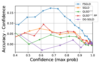
Figure 2: Bayesian Neural Networks.

5 CONCLUSION

In this paper, we presented a general methodology based on Langevin stochastic dynamics for Bayesian FL. In particular, we addressed the challenges associated with this new ML paradigm by assuming that a subset of clients sends compressed versions of its local stochastic gradient oracles to the central server. Moreover, the proposed method was found to have favorable convergence properties, as evidenced by numerical illustrations. In particular, it compares favorably to FedAvg-type Bayesian FL algorithms. A limitation of this work is that the proposed method does not target the initial posterior distribution due to the use of a fixed discretisation time step. Therefore, this work paves the way for more advanced Bayesian FL approaches based, for example, on Metropolis-Hastings schemes to remove asymptotic biases. In addition, although the data ownership issue is implicitly tackled by the FL paradigm by not sharing data, stronger privacy guarantees can be ensured, typically by combining differential privacy, secure multi-party computation and homomorphic encryption methods. Proposing a differentially private version of our methodology is a possible extension of our work, that is left for further work. This work has no direct societal impact.

Acknowledgements

The authors acknowledge support of the Lagrange Mathematics and Computing Research Center.

 

Supplementary Material:
QLSD: Quantised Langevin Stochastic Dynamics for Bayesian Federated Learning

 

Notations and conventions.

We denote by $\mathcal{B}(\mathbb{R}^{d})$ the Borel $\sigma$-field of $\mathbb{R}^{d}$, $\mathbb{M}(\mathbb{R}^{d})$ the set of all Borel measurable functions $f$ on $\mathbb{R}^{d}$ and $\left\|{\cdot}\right\|$ the Euclidean norm on $\mathbb{R}^{d}$. For $\mu$ a probability measure on $(\mathbb{R}^{d},\mathcal{B}(\mathbb{R}^{d}))$ and $f\in\mathbb{M}(\mathbb{R}^{d})$ a $\mu$-integrable function, denote by $\mu(f)$ the integral of $f$ with respect to (w.r.t.) $\mu$. Let $\mu$ and $\nu$ be two sigma-finite measures on $(\mathbb{R}^{d},\mathcal{B}(\mathbb{R}^{d}))$. Denote by $\mu\ll\nu$ if $\mu$ is absolutely continuous w.r.t. $\nu$ and $\mathrm{d}\mu/\mathrm{d}\nu$ the associated density. We say that $\zeta$ is a transference plan of $\mu$ and $\nu$ if it is a probability measure on $(\mathbb{R}^{d}\times\mathbb{R}^{d},\mathcal{B}(\mathbb{R}^{d}\times\mathbb{R}^{d}))$ such that for all measurable set $\mathsf{A}$ of $\mathbb{R}^{d}$, $\zeta(\mathsf{A}\times\mathbb{R}^{d})=\mu(\mathsf{A})$ and $\zeta(\mathbb{R}^{d}\times\mathsf{A})=\nu(\mathsf{A})$. We denote by $\mathcal{T}(\mu,\nu)$ the set of transference plans of $\mu$ and $\nu$. In addition, we say that a couple of $\mathbb{R}^{d}$-random variables $(X,Y)$ is a coupling of $\mu$ and $\nu$ if there exists $\zeta\in\mathcal{T}(\mu,\nu)$ such that $(X,Y)$ are distributed according to $\zeta$. We denote by $\mathcal{P}_{2}(\mathbb{R}^{d})$ the set of probability measures with finite $2$-moment: for all $\mu\in\mathcal{P}_{2}(\mathbb{R}^{d}),\int_{\mathbb{R}^{d}}\|x\|^{2}\mathrm{d}\mu(x)<\infty$. We define the squared Wasserstein distance of order $2$ associated with $\|\cdot\|$ for any probability measures $\mu,\nu\in\mathcal{P}_{2}(\mathbb{R}^{d})$ by

$$W_{2}^{2}(\mu,\nu)=\inf_{\zeta\in\mathcal{T}(\mu,\nu)}\int_{\mathbb{R}^{d}\times\mathbb{R}^{d}}\|x-y\|^{2}\mathrm{d}\zeta(x,y)\,.$$

By Villani (2008, Theorem 4.1), for all $\mu$, $\nu$ probability measures on $\mathbb{R}^{d}$, there exists a transference plan $\zeta^{\star}\in\mathcal{T}(\mu,\nu)$ such that for any coupling $(X,Y)$ distributed according to $\zeta^{\star}$, $W_{2}(\mu,\nu)=\mathbb{E}[\|x-y\|^{2}]^{1/2}$. This kind of transference plan (respectively coupling) will be called an optimal transference plan (respectively optimal coupling) associated with $W_{2}$. By Villani (2008, Theorem 6.16), $\mathcal{P}_{2}(\mathbb{R}^{d})$ equipped with the Wasserstein distance $W_{2}$ is a complete separable metric space. For the sake of simplicity, with little abuse, we shall use the same notations for a probability distribution and its associated probability density function. For $n\geq 1$, we refer to the set of integers between $1$ and $n$ with the notation $[n]$ and $\wp_{n}$ the power set of $[n]$. The $d$-multidimensional Gaussian probability distribution with mean $\mu\in\mathbb{R}^{d}$ and covariance matrix $\Sigma\in\mathbb{R}^{d\times d}$ is denoted by $\mathrm{N}(\mu,\Sigma)$.

Appendix S1 PROOF OF Theorem 1

This section aims at proving Theorem 1 in the main paper.

S1.1 Generalised quantised Langevin stochastic dynamics

We show that QLSD defined in Algorithm 1 in the main paper can be cast into a more general framework that we refer to as generalised quantised Langevin stochastic dynamics. Then, the guarantees for QLSD will be a simple consequence of the ones that we will establish for generalised QLSD. For ease of reading, we recall first the setting and the assumptions that we consider all along the paper. Recall that the dataset $\mathrm{D}$ is assumed to be partitioned into $b$ shards $\{\mathrm{D}_{i}\}_{i=1}^{b}$ such that $\sqcup_{i=1}^{b}\mathrm{D}_{i}=\mathrm{D}$ and the posterior distribution of interest is assumed to admit a density with respect to the $d$-dimensional Lebesgue measure which factorises across clients, i.e. for any $\theta\in\mathbb{R}^{d}$,

$$\pi(\theta)=\exp\left\{{-U(\theta)}\right\}/\int_{\mathbb{R}^{d}}\mathrm{e}^{-U(\theta)}\,\mathrm{d}\theta\,, U(\theta)=\sum_{i=1}^{b}U_{i}(\theta)\,.$$

We consider the following assumptions on the potential $U$.

H S1.

For any $i\in[b]$, $U_{i}$ is continuously differentiable. In addition, suppose that the following conditions hold.

1. $U$ is $\mathtt{m}$-strongly convex, i.e. for any $\theta_{1},\theta_{2}\in\mathbb{R}^{d}$,

   $$U(\theta_{1})\geq U(\theta_{2})+\left\langle{\theta_{1}-\theta_{2}},{\nabla U(\theta_{2})}\right\rangle+\mathtt{m}\left\|{\theta_{1}-\theta_{2}}\right\|^{2}/2\,.$$

2. $U$ is $\mathtt{L}$-Lipschitz, i.e. for any $\theta_{1},\theta_{2}\in\mathbb{R}^{d}$,

   $$\left\|{\nabla U(\theta_{1})-\nabla U(\theta_{2})}\right\|\leq\mathtt{L}\left\|{\theta_{1}-\theta_{2}}\right\|\,.$$

Note that S1-(i) implies that $U$ admits a unique minimiser denoted by $\theta^{\star}\in\mathbb{R}^{d}$. Moreover, for any $(\theta_{1},\theta_{1})\in\mathbb{R}^{d}$, S1-(i)-(ii) combined with Nesterov (2003, Equation 2.1.24) shows that

$$\left\langle{\nabla U(\theta_{2})-\nabla U(\theta_{1})},{\theta_{2}-\theta_{1}}\right\rangle\geq\frac{\mathtt{m}\mathtt{L}}{\mathtt{m}+\mathtt{L}}\left\|{\theta_{2}-\theta_{1}}\right\|^{2}+\frac{1}{\mathtt{m}+\mathtt{L}}\left\|{\nabla U(\theta_{2})-\nabla U(\theta_{1})}\right\|^{2}\,.$$ (S1)

We consider the following assumptions on the family $\{{\textstyle{H_{i}:\mathbb{R}^{d}\times\mathsf{X}_{1}\to\mathbb{R}^{d}}}\}_{i\in[b]}$ and $\mathscr{C}$.

H S2.

There exists a probability measure $\nu_{2}$ on a measurable space $(\mathsf{X}_{2},\mathcal{X}_{2})$ and a family of measurable functions $\{\mathscr{C}_{i}:\mathbb{R}^{d}\times\mathsf{X}_{2}\to\mathbb{R}^{d}\}_{i\in[b]}$ such that the following conditions hold.

1. For any $\theta\in\mathbb{R}^{d}$ and any $i\in[b]$, $\int_{\mathsf{X}_{2}}\mathscr{C}_{i}(\theta,x^{(2)})\,\nu_{2}(\mathrm{d}x^{(2)})=\theta$.

2. There exist $\{\omega_{i}\in\mathbb{R}_{+}\}_{i\in[b]}$, such that for any $\theta\in\mathbb{R}^{d}$ and any $i\in[b]$,

   $$\int_{\mathsf{X}_{2}}\left\|{\mathscr{C}_{i}(\theta,x^{(2)})-\theta}\right\|^{2}\,\nu_{2}(\mathrm{d}x^{(2)})\leq\omega_{i}\left\|{\theta}\right\|^{2}\,.$$

H S3.

There exist a family of probability measures $\{\nu_{1}^{(i)}\}_{i\in[b]}$ defined on measurable spaces $\{(\mathsf{X}_{1}^{(i)},\mathcal{X}_{1}^{(i)})\}_{i\in[b]}$ and a family of measurable functions $\{{\textstyle{H_{i}:\mathbb{R}^{d}\times\mathsf{X}_{1}^{(i)}\to\mathbb{R}^{d}}}\}_{i\in[b]}$ such that the following conditions hold.

1. For any $\theta\in\mathbb{R}^{d}$,

   $$\sum_{i=1}^{b}\int_{\mathsf{X}_{1}^{(i)}}H_{i}(\theta,x^{(1,i)})\nu_{1}^{(i)}(\mathrm{d}x^{(1,i)})=\nabla U(\theta)\,.$$

2. There exist $\{\mathtt{M}_{i}>0\}_{i\in[b]}$, such that for any $i\in[b]$, $\theta_{1},\theta_{2}\in\mathbb{R}^{d}$,

   $$\int_{\mathsf{X}_{1}^{(i)}}\left\|{H_{i}(\theta_{2},x^{(1,i)})-H_{i}(\theta_{1},x^{(1,i)})}\right\|^{2}\nu_{1}^{(i)}(\mathrm{d}x^{(1,i)})\leq\mathtt{M}_{i}\left\langle{\theta_{2}-\theta_{1}},{\nabla U_{i}(\theta_{2})-\nabla U_{i}(\theta_{1})}\right\rangle\,.$$

3. There exists $\sigma_{\star},\mathtt{B}^{\star}\in\mathbb{R}_{+}$ such that for any $i\in[b]$, $\theta\in\mathbb{R}^{d}$, we have

   $$\int_{\mathsf{X}_{1}^{(i)}}\left\|{H_{i}(\theta^{\star},x^{(1)})}\right\|^{2}\nu_{1}^{(i)}(\mathrm{d}x^{(1)})\leq\mathtt{B}^{\star}/b\,, \int_{\mathsf{X}_{1}^{(1)}\times\cdots\times\mathsf{X}_{1}^{(b)}}\left\|{\sum_{i=1}^{b}H_{i}(\theta^{\star},x^{(1,i)})}\right\|^{2}\otimes_{i=1}^{b}\nu_{1}^{(i)}(\mathrm{d}x^{(1,i)})\leq\sigma_{\star}^{2}\,.$$ (S2)

We can notice that S3-(ii) implies that $\nabla U_{i}$ is $\mathtt{M}_{i}$-Lipschitz continuous since by the Cauchy Schwarz inequality, for any $i\in[b]$ and any $\theta_{1},\theta_{2}\in\mathbb{R}^{d}$,

$$\left\|{\nabla U_{i}(\theta_{1})-\nabla U_{i}(\theta_{2})}\right\|^{2}\leq\mathtt{M}_{i}\left\langle{\theta_{1}-\theta_{2}},{\nabla U_{i}(\theta_{1})-\nabla U_{i}(\theta_{2})}\right\rangle\,.$$

In addition, it is worth mentioning that the first inequality in (S2) is also required for our derivation in the deterministic case where $H_{i}=\nabla U_{i}$ for any $i\in[b]$ due to the compression step. For $k\geq 1$, consider $(X_{k}^{(1,1)},\ldots,X_{k}^{(1,b)})_{k\in\mathbb{N}}$ and $(X_{k}^{(2,1)},\ldots,X_{k}^{(2,b)})_{k\in\mathbb{N}}$ two independent sequences of random variables distributed according to $\nu_{1}^{(1:b)}=\nu_{1}^{(1)}\otimes\cdots\otimes\nu_{1}^{(b)}$ and $\nu_{2}^{\otimes b}$, respectively.

In addition, we consider the partial device participation context where at each communication round $k\geq 1$, each client has a probability $p_{i}\in(0,1]$ of participating, independently from other clients.

H S4.

For any $k\in\mathbb{N}^{*}$, $\mathcal{A}_{k}=\{i\in[b]\,:\,B_{i,k}=1\}$ where for any $i\in[b]$, $\{B_{i,k}\,:\,,\,k\in\mathbb{N}^{*}\}$ is a family of i.i.d. Bernouilli random variables with success probability $p_{i}\in\left(0,1\right]$.

In other words, there exists a sequence $(X_{k}^{(3,1)},\cdots,X_{k}^{(3,b)})_{k\in\mathbb{N}}$ of i.i.d. random variables distributed according $\nu_{3}=\mathrm{Uniform}((0,1])$, such that for any $k\geq 1$ and $i\in[b]$, client $i$ is active at step $k$ if $X_{k}^{(3,i)}\leq p_{i}$. We denote $\mathcal{A}_{k+1}=\{i\in[b];X_{k+1}^{(3,i)}\leq p_{i}\}$ the set of active clients at round $k$. Given a step-size $\gamma\in(0,\bar{\gamma}]$ for some $\bar{\gamma}>0$ and starting from $\theta_{0}\in\mathbb{R}^{d}$, QLSD recursively defines $(\theta_{k})_{k\in\mathbb{N}}$, for any $k\in\mathbb{N}$, as

$$\textstyle\theta_{k+1}=\theta_{k}-\gamma\sum_{i\in\mathcal{A}_{k+1}}(1/p_{i})\mathscr{C}_{i}(H_{i}(\theta_{k},X_{k+1}^{(1,i)}),X_{k+1}^{(2,i)})+\sqrt{2\gamma}Z_{k+1}\,,$$ (S3)

where $(Z_{k+1})_{k\in\mathbb{N}}$ is a sequence of standard Gaussian random variables. Let $\mathsf{X}_{3}=[0,1]$. For any $i\in[b]$, consider the unbiased partial participation operator $\mathscr{S}_{i}:\mathbb{R}^{d}\times\mathsf{X}_{3}\to\mathbb{R}^{d}$ defined, for any $\theta\in\mathbb{R}^{d}$ and $x^{(3)}\in\mathsf{X}_{3}$ by

$$\mathscr{S}_{i}(\theta,x^{(3)})=\mathbf{1}\{x^{(3)}\leq p_{i}\}\theta/p_{i}\,.$$ (S4)

Then, (S3) can be written of the form

$$\theta_{k+1}=\theta_{k}-\gamma\sum_{i=1}^{b}\tilde{H}_{i}(\theta_{k},X_{k+1}^{(i)})+\sqrt{2\gamma}Z_{k+1}\,,\qquad k\in\mathbb{N}\,,$$ (S5)

where for any $i\in[b]$, we denote $X_{k+1}^{(i)}=(X_{k+1}^{(1,i)},X_{k+1}^{(2,i)},X_{k+1}^{(3,i)})$ and for any $\theta\in\mathbb{R}^{d},x^{(1,i)}\in\mathsf{X}_{1}^{(i)},x^{(2)}\in\mathsf{X}_{2}$ and $x^{(3)}\in\mathsf{X}_{3}$,

$$\tilde{H}_{i}\big{(}\theta,(x^{(1,i)},x^{(2)},x^{(3)})\big{)}=\mathscr{S}_{i}\left({\mathscr{C}_{i}\Big{(}H_{i}(\theta,x^{(1,i)}),x^{(2)}\Big{)},x^{(3)}}\right)\,.$$ (S6)

With this notation and setting for any $i\in[b]$ $\tilde{\mathsf{X}}^{(i)}=\mathsf{X}_{1}^{(i)}\times\mathsf{X}_{2}\times\mathsf{X}_{3}$ and $\tilde{\nu}^{(i)}=\nu_{1}^{(i)}\otimes\nu_{2}\otimes\nu_{3}$, the Markov kernel associated with (S3) is given for any $(\theta,\mathsf{A})\in\mathbb{R}^{d}\times\mathcal{B}(\mathbb{R}^{d})$ by

$$Q_{\gamma}(\theta,\mathsf{A})=\int_{\mathsf{A}\times\tilde{\mathsf{X}}^{(1)}\times\cdots\times\tilde{\mathsf{X}}^{(b)}}\exp\left({-\|{\textstyle{\tilde{\theta}-\theta+\gamma\sum_{i=1}^{b}\tilde{H}_{i}(\theta,x^{(i)})}}\|^{2}/(4\gamma)}\right)\frac{\,\mathrm{d}\tilde{\theta}\,\tilde{\nu}^{(1)}(\mathrm{d}x^{(1)})\otimes\cdots\otimes\tilde{\nu}^{(b)}(\mathrm{d}x^{(b)})}{(4\uppi\gamma)^{d/2}}\,.$$ (S7)

The following result establishes an essential property of $\{\tilde{H}_{i}\}_{i\in[b]}$ under S2 and S3.

Lemma S1.

Assume S2, S3 and S4. Then, for any $\theta\in\mathbb{R}^{d}$, we have

$$\textstyle\sum_{i=1}^{b}\int_{\tilde{\mathsf{X}}^{(i)}}\tilde{H}_{i}(\theta,x^{(i)})\,\mathrm{d}\tilde{\nu}^{(i)}(x^{(i)}) =\nabla U(\theta)\,,$$ (S8)

$$\int_{\tilde{\mathsf{X}}^{(1:b)}}\left\|{\textstyle\sum_{i=1}^{b}\tilde{H}_{i}(\theta,x^{(i)})-\nabla U(\theta)}\right\|^{2}\otimes_{i=1}^{b}\tilde{\nu}^{(i)}(\mathrm{d}x^{(i)}) \leq 2\max_{i\in[b]}\{\mathtt{M}_{i}(\omega_{i}+1)/p_{i}\}\left\langle{\theta-\theta^{\star}},{\nabla U(\theta)}\right\rangle$$

$$+2\left[{\sigma_{\star}^{2}+(\mathtt{B}^{\star}/b)\sum_{i=1}^{b}(1-p_{i}+\omega_{i})/p_{i}}\right]\,,$$ (S9)

where for any $i\in[b]$, $\tilde{H}_{i}$ is defined in (S6).

Proof.

The first identity (S8) is straightforward using S3-(i) and S2-(i). We now show the inequality (S9). Let $\theta\in\mathbb{R}^{d}$. Using S2-(i) or S3-(i), we get

$$\int_{\tilde{\mathsf{X}}^{(1:b)}}\left\|{\textstyle\sum_{i=1}^{b}\tilde{H}_{i}(\theta,x^{(i)})-\nabla U(\theta)}\right\|^{2}\otimes_{i=1}^{b}\tilde{\nu}^{(i)}(\mathrm{d}x^{(i)})\\ =\int_{\tilde{\mathsf{X}}^{(1:b)}}\left\|{\sum_{i=1}^{b}\left[{\tilde{H}_{i}(\theta,x^{(i)})-\mathscr{C}_{i}\left({H_{i}(\theta,x^{(1,i)}),x^{(2,i)}}\right)}\right]}\right\|^{2}\otimes_{i=1}^{b}\tilde{\nu}^{(i)}(\mathrm{d}x^{(i)})\\ +\int_{\mathsf{X}_{1}^{(1:b)}\times\mathsf{X}_{2}^{b}}\left\|{\sum_{i=1}^{b}\mathscr{C}_{i}\left({H_{i}(\theta,x^{(1,i)}),x^{(2,i)}}\right)-\nabla U(\theta)}\right\|^{2}\nu_{2}^{\otimes b}(\mathrm{d}x^{(2,1:b)})\otimes_{i=1}^{b}\nu_{1}^{(i)}(\mathrm{d}x^{(1,i)})\,.$$ (S10)

In addition, by S2-(i) and S2-(ii), we obtain

$$\int_{\tilde{\mathsf{X}}^{(1:b)}}\left\|{\sum_{i=1}^{b}\left[{\tilde{H}_{i}(\theta,x^{(i)})-\mathscr{C}_{i}\left({H_{i}(\theta,x^{(1,i)}),x^{(2,i)}}\right)}\right]}\right\|^{2}\otimes_{i=1}^{b}\tilde{\nu}^{(i)}(\mathrm{d}x^{(i)})$$

$$=\sum_{i=1}^{b}\int_{\tilde{\mathsf{X}}^{(i)}}\left\|{\tilde{H}_{i}(\theta,x^{(i)})-\mathscr{C}_{i}\left({H_{i}(\theta,x^{(1,i)}),x^{(2,i)}}\right)}\right\|^{2}\nu_{1}^{(i)}(\mathrm{d}x^{(1,i)})\nu_{2}(\mathrm{d}x^{(2,i)})\nu_{3}(\mathrm{d}x^{(3,i)})$$

$$\leq\sum_{i=1}^{b}\left({\frac{1-p_{i}}{p_{i}}}\right)\int_{\mathsf{X}_{1}^{(i)}\times\mathsf{X}_{2}}\left\|{\mathscr{C}_{i}\left({H_{i}(\theta,x^{(1,i)}),x^{(2,i)}}\right)}\right\|^{2}\nu_{1}^{(i)}(\mathrm{d}x^{(1,i)})\nu_{2}(\mathrm{d}x^{(2,i)})$$

$$=\sum_{i=1}^{b}\left({\frac{1-p_{i}}{p_{i}}}\right)\int_{\mathsf{X}_{1}^{(i)}\times\mathsf{X}_{2}}\left\|{\mathscr{C}_{i}\left({H_{i}(\theta,x^{(1,i)}),x^{(2,i)}}\right)-H_{i}(\theta,x^{(1,i)})+H_{i}(\theta,x^{(1,i)})}\right\|^{2}\nu_{1}^{(i)}(\mathrm{d}x^{(1,i)})\nu_{2}(\mathrm{d}x^{(2,i)})$$

$$=\sum_{i=1}^{b}\left({\frac{1-p_{i}}{p_{i}}}\right)\int_{\mathsf{X}_{1}^{(i)}\times\mathsf{X}_{2}}\left\|{\mathscr{C}_{i}\left({H_{i}(\theta,x^{(1,i)}),x^{(2,i)}}\right)-H_{i}(\theta,x^{(1,i)})}\right\|^{2}\nu_{1}^{(i)}(\mathrm{d}x^{(1,i)})\nu_{2}(\mathrm{d}x^{(2,i)})$$

$$+\sum_{i=1}^{b}\left({\frac{1-p_{i}}{p_{i}}}\right)\int_{\mathsf{X}_{1}^{(i)}}\left\|{H_{i}(\theta,x^{(1,i)})}\right\|^{2}\nu_{1}^{(i)}(\mathrm{d}x^{(1,i)})$$

$$\leq\sum_{i=1}^{b}\left[{\left({\frac{1-p_{i}}{p_{i}}}\right)(\omega_{i}+1)}\right]\int_{\mathsf{X}_{1}^{(i)}}\left\|{H_{i}(\theta,x^{(1,i)})}\right\|^{2}\nu_{1}^{(i)}(\mathrm{d}x^{(1,i)})\,.$$ (S11)

Using $\|{\textstyle{a}}\|^{2}\leq 2\|{\textstyle{a-b}}\|^{2}+2\|{\textstyle{b}}\|^{2}$ and S3-(ii)-(iii), for any $i\in[b]$, we obtain

$$\int_{\mathsf{X}_{1}^{(i)}}\left\|{H_{i}(\theta,x^{(1,i)})}\right\|^{2}\nu_{1}^{(i)}(\mathrm{d}x^{(1,i)}) \leq 2\mathtt{M}_{i}\left\langle{\theta-\theta^{\star}},{\nabla U_{i}(\theta)-\nabla U_{i}(\theta^{\star})}\right\rangle$$

$$\qquad+2\int_{\mathsf{X}_{1}^{(i)}}\left\|{H_{i}(\theta^{\star},x^{(1,i)})}\right\|^{2}\nu_{1}^{(i)}(\mathrm{d}x^{(1,i)})$$

$$\leq 2\mathtt{M}_{i}\left\langle{\theta-\theta^{\star}},{\nabla U_{i}(\theta)-\nabla U_{i}(\theta^{\star})}\right\rangle+2\mathtt{B}^{\star}/b\,.$$

Therefore, combining this result and (S11) gives

$$\int_{\tilde{\mathsf{X}}^{(1:b)}}\left\|{\sum_{i=1}^{b}\left[{\tilde{H}_{i}(\theta,x^{(i)})-\mathscr{C}_{i}\left({H_{i}(\theta,x^{(1,i)}),x^{(2,i)}}\right)}\right]}\right\|^{2}\otimes_{i=1}^{b}\tilde{\nu}^{(i)}(\mathrm{d}x^{(i)})$$ (S12)

$$\leq 2\sum_{i=1}^{b}\mathtt{M}_{i}\left({\frac{1-p_{i}}{p_{i}}}\right)(\omega_{i}+1)\left\langle{\theta-\theta^{\star}},{\nabla U_{i}(\theta)-\nabla U_{i}(\theta^{\star})}\right\rangle+\frac{2\mathtt{B}^{\star}}{b}\sum_{i=1}^{b}\left({\frac{1-p_{i}}{p_{i}}}\right)(\omega_{i}+1)\,.$$ (S13)

Similarly, by S2-(i) and S2-(ii), we have

$$\int_{\mathsf{X}_{1}^{(1:b)}\times\mathsf{X}_{2}^{b}}\left\|{\sum_{i=1}^{b}\mathscr{C}_{i}\left({H_{i}(\theta,x^{(1,i)}),x^{(2,i)}}\right)-\nabla U(\theta)}\right\|^{2}\nu_{2}^{\otimes b}(\mathrm{d}x^{(2,1:b)})\otimes_{i=1}^{b}\nu_{1}^{(i)}(\mathrm{d}x^{(1,i)})$$

$$=\int_{\mathsf{X}_{1}^{(1:b)}\times\mathsf{X}_{2}^{b}}\Big{\|}\sum_{i=1}^{b}\left[{\mathscr{C}_{i}\left({H_{i}(\theta,x^{(1,i)}),x^{(2,i)}}\right)-H_{i}(\theta,x^{(1,i)})}\right]$$

$$+\sum_{i=1}^{b}\{H_{i}(\theta,x^{(1,i)})\}-\nabla U(\theta)\Big{\|}^{2}\nu_{2}^{\otimes b}(\mathrm{d}x^{(2,1:b)})\otimes_{i=1}^{b}\nu_{1}^{(i)}(\mathrm{d}x^{(1,i)})$$

$$=\sum_{i=1}^{b}\int_{\mathsf{X}_{1}^{(i)}\times\mathsf{X}_{2}}\left\|{\mathscr{C}_{i}\left({H_{i}(\theta,x^{(1,i)}),x^{(2)}}\right)-H_{i}(\theta,x^{(1,i)})}\right\|^{2}\nu_{2}(\mathrm{d}x^{(2)})\nu_{1}^{(i)}(\mathrm{d}x^{(1,i)})$$

$$+\int_{\mathsf{X}_{1}^{(1:b)}}\left\|{\sum_{i=1}^{b}H_{i}(\theta,x^{(1,i)})-\nabla U(\theta)}\right\|^{2}\otimes_{i=1}^{b}\nu_{1}^{(i)}(\mathrm{d}x^{(1,i)})$$

$$\leq\sum_{i=1}^{b}\omega_{i}\int_{\mathsf{X}_{1}^{(i)}}\left\|{H_{i}(\theta,x^{(1,i)})}\right\|^{2}\nu_{1}^{(i)}(\mathrm{d}x^{(1,i)})+\int_{\mathsf{X}_{1}^{(1:b)}}\left\|{\sum_{i=1}^{b}H_{i}(\theta,x^{(1,i)})-\nabla U(\theta)}\right\|^{2}\otimes_{i=1}^{b}\nu_{1}^{(i)}(\mathrm{d}x^{(1,i)})\,.$$

Since for any $a,b\in\mathbb{R}^{d},\left\|{a+b}\right\|^{2}\leq 2\left\|{a}\right\|^{2}+2\left\|{b}\right\|^{2}$, we have by S3-(i)

$$\int_{\mathsf{X}_{1}^{(1:b)}}\left\|{\sum_{i=1}^{b}H_{i}(\theta,x^{(1,i)})-\nabla U(\theta)}\right\|^{2}\otimes_{i=1}^{b}\nu_{1}^{(i)}(\mathrm{d}x^{(1,i)})$$ (S14)

$$=\int_{\mathsf{X}_{1}^{(1:b)}}\left\|{\sum_{i=1}^{b}\left[{H_{i}(\theta,x^{(1,i)})-\int_{\mathsf{X}_{1}^{(i)}}H_{i}(\theta,x^{(1)})\nu_{1}^{(i)}(\mathrm{d}x^{(1)})}\right]}\right\|^{2}\otimes_{i=1}^{b}\nu_{1}^{(i)}(\mathrm{d}x^{(1,i)})$$

$$=\sum_{i=1}^{b}\int_{\mathsf{X}_{1}^{(i)}}\left\|{H_{i}(\theta,x^{(1,i)})-\int_{\mathsf{X}_{1}^{(i)}}H_{i}(\theta,x^{(1)})\nu_{1}^{(i)}(\mathrm{d}x^{(1)})}\right\|^{2}\nu_{1}^{(i)}(\mathrm{d}x^{(1,i)})$$

$$\leq 2\sum_{i=1}^{b}\int_{\mathsf{X}_{1}^{(i)}}\left\|{H_{i}(\theta,x^{(1,i)})-H_{i}(\theta^{\star},x^{(1,i)})-\left[{\int_{\mathsf{X}_{1}^{(i)}}(H_{i}(\theta,x^{(1)})-H_{i}(\theta^{\star},x^{(1)}))\nu_{1}^{(i)}(\mathrm{d}x^{(1)})}\right]}\right\|^{2}\nu_{1}^{(i)}(\mathrm{d}x^{(1,i)})$$

$$+2\sum_{i=1}^{b}\int_{\mathsf{X}_{1}^{(i)}}\left\|{H_{i}(\theta_{\star},x^{(1,i)})-\int_{\mathsf{X}_{1}^{(i)}}H_{i}(\theta_{\star},x^{(1)})\nu_{1}^{(i)}(\mathrm{d}x^{(1)})}\right\|^{2}\nu_{1}^{(i)}(\mathrm{d}x^{(1,i)})$$

$$\leq 2\sigma_{\star}^{2}+2\sum_{i=1}^{b}\mathtt{M}_{i}\left\langle{\nabla U_{i}(\theta)-\nabla U_{i}(\theta^{\star})},{\theta-\theta^{\star}}\right\rangle\,.$$ (S15)

By combining (S1.1), (S1.1) and (S15), we obtain

$$\int_{\mathsf{X}_{1}^{(1:b)}}\left\|{\sum_{i=1}^{b}\mathscr{C}_{i}\left({H_{i}(\theta,x^{(1,i)}),x^{(2,i)}}\right)-\nabla U(\theta)}\right\|^{2}\nu_{2}^{\otimes b}(\mathrm{d}x^{(2,1:b)})\otimes_{i=1}^{b}\nu_{1}^{(i)}(\mathrm{d}x^{(1,i)})$$

$$\leq 2\sum_{i=1}^{b}\mathtt{M}_{i}(\omega_{i}+1)\left\langle{\nabla U_{i}(\theta)-\nabla U_{i}(\theta^{\star})},{\theta-\theta^{\star}}\right\rangle+2\left({\sigma_{\star}^{2}+\frac{2\mathtt{B}^{\star}}{b}\sum_{i=1}^{b}\omega_{i}}\right)\,.$$

Finally, the last inequality combined with (S10) and (S13) completes the proof. ∎

In view of Lemma S1, it suffices to study the recursion specified in (S5) under the following assumption on $(\tilde{H}_{i})_{i\in[b]}$ gathered in S5. Indeed, Lemma S1 shows that Condition S5 below holds with $\mathsf{X}^{(i)}=\tilde{\mathsf{X}}^{(i)}=\mathsf{X}_{1}^{(i)}\times\mathsf{X}_{2}\times\mathsf{X}_{3}$, $\mathcal{X}^{(i)}=\tilde{\mathcal{X}}^{(i)}=\mathcal{X}_{1}^{(i)}\otimes\mathcal{X}_{2}\otimes\mathcal{X}_{3}$, $\tilde{\nu}^{(i)}=\nu_{1}^{(i)}\otimes\nu_{2}\otimes\nu_{3}$, $\{\tilde{H}_{i}\}_{i=1}^{b}=\{F_{i}\}_{i=1}^{b}$,

$$\tilde{\mathtt{M}} =2\max_{i\in[b]}\{\mathtt{M}_{i}(1+\omega_{i})/p_{i}\}\,,$$

$$\tilde{\mathtt{B}}^{\star} =2[\sigma_{\star}^{2}+(\mathtt{B}^{\star}/b)\sum_{i=1}^{b}(1-p_{i}+\omega_{i})/p_{i}]\,.$$

H S5.

There exists a family of probability measure $\{\nu^{(i)}\}_{i\in[b]}$ on a measurable spaces $\{(\tilde{\mathsf{X}}^{(i)},\tilde{\mathcal{X}}^{(i)})\}_{i\in[b]}$ and a family of measurable functions $\{{\textstyle{F_{i}:\mathbb{R}^{d}\times\mathsf{X}^{(i)}\to\mathbb{R}^{d}}}\}_{i\in[b]}$ such that the following conditions hold.

1. For any $\theta\in\mathbb{R}^{d}$, we have

   $$\sum_{i=1}^{b}\int_{\tilde{\mathsf{X}}^{(i)}}F_{i}(\theta,x^{(i)})\nu^{(i)}(\mathrm{d}x^{(i)})=\nabla U(\theta)\,.$$

2. There exists $(\tilde{\mathtt{M}},\tilde{\mathtt{B}}^{\star})\in\mathbb{R}_{+}^{2}$ such that for any $\theta\in\mathbb{R}^{d}$, we have

   $$\int_{\tilde{\mathsf{X}}^{(1:b)}}\left\|{\sum_{i=1}^{b}F_{i}(\theta,x^{(i)})-\nabla U(\theta)}\right\|^{2}\otimes_{i=1}^{b}\nu^{(i)}(\mathrm{d}x^{(i)})\leq\tilde{\mathtt{M}}\left\langle{\theta-\theta^{\star}},{\nabla U(\theta)-\nabla U(\theta^{\star})}\right\rangle+\tilde{\mathtt{B}}^{\star}\,.$$

Then under S5, consider $(X_{k}^{(1)},\ldots,X_{k}^{(b)})_{k\in\mathbb{N}^{*}}$ an independent sequence distributed according to $\otimes_{i=1}^{b}\nu^{(i)}$. Define the general recursion

$$\tilde{\theta}_{k+1}=\tilde{\theta}_{k}-\gamma\sum_{i=1}^{b}F_{i}(\tilde{\theta}_{k},X_{k+1}^{(i)})+\sqrt{2\gamma}Z_{k+1}\,,\qquad k\in\mathbb{N}\,.$$

and the corresponding the Markov kernel given for any $\gamma\in\mathbb{R}_{+}^{*}$, $\theta\in\mathbb{R}^{d},\mathsf{A}\in\mathcal{B}(\mathbb{R}^{d})$ by

$$\tilde{Q}_{\gamma}(\theta,\mathsf{A})=(4\uppi\gamma)^{-d/2}\int_{\mathsf{A}\times\tilde{\mathsf{X}}^{(1:b)}}\exp(-(4\gamma)^{-1}\|{\textstyle{\bar{\theta}-\theta+\gamma\sum_{i=1}^{b}F_{i}(\theta,x^{(i)})}}\|^{2})\,\mathrm{d}\bar{\theta}\,\mathrm{d}\otimes_{i=1}^{b}\nu^{(i)}(x^{(i)})\,.$$

We refer to this Markov kernel as the generalised QLSD kernel. In our next section, we establish quantitative bounds between the iterates of this kernel and $\pi$ in $W_{2}$. We then apply this result to QLSD and QLSD^⋆ as particular cases.

S1.2 Quantitative bounds for the generalised QLSD kernel

Define

$$\bar{\gamma}=\bar{\gamma}_{1}\wedge\bar{\gamma}_{2}\wedge\bar{\gamma}_{3}\,,\quad\bar{\gamma}_{1}=2/[5(\mathtt{m}+\mathtt{L})]\,,\quad\bar{\gamma}_{2}=(\mathtt{m}+\mathtt{L}+\tilde{\mathtt{M}})^{-1}\,,\quad\bar{\gamma}_{3}=(10\mathtt{m})^{-1}\,.$$

Theorem S4.

Assume S1 and S5. Then, for any probability measure $\mu\in\mathcal{P}_{2}(\mathbb{R}^{d})$, any step size $\gamma\in\left(0,\bar{\gamma}\right]$, any $k\in\mathbb{N}$, we have

$$W_{2}^{2}(\mu\tilde{Q}_{\gamma}^{k},\pi)\leq(1-\gamma\mathtt{m}/2)^{k}W_{2}^{2}(\mu,\pi)+\gamma\tilde{B}_{\bar{\gamma}}+\gamma^{2}\tilde{A}_{\bar{\gamma}}(1-\mathtt{m}\gamma/2)^{k-1}k\int_{\mathbb{R}^{d}}\|{\textstyle{\theta-\theta^{\star}}}\|^{2}\mu(\mathrm{d}\theta)\,,$$

where $\tilde{Q}_{\gamma}$ is defined in (S1.1) and

$$\tilde{B}_{\bar{\gamma}} =(2d\mathtt{L}^{2}/\mathtt{m})(1/\mathtt{m}+5\bar{\gamma})\left[{1+\bar{\gamma}\mathtt{L}^{2}/(2\mathtt{m})+\bar{\gamma}^{2}\mathtt{L}^{2}/12}\right]+2\tilde{\mathtt{B}}^{\star}/\mathtt{m}+2\mathtt{L}\tilde{\mathtt{M}}(2d+\bar{\gamma}\tilde{\mathtt{B}}^{\star})/\mathtt{m}^{2}$$

$$\tilde{A}_{\bar{\gamma}} =\mathtt{L}\tilde{\mathtt{M}}\,.$$

Let $\xi\in\mathcal{P}_{2}(\mathbb{R}^{2d})$ be a probability measure on $(\mathbb{R}^{2d},\mathcal{B}(\mathbb{R}^{2d}))$ with marginals $\xi_{1}$ and $\xi_{2}$, i.e. $\xi(\mathsf{A}\times\mathbb{R}^{d})=\xi_{1}(\mathsf{A})$ and $\xi(\mathsf{A}\times\mathbb{R}^{d})=\xi_{2}(\mathsf{A})$ for any $\mathsf{A}\in\mathcal{B}(\mathbb{R}^{d})$. Note that under S1, the Langevin diffusion defines a Markov semigroup $(P_{t})_{t\geq 0}$ satisfying $\pi P_{t}=\pi$ for any $t\geq 0$, see e.g. Roberts and Tweedie (1996, Theorem 2.1). We introduce a synchronous coupling $(\vartheta_{k\gamma},\theta_{k})$ between $\xi_{1}P_{k\gamma}$ and $\xi_{2}\tilde{Q}_{\gamma}^{k}$ for any $k\in\mathbb{N}$ based on a $d$-dimensional standard Brownian motion $(B_{t})_{t\geq 0}$ and a couple of random variables $(\theta_{0},\vartheta_{0})$ with distribution $\xi$ independent of $(B_{t})_{t\geq 0}$. Consider $(\vartheta_{t})_{t\geq 0}$ the strong solution of the Langevin stochastic differential equation (SDE)

$$\mathrm{d}\vartheta_{t}=-\nabla U(\vartheta_{t})\mathrm{d}t+\sqrt{2}\,\mathrm{d}B_{t}\,,$$ (S16)

starting from $\vartheta_{0}$. Note that under S1-(i), this SDE admits a unique strong solution (Revuz and Yor, 2013, Theorem (2.1) in Chapter IX). In addition, define $(\theta_{k})_{k\in\mathbb{N}}$ starting from $\theta_{0}$ and satisfying the recursion: for $k\geq 0$,

$$\theta_{k+1}=\theta_{k}-\gamma\sum_{i=1}^{b}F_{i}(\theta_{k},x_{k+1}^{(i)})+\sqrt{2}(B_{\gamma(k+1)}-B_{\gamma k})\,,$$ (S17)

where $(x_{j}^{(1)},\ldots,x_{j}^{(b)})_{j\in\mathbb{N}^{*}}$ is an independent sequence of random variables with distribution $\otimes_{i=1}^{b}\nu^{(i)}$. Then, by definition, $(\vartheta_{k\gamma},\theta_{k})$ is a coupling between $\xi_{1}P_{k\gamma}$ and $\xi_{2}\tilde{Q}_{\gamma}^{k}$ for any $k\in\mathbb{N}$ and therefore

$$W_{2}(\xi_{1}P_{k\gamma},\xi_{2}\tilde{Q}_{\gamma}^{k})\leq\mathbb{E}\left[{\|\vartheta_{\gamma k}-\theta_{k}\|^{2}}\right]^{1/2}\,.$$ (S18)

We can now give the proof of Theorem S4.

Proof.

By Villani (2008, Theorem 4.1), for any couple of probability measures on $\mathbb{R}^{d}$, there exists an optimal transference plan $\xi^{\star}$ between $\nu$ and $\pi$ since $\pi\in\mathcal{P}_{2}(\mathbb{R}^{d})$ by the strong convexity assumption S1-(i). Let $(\vartheta_{0},\theta_{0})$ be a corresponding coupling which therefore satisfies $W_{2}(\mu,\pi)=\mathbb{E}^{1/2}[\left\|{\vartheta_{0}-\theta_{0}}\right\|^{2}]$. Consider then $(\vartheta_{k})_{k\in\mathbb{N}},(\theta_{k})_{k\in\mathbb{N}}$ defined in (S16)-(S17) starting from $(\vartheta_{0},\theta_{0})$. Note that since $\pi P_{t}=\pi$ by Roberts and Tweedie (1996, Theorem 2.1) for any $t\geq 0$ and $\theta_{0}$ has distribution $\pi$, we get by Durmus and Moulines (2019, Proposition 1) that for any $k\in\mathbb{N}$, $\mathbb{E}[\|\vartheta_{k\gamma}-\theta^{\star}\|^{2}]\leq d/\mathtt{m}$ and then Lemma S3 below shows that for any $k\in\mathbb{N}$,

$$\mathbb{E}[\left\|{\vartheta_{(k+1)\gamma}-\theta_{k+1}}\right\|^{2}]\leq\kappa_{\gamma}\mathbb{E}[\left\|{\vartheta_{k\gamma}-\theta_{k}}\right\|^{2}]+\gamma^{2}\mathtt{L}\tilde{\mathtt{M}}\,\mathbb{E}\left[\|{\textstyle{\theta_{0}-\theta^{\star}}}\|^{2}\right]\tilde{\kappa}_{\gamma}^{k}+\gamma^{2}\mathrm{D}_{\gamma}\,,$$

where we have set

$$\kappa_{\gamma}=1-\gamma\mathtt{m}(1-5\gamma\mathtt{m})\,, \tilde{\kappa}_{\gamma}=1-\gamma\mathtt{m}\left[{2-\gamma(\mathtt{m}+\tilde{\mathtt{M}})}\right]\,, \mathrm{D}_{\gamma}=\mathrm{D}_{0,\gamma}+({\textstyle{1/\mathtt{m}+5\gamma}})({\textstyle{{\gamma d\mathtt{L}^{4}}/{2\mathtt{m}}}})\,.$$

A straightforward induction shows that

$$\mathbb{E}[\left\|{\vartheta_{k\gamma}-\theta_{k}}\right\|^{2}]\leq\kappa_{\gamma}^{k}W_{2}^{2}(\mu,\pi)+\gamma^{2}\mathtt{L}\tilde{\mathtt{M}}\,\mathbb{E}\left[\|{\textstyle{\theta_{0}-\theta^{\star}}}\|^{2}\right]\sum_{l=0}^{k-1}\kappa_{\gamma}^{l}\tilde{\kappa}_{\gamma}^{k-1-l}+\gamma^{2}\mathrm{D}_{\gamma}/(1-\kappa_{\gamma})\,.$$

Using $\kappa_{\gamma}\wedge\tilde{\kappa}_{\gamma}\leq 1-\mathtt{m}\gamma/2$ since $\gamma\leq\bar{\gamma}$, (S18) and $\pi P_{t}=\pi$ for any $t\geq 0$ completes the proof. ∎

S1.2.1 Supporting Lemmata

In this subsection, we derived two lemmas. Taking $({\textstyle{\theta_{k}}})_{k\in\mathbb{N}}$ defined by the recursion (S17), Lemma S2 aims to upper bound the squared deviation between $\theta_{k}$ and the minimiser of $U$ denoted $\theta^{\star}$, for any $k\in\mathbb{N}$.

Lemma S2.

Assume S1 and S5. Let $\textstyle\gamma\in\left(0,2/(\mathtt{m}+\mathtt{L}+\tilde{\mathtt{M}})\right]$. Then, for any $k\in\mathbb{N},\theta_{0}\in\mathbb{R}^{d}$, we have

$$\int_{\mathbb{R}^{d}}\left\|{\theta-\theta^{\star}}\right\|^{2}\tilde{Q}_{\gamma}^{k}(\theta_{0},\,\mathrm{d}\theta)\leq(1-\gamma\mathtt{m}\left[{2-\gamma(\mathtt{m}+\tilde{\mathtt{M}})}\right])^{k}\|{\textstyle{\theta_{0}-\theta^{\star}}}\|^{2}+\frac{2d+\gamma\tilde{\mathtt{B}}^{\star}}{\mathtt{m}\left[{2-\gamma(\mathtt{m}+\tilde{\mathtt{M}})}\right]}\,,$$

where $\tilde{Q}_{\gamma}$ is defined in (S1.1).

Proof.

For any $\theta_{0}\in\mathbb{R}^{d}$, by definition (S1.1) of $\tilde{Q}_{\gamma}$ and using S5-(i), we obtain

$$\int_{\mathbb{R}^{d}}\left\|{\theta-\theta^{\star}}\right\|^{2}\tilde{Q}_{\gamma}(\theta_{0},\,\mathrm{d}\theta)=\|{\textstyle{\theta_{0}-\theta^{\star}}}\|^{2}-2\gamma\left\langle{\theta_{0}-\theta^{\star}},{\nabla U(\theta_{0})}\right\rangle\\ +\gamma^{2}\int_{\tilde{\mathsf{X}}^{(1:b)}}\left\|{\textstyle\sum_{i=1}^{b}F_{i}(\theta_{0},x^{(i)})}\right\|^{2}\otimes_{i=1}^{b}\nu^{(i)}(\mathrm{d}x^{(i)})+2\gamma d\,.$$ (S19)

Moreover, using S1, S5 and (S1), it follows that

$$\int_{\tilde{\mathsf{X}}^{(1:b)}}\left\|{\textstyle\sum_{i=1}^{b}F_{i}(\theta_{0},x^{(i)})}\right\|^{2}\otimes_{i=1}^{b}\nu^{(i)}(\mathrm{d}x^{(i)}) =\int_{\tilde{\mathsf{X}}^{(1:b)}}\left\|{\textstyle\sum_{i=1}^{b}F_{i}(\theta_{0},x^{(i)})-\nabla U(\theta_{0})}\right\|^{2}\otimes_{i=1}^{b}\nu^{(i)}(\mathrm{d}x^{(i)})$$

$$+\left\|{\nabla U(\theta_{0})}\right\|^{2}$$

$$\leq\tilde{\mathtt{M}}\left\langle{\theta_{0}-\theta^{\star}},{\nabla U(\theta_{0})}\right\rangle+\tilde{\mathtt{B}}^{\star}+\left\|{\nabla U(\theta_{0})-\nabla U(\theta^{\star})}\right\|^{2}$$

$$\leq[\mathtt{m}+\mathtt{L}+\tilde{\mathtt{M}}]\left\langle{\theta_{0}-\theta^{\star}},{\nabla U(\theta_{0})}\right\rangle+\tilde{\mathtt{B}}^{\star}-\mathtt{L}\mathtt{m}\left\|{\theta_{0}-\theta^{\star}}\right\|^{2}\,.$$ (S20)

Plugging (S20) in (S19) implies

$$\int_{\mathbb{R}^{d}}\left\|{\theta-\theta^{\star}}\right\|^{2}\tilde{Q}_{\gamma}(\theta_{0},\mathrm{d}\theta)\leq(1-\gamma^{2}\mathtt{m}\mathtt{L})\|{\textstyle{\theta_{0}-\theta^{\star}}}\|^{2}-\gamma\{2-\gamma[\mathtt{m}+\mathtt{L}+\tilde{\mathtt{M}}]\}\left\langle{\theta_{0}-\theta^{\star}},{\nabla U(\theta_{0})}\right\rangle+\gamma^{2}\tilde{\mathtt{B}}^{\star}+2\gamma d\,.$$

Using S1-(i), we have $\langle\textstyle{\theta_{0}-\theta^{\star}},{\nabla U(\theta_{0})}\rangle\geq\mathtt{m}\|{\textstyle{\theta_{0}-\theta^{\star}}}\|^{2}$ which, combined with the condition $\gamma\leq 1/(\mathtt{m}+\mathtt{L}+\tilde{\mathtt{M}})$, gives

$$\int_{\mathbb{R}^{d}}\left\|{\theta-\theta^{\star}}\right\|^{2}\tilde{Q}_{\gamma}(\theta_{0},\mathrm{d}\theta)\leq(1-\gamma\mathtt{m}[{\textstyle{2-\gamma(\mathtt{m}+\tilde{\mathtt{M}})}}])\|{\textstyle{\theta_{0}-\theta^{\star}}}\|^{2}+\gamma(2d+\gamma\tilde{\mathtt{B}}^{\star})\,.$$

Using $0<\gamma<2/(\mathtt{m}+\tilde{\mathtt{M}})$ and the Markov property combined with a straightforward induction completes the proof. ∎

For any $k\in\mathbb{N}$, the following lemma gives an explicit upper bound on the expected squared norm between $\vartheta_{k+1}$ and $\theta_{k+1}$ in function of $\vartheta_{k},\theta_{k}$. The purpose of this lemma is to derive a contraction property involving a contracting term and a bias term which is easy to control.

Lemma S3.

Assume S1 and S5. Consider $(\vartheta_{t})_{t\geq 0}$ and $(\theta_{k})_{k\in\mathbb{N}}$ defined in (S16) and (S17), respectively, for some initial distribution $\xi\in\mathcal{P}_{2}(\mathbb{R}^{2d})$. For any $k\in\mathbb{N}$ and $\gamma\in\left(0,2/[{\textstyle{(5(\mathtt{m}+\mathtt{L}))\vee(\mathtt{m}+\tilde{\mathtt{M}}+\mathtt{L})}}]\right)$, we have

$$\mathbb{E}\left[{\left\|{\vartheta_{\gamma(k+1)}-\theta_{k+1}}\right\|^{2}}\right] \leq\{1-\gamma\mathtt{m}(1-5\gamma\mathtt{m})\}\mathbb{E}\left[{\|{\textstyle{\vartheta_{k}-\theta_{k}}}\|^{2}}\right]+\gamma^{2}\mathrm{D}_{0,\gamma}$$

$$\qquad+\gamma^{2}\mathtt{L}\tilde{\mathtt{M}}(1-\gamma\mathtt{m}\left[{2-\gamma(\mathtt{m}+\tilde{\mathtt{M}})}\right])^{k}\mathbb{E}[\|{\textstyle{\theta_{0}-\theta^{\star}}}\|^{2}]$$

$$\qquad+\gamma^{3}(1/\mathtt{m}+5\gamma)\mathtt{L}^{4}\mathbb{E}\left[\|\vartheta_{k\gamma}-\theta^{\star}\|^{2}\right]/2\,,$$

where

$$\mathrm{D}_{0,\gamma}=d\mathtt{L}^{2}(1/\mathtt{m}+5\gamma)\left[{1+\gamma^{2}\mathtt{L}^{2}/12}\right]+\tilde{\mathtt{B}}^{\star}+\frac{\mathtt{L}\tilde{\mathtt{M}}(2d+\gamma\tilde{\mathtt{B}}^{\star})}{\mathtt{m}\left[{2-\gamma(\mathtt{m}+\tilde{\mathtt{M}})}\right]}\,.$$

Proof.

Let $k\in\mathbb{N}$. By (S16) and (S17), we have

$$\vartheta_{\gamma(k+1)}-\theta_{k+1}=\vartheta_{\gamma k}-\theta_{k}-\gamma\left[{\nabla U(\vartheta_{\gamma k})-\nabla U(\theta_{k})}\right]\\ -\int_{0}^{\gamma}\left[{\nabla U(\vartheta_{\gamma k+s})-\nabla U(\vartheta_{\gamma k})}\right]\,\mathrm{d}s+\gamma\sum_{i=1}^{b}\left[{F_{i}(\theta_{k},X_{k+1}^{(i)})-\nabla U_{i}(\theta_{k})}\right]\,.$$

Define the filtration $(\mathcal{F}_{\tilde{k}})_{\tilde{k}\in\mathbb{N}}$ as $\mathcal{F}_{0}=\sigma(\vartheta_{0},\theta_{0})$ and for $\tilde{k}\in\mathbb{N}^{*}$,

$$\mathcal{F}_{\tilde{k}} =\sigma(\vartheta_{0},\theta_{0},(X_{l}^{(1)},\ldots,X_{l}^{(b)})_{1\leq l\leq\tilde{k}},(B_{t})_{0\leq t\leq\gamma\tilde{k}})\,.$$

Note that since $(\vartheta_{t})_{t\geq 0}$ is a strong solution of (S16), then is easy to see that $(\vartheta_{\gamma\tilde{k}},\theta_{\tilde{k}})_{\tilde{k}\in\mathbb{N}}$ is $(\mathcal{F}_{\tilde{k}})_{\tilde{k}\in\mathbb{N}}$-adapted. Taking the squared norm and the conditional expectation with respect to $\mathcal{F}_{k}$, we obtain using S5-(i) that

$$\mathbb{E}^{\mathcal{F}_{k}}\left[{\left\|{\vartheta_{\gamma(k+1)}-\theta_{k+1}}\right\|^{2}}\right]=\left\|{\vartheta_{\gamma k}-\theta_{k}}\right\|^{2}-2\gamma\left\langle{\vartheta_{\gamma k}-\theta_{k}},{\nabla U(\vartheta_{\gamma k})-\nabla U(\theta_{k})}\right\rangle$$

$$\qquad\qquad\qquad+2\gamma\int_{0}^{\gamma}\left\langle{\nabla U(\vartheta_{\gamma k})-\nabla U(\theta_{k})},{\mathbb{E}^{\mathcal{F}_{k}}\left[{\nabla U(\vartheta_{\gamma k+s})-\nabla U(\vartheta_{\gamma k})}\right]}\right\rangle\,\mathrm{d}s$$

$$\qquad\qquad\qquad-2\int_{0}^{\gamma}\left\langle{\vartheta_{\gamma k}-\theta_{k}},{\mathbb{E}^{\mathcal{F}_{k}}\left[{\nabla U(\vartheta_{\gamma k+s})-\nabla U(\vartheta_{\gamma k})}\right]}\right\rangle\,\mathrm{d}s$$

$$\qquad\qquad\qquad+\gamma^{2}\left\|{\nabla U(\vartheta_{\gamma k})-\nabla U(\theta_{k})}\right\|^{2}$$

$$\qquad\qquad\qquad+\mathbb{E}^{\mathcal{F}_{k}}\left[{\left\|{\int_{0}^{\gamma}\left[{\nabla U(\vartheta_{\gamma k+s})-\nabla U(\vartheta_{\gamma k})}\right]\,\mathrm{d}s}\right\|^{2}}\right]$$

$$\qquad\qquad\qquad+\gamma^{2}\mathbb{E}^{\mathcal{F}_{k}}\left[{\left\|{\sum_{i=1}^{b}F_{i}(\theta_{k},X_{k+1}^{(i)})-\nabla U(\theta_{k})}\right\|^{2}}\right]\,.$$ (S21)

First, using Jensen inequality and the fact that for any $a,b\in\mathbb{R}^{d}$, $\left\lvert{\left\langle{a},{b}\right\rangle}\right\rvert\leq 2\left\|{a}\right\|^{2}+2\left\|{b}\right\|^{2}$, we get

$$\int_{0}^{\gamma}\left\langle{\nabla U(\vartheta_{\gamma k})-\nabla U(\theta_{k})},{\mathbb{E}^{\mathcal{F}_{k}}\left[{\nabla U(\vartheta_{\gamma k+s})-\nabla U(\vartheta_{\gamma k})}\right]}\right\rangle\,\mathrm{d}s$$

$$\qquad\leq 2\gamma\left\|{\nabla U(\vartheta_{\gamma k})-\nabla U(\theta_{k})}\right\|^{2}+2\int_{0}^{\gamma}\mathbb{E}^{\mathcal{F}_{k}}\left[{\left\|{\nabla U(\vartheta_{\gamma k+s})-\nabla U(\vartheta_{\gamma k})}\right\|^{2}}\right]\,\mathrm{d}s\,,$$ (S22)

$$\mathbb{E}^{\mathcal{F}_{k}}\left[{\left\|{\int_{0}^{\gamma}\left[{\nabla U(\vartheta_{\gamma k+s})-\nabla U(\vartheta_{\gamma k})}\right]\,\mathrm{d}s}\right\|^{2}}\right]\leq\gamma\int_{0}^{\gamma}\mathbb{E}^{\mathcal{F}_{k}}\left[{\left\|{\nabla U(\vartheta_{\gamma k+s})-\nabla U(\vartheta_{\gamma k})}\right\|^{2}}\right]\,\mathrm{d}s\,.$$

In addition, given that for any $\varepsilon>0,a,b\in\mathbb{R}^{d}$, $\lvert\left\langle{a},{b}\right\rangle\rvert\leq\varepsilon\left\|{a}\right\|^{2}+(4\varepsilon)^{-1}\left\|{b}\right\|^{2}$, we get

$$\left\lvert{\int_{0}^{\gamma}\left\langle{\theta_{k}-\vartheta_{\gamma k}},{\mathbb{E}^{\mathcal{F}_{k}}\left[{\nabla U(\vartheta_{\gamma k+s})-\nabla U(\vartheta_{\gamma k})}\right]}\right\rangle\,\mathrm{d}s}\right\rvert\leq\gamma\varepsilon\left\|{\vartheta_{\gamma k}-\theta_{k}}\right\|^{2}\\ +(4\varepsilon)^{-1}\int_{0}^{\gamma}\mathbb{E}^{\mathcal{F}_{k}}\left[{\left\|{\nabla U(\vartheta_{\gamma k+s})-\nabla U(\vartheta_{\gamma k})}\right\|^{2}}\right]\,\mathrm{d}s\,.$$ (S23)

By S1, for $k\in\mathbb{N}$ we get by (S1)

$$\left\|{\nabla U(\vartheta_{\gamma k})-\nabla U(\theta_{k})}\right\|^{2}\leq(\mathtt{m}+\mathtt{L})\left\langle{\vartheta_{\gamma k}-\theta_{k}},{\nabla U(\vartheta_{\gamma k})-\nabla U(\theta_{k})}\right\rangle-\mathtt{m}\mathtt{L}\left\|{\vartheta_{\gamma k}-\theta_{k}}\right\|^{2}\,.$$ (S24)

Lastly, S5-(ii) yields

$$\mathbb{E}^{\mathcal{F}_{k}}\left[{\left\|{\sum_{i=1}^{b}F_{i}(\theta_{k},X_{k+1}^{(i)})-\nabla U(\theta_{k})}\right\|^{2}}\right]\leq\tilde{\mathtt{M}}\left\langle{\theta_{k}-\theta^{\star}},{\nabla U(\theta_{k})-\nabla U(\theta^{\star})}\right\rangle+\tilde{\mathtt{B}}^{\star}\,.$$ (S25)

Combining (S22), (S23), (S24) and (S25) into (S21), for $k\in\mathbb{N}$ we get for any $\varepsilon>0$,

$$\mathbb{E}^{\mathcal{F}_{k}}\left[{\left\|{\vartheta_{\gamma(k+1)}-\theta_{k+1}}\right\|^{2}}\right] \leq(1+2\gamma\varepsilon-5\gamma^{2}\mathtt{m}\mathtt{L})\left\|{\vartheta_{\gamma k}-\theta_{k}}\right\|^{2}$$

$$-\gamma\left[{2-5\gamma(\mathtt{m}+\mathtt{L})}\right]\left\langle{\vartheta_{\gamma k}-\theta_{k}},{\nabla U(\vartheta_{\gamma k})-\nabla U(\theta_{k})}\right\rangle$$

$$+(5\gamma+(2\varepsilon)^{-1})\int_{0}^{\gamma}\mathbb{E}^{\mathcal{F}_{k}}\left[{\left\|{\nabla U(\vartheta_{\gamma k+s})-\nabla U(\vartheta_{\gamma k})}\right\|^{2}}\right]\,\mathrm{d}s$$

$$+\gamma^{2}\tilde{\mathtt{M}}\left\langle{\theta_{k}-\theta^{\star}},{\nabla U(\theta_{k})-\nabla U(\theta^{\star})}\right\rangle+\gamma^{2}\tilde{\mathtt{B}}^{\star}\,.$$

Next, we use that under S1, $\langle\vartheta_{\gamma k}-\theta_{k},\nabla U(\vartheta_{\gamma k})-\nabla U(\theta_{k})\rangle\geq\mathtt{m}\|\vartheta_{\gamma k}-\theta_{k}\|^{2}$ and $|\langle\theta_{k}-\theta^{\star},\nabla U(\theta_{k})-\nabla U(\theta^{\star})\rangle|\leq\mathtt{L}\|\theta_{k}-\theta^{\star}\|^{2}$, which implies taking $\varepsilon=\mathtt{m}/2$ and since $2-5\gamma(\mathtt{m}+\mathtt{L})\geq 0$,

$$\mathbb{E}^{\mathcal{F}_{k}}\left[{\left\|{\vartheta_{\gamma(k+1)}-\theta_{k+1}}\right\|^{2}}\right] \leq(1-\gamma\mathtt{m}(1-5\gamma\mathtt{m}))\left\|{\vartheta_{\gamma k}-\theta_{k}}\right\|^{2}$$

$$+(5\gamma+\mathtt{m}^{-1})\int_{0}^{\gamma}\mathbb{E}^{\mathcal{F}_{k}}\left[{\left\|{\nabla U(\vartheta_{\gamma k+s})-\nabla U(\vartheta_{\gamma k})}\right\|^{2}}\right]\,\mathrm{d}s$$

$$+\gamma^{2}\tilde{\mathtt{M}}\mathtt{L}\left\|{\theta_{k}-\theta^{\star}}\right\|^{2}+\gamma^{2}\tilde{\mathtt{B}}^{\star}\,.$$ (S26)

Further, for any $s\in\mathbb{R}_{+}$, using Durmus and Moulines (2019, Lemma 21) we have

$$\mathtt{L}^{-2}\,\mathbb{E}^{\mathcal{F}_{k}}\left[{\left\|{\nabla U(\vartheta_{\gamma k+s})-\nabla U(\vartheta_{\gamma k})}\right\|^{2}}\right]\leq ds\left({2+s^{2}\mathtt{L}^{2}/3}\right)+3s^{2}\mathtt{L}^{2}/2\left\|{\vartheta_{\gamma k}-\theta^{\star}}\right\|^{2}\,.$$

Integrating the previous inequality on $\left[{0,\gamma}\right]$, for $k\geq 0$ we obtain

$$\mathtt{L}^{-2}\int_{0}^{\gamma}\mathbb{E}^{\mathcal{F}_{k}}\left[{\left\|{\nabla U(\vartheta_{\gamma k+s})-\nabla U(\vartheta_{\gamma k})}\right\|^{2}}\right]\,\mathrm{d}s\leq d\gamma^{2}+d\gamma^{4}\mathtt{L}^{2}/12+\gamma^{3}\mathtt{L}^{2}/2\left\|{\vartheta_{\gamma k}-\theta^{\star}}\right\|^{2}\,.$$

Plugging this bounds in (S26) and taking the expectation combined with Lemma S2 conclude the proof. ∎

S1.3 Proof of Theorem 1

Based on Theorem S4, the next corollary explicits an upper bound in Wasserstein distance between $\pi$ and $\mu Q_{\gamma}^{k}$, where we consider $({\textstyle{\theta_{k}}})_{k\in\mathbb{N}}$ defined in (S3) and starting from $\tilde{\theta}$ following $\mu\in\mathcal{P}_{2}({\textstyle{\mathbb{R}^{d}}})$.

Theorem S5.

Assume S1, S2, S3 and S4. Then, for any probability measure $\mu\in\mathcal{P}_{2}(\mathbb{R}^{d})$, any step size $\gamma\in\left(0,\bar{\gamma}\right]$ where $\bar{\gamma}$ is defined in (S1.2), any $k\in\mathbb{N}$, we have

$$W_{2}^{2}(\mu Q_{\gamma}^{k},\pi)\leq(1-\gamma\mathtt{m}/2)^{k}W_{2}^{2}(\mu,\pi)+\gamma B_{\bar{\gamma}}+\gamma^{2}A_{\bar{\gamma}}(1-\mathtt{m}\gamma/2)^{k-1}k\int_{\mathbb{R}^{d}}\|{\textstyle{\theta-\theta^{\star}}}\|^{2}\mu(\mathrm{d}\theta)\,,$$

where $Q_{\gamma}$ is defined in (S7) and

$$B_{\bar{\gamma}} =(2d\mathtt{L}^{2}/\mathtt{m})\left({1/\mathtt{m}+5\bar{\gamma}}\right)\left[{1+\bar{\gamma}\mathtt{L}^{2}/(2\mathtt{m})+\bar{\gamma}^{2}\mathtt{L}^{2}/12}\right]+4[\sigma_{\star}^{2}+(\mathtt{B}^{\star}/b)\sum_{i=1}^{b}(1-p_{i}+\omega_{i})/p_{i}]/\mathtt{m}$$

$$+8\mathtt{L}\max_{i\in[b]}\{\mathtt{M}_{i}(1+\omega_{i})/p_{i}\})\left[{d+\bar{\gamma}[\sigma_{\star}^{2}+(\mathtt{B}^{\star}/b)\sum_{i=1}^{b}(1-p_{i}+\omega_{i})/p_{i}]}\right]/\mathtt{m}^{2}$$ (S27)

$$A_{\bar{\gamma}} =2\mathtt{L}\max_{i\in[b]}\{\mathtt{M}_{i}(1+\omega_{i})/p_{i}\})\,.$$

Proof.

By Lemma S1, the assumption S5 is satified for a choice of $\tilde{\mathtt{M}}=2\max_{i\in[b]}\{\mathtt{M}_{i}(1+\omega_{i})/p_{i}\})$ and $\tilde{\mathtt{B}}^{\star}=2[\sigma_{\star}^{2}+(\mathtt{B}^{\star}/b)\sum_{i=1}^{b}(1-p_{i}+\omega_{i})/p_{i}]$. Therefore, applying Theorem S4 completes the proof. ∎

Appendix S2 PROOF OF Theorem 2

We assume here that $\{U_{i}\}_{i\in[b]}$ are defined, for any $i\in[b]$ and $\theta\in\mathbb{R}^{d}$, by

$$U_{i}({\textstyle{\theta}})=\sum_{j=1}^{N_{i}}U_{i,j}({\textstyle{\theta}})\,,\quad N_{i}\in\mathbb{N}^{*}\,.$$

We consider the following set of assumptions on $\{U_{i}\}_{i\in[b]}$ and $\{U_{i,j}:j\in[N_{i}]\}_{i\in[b]}$.

H S6.

For any $i\in[b],j\in[N_{i}]$, $U_{i,j}$ is continuously differentiable and the following conditions hold.

1. There exist $\{\mathtt{M}_{i}>0\}_{i\in[b]}$, such that for any $i\in[b]$, $\theta_{1},\theta_{2}\in\mathbb{R}^{d}$,

   $$\left\|{\nabla U_{i}(\theta_{2})-\nabla U_{i}(\theta_{2})}\right\|^{2}\leq\mathtt{M}_{i}\left\langle{\theta_{2}-\theta_{1}},{\nabla U_{i}({\textstyle{\theta_{2}}})-\nabla U_{i}({\textstyle{\theta_{1}}})}\right\rangle\,.$$

2. There exists $\bar{\mathtt{M}}\geq 0$ such that, for any $\theta_{1},\theta_{2}\in\mathbb{R}^{d}$,

   $$\left\|{\nabla U_{i,j}({\textstyle{\theta_{2}}})-\nabla U_{i,j}({\textstyle{\theta_{1}}})}\right\|^{2}\leq\bar{\mathtt{M}}\left\langle{\nabla U_{i,j}({\textstyle{\theta_{2}}})-\nabla U_{i,j}({\textstyle{\theta_{1}}})},{\theta_{2}-\theta_{1}}\right\rangle\,.$$

In all this section, we assume for any $i\in[b]$ that $n_{i}\in\mathbb{N}^{*}$, $n_{i}\leq N_{i}$ is fixed. For any $i\in[b]$, recall that $\wp_{N_{i}}$ denotes the power set of $[N_{i}]$ and

$$\wp_{N_{i},n_{i}}=\{x\in\wp_{N_{i}}\,:\,\mathrm{card}(x)=n_{i}\}\,.$$

We set in this section $\nu_{1}^{(i)}$ as the uniform distribution on $\wp_{N_{i},n_{i}}$. We consider the family of measurable functions $\{{\textstyle{H^{\star}_{i}:\mathbb{R}^{d}\times\mathbb{R}^{d}\times\wp_{N_{i}}\to\mathbb{R}^{d}}}\}_{i\in[b]}$, defined for any $i\in[b]$, $\theta\in\mathbb{R}^{d}$, $x\in\wp_{N_{i},n_{i}}$ by

$$H^{\star}_{i}({\textstyle{\theta,x}})=\frac{N_{i}}{n_{i}}\sum_{j=1}^{N_{i}}\mathbf{1}_{x}(j)\left[{\nabla U_{i,j}(\theta)-\nabla U_{i,j}(\theta^{\star})}\right]\,.$$ (S28)

Using this specific family of gradient estimators boils down to the QLSD^⋆ algorithm detailed in Algorithm S1.

Algorithm S1 Variance-reduced Quantised Langevin Stochastic Dynamics (QLSD^⋆)

Input: minibatch sizes $\{n_{i}\}_{i\in[b]}$, number of iterations $K$, compression operators $\{\mathscr{C}_{k+1}\}_{k\in\mathbb{N}^{*}}$, step-size $\gamma\in(0,\bar{\gamma}]$ with $\bar{\gamma}>0$ and initial point $\theta_{0}$.

for $k=0$ to $K-1$ do

     for $i\in\mathcal{A}_{k+1}$ // On active clients do

         Draw $\mathcal{S}_{k+1}^{(i)}\sim\mathrm{Uniform}\left({\wp_{N_{i},n_{i}}}\right)$.

         Set $H_{k+1}^{(i)}(\theta_{k})=(N_{i}/n_{i})\sum_{j\in\mathcal{S}_{k+1}^{(i)}}[\nabla U_{i,j}(\theta_{k})-\nabla U_{i,j}(\theta^{\star})]$.

         Compute $\textsl{g}_{i,k+1}=\mathscr{C}_{k+1}\left({H_{k+1}^{(i)}(\theta_{k})}\right)$.

         Send $\textsl{g}_{i,k+1}$ to the central server.

     end for

      // On the central server

     Compute $\textsl{g}_{k+1}=\frac{b}{|\mathcal{A}_{k+1}|}\sum_{i\in\mathcal{A}_{k+1}}\textsl{g}_{i,k+1}$.

     Draw $Z_{k+1}\sim\mathrm{N}(0_{d},\mathrm{I}_{d})$.

     Compute $\theta_{k+1}=\theta_{k}-\gamma\textsl{g}_{k+1}+\sqrt{2\gamma}Z_{k+1}$.

     Send $\theta_{k+1}$ to the $b$ clients.

end for

Output: samples $\{\theta_{k}\}_{k=0}^{K}$.

Let $(X_{k}^{(1,1)},\ldots,X_{k}^{(1,b)})_{k\in\mathbb{N}^{*}}$ and $(X_{k}^{(2,1)},\ldots,X_{k}^{(2,b)})_{k\in\mathbb{N}^{*}}$ be two independent i.i.d. sequences with distribution $\otimes_{i=1}^{b}\nu_{1}^{(i)}$ and $\nu_{2}^{\otimes b}$. Let $(Z_{k})_{k\in\mathbb{N}^{*}}$ be an i.i.d. sequence of $d$-dimensional standard Gaussian random variables independent of $(X_{k}^{(1,1)},\ldots,X_{k}^{(1,b)})_{k\in\mathbb{N}^{*}}$ and $(X_{k}^{(2,1)},\ldots,X_{k}^{(2,b)})_{k\in\mathbb{N}^{*}}$. Similarly as before, we consider the partial device participation context where at each communication round $k\geq 1$, each client has a probability $p_{i}\in(0,1]$ of participating, independently from other clients. In other words, there exists a sequence $(X_{k}^{(3,1)},\cdots,X_{k}^{(3,b)})_{k\in\mathbb{N}^{*}}$ of i.i.d. random variables distributed according $\nu_{3}=\mathrm{Uniform}((0,1])$, such that for any $k\geq 1$ and $i\in[b]$, client $i$ is active at step $k$ if $X_{k}^{(3,i)}\leq p_{i}$. We denote $\mathcal{A}_{k+1}=\{i\in[b];X_{k+1}^{(3,i)}\leq p_{i}\}$ the set of active clients at round $k$. For ease of notation, denote for any $k\in\mathbb{N}^{*}$, $X_{k}^{(1)}=(X_{k}^{(1,1)},\ldots,X_{k}^{(1,b)})$, $X_{k}^{(2)}=(X_{k}^{(2,1)},\ldots,X_{k}^{(2,b)})$, $X_{k}^{(3)}=(X_{k}^{(3,1)},\ldots,X_{k}^{(3,b)})$ and $X_{k}=(X_{k}^{(1)},X_{k}^{(2)},X_{k}^{(3)})$.

Note that with this notation and under S2, QLSD^⋆ can be cast into the framework of the generalised QLSD scheme defined in (S3) since the recursion associated to QLSD^⋆ can be written as

$$\tilde{\theta}_{k+1}=\tilde{\theta}_{k}-\gamma\sum_{i=1}^{b}\mathscr{S}_{i}\left[{\mathscr{C}_{i}\left(H^{\star}_{i}({\textstyle{\tilde{\theta}_{k},X_{k+1}^{(1,i)}}}),X_{k+1}^{(2,i)}\right),X_{k+1}^{(3,i)}}\right]+\sqrt{2\gamma}Z_{k+1}\,,\qquad k\in\mathbb{N}\,,$$ (S29)

where, for any $i\in[b]$, $\mathscr{S}_{i}$ is defined in (S4). Therefore, we only need to verify that S5 is satisfied with $\mathsf{X}^{(i)}=\tilde{\mathsf{X}}^{(i)}=\mathsf{X}_{1}^{(i)}\times\mathsf{X}_{2}\times\mathsf{X}_{3}$, $\mathcal{X}^{(i)}=\tilde{\mathcal{X}}^{(i)}=\mathcal{X}_{1}^{(i)}\otimes\mathcal{X}_{2}\otimes\mathcal{X}_{3}$, $\tilde{\nu}^{(i)}=\nu_{1}^{(i)}\otimes\nu_{2}\otimes\nu_{3}$ for $i\in[b]$ and $\{F_{i}\}_{i=1}^{b}=\{F_{i}^{\star}\}_{i=1}^{b}=\{\mathscr{S}_{i}\circ\mathscr{C}_{i}\circ H_{i}^{\star}\}_{i=1}^{b}$. This is done in Section S2.2.

S2.1 Proof of Theorem 2

The Markov kernel associated with (S29) is given for any $(\theta,\mathsf{A})\in\mathbb{R}^{d}\times\mathcal{B}(\mathbb{R}^{d})$ by

$$Q_{\mathbin{\mathchoice{\ooalign{$\displaystyle\vbox{\hbox{\scalebox{0.77778}{$\displaystyle\bigcirc$}}}$\cr$\displaystyle\star$\cr}}{\ooalign{$\textstyle\vbox{\hbox{\scalebox{0.77778}{$\textstyle\bigcirc$}}}$\cr$\textstyle\star$\cr}}{\ooalign{$\scriptstyle\vbox{\hbox{\scalebox{0.77778}{$\scriptstyle\bigcirc$}}}$\cr$\scriptstyle\star$\cr}}{\ooalign{$\scriptscriptstyle\vbox{\hbox{\scalebox{0.77778}{$\scriptscriptstyle\bigcirc$}}}$\cr$\scriptscriptstyle\star$\cr}}},\gamma}(\theta,\mathsf{A})=(4\uppi\gamma)^{-d/2}\int_{\mathsf{A}\times\tilde{\mathsf{X}}^{b}}\exp\left({-\|{\textstyle{\tilde{\theta}-\theta+\gamma\sum_{i=1}^{b}F_{i}^{\star}(\theta,x^{(i)})}}\|^{2}/(4\gamma)}\right)\mathrm{d}\tilde{\theta}\,\otimes_{i=1}^{b}\tilde{\nu}^{(i)}(\mathrm{d}x^{(i)})\,.$$ (S30)

Then, the following non-asymptotic convergence result holds for QLSD^⋆.

Theorem S6.

Assume S1, S2, S4 and S6. Then, for any probability measure $\mu\in\mathcal{P}_{2}(\mathbb{R}^{d})$, any step size $\gamma\in\left(0,\bar{\gamma}\right]$ where $\bar{\gamma}$ is defined in (S1.2), any $k\in\mathbb{N}$, we have

$$W_{2}^{2}(\mu Q_{\mathbin{\mathchoice{\ooalign{$\displaystyle\vbox{\hbox{\scalebox{0.77778}{$\displaystyle\bigcirc$}}}$\cr$\displaystyle\star$\cr}}{\ooalign{$\textstyle\vbox{\hbox{\scalebox{0.77778}{$\textstyle\bigcirc$}}}$\cr$\textstyle\star$\cr}}{\ooalign{$\scriptstyle\vbox{\hbox{\scalebox{0.77778}{$\scriptstyle\bigcirc$}}}$\cr$\scriptstyle\star$\cr}}{\ooalign{$\scriptscriptstyle\vbox{\hbox{\scalebox{0.77778}{$\scriptscriptstyle\bigcirc$}}}$\cr$\scriptscriptstyle\star$\cr}}},\gamma}^{k},\pi)\leq(1-\gamma\mathtt{m}/2)^{k}W_{2}^{2}(\mu,\pi)+\gamma B_{\mathbin{\mathchoice{\ooalign{$\displaystyle\vbox{\hbox{\scalebox{0.77778}{$\displaystyle\bigcirc$}}}$\cr$\displaystyle\star$\cr}}{\ooalign{$\textstyle\vbox{\hbox{\scalebox{0.77778}{$\textstyle\bigcirc$}}}$\cr$\textstyle\star$\cr}}{\ooalign{$\scriptstyle\vbox{\hbox{\scalebox{0.77778}{$\scriptstyle\bigcirc$}}}$\cr$\scriptstyle\star$\cr}}{\ooalign{$\scriptscriptstyle\vbox{\hbox{\scalebox{0.77778}{$\scriptscriptstyle\bigcirc$}}}$\cr$\scriptscriptstyle\star$\cr}}},\bar{\gamma}}+\gamma^{2}A_{\mathbin{\mathchoice{\ooalign{$\displaystyle\vbox{\hbox{\scalebox{0.77778}{$\displaystyle\bigcirc$}}}$\cr$\displaystyle\star$\cr}}{\ooalign{$\textstyle\vbox{\hbox{\scalebox{0.77778}{$\textstyle\bigcirc$}}}$\cr$\textstyle\star$\cr}}{\ooalign{$\scriptstyle\vbox{\hbox{\scalebox{0.77778}{$\scriptstyle\bigcirc$}}}$\cr$\scriptstyle\star$\cr}}{\ooalign{$\scriptscriptstyle\vbox{\hbox{\scalebox{0.77778}{$\scriptscriptstyle\bigcirc$}}}$\cr$\scriptscriptstyle\star$\cr}}},\bar{\gamma}}(1-\mathtt{m}\gamma/2)^{k-1}k\int_{\mathbb{R}^{d}}\|{\textstyle{\theta-\theta^{\star}}}\|^{2}\mu(\mathrm{d}\theta)\,,$$

where $Q_{\mathbin{\mathchoice{\ooalign{$\displaystyle\vbox{\hbox{\scalebox{0.77778}{$\displaystyle\bigcirc$}}}$\cr$\displaystyle\star$\cr}}{\ooalign{$\textstyle\vbox{\hbox{\scalebox{0.77778}{$\textstyle\bigcirc$}}}$\cr$\textstyle\star$\cr}}{\ooalign{$\scriptstyle\vbox{\hbox{\scalebox{0.77778}{$\scriptstyle\bigcirc$}}}$\cr$\scriptstyle\star$\cr}}{\ooalign{$\scriptscriptstyle\vbox{\hbox{\scalebox{0.77778}{$\scriptscriptstyle\bigcirc$}}}$\cr$\scriptscriptstyle\star$\cr}}},\gamma}$ is defined in (S30) and

$$B_{\mathbin{\mathchoice{\ooalign{$\displaystyle\vbox{\hbox{\scalebox{0.77778}{$\displaystyle\bigcirc$}}}$\cr$\displaystyle\star$\cr}}{\ooalign{$\textstyle\vbox{\hbox{\scalebox{0.77778}{$\textstyle\bigcirc$}}}$\cr$\textstyle\star$\cr}}{\ooalign{$\scriptstyle\vbox{\hbox{\scalebox{0.77778}{$\scriptstyle\bigcirc$}}}$\cr$\scriptstyle\star$\cr}}{\ooalign{$\scriptscriptstyle\vbox{\hbox{\scalebox{0.77778}{$\scriptscriptstyle\bigcirc$}}}$\cr$\scriptscriptstyle\star$\cr}}},\bar{\gamma}} =(2d\mathtt{L}^{2}/\mathtt{m})\left({1/\mathtt{m}+5\bar{\gamma}}\right)\left[{1+\bar{\gamma}\mathtt{L}^{2}/(2\mathtt{m})+\bar{\gamma}^{2}\mathtt{L}^{2}/12}\right]$$ (S39)

$$+4\mathtt{L}d\bar{\mathtt{M}}\max_{i\in[b]}\left\{{\omega_{i}N_{i}+(\omega_{i}+1)(N_{i}[1-p_{i}]/p_{i}+A_{n_{i},N_{i}})}\right\}/\mathtt{m}^{2}$$

$$A_{\mathbin{\mathchoice{\ooalign{$\displaystyle\vbox{\hbox{\scalebox{0.77778}{$\displaystyle\bigcirc$}}}$\cr$\displaystyle\star$\cr}}{\ooalign{$\textstyle\vbox{\hbox{\scalebox{0.77778}{$\textstyle\bigcirc$}}}$\cr$\textstyle\star$\cr}}{\ooalign{$\scriptstyle\vbox{\hbox{\scalebox{0.77778}{$\scriptstyle\bigcirc$}}}$\cr$\scriptstyle\star$\cr}}{\ooalign{$\scriptscriptstyle\vbox{\hbox{\scalebox{0.77778}{$\scriptscriptstyle\bigcirc$}}}$\cr$\scriptscriptstyle\star$\cr}}},\bar{\gamma}} =\mathtt{L}\bar{\mathtt{M}}\max_{i\in[b]}\left\{{\omega_{i}N_{i}+(\omega_{i}+1)(N_{i}[1-p_{i}]/p_{i}+A_{n_{i},N_{i}})}\right\}\,,$$ (S48)

$A_{n_{i},N_{i}}$ being defined in (S49) for any $i\in[b]$.

Proof.

Using Lemma S5, S5 is satisfied and applying Theorem S4 completes the proof. ∎

S2.2 Supporting Lemmata

In this subsection, we derive two key lemmata in order to prove Theorem S6.

Lemma S4.

For any $i\in[b]$ and any sequence $\{a_{j}\}_{j=1}^{N_{i}}\in({\textstyle{\mathbb{R}^{d}}})^{\otimes N_{i}}$ where $N_{i}\geq 2$, we have

$$\int_{\mathsf{X}_{1}^{(i)}}\left\|{\sum_{j=1}^{N_{i}}\left[{\mathbf{1}_{x^{(1)}}(j)-\frac{n_{i}}{N_{i}}}\right]a_{j}}\right\|^{2}\nu_{1}^{(i)}({\textstyle{\mathrm{d}x^{(1)}}})\leq\frac{n_{i}(N_{i}-n_{i})}{N_{i}(N_{i}-1)}\sum_{j=1}^{N_{i}}\left\|{a_{j}}\right\|^{2}\,.$$

Proof.

Let $i\in[b]$ and $X^{(1,i)}$ distributed according to $\nu_{1}^{(i)}$. Since $\sum_{j=1}^{N_{i}}\mathbf{1}_{X^{(1,i)}}(j)=n_{i}$, we have

$$\sum_{l=1}^{N_{i}}\mathbf{1}_{X^{(1,i)}}(l)+\sum_{j\neq j^{\prime}}\mathbf{1}_{X^{(1,i)}}(j)\mathbf{1}_{X^{(1,i)}}(j^{\prime})=n_{i}^{2}\,.$$

Integrating this equality over $\mathsf{X}_{1}^{(i)}$ gives

$$N_{i}\times\frac{n_{i}}{N_{i}}+N_{i}(N_{i}-1)\times\int_{\mathsf{X}_{1}^{(i)}}\left[{\mathbf{1}_{x^{(1,i)}}(1)\mathbf{1}_{x^{(1,i)}}(2)}\right]\nu_{1}^{(i)}({\textstyle{\mathrm{d}x^{(1,i)}}})=n_{i}^{2}\,.$$

Thus, we deduce that $\int_{\mathsf{X}_{1}^{(i)}}[{\textstyle{\mathbf{1}_{x^{(1,i)}}(1)\mathbf{1}_{x^{(1,i)}}(2)}}]\nu_{1}^{(i)}({\textstyle{\mathrm{d}x^{(1,i)}}})=n_{i}(n_{i}-1)\left[{N_{i}(N_{i}-1)}\right]^{-1}$. In addition, using that

$$\int_{\mathsf{X}_{1}^{(i)}}\left({\mathbf{1}_{x^{(1,i)}}(j)-\frac{n_{i}}{N_{i}}}\right)\left({\mathbf{1}_{x^{(1,i)}}(j^{\prime})-\frac{n_{i}}{N_{i}}}\right)\nu_{1}^{(i)}({\textstyle{\mathrm{d}x^{(1,i)}}})=\int_{\mathsf{X}_{1}^{(i)}}[{\textstyle{\mathbf{1}_{x^{(1,i)}}(1)\mathbf{1}_{x^{(1,i)}}(2)}}]\nu_{1}^{(i)}({\textstyle{\mathrm{d}x^{(1,i)}}})-\frac{n_{i}^{2}}{N_{i}^{2}}\,,$$

we obtain

$$\int_{\mathsf{X}_{1}^{(i)}}{\left\|{\sum_{j=1}^{N_{i}}\left[{\mathbf{1}_{x^{(1,i)}}(j)-\frac{n_{i}}{N_{i}}}\right]a_{j}}\right\|^{2}}\nu_{1}^{(i)}({\textstyle{\mathrm{d}x^{(1,i)}}}) =\frac{n_{i}(N_{i}-n_{i})}{N_{i}^{2}}\left[{\sum_{l=1}^{N_{i}}\left\|{a_{l}}\right\|^{2}-\sum_{j\neq j^{\prime}}\frac{\left\langle{a_{j}},{a_{j^{\prime}}}\right\rangle}{N_{i}-1}}\right]$$

$$=\frac{n_{i}(N_{i}-n_{i})}{N_{i}^{2}(N_{i}-1)}\left[{N_{i}\sum_{l=1}^{N_{i}}\left\|{a_{l}}\right\|^{2}-\left\|{\sum_{l=1}^{N_{i}}a_{l}}\right\|^{2}}\right]\,.$$

∎

For any $i\in[b]$, denote

$$A_{n_{i},N_{i}}=\frac{N_{i}(N_{i}-n_{i})}{n_{i}(N_{i}-1)}\,.$$ (S49)

The next lemma aims at controlling the variance of the global stochastic gradient considered in QLSD^⋆, required to apply Theorem S4.

Lemma S5.

Assume S2, S4 and S6. Then, for any $\theta\in\mathbb{R}^{d}$, we have

$$\int_{\mathsf{X}^{(1:b)}}\left\|{\textstyle\sum_{i=1}^{b}\mathscr{S}_{i}\left[{\mathscr{C}_{i}\left({H_{i}^{\star}({\textstyle{\theta,x^{(1,i)}}}),x^{(2,i)}}\right),x^{(3,i)}}\right]-\nabla U({\textstyle{\theta}})}\right\|^{2}\otimes_{i=1}^{b}\nu^{(i)}({\textstyle{\mathrm{d}x^{(i)}}})\\ \leq\bar{\mathtt{M}}\max_{i\in[b]}\left\{{\omega_{i}N_{i}+(\omega_{i}+1)(N_{i}[1-p_{i}]/p_{i}+A_{n_{i},N_{i}})}\right\}\left\langle{\theta-\theta^{\star}},{\nabla U({\textstyle{\theta}})-\nabla U({\textstyle{\theta^{\star}}})}\right\rangle\,,$$

where $\{H_{i}^{\star}\}_{i\in[b]}$ and $\{A_{n_{i},N_{i}}\}_{i\in[b]}$ are defined in (S28) and (S49), respectively. Hence S5 is satified with $\tilde{\mathtt{B}}^{\star}=0$ and $\tilde{\mathtt{M}}=\bar{\mathtt{M}}\max_{i\in[b]}\left\{{\omega_{i}N_{i}+(\omega_{i}+1)(N_{i}[1-p_{i}]/p_{i}+A_{n_{i},N_{i}})}\right\}$.

Proof.

Let $\theta\in\mathbb{R}^{d}$, using S2 gives

$$\int_{\mathsf{X}^{(1:b)}}\left\|{\textstyle\sum_{i=1}^{b}\mathscr{S}_{i}\left[{\mathscr{C}_{i}\left({H_{i}^{\star}({\textstyle{\theta,x^{(1,i)}}}),x^{(2,i)}}\right),x^{(3,i)}}\right]-\nabla U({\textstyle{\theta}})}\right\|^{2}\otimes_{i=1}^{b}\nu^{(i)}({\textstyle{\mathrm{d}x^{(i)}}})$$

$$=\int_{\mathsf{X}^{(1:b)}}\left\|{\textstyle\sum_{i=1}^{b}\mathscr{S}_{i}\left[{\mathscr{C}_{i}\left({H_{i}^{\star}({\textstyle{\theta,x^{(1,i)}}}),x^{(2,i)}}\right),x^{(3,i)}}\right]-\mathscr{C}_{i}\left({H_{i}^{\star}({\textstyle{\theta,x^{(1,i)}}}),x^{(2,i)}}\right)}\right\|^{2}\otimes_{i=1}^{b}\nu^{(i)}({\textstyle{\mathrm{d}x^{(i)}}})$$

$$+\int_{\mathsf{X}_{1}^{(1:b)}\times\mathsf{X}_{2}^{b}}\left\|{\textstyle\sum_{i=1}^{b}\mathscr{C}_{i}\left({H_{i}^{\star}({\textstyle{\theta,x^{(1,i)}}}),x^{(2,i)}}\right)-\nabla U({\textstyle{\theta}})}\right\|^{2}\nu_{2}^{\otimes b}({\textstyle{\mathrm{d}x^{(2,1:b)}}})\otimes_{i=1}^{b}\nu_{1}^{(i)}({\textstyle{\mathrm{d}x^{(1,i)}}})$$

$$\leq\sum_{i=1}^{b}\left({\frac{1-p_{i}}{p_{i}}}\right)(\omega_{i}+1)\int_{\mathsf{X}_{1}^{(i)}}\left\|{H_{i}^{\star}(\theta,x^{(1,i)})}\right\|^{2}\nu_{1}^{(i)}(\mathrm{d}x^{(1,i)})$$

$$+\int_{\mathsf{X}_{1}^{(1:b)}\times\mathsf{X}_{2}^{b}}\left\|{\textstyle\sum_{i=1}^{b}\mathscr{C}_{i}\left({H_{i}^{\star}({\textstyle{\theta,x^{(1,i)}}}),x^{(2,i)}}\right)-\nabla U({\textstyle{\theta}})}\right\|^{2}\nu_{2}^{\otimes b}({\textstyle{\mathrm{d}x^{(2,1:b)}}})\otimes_{i=1}^{b}\nu_{1}^{(i)}({\textstyle{\mathrm{d}x^{(1,i)}}})$$

$$\leq\bar{\mathtt{M}}\sum_{i=1}^{b}\left({\frac{1-p_{i}}{p_{i}}}\right)(\omega_{i}+1)N_{i}\left\langle{\theta-\theta^{\star}},{\nabla U_{i}({\textstyle{\theta}})-\nabla U_{i}({\textstyle{\theta^{\star}}})}\right\rangle$$

$$+\int_{\mathsf{X}_{1}^{(1:b)}\times\mathsf{X}_{2}^{b}}\left\|{\textstyle\sum_{i=1}^{b}\mathscr{C}_{i}\left({H_{i}^{\star}({\textstyle{\theta,x^{(1,i)}}}),x^{(2,i)}}\right)-\nabla U({\textstyle{\theta}})}\right\|^{2}\nu_{2}^{\otimes b}({\textstyle{\mathrm{d}x^{(2,1:b)}}})\otimes_{i=1}^{b}\nu_{1}^{(i)}({\textstyle{\mathrm{d}x^{(1,i)}}})\,.$$ (S50)

Again using S2, it follows that

$$\int_{\mathsf{X}_{1}^{(1:b)}\times\mathsf{X}_{2}^{b}}\left\|{\textstyle\sum_{i=1}^{b}\mathscr{C}_{i}\left({H_{i}^{\star}({\textstyle{\theta,x^{(1,i)}}}),x^{(2,i)}}\right)-\nabla U({\textstyle{\theta}})}\right\|^{2}\nu_{2}^{\otimes b}({\textstyle{\mathrm{d}x^{(2,1:b)}}})\otimes_{i=1}^{b}\nu_{1}^{(i)}({\textstyle{\mathrm{d}x^{(1,i)}}})$$

$$=\int_{\mathsf{X}_{1}^{(1:b)}\times\mathsf{X}_{2}^{b}}\Bigg{\|}\sum_{i=1}^{b}\mathscr{C}_{i}\left({\frac{N_{i}}{n_{i}}\sum_{j=1}^{N_{i}}\mathbf{1}_{x^{(1,i)}}(j)\left[{\nabla U_{i,j}({\textstyle{\theta}})-\nabla U_{i,j}(\theta^{\star})}\right],x^{(2,i)}}\right)$$

$$-\sum_{i=1}^{b}\frac{N_{i}}{n_{i}}\sum_{j=1}^{N_{i}}\mathbf{1}_{x^{(1,i)}}(j)\left[{\nabla U_{i,j}({\textstyle{\theta}})-\nabla U_{i,j}(\theta^{\star})}\right]\Bigg{\|}^{2}$$

$$+\int_{\mathsf{X}_{1}^{(1:b)}}\left\|{\sum_{i=1}^{b}\frac{N_{i}}{n_{i}}\sum_{j=1}^{N_{i}}\left({\mathbf{1}_{x^{(1,i)}}(j)-\frac{n_{i}}{N_{i}}}\right)\left[{\nabla U_{i,j}({\textstyle{\theta}})-\nabla U_{i,j}(\theta^{\star})}\right]}\right\|^{2}\otimes_{i=1}^{b}\nu_{1}^{(i)}({\textstyle{\mathrm{d}x^{(1,i)}}})$$

$$\leq\sum_{i=1}^{b}\omega_{i}\left({\frac{N_{i}}{n_{i}}}\right)^{2}\int_{\mathsf{X}_{1}^{(i)}}\left\|{\sum_{j=1}^{N_{i}}\mathbf{1}_{x^{(1,i)}}(j)\left[{\nabla U_{i,j}({\textstyle{\theta}})-\nabla U_{i,j}(\theta^{\star})}\right]}\right\|^{2}\nu_{1}^{(i)}({\textstyle{\mathrm{d}x^{(1,i)}}})$$

$$+\sum_{i=1}^{b}\left({\frac{N_{i}}{n_{i}}}\right)^{2}\int_{\mathsf{X}_{1}^{(i)}}\left\|{\sum_{j=1}^{N}\left({\mathbf{1}_{x^{(1,i)}}(j)-\frac{n_{i}}{N_{i}}}\right)\left[{\nabla U_{i,j}({\textstyle{\theta}})-\nabla U_{i,j}(\theta^{\star})}\right]}\right\|^{2}\nu_{1}^{(i)}({\textstyle{\mathrm{d}x^{(1,i)}}})$$

$$=\sum_{i=1}^{b}\omega_{i}\left\|{\nabla U_{i}({\textstyle{\theta}})-\nabla U_{i}(\theta^{\star})}\right\|^{2}$$

$$+\sum_{i=1}^{b}({\textstyle{\omega_{i}+1}})\left({\frac{N_{i}}{n_{i}}}\right)^{2}\int_{\mathsf{X}_{1}^{(i)}}\left\|{\sum_{j=1}^{N_{i}}\left({\mathbf{1}_{x^{(1,i)}}(j)-\frac{n_{i}}{N_{i}}}\right)\left[{\nabla U_{i,j}({\textstyle{\theta}})-\nabla U_{i,j}(\theta^{\star})}\right]}\right\|^{2}\nu_{1}^{(i)}({\textstyle{\mathrm{d}x^{(1,i)}}})\,.$$ (S51)

Using Lemma S4 combined with S6 yields, for any $i\in[b]$,

$$\int_{\mathsf{X}_{1}^{(i)}}\left\|{\textstyle\sum_{j=1}^{N_{i}}\left({\mathbf{1}_{x^{(1,i)}}(j)-n_{i}/N_{i}}\right)\left[{\nabla U_{i,j}({\textstyle{\theta}})-\nabla U_{i,j}(\theta^{\star})}\right]}\right\|^{2}\nu_{1}^{(i)}({\textstyle{\mathrm{d}x^{(1,i)}}})\\ \leq\frac{n_{i}(N_{i}-n_{i})}{N_{i}(N_{i}-1)}\bar{\mathtt{M}}\left\langle{\theta-\theta^{\star}},{\nabla U_{i}({\textstyle{\theta}})-\nabla U_{i}(\theta^{\star})}\right\rangle\,.$$ (S52)

In addition, Jensen inequality implies, for any $i\in[b]$, that

$$\|{\textstyle{\nabla U_{i}({\textstyle{\theta}})-\nabla U_{i}({\textstyle{\theta^{\star}}})}}\|^{2}\leq N_{i}\sum_{j=1}^{N_{i}}\\ \left\|{\nabla U_{i,j}({\textstyle{\theta}})-\nabla U_{i,j}({\textstyle{\theta^{\star}}})}\right\|^{2}\,,$$

and therefore, using S6, we have for any $i\in[b]$,

$$\|{\textstyle{\nabla U_{i}({\textstyle{\theta}})-\nabla U_{i}({\textstyle{\theta^{\star}}})}}\|^{2}\leq\bar{\mathtt{M}}N_{i}\left\langle{\nabla U_{i}({\textstyle{\theta}})-\nabla U_{i}({\textstyle{\theta^{\star}}})},{\theta-\theta^{\star}}\right\rangle\,.$$ (S53)

Injecting (S52) and (S53) into (S51) and using (S50) conclude the proof. ∎

Appendix S3 PROOF OF Theorem 3

S3.1 Problem formulation.

We assume here that $U$ is still of the form (1) and that there exist $\{N_{i}\in\mathbb{N}^{*}\}_{i\in[b]}$ such that for any $i\in[b]$, there exist $N_{i}$ functions $\{{\textstyle{U_{i,j}:\theta\in\mathbb{R}^{d}\to\mathbb{R}}}\}_{j\in[N_{i}]}$ such that for any $\theta\in\mathbb{R}^{d}$,

$$U_{i}({\textstyle{\theta}})=\sum_{j=1}^{N_{i}}U_{i,j}({\textstyle{\theta}})\,.$$

In all this section, we assume for any $i\in[b]$ that $n_{i}\in\mathbb{N}^{*}$, $n_{i}\leq N_{i}$ is fixed. Recall that $\wp_{N}$ denotes the power set of $[N]$ and

$$\wp_{N,n}=\{x\in\wp_{N}\,:\,\mathrm{card}(x)=n\}\,.$$

In addition, we set in this section $\nu_{1}^{(i)}$ as the uniform distribution on $\wp_{N_{i},n_{i}}$. We consider the family of measurable functions $\{{\textstyle{G_{i}:\mathbb{R}^{d}\times\mathbb{R}^{d}\times\wp_{N_{i}}\to\mathbb{R}^{d}}}\}_{i\in[b]}$, defined for any $i\in[b]$, $\theta\in\mathbb{R}^{d}$, $\zeta\in\mathbb{R}^{d}$, $x\in\wp_{N_{i},n_{i}}$ by

$$G_{i}({\textstyle{\theta,\zeta;x}})=\frac{N_{i}}{n_{i}}\sum_{j=1}^{N_{i}}\mathbf{1}_{x}(j)\left[{\nabla U_{i,j}(\theta)-\nabla U_{i,j}(\zeta)}\right]+\nabla U_{i}(\zeta)\,.$$ (S54)

For ease of reading, we formalise more precisely the recursion associated with QLSD⁺⁺ under S2. Let $(X_{k}^{(1,1)},\ldots,X_{k}^{(1,b)})_{k\in\mathbb{N}^{*}}$ and $(X_{k}^{(2,1)},\ldots,X_{k}^{(2,b)})_{k\in\mathbb{N}^{*}}$ be two independent i.i.d. sequences with distribution $\otimes_{i=1}^{b}\nu_{1}^{(i)}$ and $\nu_{2}^{\otimes b}$. Let $(Z_{k})_{k\in\mathbb{N}^{*}}$ be an i.i.d. sequence of $d$-dimensional standard Gaussian random variables independent of $(X_{k}^{(1,1)},\ldots,X_{k}^{(1,b)})_{k\in\mathbb{N}^{*}}$ and $(X_{k}^{(2,1)},\ldots,X_{k}^{(2,b)})_{k\in\mathbb{N}^{*}}$. Similarly as before, we consider the partial device participation context where at each communication round $k\geq 1$, each client has a probability $p_{i}\in(0,1]$ of participating, independently from other clients. In other words, there exists a sequence $(X_{k}^{(3,1)},\cdots,X_{k}^{(3,b)})_{k\in\mathbb{N}^{*}}$ of i.i.d. random variables distributed according $\nu_{3}=\mathrm{Uniform}((0,1])$, such that for any $k\geq 1$ and $i\in[b]$, client $i$ is active at step $k$ if $X_{k}^{(3,i)}\leq p_{i}$. We denote $\mathcal{A}_{k+1}=\{i\in[b];X_{k+1}^{(3,i)}\leq p_{i}\}$ the set of active clients at round $k$. For ease of notation, denote for any $k\in\mathbb{N}^{*}$, $X_{k}^{(1)}=(X_{k}^{(1,1)},\ldots,X_{k}^{(1,b)})$, $X_{k}^{(2)}=(X_{k}^{(2,1)},\ldots,X_{k}^{(2,b)})$, $X_{k}^{(3)}=(X_{k}^{(3,1)},\ldots,X_{k}^{(3,b)})$ and $X_{k}=(X_{k}^{(1)},X_{k}^{(2)},X_{k}^{(3)})$. Let $l\in\mathbb{N}^{*}$, $\gamma\in(0,\bar{\gamma}]$ and $\alpha\in(0,\bar{\alpha}]$ for $\bar{\gamma},\bar{\alpha}>0$. Given $\Theta_{0}=(\theta_{0},\zeta_{0},\{\eta_{0}^{(i)}\}_{i\in[b]})\in\mathbb{R}^{d}\times\mathbb{R}^{d}\times\mathbb{R}^{db}$, with $\zeta_{0}=\theta_{0}$, we recursively define the sequence $(\Theta_{k})_{k\in\mathbb{N}}=(\theta_{k},\zeta_{k},\{\eta_{k}^{(i)}\}_{i\in[b]})_{k\in\mathbb{N}}$, for any $k\in\mathbb{N}$ as

$$\theta_{k+1}=\theta_{k}-\gamma\tilde{G}(\Theta_{k};X_{k+1})+\sqrt{2\gamma}Z_{k+1}\,,$$ (S55)

where

$$\tilde{G}(\Theta_{k};X_{k+1})=\sum_{i=1}^{b}\left[{\mathscr{S}_{i}\left({\mathscr{C}_{i}\left\{G_{i}\left({\theta_{k},\zeta_{k};X_{k+1}^{(1,i)}}\right)-\eta^{(i)}_{k};X_{k+1}^{(2,i)}\right\},X_{k+1}^{(3,i)}}\right)+\eta^{(i)}_{k}}\right],$$ (S56)

$$\zeta_{k+1}=\begin{cases}\theta_{k+1}\,,\text{ if }k+1\equiv 0\pmod{l}\,,\\ \zeta_{k}\,,\text{ otherwise}\,,\end{cases}$$ (S57)

and for any $i\in[b]$,

$$\eta^{(i)}_{k+1}=\eta^{(i)}_{k}+\alpha\mathscr{S}_{i}\left({\mathscr{C}_{i}\left\{G_{i}\left({\theta_{k},\zeta_{k};X_{k+1}^{(1,i)}}\right)-\eta^{(i)}_{k};X_{k+1}^{(2,i)}\right\},X_{k+1}^{(3,i)}}\right)\,.$$ (S58)

Since QLSD⁺⁺ involves auxiliary variables gathered with $(\theta_{k})_{k\in\mathbb{N}}$ in $(\Theta_{k})_{k\in\mathbb{N}}$, we cannot follow the same proof as for QLSD^⋆ by verifying S5 and then applying Theorem S4. Instead, we will adapt the proof Theorem S4 and in particular Lemma S2 and bound the variance associated to the stochastic gradient defined in (S56). Once this variance term will be tackled, the proof of Theorem 3 will follow the same lines as the proof of Theorem S4 upon using specific moment estimates for $\texttt{QLSD}^{++}$. In the next section, we focus on these two goals: we provide uniform bounds in the number of iterations $k$ on the variance of the sequence of stochastic gradients associated with $\texttt{QLSD}^{++}$, $(\mathbb{E}[\|\tilde{G}_{i}(\Theta_{k},X_{k+1})-\nabla U(\theta_{k})\|^{2}])_{k\in\mathbb{N}}$ for any $i\in[b]$, and $(\mathbb{E}[\|\theta_{k}-\theta^{\star}\|^{2}])_{k\in\mathbb{N}}$, see Section S3.2 and Section S3.2. To this end, a key ingredient is the design of an appropriate Lyapunov function defined in (S70).

S3.2 Uniform bounds on the stochastic gradients and moment estimates for QLSD⁺⁺

Consider the filtration associated with $(\Theta_{k})_{k\in\mathbb{N}}$ defined by $\mathcal{G}_{0}=\sigma(\Theta_{0})$ and for $k\in\mathbb{N}^{*}$,

$$\mathcal{G}_{k}=\sigma(\Theta_{0},(X_{\tilde{k}})_{\tilde{k}\leq k},(Z_{\tilde{k}})_{\tilde{k}\leq k})\,.$$

We denote for any $i\in[b]$, $\theta,\zeta\in\mathbb{R}^{d}$,

$$\Delta_{i}(\theta,\zeta)=\nabla U_{i}(\theta)-\nabla U_{i}(\zeta)\,.$$ (S59)

Similarly, we consider, for any $i\in[b]$, $j\in[N]$, $\theta,\zeta\in\mathbb{R}^{d}$,

$$\Delta_{i,j}(\theta,\zeta)=\nabla U_{i,j}(\theta)-\nabla U_{i,j}(\zeta)\,.$$ (S60)

The following lemma provides a first upper bound on the variance of the stochastic gradients used in $\texttt{QLSD}^{++}$.

Lemma S6.

Assume S1, S2, S4 and S6 and let $\gamma\in(0,\bar{\gamma}]$, $\alpha\in(0,\bar{\alpha}]$ for some $\bar{\gamma},\bar{\alpha}>0$. Then, for any $s\in\mathbb{N}$, $r\in\{0,\ldots,l-1\}$, we have

$$\mathbb{E}^{\mathcal{G}_{sl+r}}\left[{\left\|{\tilde{G}(\Theta_{sl+r};X_{sl+r+1})-\nabla U(\theta_{sl+r})}\right\|^{2}}\right]\leq\left[{2\sum_{i=1}^{b}\frac{\mathtt{M}_{i}^{2}}{p_{i}}(\omega_{i}+1-p_{i})+\left({\frac{\omega_{i}+1}{p_{i}}}\right)A_{n_{i},N_{i}}\bar{\mathtt{M}}\mathtt{M}_{i}}\right]\left\|{\theta_{sl+r}-\theta^{\star}}\right\|^{2}$$

$$+\left[{2\sum_{i=1}^{b}(\omega_{i}+1-p_{i})/p_{i}}\right]\left\|{\nabla U_{i}(\theta^{\star})-\eta^{(i)}_{sl+r}}\right\|^{2}+2\bar{\mathtt{M}}\sum_{i=1}^{b}\left[{\left({\frac{\omega_{i}+1}{p_{i}}}\right)A_{n_{i},N_{i}}\mathtt{M}_{i}}\right]\left\|{\theta_{sl}-\theta^{\star}}\right\|^{2}\,,$$

where $(\Theta_{\tilde{k}})_{\tilde{k}\in\mathbb{N}}=(\theta_{\tilde{k}},\zeta_{\tilde{k}},\{\eta^{(i)}_{\tilde{k}}\}_{i\in[b]})_{\tilde{k}\in\mathbb{N}}$, $\tilde{G}$ and $A_{n,N}$ are defined in (S55), (S57), (S58), (S56) and (S49), respectively.

Proof.

Let $s\in\mathbb{N}$ and $r\in\{0,\ldots,l-1\}$. Using S2, (S59) and (S60), we have

$$\mathbb{E}^{\mathcal{G}_{sl+r}}\left[{\left\|{\tilde{G}(\Theta_{sl+r};X_{sl+r+1})-\nabla U(\theta_{sl+r})}\right\|^{2}}\right]$$

$$=\sum_{i=1}^{b}\mathbb{E}^{\mathcal{G}_{sl+r}}\big{[}\big{\|}\mathscr{S}_{i}\left({\mathscr{C}_{i}\left\{G_{i}\left({\theta_{sl+r},\zeta_{sl+r};X_{sl+r+1}^{(1,i)}}\right)-\eta^{(i)}_{sl+r};X_{sl+r+1}^{(2,i)}\right\},X_{sl+r+1}^{(3,i)}}\right)$$

$$-\mathscr{C}_{i}\left\{G_{i}\left({\theta_{sl+r},\zeta_{sl+r};X_{sl+r+1}^{(1,i)}}\right)-\eta^{(i)}_{sl+r};X_{sl+r+1}^{(2,i)}\right\}\big{\|}^{2}\big{]}$$

$$+\sum_{i=1}^{b}\mathbb{E}^{\mathcal{G}_{sl+r}}\left[{\left\|{\mathscr{C}_{i}\left\{G_{i}\left({\theta_{sl+r},\zeta_{sl+r};X_{sl+r+1}^{(1,i)}}\right)-\eta^{(i)}_{sl+r};X_{sl+r+1}^{(2,i)}\right\}+\eta_{sl+r}^{(i)}-\nabla U_{i}(\theta_{sl+r})}\right\|^{2}}\right]$$

$$\leq\sum_{i=1}^{b}\left({\frac{1-p_{i}}{p_{i}}}\right)\mathbb{E}^{\mathcal{G}_{sl+r}}\left[{\left\|{\mathscr{C}_{i}\left\{G_{i}\left({\theta_{sl+r},\zeta_{sl+r};X_{sl+r+1}^{(1,i)}}\right)-\eta^{(i)}_{sl+r};X_{sl+r+1}^{(2,i)}\right\}}\right\|^{2}}\right]$$

$$+\sum_{i=1}^{b}\omega_{i}\mathbb{E}^{\mathcal{G}_{sl+r}}\left[{\left\|{G_{i}\left({\theta_{sl+r},\zeta_{sl+r};X_{sl+r+1}^{(1,i)}}\right)-\eta_{sl+r}^{(i)}}\right\|}\right]+\sum_{i=1}^{b}\mathbb{E}^{\mathcal{G}_{sl+r}}\left[{\left\|{G_{i}\left({\theta_{sl+r},\zeta_{k};X_{sl+r+1}^{(1,i)}}\right)-\nabla U_{i}(\theta_{sl+r})}\right\|^{2}}\right]$$

$$\leq\sum_{i=1}^{b}\left({\frac{\omega_{i}+1-p_{i}}{p_{i}}}\right)\mathbb{E}^{\mathcal{G}_{sl+r}}\left[{\left\|{G_{i}\left({\theta_{sl+r},\zeta_{sl+r};X_{sl+r+1}^{(1,i)}}\right)-\eta^{(i)}_{sl+r}}\right\|^{2}}\right]$$

$$+\sum_{i=1}^{b}\mathbb{E}^{\mathcal{G}_{sl+r}}\left[{\left\|{G_{i}\left({\theta_{sl+r},\zeta_{sl+r};X_{sl+r+1}^{(1,i)}}\right)-\nabla U_{i}(\theta_{sl+r})}\right\|^{2}}\right]$$

$$\leq\sum_{i=1}^{b}\left({\frac{\omega_{i}+1}{p_{i}}}\right)\mathbb{E}^{\mathcal{G}_{sl+r}}\left[{\left\|{\frac{N_{i}}{n_{i}}\sum_{j=1}^{N_{i}}\left\{{\mathbf{1}_{X_{sl+r+1}^{(1,i)}}(j)\Delta_{i,j}(\theta_{sl+r},\zeta_{sl+r})}\right\}-\Delta_{i}(\theta_{sl+r},\zeta_{sl+r})}\right\|^{2}}\right]$$

$$+\sum_{i=1}^{b}\left({\frac{\omega_{i}+1-p_{i}}{p_{i}}}\right)\mathbb{E}^{\mathcal{G}_{sl+r}}\left[{\left\|{\nabla U_{i}(\theta_{sl+r})-\eta_{sl+r}^{(i)}}\right\|^{2}}\right]$$

$$\leq\sum_{i=1}^{b}\left({\frac{\omega_{i}+1}{p_{i}}}\right)\frac{N_{i}(N_{i}-n_{i})}{n_{i}(N_{i}-1)}\bar{\mathtt{M}}\langle\theta_{sl+r}-\zeta_{sl+r},\nabla U_{i}(\theta_{sl+r})-\nabla U_{i}(\zeta_{sl+r})\rangle$$

$$+\sum_{i=1}^{b}\left({\frac{\omega_{i}+1-p_{i}}{p_{i}}}\right)\mathbb{E}^{\mathcal{G}_{sl+r}}\left[{\left\|{\nabla U_{i}(\theta_{sl+r})-\eta_{sl+r}^{(i)}}\right\|^{2}}\right]\,,$$

where the last line follows from S6 and Lemma S4. The proof is concluded by using the Cauchy-Schwarz inequality, S1 and $\zeta_{sl+r}=\theta_{sl}$. ∎

The two following lemmas aim at controlling the terms that appear in Lemma S6.

Lemma S7.

Assume S1, S2, S4 and S6, and let $\gamma\in(0,\bar{\gamma}]$, $\alpha\in(0,\bar{\alpha}]$ for some $\bar{\gamma},\bar{\alpha}>0$. Then, for any $s\in\mathbb{N}$ and $r\in[l]$, we have

$$\mathbb{E}^{\mathcal{G}_{sl+r-1}} \left[{\left\|{\theta_{sl+r}-\theta^{\star}}\right\|^{2}}\right]\leq\left({1-2\gamma m+\gamma^{2}B_{\mathbf{n},\mathbf{N}}}\right)\left\|{\theta_{sl+r-1}-\theta^{\star}}\right\|^{2}$$

$$+\gamma^{2}\left[{2\sum_{i=1}^{b}(\omega_{i}+1-p_{i})/p_{i}}\right]\left\|{\nabla U_{i}(\theta^{\star})-\eta^{(i)}_{sl+r-1}}\right\|^{2}+2\bar{\mathtt{M}}\gamma^{2}\sum_{i=1}^{b}\left[{\left({\frac{\omega_{i}+1}{p_{i}}}\right)A_{n_{i},N_{i}}\mathtt{M}_{i}}\right]\left\|{\theta_{sl}-\theta^{\star}}\right\|^{2}+2\gamma d\,,$$

where

$$B_{\mathbf{n},\mathbf{N}}=2\sum_{i=1}^{b}\left\{{\frac{\mathtt{M}_{i}^{2}}{p_{i}}(\omega_{i}+1-p_{i})+\left({\frac{\omega_{i}+1}{p_{i}}}\right)A_{n_{i},N_{i}}\bar{\mathtt{M}}\mathtt{M}_{i}}\right\}+\mathtt{L}^{2}\,,$$ (S61)

$(\Theta_{\tilde{k}})_{\tilde{k}\in\mathbb{N}}=(\theta_{\tilde{k}},\zeta_{\tilde{k}},\{\eta^{i}_{\tilde{k}}\}_{i\in[b]})_{\tilde{k}\in\mathbb{N}}$ and $A_{n,N}$ are defined in (S55), (S57), (S58) and (S49) respectively.

Proof.

Let $s\in\mathbb{N}$ and $r\in[l]$. Using (S55) and S2, it follows

$$\mathbb{E}^{\mathcal{G}_{sl+r-1}}\left[{\left\|{\theta_{sl+r}-\theta^{\star}}\right\|^{2}}\right]=\left\|{\theta_{sl+r-1}-\theta^{\star}}\right\|^{2}+2\gamma d-2\gamma\langle\nabla U(\theta_{sl+r-1}),\theta_{sl+r-1}-\theta^{\star}\rangle\\ +\gamma^{2}\mathbb{E}^{\mathcal{G}_{sl+r-1}}\left[{\left\|{\tilde{G}(\Theta_{sl+r-1};X_{sl+r})}\right\|^{2}}\right]\,.$$ (S62)

Using S2 and (S54)-(S56), we have

$$\mathbb{E}^{\mathcal{G}_{sl+r-1}}\left[{\left\|{\tilde{G}(\Theta_{sl+r-1};X_{sl+r})}\right\|^{2}}\right]$$

$$=\sum_{i=1}^{b}\mathbb{E}^{\mathcal{G}_{sl+r-1}}\Bigg{[}\Bigg{\|}\mathscr{S}_{i}\left({\mathscr{C}_{i}\left\{G_{i}\left({\theta_{sl+r-1},\zeta_{sl+r-1};X_{sl+r}^{(1,i)}}\right)-\eta^{(i)}_{sl+r-1};X_{sl+r}^{(2,i)}\right\},X_{sl+r}^{(3,i)}}\right)$$

$$-\mathscr{C}_{i}\left\{G_{i}\left({\theta_{sl+r-1},\zeta_{sl+r-1};X_{sl+r}^{(1,i)}}\right)-\eta^{(i)}_{sl+r-1};X_{sl+r}^{(2,i)}\right\}\Bigg{\|}^{2}\Bigg{]}$$

$$+\mathbb{E}^{\mathcal{G}_{sl+r-1}}\left[{\left\|{\sum_{i=1}^{b}\mathscr{C}_{i}\left\{G_{i}\left({\theta_{sl+r-1},\zeta_{sl+r-1};X_{sl+r}^{(1,i)}}\right)-\eta^{(i)}_{sl+r-1};X_{sl+r}^{(2,i)}\right\}+\eta_{sl+r-1}^{(i)}}\right\|^{2}}\right]$$

$$\leq\sum_{i=1}^{b}\left({\frac{\omega_{i}+1-p_{i}}{p_{i}}}\right)\mathbb{E}^{\mathcal{G}_{sl+r-1}}\left[{\left\|{G_{i}\left({\theta_{sl+r-1},\zeta_{sl+r-1};X_{sl+r}^{(1,i)}}\right)-\eta^{(i)}_{sl+r-1}}\right\|^{2}}\right]$$

$$+\sum_{i=1}^{b}\mathbb{E}^{\mathcal{G}_{sl+r-1}}\left[{\left\|{\frac{N_{i}}{n_{i}}\sum_{j=1}^{N_{i}}\left\{{\mathbf{1}_{X_{sl+r}^{(1,i)}}(j)\Delta_{i,j}(\theta_{sl+r-1},\zeta_{sl+r-1})}\right\}-\Delta_{i}(\theta_{sl+r-1},\zeta_{sl+r-1})}\right\|^{2}}\right]+\left\|{\nabla U(\theta_{sl+r-1})}\right\|^{2}$$

$$=\sum_{i=1}^{b}\left({\frac{\omega_{i}+1}{p_{i}}}\right)\mathbb{E}^{\mathcal{G}_{sl+r-1}}\left[{\left\|{\frac{N_{i}}{n_{i}}\sum_{j=1}^{N_{i}}\left\{{\mathbf{1}_{X_{sl+r}^{(1,i)}}(j)\Delta_{i,j}(\theta_{sl+r-1},\zeta_{sl+r-1})}\right\}-\Delta_{i}(\theta_{sl+r-1},\zeta_{sl+r-1})}\right\|^{2}}\right]$$

$$+\sum_{i=1}^{b}\left({\frac{\omega_{i}+1-p_{i}}{p_{i}}}\right)\mathbb{E}^{\mathcal{G}_{sl+r-1}}\left[{\left\|{\nabla U_{i}(\theta_{sl+r-1})-\eta^{(i)}_{sl+r-1}}\right\|^{2}}\right]+\left\|{\nabla U(\theta_{sl+r-1})}\right\|^{2}$$

$$\leq\sum_{i=1}^{b}\left({\frac{\omega_{i}+1}{p_{i}}}\right)\frac{N_{i}(N_{i}-n_{i})}{n_{i}(N_{i}-1)}\bar{\mathtt{M}}\langle\theta_{sl+r-1}-\zeta_{sl+r-1},\nabla U_{i}(\theta_{sl+r-1})-\nabla U_{i}(\zeta_{sl+r-1})\rangle$$

$$+\sum_{i=1}^{b}\left({\frac{\omega_{i}+1-p_{i}}{p_{i}}}\right)\left\|{\nabla U_{i}(\theta_{sl+r-1})-\eta_{sl+r-1}^{(i)}}\right\|^{2}+\left\|{\nabla U(\theta_{sl+r-1})}\right\|^{2}\,,$$ (S63)

where the last line follows from S6 and Lemma S4. The proof is concluded by injecting (S63) into (S62), using the Cauchy-Schwarz inequality, $\nabla U(\theta^{\star})=0$, S1 and $\zeta_{sl+r-1}=\theta_{sl}$. ∎

Lemma S8.

Assume S1, S2, S4 and S6. Let $\gamma\in(0,\bar{\gamma}]$ for some $\bar{\gamma}>0$ and $\alpha\in(0,1/(\max_{i\in[b]}\omega_{i}+1)]$. Then, for any $s\in\mathbb{N}$ and $r\in[l]$, we have

$$\sum_{i=1}^{b}\mathbb{E}^{\mathcal{G}_{sl+r-1}}\left[{\left\|{\nabla U_{i}(\theta^{\star})-\eta^{(i)}_{sl+r}}\right\|^{2}}\right]\leq(1-\alpha)\sum_{i=1}^{b}\left\|{\nabla U_{i}(\theta^{\star})-\eta^{(i)}_{sl+r-1}}\right\|^{2}\\ \qquad\qquad+\alpha C_{\mathbf{n},\mathbf{N}}\left\|{\theta_{sl+r-1}-\theta^{\star}}\right\|^{2}+2\alpha\left[{\sum_{i=1}^{b}A_{n_{i},N_{i}}\bar{\mathtt{M}}\mathtt{M}_{i}}\right]\left\|{\theta_{sl}-\theta^{\star}}\right\|^{2}\,,$$

where

$$C_{\mathbf{n},\mathbf{N}}=2\sum_{i=1}^{b}\left\{{A_{n_{i},N_{i}}\bar{\mathtt{M}}\mathtt{M}_{i}+\mathtt{M}_{i}^{2}}\right\}\,,$$ (S64)

$(\Theta_{\tilde{k}})_{\tilde{k}\in\mathbb{N}}=(\theta_{\tilde{k}},\zeta_{\tilde{k}},\{\eta^{i}_{\tilde{k}}\}_{i\in[b]})_{\tilde{k}\in\mathbb{N}}$ and $A_{n,N}$ are defined in (S55), (S57), (S58) and (S49), respectively.

Proof.

Let $s\in\mathbb{N}$ and $r\in[l]$. Then, it follows

$$\sum_{i=1}^{b}\mathbb{E}^{\mathcal{G}_{sl+r-1}}\left[{\left\|{\nabla U_{i}(\theta^{\star})-\eta^{(i)}_{sl+r}}\right\|^{2}}\right]=\sum_{i=1}^{b}\left\|{\nabla U_{i}(\theta^{\star})-\eta^{(i)}_{sl+r-1}}\right\|^{2}$$

$$+\sum_{i=1}^{b}\mathbb{E}^{\mathcal{G}_{sl+r-1}}\left[{\left\|{\eta^{(i)}_{sl+r}-\eta^{(i)}_{sl+r-1}}\right\|^{2}}\right]+2\sum_{i=1}^{b}\langle\mathbb{E}^{\mathcal{G}_{sl+r-1}}\left[{\eta^{(i)}_{sl+r}-\eta^{(i)}_{sl+r-1}}\right],\eta^{(i)}_{sl+r-1}-\nabla U_{i}(\theta^{\star})\rangle\,.$$ (S65)

Using (S58) and S2, we have for any $i\in[b]$,

$$\mathbb{E}^{\mathcal{G}_{sl+r-1}} \left[{\left\|{\eta^{(i)}_{sl+r}-\eta^{(i)}_{sl+r-1}}\right\|^{2}}\right]$$

$$\leq\alpha^{2}(\omega_{i}+1)\mathbb{E}^{\mathcal{G}_{sl+r-1}}\left[{\left\|{G_{i}\left({\theta_{sl+r-1},\zeta_{sl+r-1};X_{sl+r}^{(1,i)}}\right)-\eta^{(i)}_{sl+r-1}}\right\|^{2}}\right]\,,$$ (S66)

$$\mathbb{E}^{\mathcal{G}_{sl+r-1}}\left[{\eta^{(i)}_{sl+r}-\eta^{(i)}_{sl+r-1}}\right] =\alpha\mathbb{E}^{\mathcal{G}_{sl+r-1}}\left[{G_{i}\left({\theta_{sl+r-1},\zeta_{sl+r-1};X_{sl+r}^{(1,i)}}\right)-\eta^{(i)}_{sl+r-1}}\right]\,.$$ (S67)

Plugging (S66) and (S67) into (S65) yields

$$\sum_{i=1}^{b} \mathbb{E}^{\mathcal{G}_{sl+r-1}}\left[{\left\|{\nabla U_{i}(\theta^{\star})-\eta^{(i)}_{sl+r}}\right\|^{2}}\right]\leq\sum_{i=1}^{b}\left\|{\nabla U_{i}(\theta^{\star})-\eta^{(i)}_{sl+r-1}}\right\|^{2}$$

$$\qquad\qquad+\alpha^{2}\sum_{i=1}^{b}(\omega_{i}+1)\mathbb{E}^{\mathcal{G}_{sl+r-1}}\left[{\left\|{G_{i}\left({\theta_{sl+r-1},\zeta_{sl+r-1};X_{sl+r}^{(1,i)}}\right)-\eta^{(i)}_{sl+r-1}}\right\|^{2}}\right]$$

$$\qquad\qquad+2\alpha\sum_{i=1}^{b}\langle\mathbb{E}^{\mathcal{G}_{sl+r-1}}\left[{G_{i}\left({\theta_{sl+r-1},\zeta_{sl+r-1};X_{sl+r}^{(1,i)}}\right)-\eta^{(i)}_{sl+r-1}}\right],\eta^{(i)}_{sl+r-1}-\nabla U_{i}(\theta^{\star})\rangle\,.$$

Using for any $i\in[b]$ $\alpha(1+\omega_{i})\leq 1$ and the fact, for any $a,b,c\in\mathbb{R}^{d}$, that $\left\|{a-c}\right\|^{2}+2\langle(a-c),(c-b)\rangle=\left\|{a-b}\right\|^{2}-\left\|{c-b}\right\|^{2}$, we have

$$\sum_{i=1}^{b}\mathbb{E}^{\mathcal{G}_{sl+r-1}}\left[{\left\|{\nabla U_{i}(\theta^{\star})-\eta^{(i)}_{sl+r}}\right\|^{2}}\right]\leq(1-\alpha)\sum_{i=1}^{b}\left\|{\nabla U_{i}(\theta^{\star})-\eta^{(i)}_{sl+r-1}}\right\|^{2}$$

$$\qquad+\alpha\sum_{i=1}^{b}\mathbb{E}^{\mathcal{G}_{sl+r-1}}\left[{\left\|{G_{i}\left({\theta_{sl+r-1},\zeta_{sl+r};X_{sl+r}^{(1,i)}}\right)-\nabla U_{i}(\theta^{\star})}\right\|^{2}}\right]\,.$$ (S68)

Using (S54), S6 and Lemma S4, it follows

$$\sum_{i=1}^{b} \mathbb{E}^{\mathcal{G}_{sl+r-1}}\left[{\left\|{G_{i}\left({\theta_{sl+r-1},\zeta_{sl+r-1};X_{sl+r}^{(1,i)}}\right)-\nabla U_{i}(\theta^{\star})}\right\|^{2}}\right]$$

$$\leq\sum_{i=1}^{b}\frac{N_{i}(N_{i}-n_{i})}{n_{i}(N_{i}-1)}\bar{\mathtt{M}}\langle\theta_{sl+r-1}-\zeta_{sl+r-1},\nabla U_{i}(\theta_{sl+r-1})-\nabla U_{i}(\zeta_{sl+r-1})\rangle$$

$$\qquad\qquad+\sum_{i=1}^{b}\left\|{\nabla U_{i}(\theta_{sl+r-1})-\nabla U_{i}(\theta^{\star})}\right\|^{2}\,.$$ (S69)

The proof is concluded by plugging (S69) into (S68), using the Cauchy-Schwarz inequality, S1 and $\zeta_{sl+r-1}=\theta_{sl}$. ∎

Lemma S7 and Lemma S8 involve two dependent terms which prevents us from using a straightforward induction. To cope with this issue, we consider a Lyapunov function $\psi:\mathbb{R}^{d}\times\mathbb{R}^{bd}\to\mathbb{R}$ defined, for any $\theta\in\mathbb{R}^{d}$ and $\eta=(\eta^{(1)},\ldots,\eta^{(b)})^{\top}\in\mathbb{R}^{bd}$ by

$$\psi(\theta,\eta)=\left\|{\theta-\theta^{\star}}\right\|^{2}+(3/\alpha)\max_{i\in[b]}\{(\omega_{i}+1-p_{i})/p_{i}\}\gamma^{2}\sum_{i=1}^{b}\left\|{\nabla U_{i}(\theta^{\star})-\eta^{(i)}}\right\|^{2}\,.$$ (S70)

The following lemma provides an upper bound on this Lyapunov function. Define for $\alpha>0$,

$$\bar{\gamma}_{\alpha,1}=\mathtt{m}^{-1}[\{\mathtt{m}^{2}(B_{\mathbf{n},\mathbf{N}}+3\omega C_{\mathbf{n},\mathbf{N}})^{-1}\}\wedge\{\alpha/3\}]\,,$$ (S71)

where $B_{\mathbf{n},\mathbf{N}}$ and $C_{\mathbf{n},\mathbf{N}}$ are defined in (S61) and (S64) respectively.

Lemma S9.

Assume S1, S2, S4 and S6. Let $\alpha\in(0,1/(1+\max_{i\in[b]}\omega_{i})]$, $\gamma\in(0,\bar{\gamma}_{\alpha,1}]$. Then, for any $s\in\mathbb{N}$ and $r\in[l]$, we have

$$\mathbb{E}^{\mathcal{G}_{sl+r-1}}\left[{\psi(\theta_{sl+r},\eta_{sl+r})}\right] \leq\left({1-\gamma\mathtt{m}}\right)\psi(\theta_{sl+r-1},\eta_{sl+r-1})$$

$$\qquad\qquad+8\bar{\mathtt{M}}\gamma^{2}\max_{i\in[b]}\{(\omega_{i}+1)/p_{i}\}\sum_{i=1}^{b}A_{n_{i},N_{i}}\mathtt{M}_{i}\left\|{\theta_{sl}-\theta^{\star}}\right\|^{2}+2\gamma d\,,$$

where $\psi$ is defined in (S70) and $(\Theta_{\tilde{k}})_{\tilde{k}\in\mathbb{N}}=(\theta_{\tilde{k}},\zeta_{\tilde{k}},\{\eta^{i}_{\tilde{k}}\}_{i\in[b]})_{\tilde{k}\in\mathbb{N}}$ and $A_{n,N}$ are defined in (S55), (S57), (S58) and (S49), respectively.

Proof.

Let $s\in\mathbb{N}$ and $r\in[l]$. Using Lemma S7 and Lemma S8, we have

$$\mathbb{E}^{\mathcal{G}_{sl+r-1}} \left[{\psi(\theta_{sl+r},\eta_{sl+r})}\right]$$

$$\leq\left({1-2\gamma\mathtt{m}+\gamma^{2}\left[{B_{\mathbf{n},\mathbf{N}}+3\omega C_{\mathbf{n},\mathbf{N}}}\right]}\right)\left\|{\theta_{sl+r-1}-\theta^{\star}}\right\|^{2}$$

$$\qquad\qquad+\left[{(2/3)\alpha+(1-\alpha)}\right](3\gamma^{2}/\alpha)\max_{i\in[b]}\{(\omega_{i}+1-p_{i})/p_{i}\}\sum_{i=1}^{b}\left\|{\nabla U_{i}(\theta^{\star})-\eta^{(i)}_{sl+r-1}}\right\|^{2}$$

$$\qquad\qquad+8\bar{\mathtt{M}}\gamma^{2}\max_{i\in[b]}\{(\omega_{i}+1)/p_{i}\}\sum_{i=1}^{b}A_{n_{i},N_{i}}\mathtt{M}_{i}\left\|{\theta_{sl}-\theta^{\star}}\right\|^{2}+2\gamma d\,.$$

Since $\gamma\leq\bar{\gamma}_{\alpha,1}$ with $\bar{\gamma}_{\alpha,1}$ given in (S71), it follows that

$$1-2\gamma\mathtt{m}+\gamma^{2}\left[{B_{\mathbf{n},\mathbf{N}}+3\omega C_{\mathbf{n},\mathbf{N}}}\right] \leq 1-\gamma\mathtt{m}$$

$$(2/3)\alpha+(1-\alpha) \leq 1-\gamma\mathtt{m}\,.$$

Therefore, we have

$$\mathbb{E}^{\mathcal{G}_{sl+r-1}}\left[{\psi(\theta_{sl+r},\eta_{sl+r})}\right] \leq\left({1-\gamma\mathtt{m}}\right)\psi(\theta_{sl+r-1},\eta_{sl+r-1})$$

$$\qquad\qquad+8\bar{\mathtt{M}}\gamma^{2}\max_{i\in[b]}\{(\omega_{i}+1)/p_{i}\}\sum_{i=1}^{b}A_{n_{i},N_{i}}\mathtt{M}_{i}\left\|{\theta_{sl}-\theta^{\star}}\right\|^{2}+2\gamma d\,.$$

∎

Lemma S10.

Let $j\in\mathbb{N}^{*}$ and fix $\gamma>0$ such that

$$\gamma\leq\frac{\mathtt{m}}{16j\bar{\mathtt{M}}\gamma^{2}\max_{i\in[b]}\{(\omega_{i}+1)/p_{i}\}\sum_{i=1}^{b}A_{n_{i},N_{i}}\mathtt{M}_{i}}\wedge\frac{1}{\mathtt{m}}\,.$$

Then,

$$\left({1-\gamma\mathtt{m}}\right)^{j}+8j\gamma^{2}\bar{\mathtt{M}}\max_{i\in[b]}\{(\omega_{i}+1)/p_{i}\}\sum_{i=1}^{b}A_{n_{i},N_{i}}\mathtt{M}_{i}\leq 1-\gamma\mathtt{m}/2\,,$$

where $A_{n,N}$ is defined in (S49).

Proof.

The proof is straightforward using $(1-\gamma\mathtt{m})^{j}\leq 1-\gamma\mathtt{m}$. ∎

We have the following corollary regarding the Lyapunov function defined in (S70).

Denote for $\alpha>0$,

$$\bar{\gamma}_{\alpha,2}=\bar{\gamma}_{\alpha,1}\wedge[\mathtt{m}/\{{16l\bar{\mathtt{M}}\max_{i\in[b]}\{(\omega_{i}+1)/p_{i}\}\textstyle\sum_{i=1}^{b}A_{n_{i},N_{i}}\mathtt{M}_{i}}\}]^{1/3}\,,$$ (S72)

where $\bar{\gamma}_{\alpha,1}$ is given in (S71).

Corollary S0.

Assume S1, S2, S4 and S6. Let $\alpha\in(0,1/(1+\max_{i\in[b]}\omega_{i})]$ and $\gamma\in\left(0,\bar{\gamma}_{\alpha,2}\right]$. Then, for any $s\in\mathbb{N}$ and $r\in\{0,\ldots,l-1\}$ we have

$$\mathbb{E}^{\mathcal{G}_{sl}}\left[{\psi(\theta_{(s+1)l-r},\eta_{(s+1)l-r}}\right] \leq\left({1-\gamma\mathtt{m}/2}\right)\psi(\theta_{sl},\eta_{sl})+2\gamma(l-r)d\,,$$

where $\psi$ is defined in (S70) and $(\Theta_{\tilde{k}})_{\tilde{k}\in\mathbb{N}}=(\theta_{\tilde{k}},\zeta_{\tilde{k}},\{\eta^{i}_{\tilde{k}}\}_{i\in[b]})_{\tilde{k}\in\mathbb{N}}$ is defined in (S55), (S57), (S58).

Proof.

The proof follows from a straightforward induction of LABEL:lemma:QLSDpp_{i}nnerrecursionLyapunov combined with Lemma S10. ∎

We are now ready to control explicitly the variance of the stochastic gradient defined in (S56).

Proposition S0.

Assume S1, S2, S4 and S6. Let $\alpha\in(0,1/(1+\max_{i\in[b]}\omega_{i})]$ and $\gamma\in\left(0,\bar{\gamma}_{\alpha,2}\right]$, where $\bar{\gamma}_{\alpha,2}$ is defined in (S72). Then, for any $k=sl+r$ with $s\in\mathbb{N}$, $r\in\{0,\ldots,l-1\}$, $\theta_{0}\in\mathbb{R}^{d}$ and $\eta_{0}=(\eta_{0}^{(1)},\ldots,\eta_{0}^{(b)})^{\top}\in\mathbb{R}^{db}$, we have

$$\mathbb{E}\left[{\left\|{\tilde{G}(\Theta_{sl+r};X_{sl+r+1})-\nabla U(\theta_{k})}\right\|^{2}}\right] \leq(1-\gamma\mathtt{m}/2)^{s}D_{\mathbf{n},\mathbf{N}}\psi(\theta_{0},\eta_{0})+4ldD_{\mathbf{n},\mathbf{N}}/\mathtt{m}$$

$$\qquad\qquad+\left[{2\sum_{i=1}^{b}(\omega_{i}+1-p_{i})/p_{i}}\right](1-\alpha)^{k}\sum_{i=1}^{b}\mathbb{E}\left[{\left\|{\nabla U_{i}(\theta^{\star})-\eta^{(i)}_{0}}\right\|^{2}}\right]\,,$$

where

$$D_{\mathbf{n},\mathbf{N}}=\left[{2\sum_{i=1}^{b}\frac{\mathtt{M}_{i}^{2}}{p_{i}}(\omega_{i}+1-p_{i})+\left({\frac{\omega_{i}+1}{p_{i}}}\right)A_{n_{i},N_{i}}\bar{\mathtt{M}}\mathtt{M}_{i}}\right]+2\bar{\mathtt{M}}\sum_{i=1}^{b}\left[{\left({\frac{\omega_{i}+1}{p_{i}}}\right)A_{n_{i},N_{i}}\mathtt{M}_{i}}\right]+4C_{\mathbf{n},\mathbf{N}}\sum_{i=1}^{b}(\omega_{i}+1-p_{i})/p_{i}\,,$$ (S73)

$A_{n,N}$ and $C_{n,N}$ are defined in (S49) and (S64) respectively, $\psi$ is defined in (S70), and $(\Theta_{\tilde{k}})_{\tilde{k}\in\mathbb{N}}=(\theta_{\tilde{k}},\zeta_{\tilde{k}},\{\eta^{i}_{\tilde{k}}\}_{i\in[b]})_{\tilde{k}\in\mathbb{N}}$ is defined in (S55), (S57), (S58).

Proof.

Let $k\in\mathbb{N}$ and write $k=sl+r$ with $s\in\mathbb{N}$, $r\in\{0,\ldots,l-1\}$ Then, using Lemma S6, we have

$$\mathbb{E}\left[{\left\|{\tilde{G}(\Theta_{sl+r};X_{sl+r+1})-\nabla U(\theta_{k})}\right\|^{2}}\right]$$

$$\leq\left[{2\sum_{i=1}^{b}\frac{\mathtt{M}_{i}^{2}}{p_{i}}(\omega_{i}+1-p_{i})+\left({\frac{\omega_{i}+1}{p_{i}}}\right)A_{n_{i},N_{i}}\bar{\mathtt{M}}\mathtt{M}_{i}}\right]\mathbb{E}\left[{\left\|{\theta_{k}-\theta^{\star}}\right\|^{2}}\right]$$

$$+\left[{2\sum_{i=1}^{b}(\omega_{i}+1-p_{i})/p_{i}}\right]\mathbb{E}\left[{\left\|{\nabla U_{i}(\theta^{\star})-\eta^{(i)}_{k}}\right\|^{2}}\right]+2\bar{\mathtt{M}}\sum_{i=1}^{b}\left[{\left({\frac{\omega_{i}+1}{p_{i}}}\right)A_{n_{i},N_{i}}\mathtt{M}_{i}}\right]\mathbb{E}\left[{\left\|{\theta_{sl}-\theta^{\star}}\right\|^{2}}\right]\,.$$ (S74)

We now use our previous results to upper bound the three expectations at the right-hand side of (S74). First, using Section S3.2 and a straightforward induction gives

$$\mathbb{E}\left[{\left\|{\theta_{sl}-\theta^{\star}}\right\|^{2}}\right] \leq(1-\gamma\mathtt{m}/2)^{s}\psi(\theta_{0},\eta_{0})+2\gamma ld\sum_{j=0}^{s-1}(1-\gamma\mathtt{m}/2)^{j}$$

$$\leq(1-\gamma\mathtt{m}/2)^{s}\psi(\theta_{0},\eta_{0})+4ld/\mathtt{m}\,.$$ (S75)

Similarly, we have

$$\mathbb{E}\left[{\left\|{\theta_{k}-\theta^{\star}}\right\|^{2}}\right] \leq(1-\gamma\mathtt{m}/2)^{s+1}\psi(\theta_{0},\eta_{0})+2\gamma ld\sum_{j=0}^{s}(1-\gamma\mathtt{m}/2)^{j}$$

$$\leq(1-\gamma\mathtt{m}/2)^{s}\psi(\theta_{0},\eta_{0})+4ld/\mathtt{m}\,.$$ (S76)

Finally, using Lemma S8 combined with (S75) and (S76), we obtain

$$\sum_{i=1}^{b}\mathbb{E}\left[{\left\|{\nabla U_{i}(\theta^{\star})-\eta^{(i)}_{k}}\right\|^{2}}\right] \leq(1-\alpha)\sum_{i=1}^{b}\mathbb{E}\left[{\left\|{\nabla U_{i}(\theta^{\star})-\eta^{(i)}_{k-1}}\right\|^{2}}\right]$$

$$\qquad\qquad+2\alpha C_{\mathbf{n},\mathbf{N}}(1-\gamma\mathtt{m}/2)^{s}\psi(\theta_{0},\eta_{0})+8ld\alpha C_{\mathbf{n},\mathbf{N}}/\mathtt{m}\,.$$

Then, a straightforward induction leads to

$$\sum_{i=1}^{b}\mathbb{E}\left[{\left\|{\nabla U_{i}(\theta^{\star})-\eta^{(i)}_{k}}\right\|^{2}}\right] \leq(1-\alpha)^{k}\sum_{i=1}^{b}\left\|{\nabla U_{i}(\theta^{\star})-\eta^{(i)}_{0}}\right\|^{2}$$

$$\qquad\qquad+2C_{\mathbf{n},\mathbf{N}}(1-\gamma\mathtt{m}/2)^{s}\psi(\theta_{0},\eta_{0})+8ldC_{\mathbf{n},\mathbf{N}}/\mathtt{m}\,.$$ (S77)

Combining (S75), (S76) and (S77) in (S74) concludes the proof. ∎

S3.3 Proof of Theorem 3

Note that $\gamma\in\left(0,\bar{\gamma}\right]$, $\alpha\in\left(0,\bar{\alpha}\right]$ and $l\in\mathbb{N}^{*}$, $(\Theta_{\tilde{k}})_{\tilde{k}\in\mathbb{N}}=(\theta_{\tilde{k}},\zeta_{\tilde{k}},\{\eta^{(i)}_{\tilde{k}}\}_{i\in[b]})_{\tilde{k}\in\mathbb{N}}$ defined in (S55), (S57), (S58) is a inhomogeneous Markov chain associated with the sequence of Markov kernel $(Q_{\gamma,\alpha,l}^{(k)})_{k\in\mathbb{N}}$ defined by as follows. Define for any $(\theta,\zeta,\eta)\in\mathbb{R}^{d}\times\mathbb{R}^{d}\times\mathbb{R}^{d}$, and $x^{(1)}\in\wp_{N_{i},n_{i}}$, $x^{(2)}\in\mathsf{X}_{2}$ and $x^{(3)}\in\mathsf{X}_{3}$,

$$\mathscr{F}_{i}((\theta,\zeta,\eta);(x^{(1)},x^{(2)},x^{(3)})) =\mathscr{S}_{i}\left({\mathscr{C}_{i}\left\{G_{i}\left({\theta,\zeta;x^{(1)}}\right)-\eta;x^{(2)}\right\};x^{(3)}}\right)$$

$$\mathscr{G}_{i}((\theta,\zeta,\eta);(x^{(1)},x^{(2)},x^{(3)})) =\eta+\alpha\mathscr{F}_{i}((\theta,\zeta,\eta);(x^{(1)},x^{(2)},x^{(3)}))\,.$$

and for $\tilde{\theta}\in\mathbb{R}^{d}$, $\{\eta^{(i)}\}_{i=1}^{b}\in\mathbb{R}^{db}$, $\{x^{(1,i)}\}_{i=1}^{b}\in\otimes_{i=1}^{b}\wp_{N_{i},n_{i}}$, $\{x^{(2,i)}\}_{i=1}^{b}\in\mathsf{X}_{2}^{b}$, $\{x^{(3,i)}\}_{i=1}^{b}\in\mathsf{X}_{3}^{b}$, setting $x^{(1:b)}=\{(x^{(1,i)},x^{(2,i)},x^{(3,i)})\}_{i=1}^{b}$,

$$\varphi_{\gamma}((\tilde{\theta},\theta,\zeta,\{\eta^{(i)}\}_{i=1}^{b});x^{(1:b)})=(4\uppi\gamma)^{-d/2}\exp\left({-\|{\textstyle{\tilde{\theta}-\theta+\gamma\sum_{i=1}^{b}\mathscr{F}_{i}((\theta,\zeta,\eta^{(i)});x^{(i)})}}\|^{2}/(4\gamma)}\right)\,.$$

Denote $\tilde{\mathsf{X}}^{(i)}=\wp_{N_{i},n_{i}}\times\mathsf{X}_{2}\times\mathsf{X}_{3}$ and $\tilde{\nu}^{(i)}=\nu_{1}^{(i)}\times\nu_{2}\times\nu_{3}$. Set $Q_{\gamma,\alpha,l}^{(0)}=\operatorname{Id}$ and for $k\geq 0$, $k=ls+r$, $s\in\mathbb{N}$, $r\in\{0,\ldots,l-1\}$, $(\theta,\zeta,\eta)\in\mathbb{R}^{d}\times\mathbb{R}^{d}\times\mathbb{R}^{db}$ and $\mathsf{A}\in\mathcal{B}(\mathbb{R}^{d}\times\mathbb{R}^{d}\times\mathbb{R}^{db})$,

if $$r=0$$

$$Q_{\gamma,\alpha,l}^{(k+1)}((\theta,\zeta,\eta),\mathsf{A})=$$

$$\textstyle\int_{\otimes_{i=1}^{b}\tilde{\mathsf{X}}^{(i)}}\mathbf{1}_{\mathsf{A}}(\tilde{\theta},\tilde{\zeta},\tilde{\eta})\varphi_{\gamma}((\tilde{\theta},\theta,\zeta,\{\eta^{(i)}\}_{i=1}^{b});x^{(1:b)})\{\prod_{i=1}^{b}\updelta_{\mathscr{G}_{i}((\theta,\zeta,\eta);x^{(i)})}(\mathrm{d}\tilde{\eta}^{(i)})\}\updelta_{\theta}(\mathrm{d}\tilde{\zeta})\,\mathrm{d}\tilde{\theta}\,\otimes_{i=1}^{b}\tilde{\nu}^{(i)}(\mathrm{d}x^{(i)})$$

otherwise

$$Q_{\gamma,\alpha,l}^{(k+1)}((\theta,\zeta,\eta),\mathsf{A})=$$

$$\textstyle\int_{\otimes_{i=1}^{b}\tilde{\mathsf{X}}^{(i)}}\mathbf{1}_{\mathsf{A}}(\tilde{\theta},\tilde{\zeta},\tilde{\eta})\varphi_{\gamma}((\tilde{\theta},\theta,\zeta,\{\eta^{(i)}\}_{i=1}^{b});x^{(1:b)})\{\prod_{i=1}^{b}\updelta_{\mathscr{G}_{i}((\theta,\zeta,\eta);x^{(i)})}(\mathrm{d}\tilde{\eta}^{(i)})\}\updelta_{\zeta}(\mathrm{d}\tilde{\zeta})\,\mathrm{d}\tilde{\theta}\,\otimes_{i=1}^{b}\tilde{\nu}^{(i)}(\mathrm{d}x^{(i)})\,.$$

Consider then, the Markov kernel on $\mathbb{R}^{d}\times\mathcal{B}(\mathbb{R}^{d})$,

$$R_{\gamma,\alpha,l,\eta_{0}}^{(k)}(\theta_{0},\mathsf{A})=Q_{\gamma,\alpha,l}^{(k)}((\theta_{0},\theta_{0},\eta_{0}),\mathsf{A}\times\mathbb{R}^{d}\times\mathbb{R}^{db})\,.$$ (S78)

Define

$$\bar{\gamma}_{\alpha}=\bar{\gamma}_{\alpha,2}\wedge\bar{\gamma}_{4}\,,\qquad\bar{\gamma}_{4}=1/(10\mathtt{m})\,,$$ (S79)

where $\bar{\gamma}_{\alpha,2}$ is defined in (S72). The following theorem provides a non-asymptotic convergence bound for the QLSD⁺⁺ kernel.

Theorem S7.

Assume S1, S2, S4 and S6. and let $l\in\mathbb{N}^{*}$. Then, for any probability measure $\mu\in\mathcal{P}_{2}(\mathbb{R}^{d})$, $\eta_{0}\in\mathbb{R}^{db}$, $\alpha\in\left(0,1/(1+\max_{i\in[b]}\omega_{i})\right]$, $\gamma\in\left(0,\bar{\gamma}_{\alpha}\right]$, and $k=sl+r\in\mathbb{N}$ with $s\in\mathbb{N}$, $r\in\{0,\ldots,l-1\}$, we have

$$W_{2}^{2}(\mu R_{\gamma,\alpha,l,\eta_{0}}^{(k)},\pi) \leq(1-\gamma\mathtt{m}/2)^{k}W_{2}^{2}(\mu,\pi)+(2\gamma/\mathtt{m})(1-\gamma\mathtt{m}/2)^{s}D_{\mathbf{n},\mathbf{N}}\int_{\mathbb{R}^{d}}\psi(\theta_{0},\eta_{0})\mathrm{d}\mu(\theta_{0})$$

$$\qquad\qquad+(4\gamma/\mathtt{m})\left[{\sum_{i=1}^{b}(\omega_{i}+1-p_{i})/p_{i}}\right](1-\alpha)^{k}\sum_{i=1}^{b}\left\|{\nabla U_{i}(\theta^{\star})-\eta^{(i)}_{0}}\right\|^{2}+\gamma\mathrm{B}_{\oplus,\bar{\gamma}_{\alpha}}\,,$$

where $R_{\gamma,\alpha,l,\eta_{0}}^{(k)}$ is defined in (S78), $\psi$ is defined in (S70), $D_{n,N}$ in (S73) and

$$\mathrm{B}_{\oplus,\bar{\gamma}_{\alpha}} =2d\mathtt{L}^{2}(1/\mathtt{m}+5\bar{\gamma}_{\alpha})\left[{1+\bar{\gamma}_{\alpha}\mathtt{L}^{2}/(2\mathtt{m})+\bar{\gamma}_{\alpha}^{2}\mathtt{L}^{2}/12}\right]/\mathtt{m}+96ld\left({\sum_{i=1}^{b}\mathtt{M}_{i}(\omega_{i}+1)(\mathtt{M}_{i}+\bar{\mathtt{M}}A_{n_{i},N_{i}})/p_{i}}\right)/\mathtt{m}^{2}\,.$$ (S80)

Proof.

Let $k\in\mathbb{N}$. The proof follows from the same lines as Theorem S5. By (S16) and (S55), we have

$$\vartheta_{\gamma(k+1)}-\theta_{k+1}=\vartheta_{\gamma k}-\theta_{k}-\gamma\left[{\nabla U(\vartheta_{\gamma k})-\nabla U(\theta_{k})}\right]\\ -\int_{0}^{\gamma}\left[{\nabla U(\vartheta_{\gamma k+s})-\nabla U(\vartheta_{\gamma k})}\right]\,\mathrm{d}s+\gamma\left[{\tilde{G}(\Theta_{k};X_{k+1})-\nabla U(\theta_{k})}\right]\,.$$

Define the filtration $(\mathcal{H}_{\tilde{k}})_{\tilde{k}\in\mathbb{N}}$ as $\mathcal{H}_{0}=\sigma(\vartheta_{0},\Theta_{0})$ and for $\tilde{k}\in\mathbb{N}^{*}$,

$$\mathcal{H}_{\tilde{k}} =\sigma(\vartheta_{0},\Theta_{0},(X_{l}^{(1)},\ldots,X_{l}^{(b)})_{1\leq l\leq\tilde{k}},(B_{t})_{0\leq t\leq\gamma\tilde{k}})\,.$$

Note that since $(\vartheta_{t})_{t\geq 0}$ is a strong solution of (S16), then is easy to see that $(\vartheta_{\gamma\tilde{k}},\Theta_{\tilde{k}})_{\tilde{k}\in\mathbb{N}}$ is $(\mathcal{H}_{\tilde{k}})_{\tilde{k}\in\mathbb{N}}$-adapted. Taking the squared norm and the conditional expectation with respect to $\mathcal{H}_{k}$, we obtain using S5-(i) that

$$\mathbb{E}^{\mathcal{H}_{k}}\left[{\left\|{\vartheta_{\gamma(k+1)}-\theta_{k+1}}\right\|^{2}}\right]=\left\|{\vartheta_{\gamma k}-\theta_{k}}\right\|^{2}-2\gamma\left\langle{\vartheta_{\gamma k}-\theta_{k}},{\nabla U(\vartheta_{\gamma k})-\nabla U(\theta_{k})}\right\rangle$$

$$\qquad\qquad\qquad+2\gamma\int_{0}^{\gamma}\left\langle{\nabla U(\vartheta_{\gamma k})-\nabla U(\theta_{k})},{\mathbb{E}^{\mathcal{H}_{k}}\left[{\nabla U(\vartheta_{\gamma k+u})-\nabla U(\vartheta_{\gamma k})}\right]}\right\rangle\,\mathrm{d}u$$

$$\qquad\qquad\qquad-2\int_{0}^{\gamma}\left\langle{\vartheta_{\gamma k}-\theta_{k}},{\mathbb{E}^{\mathcal{H}_{k}}\left[{\nabla U(\vartheta_{\gamma k+u})-\nabla U(\vartheta_{\gamma k})}\right]}\right\rangle\,\mathrm{d}u$$

$$\qquad\qquad\qquad+\gamma^{2}\left\|{\nabla U(\vartheta_{\gamma k})-\nabla U(\theta_{k})}\right\|^{2}$$

$$\qquad\qquad\qquad+\mathbb{E}^{\mathcal{H}_{k}}\left[{\left\|{\int_{0}^{\gamma}\left[{\nabla U(\vartheta_{\gamma k+u})-\nabla U(\vartheta_{\gamma k})}\right]\,\mathrm{d}u}\right\|^{2}}\right]$$

$$\qquad\qquad\qquad+\gamma^{2}\mathbb{E}^{\mathcal{H}_{k}}\left[{\left\|{\tilde{G}(\Theta_{k};X_{k+1})-\nabla U(\theta_{k})}\right\|^{2}}\right]\,.$$ (S81)

Using Section S3.2, we obtain

$$\mathbb{E}\left[{\left\|{\tilde{G}(\Theta_{k};X_{k+1})-\nabla U(\theta_{k})}\right\|^{2}}\right] \leq(1-\gamma\mathtt{m}/2)^{\left\lfloor k/l\right\rfloor}D_{\mathbf{n},\mathbf{N}}\psi(\theta_{0},\eta_{0})+4ldD_{\mathbf{n},\mathbf{N}}/\mathtt{m}$$

$$\qquad\qquad+\left[{2\sum_{i=1}^{b}(\omega_{i}+1-p_{i})/p_{i}}\right](1-\alpha)^{k}\sum_{i=1}^{b}\mathbb{E}\left[{\left\|{\nabla U_{i}(\theta^{\star})-\eta^{(i)}_{0}}\right\|^{2}}\right]\,.$$ (S82)

Then, we control the remaining terms in (S81) using (S22), (S23) and (S24). Combining these bounds and (S82) into (S81), for any $\varepsilon>0$, yields

$$\mathbb{E}\left[{\left\|{\vartheta_{\gamma(k+1)}-\theta_{k+1}}\right\|^{2}}\right] \leq(1+2\gamma\varepsilon-5\gamma^{2}\mathtt{m}\mathtt{L})\mathbb{E}\left[{\left\|{\vartheta_{\gamma k}-\theta_{k}}\right\|^{2}}\right]$$

$$-\gamma\left[{2-5\gamma(\mathtt{m}+\mathtt{L})}\right]\mathbb{E}\left[{\left\langle{\vartheta_{\gamma k}-\theta_{k}},{\nabla U(\vartheta_{\gamma k})-\nabla U(\theta_{k})}\right\rangle}\right]$$

$$+(5\gamma+(2\varepsilon)^{-1})\int_{0}^{\gamma}\mathbb{E}\left[{\left\|{\nabla U(\vartheta_{\gamma k+u})-\nabla U(\vartheta_{\gamma k})}\right\|^{2}}\right]\,\mathrm{d}u$$

$$+\gamma^{2}(1-\gamma\mathtt{m}/2)^{\left\lfloor k/l\right\rfloor}D_{\mathbf{n},\mathbf{N}}\mathbb{E}\left[{\psi(\theta_{0},\eta_{0})}\right]+4ldD_{\mathbf{n},\mathbf{N}}/\mathtt{m}$$

$$+2\gamma^{2}\left[{\sum_{i=1}^{b}(\omega_{i}+1-p_{i})/p_{i}}\right](1-\alpha)^{k}\sum_{i=1}^{b}\left\|{\nabla U_{i}(\theta^{\star})-\eta^{(i)}_{0}}\right\|^{2}\,.$$

Next, we use that under S1, $\langle\vartheta_{\gamma k}-\theta_{k},\nabla U(\vartheta_{\gamma k})-\nabla U(\theta_{k})\rangle\geq\mathtt{m}\|\vartheta_{\gamma k}-\theta_{k}\|^{2}$ and $|\langle\theta_{k}-\theta^{\star},\nabla U(\theta_{k})-\nabla U(\theta^{\star})\rangle|\leq\mathtt{L}\|\theta_{k}-\theta^{\star}\|^{2}$, which implies taking $\varepsilon=\mathtt{m}/2$ and since $2-5\gamma(\mathtt{m}+\mathtt{L})\geq 0$,

$$\mathbb{E}\left[{\left\|{\vartheta_{\gamma(k+1)}-\theta_{k+1}}\right\|^{2}}\right] \leq(1-\gamma\mathtt{m}(1-5\gamma\mathtt{m}))\mathbb{E}\left[{\left\|{\vartheta_{\gamma k}-\theta_{k}}\right\|^{2}}\right]$$

$$+(5\gamma+\mathtt{m}^{-1})\int_{0}^{\gamma}\mathbb{E}\left[{\left\|{\nabla U(\vartheta_{\gamma k+u})-\nabla U(\vartheta_{\gamma k})}\right\|^{2}}\right]\,\mathrm{d}u$$

$$+\gamma^{2}(1-\gamma\mathtt{m}/2)^{\left\lfloor k/l\right\rfloor}D_{\mathbf{n},\mathbf{N}}\mathbb{E}\left[{\psi(\theta_{0},\eta_{0})}\right]+4ldD_{\mathbf{n},\mathbf{N}}/\mathtt{m}$$

$$+2\gamma^{2}\left[{\sum_{i=1}^{b}(\omega_{i}+1-p_{i})/p_{i}}\right](1-\alpha)^{k}\sum_{i=1}^{b}\left\|{\nabla U_{i}(\theta^{\star})-\eta^{(i)}_{0}}\right\|^{2}\,.$$ (S83)

Further, for any $u\in\mathbb{R}_{+}$, using Durmus and Moulines (2019, Lemma 21) we have

$$\mathtt{L}^{-2}\,\mathbb{E}\left[{\left\|{\nabla U(\vartheta_{\gamma k+u})-\nabla U(\vartheta_{\gamma k})}\right\|^{2}}\right]\leq du\left({2+u^{2}\mathtt{L}^{2}/3}\right)+3u^{2}\mathtt{L}^{2}/2\mathbb{E}\left[{\left\|{\vartheta_{\gamma k}-\theta^{\star}}\right\|^{2}}\right]\,.$$

Integrating the previous inequality on $\left[{0,\gamma}\right]$, we obtain

$$\mathtt{L}^{-2}\int_{0}^{\gamma}\mathbb{E}\left[{\left\|{\nabla U(\vartheta_{\gamma k+u})-\nabla U(\vartheta_{\gamma k})}\right\|^{2}}\right]\,\mathrm{d}u\leq d\gamma^{2}+d\gamma^{4}\mathtt{L}^{2}/12+\gamma^{3}\mathtt{L}^{2}/2\mathbb{E}\left[{\left\|{\vartheta_{\gamma k}-\theta^{\star}}\right\|^{2}}\right]\,.$$

Plugging this bounds in (S83) and using Durmus and Moulines (2019, Proposition 1) complete the proof.

∎

Appendix S4 CONSISTENCY ANALYSIS IN THE BIG DATA REGIME

In this section, we assume that the number of observations on each client $i\in[b]$ writes $N_{i}=\left\lfloor c_{i}N\right\rfloor$ where $\{c_{i}>0\}_{i\in[b]}$, $N\in\mathbb{N}^{*}$, and provide upper bounds on the asymptotic bias associated to each algorithm when $N$ tends towards infinity. For simplicity, we assume for any $i\in[b]$, that $n_{i}=\left\lfloor c_{i}n\right\rfloor$ with $n\in[N]$, $\mathtt{M}_{i}=\mathtt{M}$ with $\mathtt{M}>0$, $p_{i}=1$ and $\omega_{i}=\omega$ with $\omega>0$ but note that our conclusions also hold for the general setting considered in this paper.

S4.1 Asymptotic analysis for Algorithm 1

The following corollary is associated with QLSD defined in Algorithm 1 in the main paper.

Corollary S0.

Assume S1, S2 S3 and S4. In addition, assume that $\liminf_{N\rightarrow\infty}\mathtt{m}/N>0$ and $\limsup_{N\rightarrow\infty}\mathtt{A}/N<\infty$ for $\mathtt{A}\in\{\mathtt{L},\mathtt{M},\mathtt{B}^{\star},\sigma_{\star}\}$. Then, we have $\bar{\gamma}=\bar{\eta}/N$ where $\bar{\eta}>0$ and $\bar{\gamma}$ is defined in (S1.2). In addition,

$$B_{\bar{\gamma}}=(\omega+1)\operatorname{\mathrm{O}}(N)\,,$$

where $B_{\bar{\gamma}}$ is defined in (S27).

Proof.

Since we assume that $\liminf_{N\rightarrow\infty}\mathtt{m}/N>0$ and $\limsup_{N\rightarrow\infty}\mathtt{A}/N<\infty$ for $\mathtt{A}\in\{\mathtt{L},\mathtt{M},\mathtt{B}^{\star},\sigma_{\star}\}$, there exist $C_{\mathtt{m}}$, $C_{\mathtt{L}}$, $C_{\mathtt{M}}$, $C_{\mathtt{B}^{\star}}$ and $C_{\sigma_{\star}}>0$ such that $\mathtt{m}\geq C_{\mathtt{m}}N$, $\mathtt{L}\leq C_{\mathtt{L}}N$, $\mathtt{M}\leq C_{\mathtt{M}}N$, $\mathtt{B}^{\star}\leq C_{\mathtt{B}^{\star}}N$ and $\sigma_{\star}\leq C_{\sigma_{\star}}N$. Under these assumptions, it is straightforward from (S1.2) to see that there exists $\bar{\eta}>0$ such that $\bar{\gamma}=\bar{\eta}/N$. In addition, it follows from (S27) that

$$B_{\bar{\gamma}}\leq\frac{2dC_{\mathtt{L}}^{2}}{C_{\mathtt{m}}}\left({\frac{1}{C_{\mathtt{m}}}+5\bar{\eta}}\right)\left[{1+\frac{\bar{\eta}C_{\mathtt{L}}^{2}}{2C_{\mathtt{m}}}+\frac{\bar{\eta}^{2}C_{\mathtt{L}}^{2}}{12}}\right]+\frac{4}{C_{\mathtt{m}}}(\omega C_{\mathtt{B}^{\star}}+C_{\sigma_{\star}}^{2}N)+\frac{8(\omega+1)C_{\mathtt{L}}C_{\mathtt{M}}}{C_{\mathtt{m}}^{2}}\left[{d+\bar{\eta}\left({\omega C_{\mathtt{B}^{\star}}+C_{\sigma_{\star}}^{2}N}\right)}\right]\,.$$

The proof is concluded by letting $N$ tend towards infinity. ∎

Regarding the specific instance QLSD^# of Algorithm 1 in the main paper, a similar result holds. Indeed, by using Lemma S4, we can notice that S3-(iii) is verified with $\sigma_{\star}=C_{\sigma_{\star}}N$ for some $C_{\sigma_{\star}}>0$ and we can apply Section S4.1.

S4.2 Asymptotic analysis for Algorithm 2

The following corollary is associated with QLSD^⋆ defined in Algorithm 2 in the main paper.

Corollary S0.

Assume S1, S2, S4 and S6. In addition, assume that $\liminf_{N\rightarrow\infty}\mathtt{m}/N>0$ and $\limsup_{N\rightarrow\infty}\mathtt{A}/N<\infty$ for $\mathtt{A}\in\{\mathtt{L},\mathtt{M}\}$. Then, we have $\bar{\gamma}=\bar{\eta}/N$ where $\bar{\eta}>0$ and $\bar{\gamma}$ is defined in (S1.2). In addition,

$$B_{\mathbin{\mathchoice{\ooalign{$\displaystyle\vbox{\hbox{\scalebox{0.77778}{$\displaystyle\bigcirc$}}}$\cr$\displaystyle\star$\cr}}{\ooalign{$\textstyle\vbox{\hbox{\scalebox{0.77778}{$\textstyle\bigcirc$}}}$\cr$\textstyle\star$\cr}}{\ooalign{$\scriptstyle\vbox{\hbox{\scalebox{0.77778}{$\scriptstyle\bigcirc$}}}$\cr$\scriptstyle\star$\cr}}{\ooalign{$\scriptscriptstyle\vbox{\hbox{\scalebox{0.77778}{$\scriptscriptstyle\bigcirc$}}}$\cr$\scriptscriptstyle\star$\cr}}},\bar{\gamma}}=d(\omega+1)\operatorname{\mathrm{O}}(1)\,,$$

where $B_{\mathbin{\mathchoice{\ooalign{$\displaystyle\vbox{\hbox{\scalebox{0.77778}{$\displaystyle\bigcirc$}}}$\cr$\displaystyle\star$\cr}}{\ooalign{$\textstyle\vbox{\hbox{\scalebox{0.77778}{$\textstyle\bigcirc$}}}$\cr$\textstyle\star$\cr}}{\ooalign{$\scriptstyle\vbox{\hbox{\scalebox{0.77778}{$\scriptstyle\bigcirc$}}}$\cr$\scriptstyle\star$\cr}}{\ooalign{$\scriptscriptstyle\vbox{\hbox{\scalebox{0.77778}{$\scriptscriptstyle\bigcirc$}}}$\cr$\scriptscriptstyle\star$\cr}}},\bar{\gamma}}$ is defined in (S39).

Proof.

Since we assume that $\liminf_{N\rightarrow\infty}\mathtt{m}/N>0$ and $\limsup_{N\rightarrow\infty}\mathtt{A}/N<\infty$ for $\mathtt{A}\in\{\mathtt{L},\mathtt{M}\}$, there exist $C_{\mathtt{m}}$, $C_{\mathtt{L}}$ and $C_{\mathtt{M}}>0$ such that $\mathtt{m}\geq C_{\mathtt{m}}N$, $\mathtt{L}\leq C_{\mathtt{L}}N$ and $\mathtt{M}\leq C_{\mathtt{M}}N$. Under these assumptions, it is straightforward from (S1.2) to see that there exists $\bar{\eta}>0$ such that $\bar{\gamma}_{\alpha}=\bar{\eta}/N$. In addition, it follows from (S10) that

$$B_{\mathbin{\mathchoice{\ooalign{$\displaystyle\vbox{\hbox{\scalebox{0.77778}{$\displaystyle\bigcirc$}}}$\cr$\displaystyle\star$\cr}}{\ooalign{$\textstyle\vbox{\hbox{\scalebox{0.77778}{$\textstyle\bigcirc$}}}$\cr$\textstyle\star$\cr}}{\ooalign{$\scriptstyle\vbox{\hbox{\scalebox{0.77778}{$\scriptstyle\bigcirc$}}}$\cr$\scriptstyle\star$\cr}}{\ooalign{$\scriptscriptstyle\vbox{\hbox{\scalebox{0.77778}{$\scriptscriptstyle\bigcirc$}}}$\cr$\scriptscriptstyle\star$\cr}}},\bar{\gamma}}\leq\frac{2dC_{\mathtt{L}}^{2}}{C_{\mathtt{m}}}\left({\frac{1}{C_{\mathtt{m}}}+5\bar{\eta}}\right)\left[{1+\frac{\bar{\eta}C_{\mathtt{L}}^{2}}{2C_{\mathtt{m}}}+\frac{\bar{\eta}^{2}C_{\mathtt{L}}^{2}}{12}}\right]+\frac{4d\bar{\mathtt{M}}C_{\mathtt{L}}}{C_{\mathtt{m}}^{2}}\max_{i\in[b]}\left\{{c_{i}\omega+(\omega+1)\cdot\frac{N-n}{n(\left\lfloor c_{i}N\right\rfloor-1)}}\right\}\,.$$

The proof is concluded by letting $N$ tend towards infinity. ∎

Lastly, we have the following asymptotic convergence result regarding QLSD⁺⁺ defined in Algorithm 2 in the main paper.

Corollary S0.

Assume S1, S2, S4 and S6. In addition, assume that $\liminf_{N\rightarrow\infty}\mathtt{m}/N>0$ and $\limsup_{N\rightarrow\infty}\mathtt{A}/N<\infty$ for $\mathtt{A}\in\{\mathtt{L},\mathtt{M}\}$. Then, we have $\bar{\gamma}_{\alpha}=\bar{\eta}/N$ where $\bar{\eta}>0$ and $\bar{\gamma}_{\alpha}$ is defined in (S79). In addition,

$$B_{\oplus,\bar{\gamma}_{\alpha}}=d(\omega+1)\operatorname{\mathrm{O}}(1)\,,$$

where $B_{\oplus,\bar{\gamma}_{\alpha}}$ is defined in (S80).

Proof.

Since we assume that $\liminf_{N\rightarrow\infty}\mathtt{m}/N>0$ and $\limsup_{N\rightarrow\infty}\mathtt{A}/N<\infty$ for $\mathtt{A}\in\{\mathtt{L},\mathtt{M}\}$, there exist $C_{\mathtt{m}}$, $C_{\mathtt{L}}$ and $C_{\mathtt{M}}>0$ such that $\mathtt{m}\geq C_{\mathtt{m}}N$, $\mathtt{L}\leq C_{\mathtt{L}}N$ and $\mathtt{M}\leq C_{\mathtt{M}}N$. Under these assumptions, it is straightforward from (S79) to see that there exists $\bar{\eta}>0$ such that $\bar{\gamma}_{\alpha}=\bar{\eta}/N$. In addition, it follows from (S80) that

$$\mathrm{B}_{\oplus,\bar{\gamma}_{\alpha}}\leq\frac{2dC_{\mathtt{L}}^{2}}{C_{\mathtt{m}}}\left({\frac{1}{C_{\mathtt{m}}}+5\bar{\eta}}\right)\left[{1+\frac{\bar{\eta}C_{\mathtt{L}}^{2}}{2C_{\mathtt{m}}}+\frac{\bar{\eta}^{2}C_{\mathtt{L}}^{2}}{12}}\right]+\frac{96(\omega+1)ldbC_{\mathtt{M}}}{C_{\mathtt{m}}^{2}}\left({\frac{(N-n)\bar{\mathtt{M}}}{n(\min_{i\in[b]}\{\left\lfloor c_{i}N\right\rfloor\}-1)}+C_{\mathtt{M}}}\right)\,.$$

The proof is concluded by letting $N$ tend towards infinity. ∎

Appendix S5 EXPERIMENTAL DETAILS

In this section, we provide additional details regarding our numerical experiments. The code, data and instructions to reproduce our experimental results can be found in the supplementary material.

S5.1 Toy Gaussian example

Pseudocode of LSD^⋆. For completeness, we provide in Algorithm S2 the pseudocode of the non-compressed counterpart of QLSD^⋆, namely LSD^⋆.

Algorithm S2 Variance-reduced Langevin Stochastic Dynamics (LSD^⋆)

Input: minibatch sizes $\{n_{i}\}_{i\in[b]}$, number of iterations $K$, step-size $\gamma\in(0,\bar{\gamma}]$ with $\bar{\gamma}>0$ and initial point $\theta_{0}$.

for $k=0$ to $K-1$ do

     for $i\in\mathcal{A}_{k+1}$ // On active clients do

         Draw $\mathcal{S}_{k+1}^{(i)}\sim\mathrm{Uniform}\left({\wp_{N_{i},n_{i}}}\right)$.

         Set $H_{k+1}^{(i)}(\theta_{k})=(N_{i}/n_{i})\sum_{j\in\mathcal{S}_{k+1}^{(i)}}[\nabla U_{i,j}(\theta_{k})-\nabla U_{i,j}(\theta^{\star})]$.

         Compute $\textsl{g}_{i,k+1}=H_{k+1}^{(i)}(\theta_{k})$.

         Send $\textsl{g}_{i,k+1}$ to the central server.

     end for

      // On the central server

     Compute $\textsl{g}_{k+1}=\frac{b}{|\mathcal{A}_{k+1}|}\sum_{i\in\mathcal{A}_{k+1}}\textsl{g}_{i,k+1}$.

     Draw $Z_{k+1}\sim\mathrm{N}(0_{d},\mathrm{I}_{d})$.

     Compute $\theta_{k+1}=\theta_{k}-\gamma\textsl{g}_{k+1}+\sqrt{2\gamma}Z_{k+1}$.

     Send $\theta_{k+1}$ to the $b$ clients.

end for

Output: samples $\{\theta_{k}\}_{k=0}^{K}$.

Additional experimental details. As highlighted in Section 4 (Toy Gaussian example paragraph) in the main paper, the synthetic dataset has been generated so that each client owns a heterogeneous and unbalanced dataset. An illustration of the unbalancedness is given in Figure S1. The precise procedure to generate such a dataset can be found in the aforementioned notebook.

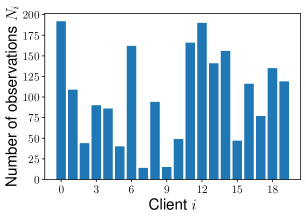
Figure S1: Illustration of the unbalancedness of the synthetic dataset used in the Toy Gaussian experiment.

To obtain the figure at the bottom row of Figure 1 in the main paper, we launched all the MCMC algorithms with $K=500,000$ outer iterations and considered a burn-in period of $450,000$ iterations. Hence, only the last $50,000$ samples have been used to compute the MSE associated to the test function $f:\theta\mapsto\left\|{\theta}\right\|$. In order to compute the expected number of bits transmitted during each upload period, we considered the Elias encoding scheme and used the upper-bounds given in Alistarh et al. (2017, Theorem 3.2 and Lemma A.2).

• License of the assets: No existing asset has been used for this experiment.

• Total amount of compute and type of resources used: This experiment has been run on a laptop running Windows 10 and equipped with Intel(R) Core(TM) i7_8565U CPU 1.80GHz with 16Go of RAM. The total amount of compute is roughly 33 hours.

• Training details: All training details (here hyperparameters) are detailed in Section 4 in the main paper.

Discretisation step-size and compression trade-off. We complement the analysis made in the main paper by showing on Figure S2 that the saving in terms of number of transmitted bits can be further improved by decreasing the value of $\gamma$. This numerical finding illustrates our theory which in particular shows that the asymptotic bias associated to $\texttt{QLSD}^{\star}$ is of the order $\omega\operatorname{\mathrm{O}}(\gamma)$, see Table 1 in the main paper.

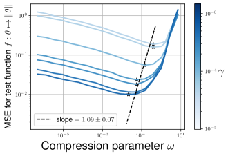
Figure S2: Toy Gaussian example. Trade-off between step-size and compression parameter values.

S5.2 Bayesian logistic regression

Pseudo-code of LSD⁺⁺. For completeness, we provide in Algorithm S3 the pseudo-code of the non-compressed counterpart of QLSD⁺⁺, namely LSD⁺⁺.

Algorithm S3 Variance-reduced Langevin Stochastic Dynamics (LSD⁺⁺)

Input: minibatch sizes $\{n_{i}\}_{i\in[b]}$, number of iterations $K$, step-size $\gamma\in(0,\bar{\gamma}]$ with $\bar{\gamma}>0$, initial point $\theta_{0}$ and $\alpha\in(0,\bar{\alpha}]$ with $\bar{\alpha}>0$.

// Memory mechanism initialisation

Initialise $\{\eta^{(1)}_{0},\ldots,\eta^{(b)}_{0}\}$ and $\eta_{0}=\sum_{i=1}^{b}\eta^{(i)}_{0}$.

for $k=0$ to $K-1$ do

      // Update of the control variates

     if $k\equiv 0$ ($\mathrm{mod}\ l$) then

         Set $\zeta_{k}=\theta_{k}$.

     else

         Set $\zeta_{k}=\zeta_{k-1}$

     end if

     for $i\in\mathcal{A}_{k+1}$ // On active clients do

         Draw $\mathcal{S}_{k+1}^{(i)}\sim\mathrm{Uniform}\left({\wp_{N_{i},n_{i}}}\right)$.

         Set $H_{k+1}^{(i)}(\theta_{k})=(N_{i}/n_{i})\sum_{j\in\mathcal{S}_{k+1}^{(i)}}[\nabla U_{i,j}(\theta_{k})-\nabla U_{i,j}(\zeta_{k})]+\nabla U_{i}(\zeta_{k})$.

         Compute $\textsl{g}_{i,k+1}=H_{k+1}^{(i)}(\theta_{k})-\eta^{(i)}_{k}$.

         Send $\textsl{g}_{i,k+1}$ to the central server.

         Set $\eta^{(i)}_{k+1}=\eta^{(i)}_{k}+\alpha\textsl{g}_{i,k+1}$.

     end for

      // On the central server

     Compute $\textsl{g}_{k+1}=\eta_{k}+\frac{b}{|\mathcal{A}_{k+1}|}\sum_{i\in\mathcal{A}_{k+1}}\textsl{g}_{i,k+1}$.

     Set $\eta_{k+1}=\eta_{k}+\alpha\sum_{i\in\mathcal{A}_{k+1}}^{b}\textsl{g}_{i,k+1}$.

     Draw $Z_{k+1}\sim\mathrm{N}(0_{d},\mathrm{I}_{d})$.

     Compute $\theta_{k+1}=\theta_{k}-\gamma\textsl{g}_{k+1}+\sqrt{2\gamma}Z_{k+1}$.

     Send $\theta_{k+1}$ to the $b$ clients.

end for

Output: samples $\{\theta_{k}\}_{k=0}^{K}$.

Additional experimental details. The code associated to this experiment can be found in the supplementary material (see ./code/notebook_logistic_regression.ipynb). For the Bayesian logistic regression experiment detailed in the main paper, we ran the MCMC algorithms with $K=500,000$ outer iterations and considered a burn-in period of length $50,000$.

Benefits of the memory mechanism. We also run an additional experiment on a low-dimensional synthetic dataset to highlight the benefits brought by the memory mechanism involved in QLSD⁺⁺ when the dataset is highly heterogeneous. To this end, we consider the Synthetic$(\alpha,\beta)$ dataset (Li et al., 2020) with $\alpha=\beta=1$, $d=2$ and $b=50$. We run QLSD⁺⁺ with and without memory terms using $l=100$, $\alpha=1/(\omega+1)$, $\gamma=10^{-5}$ and for huge compression parameters, namely $s\in\{2^{1},2^{2}\}$. We use $K=100,000$ outer iterations without considering a burn-in period. In order to have access to some ground truth, we also implement the Metropolis-adjusted Langevin algorithm (MALA) (Robert and Casella, 2004).

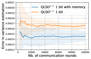
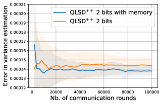
Figure S3: Bayesian logistic regression on synthetic data.

Figure S3 shows the Euclidean norm of the error between the true variance under $\pi$ estimated with MALA and the empirical variance computed using samples generated by QLSD⁺⁺. As expected, we can notice that the memory mechanism reduces the impact of the compression on the asymptotic bias of QLSD⁺⁺ when $\omega$ is large.

Results on a non-image dataset. In order to complement our results on an image dataset (FEMNIST), we also implement our methodology and one competitor (DG-SGLD) on the covtype dataset. Again, the ground truth has been obtained by implementing a long-run Metropolis-adjusted Langevin algorithm. The results we obtained are gathered in Table S1.

Table S1: Bayesian Logistic Regression on covtype dataset.

Algorithm	99% HPD error
DG-SGLD	1.8e-2
QLSD++ 4 bits	2.2e-3
QLSD++ 8 bits	2.0e-2
QLSD++ 16 bits	1.9e-2

• License of the assets: We use the Synthetic dataset whose associated code is under the MIT license, and the FEMNIST dataset whose data are publicy available and associated code is under MIT license.

• Total amount of compute and type of resources used: This experiment has been run on a laptop running Windows 10 and equipped with Intel(R) Core(TM) i7_8565U CPU 1.80GHz with 16Go of RAM. The total amount of compute is roughly 30 hours.

• Training details: Hyperparameter values are detailed in Section 4 in the main paper. Regarding our experiment on real data, we use a random subset of the initial training data (for computational reasons).

S5.3 Bayesian neural networks

• License of the assets: We use the MNIST, FMNIST, CIFAR10 and SVHN datasets which are publicly downloadable with the torchvision.datasets package.

• Total amount of compute and type of resources used: The total computational cost depends on the dataset, but is roughly 40 hours in the worst case.

• Training details: We consider the same hyperparameter values detailed in Table S2 for both training on MNIST and CIFAR10 except for the initialisation and the sampling period. For the MNIST dataset, we use the default random weights given by pytorch whereas for CIFAR-10 we use the warm-start provided by the pytorchcv library and consider a burn-in period of half the sampling period ($K=10^{4}$ iterations) with a thinning of 10.

In the following, we denote $\mathrm{D}_{\text{test}}$ the test dataset and for any data $(x,y)\in\mathrm{D}_{\text{test}}$, we define the preditive density by

$$p(y\mid x)=\int p(y\mid x,\theta)\ \pi(\theta\mid\mathrm{D})\ \mathrm{d}\theta\,,$$ (S84)

where $p(y\mid x,\theta)$ is the conditional likelihood. For any input $x$, the predicted label is denoted by $y_{\mathrm{pred}}(x)=\operatorname*{arg\,max}_{y}p(y\mid x)$.

Metrics used for the Bayesian neural network experiment in the main paper. In the main paper, we consider three metrics to compare the different Bayesian FL algorithms, namely Accuracy, Agreement and TV. They are defined in the following.

• Accuracy: Based on samples from the approximate posterior distribution, we compute the minimum mean-square estimator (i.e. corresponding to the posterior mean) and use it to make predictions on the test dataset. The Accuracy metric corresponds to the percentage of well-predicted labels.

• Agreement: Let denote $p_{\mathrm{ref}}$ and $p$ the predictive densities associated to HMC and an approximate simulation-based algorithm, respectively. Similar to Izmailov et al. (2021), we define the agreement between $p_{\mathrm{ref}}$ and $p$ as the fraction of the test datapoints for which the top-1 predictions of $p_{\mathrm{ref}}$ and $p$, i.e.

  $$\mathrm{agreement}(p_{\mathrm{ref}},p)=\frac{1}{|\mathrm{D}_{\mathrm{test}}|}\sum_{x\in\mathrm{D}_{\mathrm{test}}}\mathbf{1}\left\{{\operatorname*{arg\,max}_{y^{\prime}}p_{\mathrm{ref}}(y^{\prime}\mid x)=\operatorname*{arg\,max}_{y^{\prime}}p(y^{\prime}\mid x)}\right\}\,.$$

• Total variation (TV): By denoting $\mathcal{Y}$ the set of possible labels, we consider the total variation metric between $p_{\mathrm{ref}}$ and $p$, i.e.

  $$\mathrm{TV}(p_{\mathrm{ref}},p)=\frac{1}{2|\mathrm{D}_{\mathrm{test}}|}\sum_{x\in\mathrm{D}_{\mathrm{test}}}\sum_{y^{\prime}\in\mathcal{Y}}\left|p_{\mathrm{ref}}(y^{\prime}\mid x)-p(y^{\prime}\mid x)\right|\,.$$

Performance results on a highly heterogeneous dataset. We train LeNet5 (LeCun et al., 1998) architecture on the MNIST dataset (Deng, 2012) and we consider the FMNIST (Xiao et al., 2017) as the out-of-distribution dataset. To obtain a highly heterogeneous setting, we split the data among $b=20$ clients so that each client has a dominant label representing $40\%$ of the total amount in the training set and $1\%$ of the other labels as described in Figure S4.

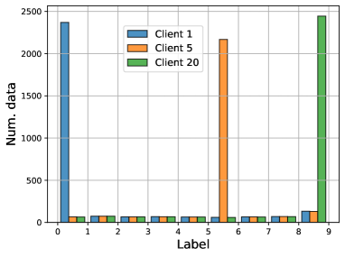
Figure S4: Number of labels owned by different clients.

Inspired by the scores defined in Guo et al. (2017), we measure the performance of the different algorithms and report those results in Table S2. These statistics aim to better understand the predictions in order to calibrate the models (Rahaman and Thiery, 2020).

Method	SGLD	pSGLD	QLSD	QLSD PP	QLSD++	QLSD++ PP	FedBe-Gauss.	FedBe-Dirich.	FSGLD
Accuracy	99.1	99.2	98.8	98.3	98.8	98.7	43.5	79.3	98.5
$10^{2}\times$ ECE	0.577	1.25	0.916	1.57	0.692	0.930	7.51	21.3	2.65
$10^{2}\times$ BS	1.38	1.39	1.98	2.23	1.91	2.18	66.6	36.1	2.64
$10^{2}\times$ nNLL	2.86	3.16	4.15	4.82	4.11	4.65	139	78.0	6.19
Weight Decay	5	5	5	5	5	5	0	0	5
Batch Size	64	64	64	64	64	64	64	64	64
Learning rate	1e-07	1e-08	1e-07	1e-07	1e-07	1e-07	1e-02	1e-02	1e-07
Local steps	N/A	N/A	1	1	1	1	250	250	16
Burn-in	100epch.	100epch.	1e04	1e04	1e04	1e04	N/A	N/A	1e04
Thinning	1	1	500	500	500	500	N/A	N/A	500
Training	1e03epch.	1e03epch.	1e05it.	1e05it.	1e05it.	1e05it.	N/A	N/A	1e05it.

Table S2: Performance of Bayesian FL algorithms trained on the highly-heterogeneous dataset.

Expected Calibration Error (ECE).

To measure the difference between the accuracy and confidence of the predictions, we group the data into $M\geq 1$ buckets defined for any $m\in[M]$ by $\mathrm{B_{m}}=\{(x,y)\in\mathrm{D}_{\mathrm{test}}:p(y_{\mathrm{pred}}(x)|x)\in\left]{(m-1)}/{M},{m}/{M}\right]\}$. As in the previous work of Ovadia et al. (2019), we denote the model accuracy on $\mathrm{B_{m}}$ by

$$\mathrm{acc}\left(\mathrm{B_{m}}\right)=\frac{1}{\left|\mathrm{B_{m}}\right|}\sum_{(x,y)\in\mathrm{B_{m}}}\mathbf{1}_{y_{\mathrm{pred}}(x)=y}$$

and define the confidence on $\mathrm{B_{m}}$ by

$$\mathrm{conf}\left(\mathrm{B_{m}}\right)=\frac{1}{\left|\mathrm{B_{m}}\right|}\sum_{(x,y)\in\mathrm{B_{m}}}p(y_{\mathrm{pred}}(x)|x)\,.$$

As stressed in Guo et al. (2017), for any $m\in[M]$ the accurcay $\mathrm{acc}\left(\mathrm{B_{m}}\right)$ is an unbiased and consistent estimator of $\mathbb{P}\left(y_{\mathrm{pred}}(x)=y\mid(m-1)/M<p(y_{\mathrm{pred}}(x)|x)\leq{m}/{M}\right)$. Therefore, the ECE defined by

$$\mathrm{ECE}=\sum_{m=1}^{M}\frac{\left|\mathrm{B_{m}}\right|}{\left|\mathrm{D}_{\mathrm{test}}\right|}\left|\mathrm{acc}\left(\mathrm{B_{m}}\right)-\mathrm{conf}\left(\mathrm{B_{m}}\right)\right|$$

is an estimator of

$$\mathbb{E}_{(x,y)}\Big{[}\big{|}\mathbb{P}\left({y_{\mathrm{pred}}(x)=y\mid p(y_{\mathrm{pred}}(x)|x)}\right)-p(y_{\mathrm{pred}}(x)|x)\big{|}\Big{]}.$$

Thus, ECE measures the absolute difference between the confidence level of a prediction and its accuracy.

Brier Score (BS).

The BS is a proper scoring rule (see for example Dawid and Musio (2014)) that can only evaluate random variables taking a finite number of values. Denote by $\mathcal{Y}$ the finite set of possible labels, the BS measures the model’s confidence in its predictions and is defined by

$$\mathrm{BS}=\frac{1}{|\mathrm{D}_{\mathrm{test}}|}\sum_{(x,y)\in\mathrm{D}_{\mathrm{test}}}\sum_{c\in\mathcal{Y}}(p(y=c|x)-\mathbf{1}_{y=c})^{2}\,.$$

Normalised negative log-likelihood (nNLL).

This classical score defined by

$$\mathrm{nNLL}=-\frac{1}{|\mathrm{D}_{\mathrm{test}}|}\sum_{(x,y)\in\mathrm{D}_{\mathrm{test}}}\log p(y|x)$$

measures the model ability to predict good labels with high probability.

Out of distribution detection.

Here we study the behavior of our proposed algorithms in the out-of-distribution (OOD) framework, we consider the pairs MNIST/FMNIST and CIFAR10/SVHN, comparing the densities of the predictive entropies on the ID vs OOD data. These densities denoted by $p_{\text{in}}$ and $p_{\text{out}}$ respectively, are approximated using a kernel estimator based on of the histogram associated with $\{\mathrm{Ent}(x):x\in\mathrm{D}_{\mathrm{test}}^{x}\}$ for $\mathrm{D}_{\mathrm{test}}\in\{\text{MNIST},\text{FMNIST}\}$ or $\{\text{CIFAR10},\text{SVHN}\}$, where $\mathrm{Ent}(x)$ is the predictive entropy defined by:

$$\mathrm{Ent}(x)=\sum_{y\in\mathcal{Y}}p(y|x)\log p(y|x)\,,$$

and $p(y|x)$ is defined by (S84) and estimated by the different methods that we consider. The resulting densities from the different methods that we consider are displayed in Figure S5.

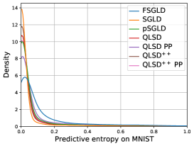
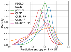
Figure S5: Predictive entropies comparison between MNIST and FMNIST.

A new data point $x$ is then labeled in the original dataset (MNIST or CIFAR10) if $p_{\text{in}}(\mathrm{Ent}(x))>p_{\text{out}}(\mathrm{Ent}(x))$ and out-of-distribution otherwise.

Calibration results.

Interpreting the predicted outputs as probabilities is only correct for well a calibrated model. Indeed, when a model is calibrated, the confidence is closed to the accuracy of the predictions. In order to evaluate the calibration of the models, we display the reliability diagram on the left-hand side of Figure S6. It represents the evolution of $\mathrm{acc}(\mathrm{B_{m}})-\mathrm{conf}(\mathrm{B_{m}})$ in function of $\mathrm{conf}(\mathrm{B_{m}})$, closer the values are to zero better the model is calibrated.

For the second sub-experiment, we consider for any $\tau\in[{\textstyle{0,1}}]$, the set $\mathrm{D}_{\mathrm{pred}}^{(\tau)}=\{x\in\mathrm{D}_{\mathrm{test}}^{x}:p(y|x)\geq\tau\}$ of classified data with credibility greater than $\tau$. We define the test accuracy on $\mathrm{D}_{\mathrm{pred}}^{(\tau)}$ by

$$\mathrm{Card}(\{x\in\mathrm{D}_{\mathrm{pred}}^{(\tau)}:y_{\mathrm{true}}(x)=y_{\mathrm{pred}}(x)\})/\mathrm{Card}(\mathrm{D}_{\mathrm{pred}}^{(\tau)})\,.$$

The right-hand side of Figure S6 shows the evolution of the test accuracy on $\mathrm{D}_{\mathrm{pred}}^{(\tau)}$ with respect to the credibility threshold $\tau$. It can be noted that in both plots of Figure S6, the accuracy tends to $100\%$ for confident predictions.

Figure S6: Left: Calibration test from reliability diagrams – Right: Test accuracy on $\mathrm{D}_{\mathrm{pred}}^{(\tau)}$ with respect to the threshold $\tau$.

References

- Ahn et al. (2014) Sungjin Ahn, Babak Shahbaba, and Max Welling. Distributed Stochastic Gradient MCMC. In International Conference on Machine Learning, 2014.
- Aji and Heafield (2017) Alham Fikri Aji and Kenneth Heafield. Sparse Communication for Distributed Gradient Descent. In Conference on Empirical Methods in Natural Language Processing, 2017.
- Alistarh et al. (2017) Dan Alistarh, Demjan Grubic, Jerry Li, Ryota Tomioka, and Milan Vojnovic. QSGD: Communication-efficient SGD via gradient quantization and encoding. Advances in Neural Information Processing Systems, 2017.
- Andrieu et al. (2003) Christophe Andrieu, Nando de Freitas, Arnaud Doucet, and Michael I. Jordan. An introduction to MCMC for machine learning. Machine Learning, 50(1–2):5–43, 2003.
- Baker et al. (2019) Jack Baker, Paul Fearnhead, Emily B. Fox, and Christopher Nemeth. Control variates for stochastic gradient MCMC. Statistics and Computing, 29(3):599–615, 2019.
- Brosse et al. (2018) Nicolas Brosse, Alain Durmus, and Eric Moulines. The promises and pitfalls of Stochastic Gradient Langevin Dynamics. In Advances in Neural Information Processing Systems, 2018.
- Bui et al. (2018) Thang D. Bui, Cuong V. Nguyen, Siddharth Swaroop, and Richard E. Turner. Partitioned Variational Inference: A unified framework encompassing federated and continual learning. arXiv preprint arXiv:1811.11206, 2018.
- Caldas et al. (2018) Sebastian Caldas, Sai Meher Karthik Duddu, Peter Wu, Tian Li, Jakub Konecny, H. Brendan McMahan, Virginia Smith, and Ameet Talwalkar. LEAF: A Benchmark for Federated Settings. arXiv preprint arXiv:1812.01097, 2018.
- Chen and Chao (2021) Hong-You Chen and Wei-Lun Chao. FedBE: Making Bayesian Model Ensemble Applicable to Federated Learning. In International Conference on Learning Representations, 2021.
- Corinzia et al. (2019) Luca Corinzia, Ami Beuret, and Joachim M. Buhmann. Variational Federated Multi-Task Learning. arXiv preprint arXiv:1906.06268, 2019.
- Dalalyan (2017) Arnak S. Dalalyan. Theoretical guarantees for approximate sampling from smooth and log-concave densities. Journal of the Royal Statistical Society, Series B, 79(3):651–676, 2017.
- Dalalyan and Karagulyan (2019) Arnak S. Dalalyan and Avetik Karagulyan. User-friendly guarantees for the Langevin Monte Carlo with inaccurate gradient. Stochastic Processes and Their Applications, 129(12):5278–5311, 2019.
- Dawid and Musio (2014) Alexander Philip Dawid and Monica Musio. Theory and applications of proper scoring rules. Metron, 72(2):169–183, 2014.
- Deng (2012) Li Deng. The mnist database of handwritten digit images for machine learning research. IEEE Signal Processing Magazine, 29(6):141–142, 2012.
- Dieuleveut et al. (2020) Aymeric Dieuleveut, Alain Durmus, and Francis Bach. Bridging the gap between constant step size stochastic gradient descent and Markov chains. Annals of Statistics, 48(3):1348–1382, 06 2020.
- Durmus and Moulines (2019) Alain Durmus and Eric Moulines. High-dimensional Bayesian inference via the unadjusted Langevin algorithm. Bernoulli, 25(4A):2854–2882, 2019.
- Durmus et al. (2019) Alain Durmus, Szymon Majewski, and Blażej Miasojedow. Analysis of Langevin Monte Carlo via convex optimization. Journal of Machine Learning Research, 20(73):1–46, 2019.
- El Mekkaoui et al. (2021) Khaoula El Mekkaoui, Diego Mesquita, Paul Blomstedt, and Samuel Kaski. Distributed stochastic gradient MCMC for federated learning. In Conference on Uncertainty in Artificial Intelligence, 2021.
- Franchi et al. (2020) Gianni Franchi, Andrei Bursuc, Emanuel Aldea, Severine Dubuisson, and Isabelle Bloch. Encoding the latent posterior of Bayesian Neural Networks for uncertainty quantification. arXiv preprint arXiv:2012.02818, 2020.
- Girgis et al. (2020) Antonious M Girgis, Deepesh Data, Suhas Diggavi, Peter Kairouz, and Ananda Theertha Suresh. Shuffled model of federated learning: Privacy, communication and accuracy trade-offs. arXiv preprint arXiv:2008.07180, 2020.
- Grenander and Miller (1994) Ulf Grenander and Michael I. Miller. Representations of knowledge in complex systems. Journal of the Royal Statistical Society, Series B, 56(4):549–603, 1994.
- Guo et al. (2017) Chuan Guo, Geoff Pleiss, Yu Sun, and Kilian Q Weinberger. On calibration of modern neural networks. In International Conference on Machine Learning, pages 1321–1330. PMLR, 2017.
- Haddadpour et al. (2020) Farzin Haddadpour, Mohammad Mahdi Kamani, Aryan Mokhtari, and Mehrdad Mahdavi. Federated Learning with Compression: Unified Analysis and Sharp Guarantees. arXiv preprint arXiv:2007.01154, 2020.
- Hasenclever et al. (2017) Leonard Hasenclever, Stefan Webb, Thibaut Lienart, Sebastian Vollmer, Balaji Lakshminarayanan, Charles Blundell, and Yee Whye Teh. Distributed Bayesian Learning with Stochastic Natural Gradient Expectation Propagation and the Posterior Server. Journal of Machine Learning Research, 18(106):1–37, 2017.
- He et al. (2016) Kaiming He, Xiangyu Zhang, Shaoqing Ren, and Jian Sun. Deep residual learning for image recognition. In IEEE Conference on Computer Vision and Pattern Recognition, pages 770–778, 2016.
- Hoffman et al. (2013) Matthew D. Hoffman, David M. Blei, Chong Wang, and John Paisley. Stochastic Variational Inference. Journal of Machine Learning Research, 14(4):1303–1347, 2013.
- Horváth et al. (2019) Samuel Horváth, Dmitry Kovalev, Konstantin Mishchenko, Sebastian Stich, and Peter Richtárik. Stochastic Distributed Learning with Gradient Quantization and Variance Reduction . arXiv preprint arXiv:1904.05115, 2019.
- Hunter (2016) David J. Hunter. Uncertainty in the Era of Precision Medicine. New England Journal of Medicine, 375(8):711–713, 2016.
- Izmailov et al. (2020) Pavel Izmailov, Wesley J Maddox, Polina Kirichenko, Timur Garipov, Dmitry Vetrov, and Andrew Gordon Wilson. Subspace inference for Bayesian deep learning. In Uncertainty in Artificial Intelligence, pages 1169–1179, 2020.
- Izmailov et al. (2021) Pavel Izmailov, Sharad Vikram, Matthew D Hoffman, and Andrew Gordon Wilson. What Are Bayesian Neural Network Posteriors Really Like? arXiv preprint arXiv:2104.14421, 2021.
- Johnson and Zhang (2013) Rie Johnson and Tong Zhang. Accelerating Stochastic Gradient Descent Using Predictive Variance Reduction. In Advances in Neural Information Processing Systems, page 315–323, 2013.
- Jordan et al. (2019) Michael I. Jordan, Jason D. Lee, and Yun Yang. Communication-Efficient Distributed Statistical Inference. Journal of the American Statistical Association, 114(526):668–681, 2019.
- Kairouz et al. (2021) Peter Kairouz, H. Brendan McMahan, Brendan Avent, Aurélien Bellet, Mehdi Bennis, Arjun Nitin Bhagoji, K. A. Bonawitz, Zachary Charles, Graham Cormode, Rachel Cummings, Rafael G.L. D’Oliveira, Salim El Rouayheb, David Evans, Josh Gardner, Zachary Garrett, Adrià Gascón, Badih Ghazi, Phillip B. Gibbons, Marco Gruteser, Zaid Harchaoui, Chaoyang He, Lie He, Zhouyuan Huo, Ben Hutchinson, Justin Hsu, Martin Jaggi, Tara Javidi, Gauri Joshi, Mikhail Khodak, Jakub Konevcný, Aleksandra Korolova, Farinaz Koushanfar, Sanmi Koyejo, Tancrède Lepoint, Yang Liu, Prateek Mittal, Mehryar Mohri, Richard Nock, Ayfer Özgür, Rasmus Pagh, Mariana Raykova, Hang Qi, Daniel Ramage, Ramesh Raskar, Dawn Song, Weikang Song, Sebastian U. Stich, Ziteng Sun, Ananda Theertha Suresh, Florian Tramèr, Praneeth Vepakomma, Jianyu Wang, Li Xiong, Zheng Xu, Qiang Yang, Felix X. Yu, Han Yu, and Sen Zhao. Advances and Open Problems in Federated Learning. Foundations and Trends in Machine Learning, 14(1–2):1–210, 2021.
- Karimireddy et al. (2020) Sai Praneeth Karimireddy, Satyen Kale, Mehryar Mohri, Sashank Reddi, Sebastian Stich, and Ananda Theertha Suresh. SCAFFOLD: Stochastic Controlled Averaging for Federated Learning. In International Conference on Machine Learning, 2020.