Quadrature for Implicitly-defined Finite Element Functions on Curvilinear Polygons

Abstract.

$H^{1}$-conforming Galerkin methods on polygonal meshes such as VEM, BEM-FEM and Trefftz-FEM employ local finite element functions that are implicitly defined as solutions of Poisson problems having polynomial source and boundary data. Recently, such methods have been extended to allow for mesh cells that are curvilinear polygons. Such extensions present new challenges for determining suitable quadratures. We describe an approach for integrating products of these implicitly defined functions, as well as products of their gradients, that reduces integrals on cells to integrals along their boundaries. Numerical experiments illustrate the practical performance of the proposed methods.

1. Introduction

The construction, analysis and implementation of finite element methods employing meshes consisting of non-standard cell shapes (e.g. fairly general polygons in 2D and polyhedra in 3D) have generated a lot of interest, and a sizable literature, in the last 10+ years. We do not attempt here to provide a representative sample of the literature, but instead highlight three closely-related approaches for second-order (linear) elliptic problems that yield $H^{1}$-conforming finite element spaces, and provide motivation for the problems considered in this work. Virtual Element Methods (VEM) (cf. [11, 1, 16, 12, 14, 4, 20, 13, 15, 6, 5, 10, 9]), Boundary Element-Based Finite Element Methods (BEM-FEM) (cf. [39, 32, 33, 40, 26, 41, 44, 43, 42, 34]) and Trefftz-type Finite Element Methods (Trefftz-FEM) (cf. [18, 25, 24, 3, 2]) all employ vector spaces that are implicitly defined, as in (1). The primary difference between VEM on the one hand, and BEM-FEM and Trefftz-FEM on the other, is how they work with such implicitly defined spaces in practice, particularly with regard to forming finite element linear systems. In VEM, the space is treated “virtually” via degrees of freedom that provide enough information, up to a well-chosen stabilization term, to form the linear system; computations with basis functions (shape functions) are avoided. In contrast, BEM-FEM and Trefftz-FEM work more directly with basis functions, which are defined implicitly in terms of Poisson problems with explicitly given (polynomial) data. All computations involving these basis functions (e.g. pointwise evaluation of functions and some of their derivatives) are carried out using the solution of associated boundary integral equations. BEM-FEM and Trefftz-FEM differ primarily in the types of boundary integral equations that are solved (typically second-kind for Trefftz-FEM, and first-kind for BEM-FEM), and the discretizations employed for solving them (Nyström methods for recent versions of Trefftz-FEM, and BEM for BEM-FEM). Recently, Trefftz-FEM and VEM have been extended to allow for mesh cells that are curvilinear polygons (cf.[3, 10, 2, 9]).

Determining suitable quadratures for finite elements on general polytopal meshes is clearly more challenging than for standard meshes, such as those involving only simplices and/or basic (affine) transformations of tensor product cells, for which polynomial-based quadratures of high order are readily available. Allowing for general curvilinear polygons and non-polynomial functions further complicates the matter. An obvious approach to quadrature on polytopes is to first partition it into such standard mesh cells, apply the known quadratures on each, and sum the result. This “brute-force” approach, though costly, remains popular because of the simplicity of its implementation. It is used, for example, in the BEM-FEM literature, whenever higher-order spaces, e.g. (1) for $m>1$, are employed. Making no attempt at being exhaustive, we briefly describe some of the more sophisticated approaches—the introduction in [7] provides a good starting point for a more detailed exploration. In [35], the authors describe an approach yielding Gauss-like quadratures for polygons, which are exact for polynomials of a given degree $2n-1$. An unattractive feature of the approach is that it often leads to quadrature points that lie outside the polygon. However, in many cases, including all convex polygons, a modified version of their approach yields all quadrature points in the polygon. In [36], the authors propose a similar approach which also allows for integration on polyhedra, and provide a more careful reporting of its practical efficiency. In [30], the authors first use a Schwarz-Christoffel (conformal) mapping to transform a polygon to the unit disk, which is clearly tensorial in polar coordinates, and then any number of basic 1D quadratures (e.g. midpoint rule) may be applied in the radial and angular directions. The authors discuss numerical methods for determining the conformal map for each polygon. A more sophisticated subpartitioning approach is described in [38], with the aim of integrating non-polynomial (often rational) functions such as several variants of “generalized barycentric coordinates” naturally arising in Polygonal FEM (PFEM) (cf. [19, 27]). The contribution [37] describes methods for systematically “compressing” pre-existing quadrature rules, keeping a subset of the original nodes and recomputing quadrature weights, in order to retain as much of the effectiveness of the original quadrature while often drastically reducing the number of quadrature nodes. In [7], the authors consider the integration of polynomials on (flat-faced) polytopes in $\mathbb{R}^{d}$. A simple identity for homogeneous functions allows recursive reduction of the integral of a polynomial on the polytope to a sum of integrals lower-dimensional facets, ending in evaluation at the vertices. The first step in their reduction can also be used for curvilinear polygons, so we provide further details in Section 3. A very recent contribution [8] considers quadratures on curvilinear polygons whose curved edges are arcs of circles, and whose vertices are also the vertices of a convex polygon. This approach first partitions the cell into (curved) triangles and rectangles, each having at most once curved edge, generates quadratures for these specialized shapes, and then sums them to obtain a quadrature for the entire cell. Finally, a compression technique is used to reduce the number of quadrature points.

Given $m\in\mathbb{Z}$, we denote by $\mathbb{P}_{m}$ the vector space of (real-valued) polynomials of total degree $\leq m$ on $\mathbb{R}^{2}$, with the convention that $\mathbb{P}_{m}=\{0\}$ when $m<0$. We recall that $\dim\mathbb{P}_{m}=\binom{m+2}{2}$. For non-empty $S\subset\mathbb{R}^{2}$, we define $\mathbb{P}_{m}(S)$ as the restriction of $\mathbb{P}_{m}$ to $S$, and note that it is also a vector space. The dimension of $\mathbb{P}_{m}(S)$ depends on the nature of $S$. For example, if $S$ is open and connected, then $\dim\mathbb{P}_{m}(S)=\dim\mathbb{P}_{m}=\binom{m+2}{2}$; if $S$ consists of a single point, then $\dim\mathbb{P}_{m}(S)=1$; if $S$ is a straight line or a segment thereof, then $\dim\mathbb{P}_{m}(S)=\binom{m+2}{2}-\binom{m+1}{2}=m+1$; and if $S$ is an arc of a curved conic section, then $\dim\mathbb{P}_{m}(S)=\binom{m+2}{2}-\binom{m}{2}$. Further discussion of $\mathbb{P}_{m}(e)$, where $e$ is a simple (bounded) curve, is given in [2].

Let $K\subset\mathbb{R}^{2}$ be open, bounded, simply connected, whose Lipschitz boundary $\partial K$ is a union of smooth arcs with disjoint interiors, which we call edges. We refer to $K$ as a curvilinear polygon. Points where adjacent edges meet are called vertices, and adjacent edges are allowed to meet at a straight angle. For $m\in\mathbb{N}$, we define $\mathbb{P}_{m}^{*}(\partial K)$ to be the vector space of continuous functions on $\partial K$ such that the restriction of such a function to an edge $e$ of $K$ is in $\mathbb{P}_{m}(e)$. It is clear that $\mathbb{P}_{m}(\partial K)\subset\mathbb{P}_{m}^{*}(\partial K)$. We define the space $V_{m}(K)$ as

(1) $$V_{m}(K)=\{v\in H^{1}(K):\,\Delta v\in\mathbb{P}_{m-2}(K)\mbox{ in }K\,,\,v_{|_{\partial K}}\in\mathbb{P}_{m}^{*}(\partial K)\}~{}.$$

It is apparent from the definition that $\mathbb{P}_{m}(K)\subset V_{m}(K)$, and it can be shown that the only way in which equality is achieved is when $m=1$ and $K$ is a triangle. A natural decomposition of $V_{m}(K)$ is $V_{m}(K)=V_{m}^{\partial K}(K)\oplus V_{m}^{K}(K)$, where

(2a) $$V^{\partial K}_{m}(K) =\{v\in H^{1}(K):\,\Delta v=0\mbox{ in }K\,,\,v_{|_{\partial K}}\in\mathbb{P}_{m}^{*}(\partial K)\}~{},$$

(2b) $$V^{K}_{m}(K) =\{v\in H^{1}(K):\,\Delta v\in\mathbb{P}_{m-2}(K)\mbox{ in }K\,,\,v_{|_{\partial K}}=0\}~{}.$$

We see that $\dim V^{K}_{m}(K)=\dim\mathbb{P}_{m-2}(K)=\binom{m}{2}$, and that $\dim V^{\partial K}_{m}(K)=\dim\mathbb{P}_{m}^{*}(\partial K)$, the latter of which not only depends on $m$, but also on the number and nature of the edges of $K$.

We consider methods for efficiently approximating integrals of the forms

(3) $$\int_{K}vw\,dx\quad,\quad\int_{K}\nabla v\cdot\nabla w\,dx~{},$$

for $v,w\in V_{m}(K)$, by reducing the computations to integrals along the boundary $\partial K$. As we will see in subsequent sections, we will never need to evaluate functions or their gradients in the interior of $K$ in order to evaluate the integrals in (3) for $v,w\in V_{m}(K)$. We will only need access to Dirichlet and Neumann traces of associated functions.

The rest of the paper is organized as follows. In Section 2, we discuss algebraic and computational techniques for determining functions whose Laplacian is either a polynomial or a harmonic function. Using these, we describe how the integrals (3) can be reduced to associated integrals on cell boundaries. Quadratures along the edges require evaluation of associated functions and their normal derivatives, which are provided algebraically for polynomials and via boundary integral equations for harmonic functions. Numerical experiments illustrating the practical performance of the approach are provided in Section 4. Section 5 contains further details, such as our chosen quadrature for edges, that are not as central to the discussion and would unnecessarily bog down the reading of the paper if they were included earlier.

2. Preliminary Results

It will be useful to have techniques for solving Poisson problems having polynomial or harmonic source terms. The following result is a corollary of [28, Theorem 2].

Proposition 2.1.

Suppose $p\in\mathbb{P}_{n}$. There is a $P\in\mathbb{P}_{n+2}$ such that $\Delta P=p$. More explicitly, if $p(x)=\sum_{|\alpha|\leq n}c_{\alpha}(x-z)^{\alpha}$, then we may choose

(4) $$P(x)=\sum_{|\alpha|\leq n}c_{\alpha}P_{\alpha}(x)\quad,\quad P_{\alpha}(x)=\frac{|x-z|^{2}}{4(|\alpha|+1)!}\sum_{k=0}^{\lfloor|\alpha|/2\rfloor}\frac{(-1)^{k}(|\alpha|-k)!}{(k+1)!}\left(\frac{|x-z|^{2}}{4}\right)^{k}\Delta^{k}(x-z)^{\alpha}~{},$$

where $\lfloor s\rfloor$ is the integer part of $s$.

We note that $P_{\alpha}$, which satisfies $\Delta P_{\alpha}=(x-z)^{\alpha}$, is homogeneous of degree $|\alpha|+2$, and that these polynomials may be computed offline and tabulated for $|\alpha|$ up to some specified threshold, so that $P$ may be computed efficiently from the coefficients $c_{\alpha}$ of $p$. A polynomial $q\in\mathbb{P}_{j}$ given with respect to a shifted monomial basis, as is $p$ above, can be encoded as a coefficient array of length $J=\binom{j+2}{2}$, once a suitable enumeration of the multiindices $\alpha$ is chosen. Such an enumeration is given in Table 1 for $|\alpha|\leq 6$, and its extension to all multiindices is clear.

Table 1. An enumeration of multiindices for $|\alpha|\leq 6$, together with the indices and values of the non-zero coefficients of $P_{\alpha}$ from Proposition 2.1.

$k$	$\alpha$	$P_{\alpha}$ indices	$P_{\alpha}$ coefficients
0	$(0,0)$	$(3,5)$	$(1,1)/4$
1	$(1,0)$	$(6,8)$	$(1,1)/8$
2	$(0,1)$	$(7,9)$	$(1,1)/8$
3	$(2,0)$	$(10,12,14)$	$(7,6,-1)/96$
4	$(1,1)$	$(11,13)$	$(1,1)/12$
5	$(0,2)$	$(10,12,14)$	$(-1,6,7)/96$
6	$(3,0)$	$(15,17,19)$	$(3,2,-1)/64$
7	$(2,1)$	$(16,18,20)$	$(11,10,-1)/192$
8	$(1,2)$	$(15,17,19)$	$(-1,10,11)/192$
9	$(0,3)$	$(16,18,20)$	$(-1,2,3)/64$
10	$(4,0)$	$(21,23,25,27)$	$(31,15,-15,1)/960$
11	$(3,1)$	$(22,24,26)$	$(13,10,-3)/320$
12	$(2,2)$	$(21,23,25,27)$	$(-1,15,15,-1)/360$
13	$(1,3)$	$(22,24,26)$	$(-3,10,13)/320$
14	$(0,4)$	$(21,23,25,27)$	$(1,-15,15,31)/960$
15	$(5,0)$	$(28,30,32,34)$	$(9,3,-5,1)/384$
16	$(4,1)$	$(29,31,33,35)$	$(57,35,-21,1)/1920$
17	$(3,2)$	$(28,30,32,34)$	$(-3,63,55,-11)/1920$
18	$(2,3)$	$(29,31,33,35)$	$(-11,55,63,-3)/1920$
19	$(1,4)$	$(28,30,32,34)$	$(1,-21,35,57)/1920$
20	$(0,5)$	$(29,31,33,35)$	$(1,-5,3,9)/384$
21	$(6,0)$	$(36,38,40,42,44)$	$(127,28,-70,28,-1)/7168$
22	$(5,1)$	$(37,39,41,43)$	$(15,7,-1,1)/672$
23	$(4,2)$	$(36,38,40,42,44)$	$(-99,2772,2030,-812,29)/107520$
24	$(3,3)$	$(37,39,41,43)$	$(-1,7,7,-1)/280$
25	$(2,4)$	$(36,38,40,42,44)$	$(29,-812,2030,2772,-99)/107520$
26	$(1,5)$	$(37,39,41,43)$	$(1,-7,7,15)/672$
27	$(0,6)$	$(36,38,40,42,44)$	$(-1,28,-70,28,127)/7168$

The mappings $\alpha\mapsto k$ and $k\mapsto\alpha$ corresponding to Table 1 are

(5) $$\alpha\mapsto\binom{|\alpha|+1}{2}+\alpha_{2}\quad,\quad k\mapsto\left(|\alpha|-k+\binom{|\alpha|+1}{2}\,,\,k-\binom{|\alpha|+1}{2}\right)\mbox{ where }|\alpha|=\left\lfloor\frac{\sqrt{8k+1}-1}{2}\right\rfloor~{}.$$

Basic procedures such as computing the product of two polynomials, or computing the gradient of a polynomial, both of which are needed for the integral computations discussed in Section 3, can be performed efficiently in terms of coefficient arrays. For “sparse” polynomials, i.e. those that involve relatively few non-zero coefficients, significant efficiency can be gained by storing only the non-zero coefficients and their indices. The polynomials $P_{\alpha}$ from Proposition 2.1 are also given in Table 1 for $|\alpha|\leq 6$, expressed in terms their (few) non-zero coefficients and the indices of these coefficients. For example, we see that, for $\alpha=(2,3)$, $P_{\alpha}$ is a linear combination of the shifted monomials associated with multiindices $29\mapsto(6,1)$, $31\mapsto(4,3)$, $33\mapsto(2,5)$ and $35\mapsto(0,7)$. More specifically,

$$P_{\alpha}(x)=\frac{1}{1920}\left(-11(x-z)^{(6,1)}+55(x-z)^{(4,3)}+63(x-z)^{(2,5)}-3(x-z)^{(0,7)}\right)\mbox{ for }\alpha=(2,3)~{}.$$

Though there are several patterns in the non-zero coefficients of $P_{\alpha}$ that may be of interest (and some that might be exploited), we highlight only one: the alternating (in sign) sum of the coefficients of $P_{\alpha}$ is $0$. For example, $(-11+(-1)(55)+63+(-1)(-3))/1920=0$, for $\alpha=(2,3)$. An extension of Table 1, for $7\leq|\alpha|\leq 10$, is given in Table 7 in Section 5 for convenience.

We recall that, for any function $\phi$ that is harmonic in $K$, there is a harmonic conjugate $\hat{\phi}$, satisfying $\Delta\hat{\phi}=0$ and the Cauchy-Riemann equations,

(6) $$\frac{\partial\phi}{\partial x_{1}}=\frac{\partial\hat{\phi}}{\partial x_{2}}\quad,\quad\frac{\partial\phi}{\partial x_{2}}=-\frac{\partial\hat{\phi}}{\partial x_{1}}~{},$$

in $K$. Such a harmonic conjugate is unique, up to an additive constant, and the orthogonality of $\nabla\phi$ and $\nabla\hat{\phi}$ implies that

(7) $$\frac{\partial\phi}{\partial\mathbf{n}}=\frac{\partial\hat{\phi}}{\partial\mathbf{t}}\quad,\quad\frac{\partial\hat{\phi}}{\partial\mathbf{n}}=-\frac{\partial\phi}{\partial\mathbf{t}}\mbox{ on }\partial K~{},$$

where $\mathbf{n}$ is the outward unit normal, and $\mathbf{t}$ is the unit tangent in the counter-clockwise direction. We can compute a harmonic conjugate $\hat{\phi}$ by solving the Neumann problem

(8) $$\Delta\hat{\phi}=0\mbox{ in }K\quad,\quad\frac{\partial\hat{\phi}}{\partial\mathbf{n}}=-\frac{\partial\phi}{\partial\mathbf{t}}\mbox{ on }\partial K\quad,\quad\int_{\partial K}\hat{\phi}\,ds=0~{}.$$

The condition $\int_{\partial K}\hat{\phi}\,ds=0$ ensures that there is a unique solution of (8).

We are now ready to describe an approach to computing a function whose Laplacian is a given harmonic function.

Proposition 2.2.

Suppose $\phi$ is harmonic in $K$. The following construction provides a function $\Phi$ such that $\Delta\Phi=\phi$ in $K$.

1. Determine a solution of the Neumann problem: $\Delta\hat{\phi}=0$ in $K$, $\partial\hat{\phi}/\partial\mathbf{n}=-\partial\phi/\partial\mathbf{t}$ on $\partial K$.

2. Determine a solution of the Neumann problem: $\Delta\rho=0$ in $K$, $\partial\rho/\partial\mathbf{n}=(\phi,-\hat{\phi})\cdot\mathbf{n}$ on $\partial K$.

3. Determine a solution of the Neumann problem: $\Delta\hat{\rho}=0$ in $K$, $\partial\hat{\rho}/\partial\mathbf{n}=(\hat{\phi},\phi)\cdot\mathbf{n}$ on $\partial K$.

4. Set $\Phi=(x_{1}\rho+x_{2}\hat{\rho})/4$.

It holds that $\phi$ and $\hat{\phi}$ are harmonic conjugates, and that $\rho$ and $\hat{\rho}$ are harmonic conjugates.

Proof.

It follows from the Cauchy-Reimann equations (6) that both of the vector fields $(\phi,-\hat{\phi})$ and $(\hat{\phi},\phi)$ are conservative in $K$, so there are functions $\rho$ and $\hat{\rho}$ such that $\nabla\rho=(\phi,-\hat{\phi})$ and $\nabla\hat{\rho}=(\hat{\phi},\phi)$ in $K$. The potentials $\rho$ and $\hat{\rho}$ are unique, up to additive constants. We note that $\rho$ and $\hat{\rho}$ also satisfy the Cauchy-Reimann equations in $K$,

$$\frac{\partial\rho}{\partial x_{1}}=\frac{\partial\hat{\rho}}{\partial x_{2}}=\phi\quad,\quad\frac{\partial\rho}{\partial x_{2}}=-\frac{\partial\hat{\rho}}{\partial x_{1}}=-\hat{\phi}~{}.$$

It also follows from the Cauchy-Reimann equations for $\phi$, $\hat{\phi}$ that $\Delta\rho=\Delta\hat{\rho}=0$ in $K$. In other words, $\rho$ and $\hat{\rho}$ are also harmonic conjugates. By continuously extending their gradients to the boundary, we see that their normal derivatives must satisfy

$$\frac{\partial\rho}{\partial\mathbf{n}}=\begin{pmatrix}\phi\\ -\hat{\phi}\end{pmatrix}\cdot\mathbf{n}\quad,\quad\frac{\partial\hat{\rho}}{\partial\mathbf{n}}=\begin{pmatrix}\hat{\phi}\\ \phi\end{pmatrix}\cdot\mathbf{n}$$

on $\partial K$, which leads to the two Neumann problems given in the proposition. Finally, we have

$$\Delta\Phi=\frac{1}{4}\left(2\frac{\partial\rho}{\partial x_{1}}+2\frac{\partial\hat{\rho}}{\partial x_{2}}\right)=\phi\;\mbox{ in K}~{},$$

which completes the proof. ∎

Remark 2.3.

Taking $\phi$, $\hat{\phi}$, $\rho$ and $\hat{\rho}$ as in Proposition 2.2, we have $\Delta\widehat{\Phi}=\hat{\phi}$ for $\widehat{\Phi}=(x_{1}\hat{\rho}-x_{2}\rho)/4$.

The approach described in Proposition 2.2 involves the solution of three Neumann problems, each of which can be made well-posed by imposing the vanishing boundary integral condition as in (8). There are many well-established techniques involving boundary integral equations for solving such Neumann problems, and we will use that described in [31], which employs Nyström discretizations of (well-conditioned) second-kind integral equations. We mention a few relevant features of the approach in [31] for the conjugate pair $(\phi,\hat{\phi})$:

• $\phi$ is given implicitly in terms of its Dirichlet trace on $\partial K$, and supplies the boundary data for the Neumann problem for $\hat{\phi}$ via $\partial\hat{\phi}/\partial\mathbf{n}=-\partial\phi/\partial\mathbf{t}$.

• A Neumann-to-Dirichlet map, $\partial\hat{\phi}/\partial\mathbf{n}\mapsto\hat{\phi}$ on $\partial K$, is obtained directly as the solution of a boundary integral equation.

• A Dirichlet-to-Neumann map, $\phi\mapsto\partial\phi/\partial\mathbf{n}$ on $\partial K$, is then obtained from $\hat{\phi}$ via taking its tangential derivative, $\partial\phi/\partial\mathbf{n}=\partial\hat{\phi}/\partial\mathbf{t}$.

In each step, all computations occur only on $\partial K$.

3. Reducing volumetric integrals to boundary integrals

We begin with the integration of polynomials on $K$. Let $r\in\mathbb{P}_{n}(K)$. In the spirit of Proposition 2.1, we can reduce $\int_{K}r\,dx$ to an integral along $\partial K$, by taking $R\in\mathbb{P}_{n+2}(K)$ such that $\Delta R=r$. It then follows that $\int_{K}r\,dx=\int_{\partial K}\partial{R}/\partial\mathbf{n}\,ds$. Alternatively, we have a reduction to the boundary based on the Divergence Theorem and the following simple identity, which can be verified by direct computation,

$$\nabla\cdot[(x-z)^{\alpha}\,(x-z)]=(2+|\alpha|)(x-z)^{\alpha}~{}.$$

Here and following, $z\in\mathbb{R}^{2}$ may be chosen arbitrarily—the barycenter of $K$ is a natural choice. From this, it follows that

(9) $$\int_{K}(x-z)^{\alpha}\,dx=\frac{1}{2+|\alpha|}\int_{\partial K}(x-z)^{\alpha}\,(x-z)\cdot\mathbf{n}\,ds~{}.$$

This type of reduction is the core of the method described in [7], where $K$ is a polytope in $\mathbb{R}^{d}$. In this case $2+|\alpha|$ is replaced by $d+|\alpha|$ above, and further reductions of the same type can be made due to the fact that the faces of $K$ are flat. If $F$ is such a flat face (we would take an edge $e$ in our case), then $(x-z)\cdot\mathbf{n}(x)$ is constant for $x\in F$. More specifically, for $x\in F$, $(x-z)\cdot\mathbf{n}(x)$ is the signed distance between $z$ and the hyperplane containing $F$, taking the positive sign if $z\in K$. Factoring out this constant, the integral on $F$ can be further reduced to integrals along its $(d-2)$-dimensional (flat) facets, and so on. For generic curved boundaries, further simple reductions of $\int_{\partial K}(x-z)^{\alpha}\,(x-z)\cdot\mathbf{n}\,ds$ are not available. Regardless, (9) allows for the efficient evaluation of $\int_{K}r\,dx$ in terms of integrals along $\partial K$. We opt for the approach based on (9), as opposed to that based on $\int_{K}r\,dx=\int_{\partial K}\partial{R}/\partial\mathbf{n}\,ds$, because it is a bit cheaper.

The integration of $\int_{K}\nabla v\cdot\nabla w\,dx$ can be naturally considered in three cases, the first two of which involve at least one function from $V^{\partial K}_{m}(K)$. These easier two integrals are reduced to

(10a) $$\int_{K}\nabla v\cdot\nabla w\,dx =0\mbox{ when }v\in V^{\partial K}_{m}(K)\,,\,w\in V^{K}_{m}(K)~{},$$

(10b) $$\int_{K}\nabla v\cdot\nabla w\,dx =\int_{\partial K}\frac{\partial v}{\partial\mathbf{n}}\,w\,ds\mbox{ when }v,w\in V^{\partial K}_{m}(K)~{}.$$

In the case of (10b), both $v$ and $w$ are given (implicitly) in terms of their Dirichlet data, so a Dirichlet-to-Neumann map, $v\mapsto\partial v/\partial\mathbf{n}$ on $\partial K$, is needed to evaluate the boundary integral. This can be done as discussed in Section 2, or by some other method of choice.

Now suppose that $v,w\in V^{K}_{m}(K)$. These are given (implicitly) in terms of $p,q\in\mathbb{P}_{m-2}(K)$ such that $\Delta v=p$ and $\Delta w=q$ in $K$. Let $P,Q\in\mathbb{P}_{m}(K)$ be such that $\Delta P=p$ and $\Delta Q=q$. We have

$$\int_{K}\nabla v\cdot\nabla w\,dx =\int_{K}\nabla v\cdot\nabla Q\,dx+\int_{K}\nabla v\cdot\nabla(w-Q)\,dx$$

$$=\int_{K}\nabla v\cdot\nabla Q\,dx=\int_{\partial K}\frac{\partial v}{\partial\mathbf{n}}\,Q\,ds-\int_{K}pQ\,dx~{}.$$

Summarizing, we have

(11) $$\int_{K}\nabla v\cdot\nabla w\,dx =\int_{\partial K}\frac{\partial v}{\partial\mathbf{n}}\,Q\,ds-\int_{K}pQ\,dx\mbox{ when }v,w\in V^{K}_{m}(K)~{}.$$

Since $pQ\in\mathbb{P}_{2m-2}(K)$, the integral $\int_{K}pQ\,dx$ can be adresses as discussed at the beginning of this section. The only term in the boundary integrals in (11) that requires further consideration is $\partial v/\partial\mathbf{n}$. Unlike (10b), $v$ is not harmonic in this case, so an additional step is needed to determine $\partial v/\partial\mathbf{n}$. This can be done as follows,

(12) $$\frac{\partial v}{\partial\mathbf{n}}=\frac{\partial(v-P)}{\partial\mathbf{n}}+\frac{\partial P}{\partial\mathbf{n}}~{}.$$

The term $\partial P/\partial\mathbf{n}$ can be computed directly from the known polynomial $P$, and the term $\partial(v-P)/\partial\mathbf{n}$ can be computed using a Dirichlet-to-Neumann map as discussed earlier, because $v-P$ is harmonic, with known boundary trace, $-P$.

The integral $\int_{K}vw\,dx$ is more challenging than its gradient counterpart, and we do not bother splitting into cases as before. To fix notation,

$$\Delta v=p\in\mathbb{P}_{m-2}(K)\mbox{ in }K\quad,\quad v=f\in\mathbb{P}^{*}_{m}(K)\mbox{ on }\partial K~{},$$

$$\Delta w=q\in\mathbb{P}_{m-2}(K)\mbox{ in }K\quad,\quad w=g\in\mathbb{P}^{*}_{m}(K)\mbox{ on }\partial K~{}.$$

As above, $P,Q\in\mathbb{P}_{m}(K)$ satisfy $\Delta P=p$ and $\Delta Q=q$. We have

$$\int_{K}vw\,dx=\int_{K}(v-P)(w-Q)\,dx+\int_{K}(v-P)Q\,dx+\int_{K}P(w-Q)\,dx+\int_{K}PQ\,dx~{}.$$

Now, take $P^{*},Q^{*}\in\mathbb{P}_{m+2}(K)$ such that $\Delta P^{*}=P$ and $\Delta Q^{*}=Q$, and $\Phi$ such that $\Delta\Phi=v-P$ in $K$, as indicated in Proposition 2.2. At this stage, we have

$$\int_{K}vw\,dx=\int_{K}\Delta\Phi\,(w-Q)\,dx+\int_{K}(v-P)\Delta Q^{*}\,dx+\int_{K}\Delta P^{*}\,(w-Q)\,dx+\int_{K}PQ\,dx~{}.$$

The integrands in four of these integrals are the product of a harmonic function with the Laplacian of a second function. Using Green’s identities to move the Laplacian over to the harmonic function, we obtain

(13) $$\begin{split}\int_{K}vw\,dx&=\int_{\partial K}\frac{\partial\Phi}{\partial\mathbf{n}}\,(g-Q)-\Phi\,\frac{\partial(w-Q)}{\partial\mathbf{n}}\,ds+\int_{\partial K}\frac{\partial Q^{*}}{\partial\mathbf{n}}\,(f-P)-Q^{*}\,\frac{\partial(v-P)}{\partial\mathbf{n}}\,ds\\ &+\int_{\partial K}\frac{\partial P^{*}}{\partial\mathbf{n}}\,(g-Q)-P^{*}\,\frac{\partial(w-Q)}{\partial\mathbf{n}}\,ds+\int_{K}PQ\,dx~{}.\end{split}$$

As with (11), we handle the polynomial integral as discussed at the beginning of this section. In the case that $w=r\in\mathbb{P}_{n}(K)$, we have a much simpler formula for reducing the integral to the boundary. Let $R\in\mathbb{P}_{n+2}(K)$ be such that $\Delta R=r$. We have

(14) $$\int_{K}vw\,dx =\int_{\partial K}(f-P)\,\frac{\partial R}{\partial\mathbf{n}}-R\,\frac{\partial(v-P)}{\partial\mathbf{n}}\,ds+\int_{K}Pr\,dx~{}.$$

This simpler formula may be convenient for integrating basis function against polynomial source terms in the formation of the righthand side (load vector) for the finite element system, for example. A different simplification of (13) may be given when both $v$ and $w$ are harmonic. In this case, we may take $P=Q=P^{*}=Q^{*}=0$ in (13), and the formula reduces to

(15) $$\int_{K}vw~{}dx=\int_{\partial K}\dfrac{\partial\Phi}{\partial\mathbf{n}}g~{}ds-\int_{\partial K}\Phi\dfrac{\partial w}{\partial\mathbf{n}}~{}ds~{}.$$

Remark 3.1.

Both (13) and its special case (15) involve the normal derivative of the function $\Phi$ of Proposition 2.2. Taking $\phi=v-P$ as above, and using the notation of Proposition 2.2, this normal derivative is given by

$$\frac{\partial\Phi}{\partial\mathbf{n}}=\begin{pmatrix}\rho+x_{1}\phi+x_{2}\hat{\phi}\\ \hat{\rho}-x_{1}\hat{\phi}+x_{2}\phi\end{pmatrix}\cdot\frac{\mathbf{n}}{4}~{}.$$

The Dirichlet data of $v$ is given, and $P$ is readily obtained from $p$ based on Proposition 2.1 and look-up tables such as Table 1, so we have easy access to the Dirichlet data of $\phi$. The functions $\hat{\phi}$, $\rho$ and $\hat{\rho}$ are all solutions of Neumann problems, and it is clear that we only need their Dirichlet data to evaluate $\partial\Phi/\partial\mathbf{n}$. The integral equations [31] (see also Section 5) that we employ provide such Neumann-to-Dirichlet maps directly.

4. Numerical Illustrations

We illustrate the performance of our scheme to compute the target integrals (3) by reducing them to boundary integrals, as described in Section 3 and highlighted by the formulas (11) and (13), and special cases such as (15). Further details on the boundary integral equation techniques used to compute Dirichlet-to-Neumann and Neumann-to-Dirichlet used in our approach will be given in Section 5, where some discussion of the underlying quadrature(s) will also be provided. Here we merely state that these quadratures are governed by two parameters $n$ and $\sigma$, where $n$ dictates the number of quadrature points used on each edge of $\partial K$, and $\sigma$ determines the “strength” of a change-of-variable used to define the quadrature. In the following experiments, we fix $\sigma=7$, and vary $n$ to illustrate rapid convergence with respect to this parameter.

Example 4.1 (Constant Functions).

Consider the case where $v,w\in H^{1}(K)$ are harmonic and have a constant boundary trace $v|_{\partial K}=w|_{\partial K}=1$. Clearly, $v=w=1$ in $K$, and $\int_{K}vw~{}dx=|K|$. As a first basic test of our quadrature approach, we compare the computed value of $\int_{K}vw~{}dx$ to $|K|$ in Table 2 for three different cases: the unit square ($|K|=1$), the unit circle ($|K|=\pi$), and the puzzle piece described in Example 4.4 ($|K|=1$). We treat the circle as having two edges, with the two vertices at opposite ends of a diameter.

In this special case of constant functions, if we were to follow the construction described in Proposition 2.2 to obtain a $\Phi$ such that $\Delta\Phi=v=1$ “by hand”, we could take $\hat{v}=0$ as the harmonic conjugate of $v$, and obtain $\rho=x_{1}$ and $\hat{\rho}=x_{2}$, ultimately yielding the familiar $\Phi=|x|^{2}/4$. Using this $\Phi$, we see that (15) reduces to $|K|=(1/2)\int_{\partial K}x\cdot\mathbf{n}\,ds$, which can also be seen as a special case of (9), with $\alpha=(0,0)$ and $z=(0,0)$. However, instead of approximating $(1/2)\int_{\partial K}x\cdot\mathbf{n}\,ds$ directly, we proceed with the approach described by (15), which only “knows” that $v$ and $w$ are harmonic and have given Dirichlet data. Table 2 records the absolute errors in our quadrature approximations, and exhibits rapid convergence with respect the parameter $n$ governing the number of quadrature points used on each edge.

Table 2. Absolute errors in the approximation of $|K|$ via (15) in Example 4.1, for which $\Delta v=\Delta w=0$ in $K$ and $v=w=1$ on $\partial K$.

$n$	unit square	unit circle	puzzle piece
4	6.2674e-03	1.1254e-02	1.2107e-03
8	1.4776e-05	1.8674e-06	7.5746e-06
16	1.0118e-07	2.4451e-09	3.3861e-07
32	1.1940e-10	8.9906e-12	5.4846e-11
64	6.2350e-13	2.9310e-14	1.3824e-12

Example 4.2 (Unit Square).

Let $K=(0,1)\times(0,1)$ be the unit square. It holds that $\dim V_{m}(K)=m(m+7)/2$. We make a brief comparison with the tensor product polynomials of degree $\leq m$ in each variable, $\mathbb{Q}_{m}=\mathrm{span}\{x^{i}y^{j}:\,0\leq i,j\leq m\}$, before testing our quadratures. Let $\mathbb{Q}_{m}(K)$ denote the restriction of $\mathbb{Q}_{m}$ to $K$. We have $\dim\mathbb{Q}_{m}(K)=(m+1)^{2}>\dim V_{m}(K)$ for $m\geq 3$. It holds that $V_{1}(K)=\mathbb{Q}_{1}(K)$. The fact that $x(1-x)y(1-y)\in\mathbb{Q}_{2}(K)\setminus V_{2}(K)$ shows that $V_{2}(K)\neq\mathbb{Q}_{2}(K)$, although $\dim V_{2}(K)=\dim\mathbb{Q}_{2}(K)=9$.

We will approximate several entries of the element mass and stiffness matrices associated with a basis of $V_{2}(K)$. The standard basis for $V_{1}(K)=V_{1}^{\partial K}(K)=\mathbb{Q}_{1}(K)$ consists of the four “vertex functions”,

$$(v_{0}\,,\,v_{1}\,,\,v_{2}\,,\,v_{3})=((1-x)(1-y)\,,\,x(1-y)\,,\,xy\,,\,(1-x)y)~{},$$

so called because $\Delta v_{j}=0$ and $v_{j}(z_{i})=\delta_{ij}$ for $0\leq i,j\leq 3$, where

$$(z_{0}\,,\,z_{1}\,,\,z_{2}\,,\,z_{3})=\left((0,0)\,,\,(1,0)\,,\,(1,1)\,,\,(0,1)\right)$$

are the vertices given in counter-clockwise order. We add to this four “edge functions”, satisfying $\Delta w_{j}=0$ in $K$ and $w_{j}=v_{j}v_{j+1}$ on $\partial K$. Here, and elsewhere in this example, all subscripts should be understood modulo $4$, e.g. $v_{4}=v_{0}$, $v_{5}=v_{1}$, $v_{6}=v_{2}$. The vertex and edge functions together form a hierarchical basis for $V_{2}^{\partial K}(K)$. We complete a basis for $V_{2}(K)$ by including the function satisfying $\Delta\tilde{w}=-1$ in $K$ and $\tilde{w}=0$ on $\partial K$. Using separation of variables, we can obtain series expansions of $w_{j}$ and $\tilde{w}$. For example,

$$w_{1}=\sum_{k\in 2\mathbb{N}-1}^{\infty}\frac{8\sinh(k\pi x)\sin(k\pi y)}{(k\pi)^{3}\sinh(k\pi)}\quad,\quad\tilde{w}=\sum_{k,\ell\in 2\mathbb{N}-1}^{\infty}\frac{16\sin(k\pi x)\sin(\ell\pi y)}{k\ell(k^{2}+\ell^{2})\pi^{4}}~{}.$$

Using these formulas, we obtain reference values for the desired integrals that are either exact, or obtained to very high precision from series expansions. For the approximated reference values, i.e. those that are given in decimal form, all digits are correct up to rounding in the final digit—Mathematica was used to compute them, employing very high precision arithmetic. These reference values are used to test our quadrature on several combinations of the basis functions. Table 3 provides convergence data for these tests, as well as the reference values used to compute the errors.

Table 3. Absolute errors for computing the $L^{2}$ inner product $\int_{K}vw~{}dx$ and the $H^{1}$ semi-inner product $\int_{K}\nabla v\cdot\nabla w~{}dx$ on the unit square, as described in Example 4.2. Following the notation in that example, $v_{j}$ denotes the “vertex” functions, $w_{j}$ denotes the “edge” functions, and $\tilde{w}$ denotes the “bubble” function.

Functions	$n$	$L^{2}$ error	$H^{1}$ error	Reference Values
$v_{j}\;,\;v_{j}$	4	1.8197e-03	6.9331e-03	$L^{2}$: 1/9
	8	5.0843e-06	3.6484e-05	$H^{1}$: 2/3
	16	3.3700e-08	1.1758e-07
	32	4.4464e-11	1.1843e-10
	64	2.4278e-13	6.5759e-13
$v_{j}\;,\;v_{j\pm 1}$	4	8.3471e-04	8.0181e-05	$L^{2}$: 1/18
	8	6.3177e-07	7.4406e-06	$H^{1}$: $-1/6$
	16	2.6840e-09	1.8098e-08
	32	4.7440e-12	4.0427e-12
	64	5.2902e-14	8.5895e-13
$v_{j}\;,\;v_{j+2}$	4	2.7437e-04	7.5354e-03	$L^{2}$: 1/36
	8	4.6195e-06	2.1527e-05	$H^{1}$: $-1/3$
	16	2.1823e-08	8.1290e-08
	32	2.3449e-11	1.1009e-10
	64	1.0834e-13	4.6124e-13
$v_{0}\;,\;w_{1}$	4	1.4790e-06	9.6344e-04	$L^{2}$: 6.069682826514464e-03
	8	1.2707e-06	6.1960e-06	$H^{1}$: $-1/12$
	16	6.8236e-09	3.1021e-08
	32	6.8066e-12	4.5776e-11
	64	2.3823e-14	4.1675e-14
$v_{1}\;,\;w_{1}$	4	5.1158e-04	1.5100e-03	$L^{2}$: 1.802485697075799e-02
	8	6.5354e-06	6.2160e-06	$H^{1}$: 1/12
	16	9.6573e-09	3.1038e-08
	32	1.1113e-11	4.5842e-11
	64	8.9987e-14	6.6937e-13
$w_{j}\;,\;w_{j}$	4	1.6966e-04	2.0778e-03	$L^{2}$: 5.195037581961447e-03
	8	2.7239e-06	3.6914e-05	$H^{1}$: 1.054327612163653e-01
	16	7.7508e-09	9.0495e-08
	32	8.6327e-12	9.7762e-11
	64	4.6582e-14	5.0088e-13
$\tilde{w}\;,\;\tilde{w}$	4	6.6230e-06	1.1888e-03	$L^{2}$: 1.702510524718458e-03
	8	1.8788e-07	5.8248e-06	$H^{1}$: 3.514425373878843e-02
	16	1.8161e-09	3.1897e-08
	32	2.3060e-12	3.1770e-11
	64	1.1535e-14	1.5150e-13
$v_{j}\;,\;\tilde{w}$	4	1.7543e-05	0	$L^{2}$: 8.786063434697107e-3
	8	2.3409e-07	0	$H^{1}$: 0
	16	2.5401e-09	0
	32	3.3059e-12	0
	64	1.4806e-14	0
$w_{j}\;,\;\tilde{w}$	4	2.3668e-05	0	$L^{2}$: 1.769711697503764e-03
	8	1.2301e-07	0	$H^{1}$: 0
	16	7.4787e-11	0
	32	4.3801e-14	0
	64	1.9227e-15	0

As in the previous example, we observe rapid convergence and small errors.

We now consider integrals involving $v_{\alpha}\in V^{K}_{m}(K)$ satisfying

$$-\Delta v_{\alpha}=x^{\alpha}\mbox{ in }K\quad,\quad v_{\alpha}=0\mbox{ on }\partial K~{},$$

with $|\alpha|\leq m$. The integrals in (3) have the exact values

(16a) $$\int_{K}v_{\alpha}v_{\beta}\,dx =4\sum_{k=1}^{\infty}\sum_{\ell=1}^{\infty}\frac{S_{\alpha_{1},k}S_{\alpha_{2},\ell}S_{\beta_{1},k}S_{\beta_{2},\ell}}{\pi^{4}(k^{2}+\ell^{2})^{2}}~{},$$

(16b) $$\int_{K}\nabla v_{\alpha}\cdot\nabla w_{\alpha}~{}dx =4\sum_{k=1}^{\infty}\sum_{\ell=1}^{\infty}\frac{S_{\alpha_{1},k}S_{\alpha_{2},\ell}S_{\beta_{1},k}S_{\beta_{2},\ell}}{\pi^{2}(k^{2}+\ell^{2})}~{},$$

where, for integers $a\geq 0$ and $\ell\geq 1$ we have, following from [21, Identity (3.761.5)], that

(17) $$S_{a,\ell}=\int_{0}^{1}t^{a}\sin(\ell\pi t)\,dt =(-1)^{\ell+1}\sum_{j=0}^{\left\lfloor a/2\right\rfloor}\frac{(-1)^{j}}{(\ell\pi)^{2j+1}}\frac{a!}{(a-2j)!}-(-1)^{\left\lfloor a/2\right\rfloor}\frac{a!(a-2\left\lfloor a/2\right\rfloor-1)}{(\ell\pi)^{a+1}}~{}.$$

As before, we obtain reference values that are exact in all digits shown, up to rounding in the final digit. Table 4 reports the absolute errors of both the $L^{2}$ inner product as computed with (13), and the $H^{1}$ semi-inner product as computed with (10) and (11). Again, we observe rapid convergence and small errors.

Table 4. Absolute errors for computing the $L^{2}$ inner product $\int_{K}v_{\alpha}v_{\beta}~{}dx$ and the $H^{1}$ semi-inner product $\int_{K}\nabla v_{\alpha}\cdot\nabla v_{\beta}~{}dx$ on the unit square, as described in Example 4.2.

$\alpha$	$\beta$	$n$	$L^{2}$ error	$H^{1}$ error	Reference Values
(0,0)	(0,0)	4	6.6230e-06	1.1888e-03	$L^{2}$: 1.702510524718458e-03
		8	1.8788e-07	5.8248e-06	$H^{1}$: 3.514425373878843e-02
		16	1.8161e-09	3.1897e-08
		32	2.3060e-12	3.1770e-11
		64	1.1535e-14	1.5127e-13
(1,0)	(0,0)	4	3.1495e-05	5.1747e-04	$L^{2}$: 8.512552623592291e-04
		8	1.3546e-07	3.0402e-06	$H^{1}$: 1.757212686939421e-02
		16	1.2401e-09	1.6264e-08
		32	1.5662e-12	1.6000e-11
		64	6.4370e-15	1.6175e-14
(1,1)	(1,0)	4	2.8944e-05	2.4156e-05	$L^{2}$: 2.216128146808729e-04
		8	1.5553e-07	1.0527e-06	$H^{1}$: 4.876460403509895e-03
		16	1.2923e-09	4.2780e-09
		32	1.6541e-12	2.9498e-12
		64	3.6738e-15	7.3119e-14
(2,1)	(0,2)	4	1.0205e-05	3.6082e-05	$L^{2}$: 8.101386165180633e-05
		8	7.0511e-08	1.6661e-07	$H^{1}$: 1.905102279276017e-03
		16	6.1937e-10	8.0122e-10
		32	7.9987e-13	2.4343e-12
		64	7.3959e-15	7.0453e-14
(4,1)	(3,2)	4	1.7520e-06	1.5966e-05	$L^{2}$: 9.507439861840766e-06
		8	2.6874e-08	2.4853e-07	$H^{1}$: 3.269201405690909e-04
		16	1.8436e-10	1.1472e-09
		32	2.1303e-13	8.4067e-13
		64	4.7769e-16	9.2503e-15
(5,1)	(3,3)	4	9.5548e-07	1.2468e-05	$L^{2}$: 4.942357655448965e-06
		8	1.4447e-08	1.1744e-07	$H^{1}$: 1.881216015506745e-04
		16	1.0333e-10	4.0048e-10
		32	1.2090e-13	1.0942e-13
		64	4.3990e-16	3.8299e-17
(4,2)	(4,2)	4	1.2419e-06	1.4192e-05	$L^{2}$: 4.456767076898193e-06
		8	1.8471e-08	2.1324e-07	$H^{1}$: 1.792263895426231e-04
		16	1.2935e-10	1.0114e-09
		32	1.4892e-13	7.2965e-13
		64	3.0037e-16	1.1613e-14

Example 4.3 (Pac-Man).

For any constant $\mu>0$, it holds that the function $v=r^{\mu}\sin(\mu\theta)$ is harmonic in $\mathbb{R}^{2}$, except perhaps at the origin. We consider the case where $1/2<\mu<1$, so that $v$ has an unbounded gradient at the origin, and take $K$ to be the sector of the unit circle given in terms of polar coordinates by

$$K=\{(r,\theta):0<r<1,0<\theta<\pi/\mu\}~{}.$$

The boundary $\partial K$ is partitioned into three edges, one of which is a circular arc.

Let $1/2<\nu\leq\mu$, and consider the three functions

$$v_{1}=r^{\mu}\sin(\mu\theta)\quad,\quad v_{2}=r^{\nu}\sin(\nu\theta)\quad,\quad v_{3}=(1-r^{2})r^{2}\sin(\theta)\sin(\theta-\pi/\mu)~{}.$$

Although $v_{1}$ and $v_{2}$ are not in $V_{m}(K)$ for any $m$, our methods for reducing integral involving them to boundary integral still apply, e.g. (15) still holds, and we use them below. Indeed, the construction of $\Phi$ in Proposition 2.2 does not rely on the given Dirichlet data for $v,w$ being in $\mathbb{P}_{p}^{*}(\partial K)$. One sees that $v_{3}\in V_{4}^{\partial K}(K)$, as $v=0$ on $\partial K$, and

$$v_{3} =(1-x^{2}-y^{2})(\cos(\pi/\mu)~{}y-\sin(\pi/\mu)~{}x)y~{},$$

$$\Delta v_{3} =2\cos(\pi/\mu)-2\cos(\pi/\mu)\,x^{2}-14\cos(\pi/\mu)\,y^{2}+12\sin(\pi/\mu)\,xy~{}.$$

We can compute the integrals (3) for these functions analytically,

$$\int_{K}v_{1}v_{2}~{}dx=\begin{cases}\dfrac{\pi}{4\mu(\mu+1)}~{},&\text{if}~{}\nu=\mu~{},\\ \dfrac{\mu\sin(\nu\pi/\mu)}{(\mu+\nu+2)(\mu^{2}-\nu^{2})}~{},&\text{if}~{}\nu<\mu~{},\end{cases}\quad,\quad\int_{K}\nabla v_{1}\cdot\nabla v_{2}~{}dx=\begin{cases}\pi/2~{},&\text{if}~{}\nu=\mu~{},\\ \dfrac{\mu\nu\sin(\nu\pi/\mu)}{\mu^{2}-\nu^{2}}~{},&\text{if}~{}\nu<\mu~{},\end{cases}$$

$$\int_{K}v_{2}v_{3}\,dx=\frac{2\nu\sin(\pi/\mu)\,\sin(\nu\pi/\mu)-4\cos(\pi/\mu)\,(1-\cos(\nu\pi/\mu))}{\nu(\nu+4)(\nu+6)(\nu^{2}-4)}\quad,\quad\int_{K}\nabla v_{2}\cdot\nabla v_{3}\,dx=0~{}.$$

In our experiments, we take $\mu=4/7$ and $\nu=2/7$. The absolute errors and (exact) reference values are reported in Table 5. Although we again observe good convergence of the quadrature, it is not as rapid as what was observed in earlier examples, and the errors do not get near machine precision. This is due the strong singularities of the integrands $v_{1}$ and $v_{2}$ near the origin.

Table 5. Absolute errors for the Pac-Man domain considered in Example 4.3, using $v_{1}=r^{\mu}\sin\mu\theta$ and $v_{2}=r^{\nu}\sin\nu\theta$ and $v_{3}=(1-r^{2})r^{2}\sin(\theta)\sin(\theta-\pi/\mu)$, with $\mu=4/7$ and $\nu=2/7$.

Functions	$n$	$L^{2}$ error	$H^{1}$ error	Reference Values
$v_{1}\;,\;v_{1}$	4	9.4414e-02	2.1575e-01	$L^{2}$: $49\pi/176$
	8	6.8100e-03	2.1041e-02	$H^{1}$: $\pi/2$
	16	3.0614e-04	9.5614e-04
	32	4.5945e-06	1.4420e-05
	64	2.2640e-08	7.1147e-08
$v_{1}\;,\;v_{2}$	4	8.9563e-02	2.5750e-01	$L^{2}$: 49/60
	8	8.5462e-03	3.7106e-02	$H^{1}$: 2/3
	16	6.2863e-04	3.5209e-03
	32	1.6028e-05	1.0129e-04
	64	1.6654e-07	5.6503e-07
$v_{1}\;,\;v_{3}$	4	9.0079e-02	0	$L^{2}$: $16807\sqrt{2}/264960$
	8	4.3964e-04	0	$H^{1}$: 0
	16	1.7055e-05	0
	32	2.5349e-07	0
	64	1.2475e-09	0
$v_{2}\;,\;w_{3}$	4	7.7313e-02	0	$L^{2}$: $2401\sqrt{2}/31680$
	8	6.0152e-04	0	$H^{1}$: 0
	16	5.1225e-05	0
	32	1.4916e-06	0
	64	1.6999e-08	0

In practice, the asymptotic behavior of functions in $V_{m}(K)$ is known a priori, with the singular behavior near corners of $K$ determined only by the angles at these corners (cf. [45, 22, 23]). Although we expect that the level of accuracy achieved by our current approach for such integrals is already sufficient for most practical computations, it should be possible to further improve the accuracy by exploiting the knowledge of the asymptotics near the corners. Singularity subtracting techniques (cf. [46, 17]) have been successfully used to this end in related contexts, and we may consider such modifications in future work.

Example 4.4 (Puzzle Piece).

In previous examples, we have examined the convergence rates of our method on relatively simple domains where the values of the integrals in (3) are known exactly, or highly accurate reference values can be computed using series expansions. We now consider a domain $K$, the puzzle piece depicted in Figure 1, for which such reference values are not available. The boundary $\partial K$ is partitioned into 12 edges, 4 of which are circular arcs. The cell $K$ can be described in terms of two parameters, the radius $r$ of the circular sectors, and the perpendicular distance $b<r$ from the centers of these circles to the line containing the two adjacent straight edges. In our case, $r=0.22$ and $b=0.17$. The length each of the straight edges is $1/2-\sqrt{r^{2}-b^{2}}\approx 0.3604$. In keeping with common terminology for jigsaw puzzles, we will refer to the circular protrusions as “tabs” and the circular indentions as “blanks”. The interior angle at four vertices where the tabs meet the straight edges is $3\pi/2+\arcsin(b/r)\approx\pi/0.5614$, and the interior angle at the four vertices where the blanks meet the straight edges is $\pi/2-\arcsin(b/r)\approx\pi/4.5685$. If the tabs are cut off and used to fill the blanks, the resulting shape is a unit square, which we used to assert that $|K|=1$ in Example 4.1.

In [2], we provide provide a detailed discussion of how to construct a spanning set, and then a basis, for $\mathbb{P}_{m}^{*}(\partial K)$ when $K$ has curved edges. Here, we will provide just enough detail to make sense of the corresponding numerical experiments. We begin by labeling the vertices $z_{0},\ldots,z_{11}$, starting at the lower left corner and proceeding counter-clockwise, as seen in Figure 1.

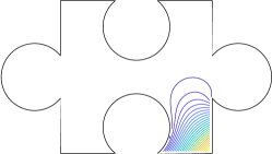
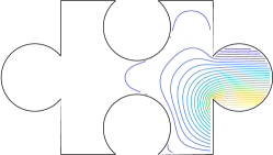
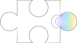
Figure 1. Top Left: The puzzle piece mesh cell considered in Example 4.4 (and Example 4.1). Top Right: The fictitious point $z$ and equilateral triangle used to define $\mathbb{P}_{1}(e)$ for the circular arc of the right tab; this construction was used to provide boundary values in the for the vertex functions $v_{4}$ and $v_{5}$, and the edge function $u_{1}$. Bottom Panel: Contour plots of $v_{3},v_{4},u_{1}\in V_{1}^{\partial K}(K)=V_{1}(K)$, left to right.

As in Example 4.2, we let $v_{j}$ denote a vertex function, i.e. the harmonic function satisfying $v_{j}(z_{i})=\delta_{ij}$ for each of the 12 vertices $z_{i}$, such that, along each edge, the trace of $v_{j}$ is the trace of a linear function. On straight edges, this corresponds to our natural understanding of linear functions of a single variable such as arclength, but we must clarify what we use for linear functions on curved edges. Using the curved edge $e$ (a circular arc) having $z_{4}$ and $z_{5}$ as its endpoints, we introduce a fictitious equilateral triangle that includes a fictitious point $z$, as seen in Figure 1. The three (linear) barycentric coordinates of this triangle are defined in all of $\mathbb{R}^{2}$, and we take their traces on $e$ to define $\mathbb{P}_{1}(e)$. The traces on $e$ of the barycentric coordinates associated with $z_{4}$ and $z_{5}$ provide part of the Dirichlet data for $v_{4}$ and $v_{5}$. Analogous constructions are used for the other three curved edges. This discussion also makes it clear that, in addition to the 12 vertex functions in $V_{1}(K)$, there are four “edge functions” in $V_{1}(K)$, associated with the four curved edges of $\partial K$, which are harmonic and vanish at every vertex, and whose trace on a curved edge is the trace of a linear function on that edge, as described above. We label these edge functions $u_{0},u_{1},u_{2},u_{3}$, where the Dirichlet trace of $u_{0}$ is supported on the curved edge of the bottom blank, that of $u_{1}$ is supported on the curved edge of the right tab, that of $u_{2}$ is supported on the curved edge of the top blank, and that of $u_{3}$ is supported on the curved edge of the left tab. Although we will not need to evaluate any of these functions in (the interior of) $K$ for our integral computations, we provide contour plots of three functions from $V_{1}(K)$ to further clarify our constructions. We note that $\dim V_{1}(K)=\dim\mathbb{P}_{1}^{*}(\partial K)=16$. For all curved edges, we choose the equilateral triangle so that the fictitious point is directed away from the center of $K$. This has the effect that non-zero Dirichlet values of $u_{1}$ and $u_{3}$ (associated with the tabs) are positive, and the non-zero Dirichlet values of $u_{0}$ and $u_{2}$ (associated with the blanks) are negative; so $u_{1},u_{3}>0$ and $u_{0},u_{2}<0$ in the interior of $K$.

On a straight edge $e$, $\dim\mathbb{P}_{2}(e)=3$, but on a circular edge $e$, $\dim\mathbb{P}_{2}(e)=5$ (cf. [2, Proposition 2.1]). From this, it follows that $\dim\mathbb{P}_{2}^{*}(\partial K)=32$. We can augment our basis of $\mathbb{P}_{1}^{*}(\partial K)$ with 16 additional functions, whose traces on an edge $e$ are traces of quadratic functions $e$, to obtain a basis of $\mathbb{P}_{2}^{*}(\partial K)$. These, in turn yield functions in $V_{2}^{\partial K}(K)$ by harmonic extension, as before. We will only consider the following 12, which are sufficient for our quadrature illustrations: $w_{j}\in V_{2}^{\partial K}(K)$ is the harmonic function satisfying $w_{j}=v_{j}v_{j+1}$ on $\partial K$.

In Table 6, we use our quadrature method to compute the integrals in (3) for several representative choices of $v,w$ taken from the hierarchical basis of $V_{2}(K)$ we have constructed above. Apart from the known value $\int_{K}\nabla v\cdot\nabla w\,dx=0$ for $v\in V_{2}^{\partial K}(K)$ and $w\in V_{2}^{K}(K)$, exact values are not available, so we report the computed values to enough digits to observe convergence patterns. Comparing the values computed for $n=32$ and $n=64$, we observe that the $L^{2}$ inner products typically differ on the order $10^{-8}$, while the $H^{1}$ semi-inner products typically differ by about $10^{-6}$. These observations are consistent with the absolute errors observed in Example 4.3, which similarly featured a domain with non-convex corners, giving rise to singular functions having unbounded gradients near such corners.

Table 6. Computed values of the $L^{2}$ inner product $\int_{K}vw~{}dx$ and the $H^{1}$ semi-inner product $\int_{K}\nabla v\cdot\nabla w~{}dx$ on the Puzzle Piece, as described in Example 4.4. Following the notation in that example, $v_{j}$ denotes the linear vertex functions, $u_{j}$ denotes the linear edge functions, $w_{j}$ denotes the quadratic edge functions, and $\tilde{w}$ denotes the bubble function.

$v$	$w$	$n$	$L^{2}$ computed	$H^{1}$ computed
$v_{0}$	$v_{0}$	4	1.36722100e-02	7.26172648e-01
		8	1.39162733e-02	7.24767603e-01
		16	1.39041636e-02	7.25599803e-01
		32	1.39043324e-02	7.25576824e-01
		64	1.39043346e-02	7.25576695e-01
$v_{0}$	$v_{1}$	4	1.05818498e-02	-5.48518347e-01
		8	9.16414178e-03	-5.66262962e-01
		16	9.17500217e-03	-5.66136764e-01
		32	9.17618664e-03	-5.66201634e-01
		64	9.17618833e-03	-5.66201663e-01
$v_{0}$	$w_{0}$	4	1.81794593e-03	1.28954443e-01
		8	2.01809269e-03	1.24305855e-01
		16	2.01072985e-03	1.24548106e-01
		32	2.01040843e-03	1.24569497e-01
		64	2.01040886e-03	1.24569472e-01
$v_{1}$	$u_{0}$	4	-8.30808861e-03	-8.59205540e-01
		8	-1.08862664e-02	-1.10211908e+00
		16	-1.07049968e-02	-1.09593380e+00
		32	-1.07051888e-02	-1.09590692e+00
		64	-1.07051900e-02	-1.09590691e+00
$u_{0}$	$u_{0}$	4	1.00392937e-01	6.09807959e+00
		8	1.27777179e-01	7.38466056e+00
		16	1.27439875e-01	7.37314091e+00
		32	1.27460415e-01	7.37307150e+00
		64	1.27460423e-01	7.37307096e+00
$u_{0}$	$u_{4}$	4	-5.39752362e-03	1.30869343e-01
		8	-3.92970591e-03	9.61489506e-02
		16	-3.91163646e-03	9.47669194e-02
		32	-3.92266750e-03	9.50284316e-02
		64	-3.92268446e-03	9.50288434e-02
$\tilde{w}$	$\tilde{w}$	4	1.98651110e-04	1.19301041e-02
		8	1.36096130e-04	9.87645211e-03
		16	1.36275143e-04	9.85192757e-03
		32	1.36415508e-04	9.85631214e-03
		64	1.36415772e-04	9.85632205e-03
$v_{0}$	$\tilde{w}$	4	4.06902400e-04	0
		8	2.35312339e-04	0
		16	2.35317337e-04	0
		32	2.35506723e-04	0
		64	2.35507154e-04	0
$u_{3}$	$\tilde{w}$	4	-5.49240260e-04	0
		8	-1.07144403e-03	0
		16	-1.06639357e-03	0
		32	-1.06754253e-03	0
		64	-1.06754457e-03	0

5. Additional Details

In [31] we discuss, in detail, integral equation techniques to compute interior function values and derivatives, as well as the normal derivative, of harmonic functions with prescribed Dirichlet data. That paper also involves a detailed discussion of the so-called Kress quadrature that underlies much of the practical computations. Readers interested in that level of detail for these aspects of our present work are referred to that paper. Here, we merely outline key components to make this paper a bit more self-contained, and to explain the parameters $n$ and $\sigma$ used for the experiments in the Section 4.

A fundamental step in the techniques in [31] is the computation of a harmonic conjugate $\hat{\phi}$ of a harmonic function $\phi$ that is given implicitly by its Dirichlet data. The associated boundary value problem for $\hat{\phi}$ is given in (8), and we emphasize its general form as a Neumann problem,

$$\Delta\hat{\phi}=0\mbox{ in }K\quad,\quad\frac{\partial\hat{\phi}}{\partial\mathbf{n}}=g\mbox{ on }\partial K\quad,\quad\int_{\partial K}\hat{\phi}\,ds=0~{}.$$

as such problems also arise in the construction described in Proposition 2.2. Here, the Neumann data $g$ is specified by the user. We provide the associated integral equation employed in our work, whose solution yields a Neumann-to-Dirichlet map $g\to\hat{\phi}|_{\partial K}$. We only present the equation in the case that $\partial K$ has a single corner $z$. The case of multiple corners is dealt with analogously, and further details are provided in [31]. The associated integral equation is

(18) $$|\partial K|\hat{\phi}(z)+\frac{\hat{\phi}(x)-\hat{\phi}(z)}{2}+\int_{\partial K}\left(\frac{\partial G(x,y)}{\partial\mathbf{n}(y)}+1\right)(\hat{\phi}(y)-\hat{\phi}(z))\,ds(y)=\int_{\partial K}G(x,y)g(y)\,ds(y)~{},$$

where $G(x,y)=-(2\pi)^{-1}\ln|x-y|$ is the fundamental solution for the Laplacian in 2D. This integral equation is discretized by a Nyström method, which is a quadrature based method in which the integrals from (18) in the variable $y$ are replaced by a quadrature that is suitable for these integrands regardless of the choice of $x\in\partial\Omega$, resulting in a “semi-discrete” equation. The semi-discrete equation is then sampled at the quadrature points to obtain a fully discrete (and well-conditioned) square linear system. We solve this system using GMRES. In the case that $\hat{\phi}$ is a harmonic conjugate of the harmonic function $\phi$ having Dirichlet data $f$, a Dirichlet-to-Neumann map $f\mapsto\partial\phi/\partial\mathbf{n}$ is obtained by taking the tangential derivative of $\hat{\phi}$, $\partial\phi/\partial\mathbf{n}=\partial\hat{\phi}/\partial\mathbf{t}$. In our computations, an FFT is used to efficiently approximate $\partial\hat{\phi}/\partial\mathbf{t}$ at quadrature points from the approximation of $\hat{\phi}$ at these points that was obtained by solving the Nyström linear system.

The fundamental quadrature used in our discretization is due to Kress [29], and we briefly describe it here to explain the parameters $n$ and $\sigma$ used for the experiments. Suppose that a function $F$ is continuous on $[a,b]$. For any suitable change-of-variable $t=\lambda(\tau)$, $\lambda:[a,b]\to[a,b]$, we have $\int_{a}^{b}F(t)\,dt=\int_{a}^{b}F(\lambda(\tau))\lambda^{\prime}(\tau)\,d\tau$. A clever choice of $\lambda$ ensures that the new integrand, $F(\lambda(\tau))\lambda^{\prime}(\tau)$, vanishes at the endpoints $a$ and $b$, together with some of its derivatives. It is well-known that the trapezoid rule converges rapidly for such integrands, with the rate of convergence depending on the order at which $F(\lambda(\tau))\lambda^{\prime}(\tau)$ vanishes at these endpoints. Kress quadrature is obtained by using the trapezoid rule after the following sigmoidal change-of-variable, which is determined by single integer parameter $\sigma\geq 2$,

(19) $$\lambda(\tau)=(b-a)\frac{[c(\tau)]^{\sigma}}{[c(\tau)]^{\sigma}+[1-c(\tau)]^{\sigma}}+a\quad,\quad c(\tau)=\left(\frac{1}{2}-\frac{1}{\sigma}\right)\theta^{2}+\frac{\theta}{\sigma}+\frac{1}{2}~{},$$

where $\theta=(2\tau-a-b)/(b-a)$. A key property of this change-of-variable is that $\lambda^{\prime}(\tau)$ has roots of order $\sigma-1$ at $\tau=a$ and $\tau=b$. Letting $h=(b-a)/m$ and $\tau_{k}=a+kh$, for $0\leq k\leq m$, the corresponding quadrature is

(20) $$\int_{a}^{b}F(t)\,dt\approx\sideset{}{{}^{\prime\prime}}{\sum}_{k=0}^{m}F(t_{k})w_{k}=\sum_{k=1}^{m-1}F(t_{k})w_{k}\quad,\quad t_{k}=\lambda(\tau_{k})\quad,\quad w_{k}=h\lambda^{\prime}(\tau_{k})~{}.$$

The double-prime notation in the first sum above indicates that its initial and final terms are halved. Since $w_{0}=w_{m}=0$, these terms can be dropped. Kress provides an analysis of this quadrature based on the Euler-Maclaurin formula in [29], and we provide a complementary analysis based on Fourier series in [31]. Depending on whether both, one or neither of the endpoints are counted, (20) involves between $m-1$ and $m+1$ quadrature points. It is convenient in our applications to consider it as an $m$-point quadrature by including only one of the endpoints, so that $m$ points are “assigned” to each edge of $\partial K$ via a parameterization of the boundary, and each vertex of $\partial K$ is counted only once. It is also convenient in our implementation to take $m=2n$. This choice applies both to the quadrature used for the Nyström linear system, which yields our discrete Dirichlet-to-Neumann map, and for the final boundary quadratures that employ this data to compute the target integrals (3) as described in the introductory paragraph of Section 4. When the integer parameter $n$ is used in Section 4, this is what it indicates.

We include an extension of Table 1 as a ready reference that may be used for higher degree polynomials. This is given in Table 7 and covers multiindices $\alpha$ for which $7\leq|\alpha|\leq 10$. We also make a brief note on computing the products of polynomials in our context. Given $p,q\in\mathbb{P}_{m}(\mathbb{R}^{2})$, with

$$p(x)=\sum_{|\alpha|\leq m}c_{\alpha}(x-z)^{\alpha}~{},\quad q(x)=\sum_{|\beta|\leq m}d_{\beta}(x-z)^{\beta}~{},$$

the product $pq\in\mathbb{P}_{2m}(\mathbb{R}^{2})$ may be written as

$$(pq)(x)=\sum_{|\gamma|\leq 2m}\tilde{c}_{\gamma}(x-z)^{\gamma}~{},$$

where the coefficients are given by

$$\tilde{c}_{\gamma}=\sum_{|\alpha|+|\beta|=|\gamma|}c_{\alpha}d_{\beta}~{}.$$

In the case where $p,q$ are sparse, i.e. the majority of their coefficients are zero, as is the case for our experiments, we execute a double loop over the nonzero coefficients of $p$ and $q$, and for each pair $(\alpha,\beta)$, we determine the integer $n$ corresponding to the multi-index $\alpha+\beta$, according to the bijection described in (5). We then increment the coefficient $\tilde{c}_{\gamma}$, with $\gamma$ corresponding to $n$, with $\tilde{c}_{\gamma}\leftarrow\tilde{c}_{\gamma}+c_{\alpha}d_{\beta}$.

Table 7. An enumeration of multiindices for $7\leq|\alpha|\leq 10$, together with the indices and values of the non-zero coefficients of $P_{\alpha}$ from Proposition 2.1.

$k$	$\alpha$	$P_{\alpha}$ indices	$P_{\alpha}$ coefficients
28	$(7,0)$	$(45,47,49,51,53)$	$(85,12,-42,28,-3)/6144$
29	$(6,1)$	$(46,48,50,52,54)$	$(247,84,-126,36,-1)/14336$
30	$(5,2)$	$(45,47,49,51,53)$	$(-73,2628,1554,-1036,111)/129024$
31	$(4,3)$	$(46,48,50,52,54)$	$(-489,4564,3906,-1116,31)/215040$
32	$(3,4)$	$(45,47,49,51,53)$	$(31,-1116,3906,4564,-489)/215040$
33	$(2,5)$	$(46,48,50,52,54)$	$(111,-1036,1554,2628,-73)/129024$
34	$(1,6)$	$(45,47,49,51,53)$	$(-1,36,-126,84,247)/14336$
35	$(0,7)$	$(46,48,50,52,54)$	$(-3,28,-42,12,85)/6144$
36	$(8,0)$	$(55,57,59,61,63,65)$	$(511,45,-210,210,-45,1)/46080$
37	$(7,1)$	$(56,58,60,62,64)$	$(251,60,-126,60,-5)/18432$
38	$(6,2)$	$(55,57,59,61,63,65)$	$(-233,10485,4830,-4830,1035,-23)/645120$
39	$(5,3)$	$(56,58,60,62,64)$	$(-191,2292,1638,-780,65)/129024$
40	$(4,4)$	$(55,57,59,61,63,65)$	$(1,-45,210,210,-45,1)/12600$
41	$(3,5)$	$(56,58,60,62,64)$	$(65,-780,1638,2292,-191)/129024$
42	$(2,6)$	$(55,57,59,61,63,65)$	$(-23,1035,-4830,4830,10485,-233)/645120$
43	$(1,7)$	$(56,58,60,62,64)$	$(-5,60,-126,60,251)/18432$
44	$(0,8)$	$(55,57,59,61,63,65)$	$(1,-45,210,-210,45,511)/46080$
45	$(9,0)$	$(66,68,70,72,74,76)$	$(93,5,-30,42,-15,1)/10240$
46	$(8,1)$	$(67,69,71,73,75,77)$	$(1013,165,-462,330,-55,1)/92160$
47	$(7,2)$	$(66,68,70,72,74,76)$	$(-11,605,210,-294,105,-7)/46080$
48	$(6,3)$	$(67,69,71,73,75,77)$	$(-53,795,462,-330,55,-1)/53760$
49	$(5,4)$	$(66,68,70,72,74,76)$	$(29,-1595,9570,8106,-2895,193)/645120$
50	$(4,5)$	$(67,69,71,73,75,77)$	$(193,-2895,8106,9570,-1595,29)/645120$
51	$(3,6)$	$(66,68,70,72,74,76)$	$(-1,55,-330,462,795,-53)/53760$
52	$(2,7)$	$(67,69,71,73,75,77)$	$(-7,105,-294,210,605,-11)/46080$
53	$(1,8)$	$(66,68,70,72,74,76)$	$(1,-55,330,-462,165,1013)/92160$
54	$(0,9)$	$(67,69,71,73,75,77)$	$(1,-15,42,-30,5,93)/10240$
55	$(10,0)$	$(78,80,82,84,86,88,90)$	$(2047,66,-495,924,-495,66,-1)/270336$
56	$(9,1)$	$(79,81,83,85,87,89)$	$(509,55,-198,198,-55,3)/56320$
57	$(8,2)$	$(78,80,82,84,86,88,90)$	$(-1981,130746,33165,-61908,33165,-4422,67)/12165120$
58	$(7,3)$	$(79,81,83,85,87,89)$	$(-681,12485,5742,-5742,1595,-87)/1013760$
59	$(6,4)$	$(78,80,82,84,86,88,90)$	$(743,-49038,367785,259644,-139095,18546,-281)/28385280$
60	$(5,5)$	$(79,81,83,85,87,89)$	$(3,-55,198,198,-55,3)/16632$
61	$(4,6)$	$(78,80,82,84,86,88,90)$	$(-281,18546,-139095,259644,367785,-49038,743)/28385280$
62	$(3,7)$	$(79,81,83,85,87,89)$	$(-87,1595,-5742,5742,12485,-681)/1013760$
63	$(2,8)$	$(78,80,82,84,86,88,90)$	$(67,-4422,33165,-61908,33165,130746,-1981)/12165120$
64	$(1,9)$	$(79,81,83,85,87,89)$	$(3,-55,198,-198,55,509)/56320$
65	$(0,10)$	$(78,80,82,84,86,88,90)$	$(-1,66,-495,924,-495,66,2047)/270336$

All of the numerical experiments in this paper were implemented in Matlab. Those interested in obtaining a copy of our code may do so at the GitHub repository found at

https://github.com/samreynoldsmath/HigherOrderCurvedElementQuadrature

6. Concluding Remarks

We have described an approach for integrating products of functions and their gradients over curvilinear polygons, when the functions are given implicitly in terms of Poisson problems involving polynomial data. The efficient and accurate evaluation of such integrals is instrumental in the formation of linear systems associated with finite element methods such as Trefftz-FEM and VEM, which employ non-standard meshes. In our approach, integrals on curvilinear polygonal cells are reduced to integrals along their boundaries, using constructions that yield a function whose Laplacian is a given polynomial or harmonic function, together with integration by parts. The data for quadrature approximations of these boundary integrals is obtained using Dirichlet-to-Neumann and Neumann-to-Dirichlet maps that are computed using techniques based on second-kind integral equations. Numerical examples demonstrate rapid convergence and high accuracy of these quadratures.

References

- [1] B. Ahmad, A. Alsaedi, F. Brezzi, L. D. Marini, and A. Russo. Equivalent projectors for virtual element methods. Comput. Math. Appl., 66(3):376–391, 2013.
- [2] A. Anand, J. S. Ovall, S. E. Reynolds, and S. Weißer. Trefftz Finite Elements on Curvilinear Polygons. SIAM J. Sci. Comput., 42(2):A1289–A1316, 2020.
- [3] A. Anand, J. S. Ovall, and S. Weißer. A Nyström-based finite element method on polygonal elements. Comput. Math. Appl., 75(11):3971–3986, 2018.
- [4] P. F. Antonietti, L. Beirão da Veiga, D. Mora, and M. Verani. A stream virtual element formulation of the Stokes problem on polygonal meshes. SIAM J. Numer. Anal., 52(1):386–404, 2014.
- [5] P. F. Antonietti, S. Berrone, M. Verani, and S. Weißer. The virtual element method on anisotropic polygonal discretizations. In Numerical mathematics and advanced applications—ENUMATH 2017, volume 126 of Lect. Notes Comput. Sci. Eng., pages 725–733. Springer, Cham, 2019.
- [6] P. F. Antonietti, M. Bruggi, S. Scacchi, and M. Verani. On the virtual element method for topology optimization on polygonal meshes: a numerical study. Comput. Math. Appl., 74(5):1091–1109, 2017.
- [7] P. F. Antonietti, P. Houston, and G. Pennesi. Fast numerical integration on polytopic meshes with applications to discontinuous Galerkin finite element methods. J. Sci. Comput., 77(3):1339–1370, 2018.
- [8] E. Artioli, A. Sommariva, and M. Vianello. Algebraic cubature on polygonal elements with a circular edge. Comput. Math. Appl., 79(7):2057–2066, 2020.
- [9] L. Beirão da Veiga, F. Brezzi, L. D. Marini, and A. Russo. Polynomial preserving virtual elements with curved edges. Math. Models Methods Appl. Sci., 30(8):1555–1590, 2020.
- [10] L. Beirão da Veiga, A. Russo, and G. Vacca. The virtual element method with curved edges. ESAIM Math. Model. Numer. Anal., 53(2):375–404, 2019.
- [11] L. Beirão da Veiga, F. Brezzi, A. Cangiani, G. Manzini, L. D. Marini, and A. Russo. Basic principles of virtual element methods. Math. Models Methods Appl. Sci., 23(1):199–214, 2013.
- [12] L. Beirão da Veiga, F. Brezzi, L. D. Marini, and A. Russo. The hitchhiker’s guide to the virtual element method. Math. Models Methods Appl. Sci., 24(8):1541–1573, 2014.
- [13] L. Beirão da Veiga, A. Chernov, L. Mascotto, and A. Russo. Basic principles of virtual elements on quasiuniform meshes. Math. Models Methods Appl. Sci., 26(8):1567–1598, 2016.
- [14] L. Beirão da Veiga and G. Manzini. A virtual element method with arbitrary regularity. IMA J. Numer. Anal., 34(2):759–781, 2014.
- [15] M. F. Benedetto, S. Berrone, A. Borio, S. Pieraccini, and S. Scialò. Order preserving SUPG stabilization for the virtual element formulation of advection-diffusion problems. Comput. Methods Appl. Mech. Engrg., 311:18–40, 2016.
- [16] F. Brezzi and L. D. Marini. Virtual element and discontinuous Galerkin methods. In Recent developments in discontinuous Galerkin finite element methods for partial differential equations, volume 157 of IMA Vol. Math. Appl., pages 209–221. Springer, Cham, 2014.
- [17] O. P. Bruno, J. S. Ovall, and C. Turc. A high-order integral algorithm for highly singular PDE solutions in Lipschitz domains. Computing, 84(3-4):149–181, 2009.
- [18] D. Copeland, U. Langer, and D. Pusch. From the boundary element domain decomposition methods to local Trefftz finite element methods on polyhedral meshes. In Domain decomposition methods in science and engineering XVIII, volume 70 of Lect. Notes Comput. Sci. Eng., pages 315–322. Springer, Berlin, 2009.
- [19] M. S. Floater. Generalized barycentric coordinates and applications. Acta Numer., 24:161–214, 2015.
- [20] A. L. Gain, C. Talischi, and G. H. Paulino. On the Virtual Element Method for three-dimensional linear elasticity problems on arbitrary polyhedral meshes. Comput. Methods Appl. Mech. Engrg., 282:132–160, 2014.
- [21] I. S. Gradshteyn and I. M. Ryzhik. Table of integrals, series, and products. Elsevier/Academic Press, Amsterdam, seventh edition, 2007. Translated from the Russian, Translation edited and with a preface by Alan Jeffrey and Daniel Zwillinger, With one CD-ROM (Windows, Macintosh and UNIX).
- [22] P. Grisvard. Elliptic problems in nonsmooth domains, volume 24 of Monographs and Studies in Mathematics. Pitman (Advanced Publishing Program), Boston, MA, 1985.
- [23] P. Grisvard. Singularities in boundary value problems, volume 22 of Recherches en Mathématiques Appliquées [Research in Applied Mathematics]. Masson, Paris, 1992.
- [24] C. Hofreither. error estimates for a nonstandard finite element method on polyhedral meshes. J. Numer. Math., 19(1):27–39, 2011.
- [25] C. Hofreither, U. Langer, and C. Pechstein. Analysis of a non-standard finite element method based on boundary integral operators. Electron. Trans. Numer. Anal., 37:413–436, 2010.
- [26] C. Hofreither, U. Langer, and S. Weißer. Convection-adapted BEM-based FEM. ZAMM Z. Angew. Math. Mech., 96(12):1467–1481, 2016.
- [27] K. Hormann and N. Sukumar, editors. Generalized barycentric coordinates in computer graphics and computational mechanics. CRC Press, Boca Raton, FL, 2018.
- [28] V. V. Karachik and N. A. Antropova. On the solution of a nonhomogeneous polyharmonic equation and the nonhomogeneous Helmholtz equation. Differ. Uravn., 46(3):384–395, 2010.
- [29] R. Kress. A Nyström method for boundary integral equations in domains with corners. Numer. Math., 58(2):145–161, 1990.
- [30] S. Natarajan, S. Bordas, and D. R. Mahapatra. Numerical integration over arbitrary polygonal domains based on Schwarz-Christoffel conformal mapping. Internat. J. Numer. Methods Engrg., 80(1):103–134, 2009.
- [31] J. S. Ovall and S. E. Reynolds. A high-order method for evaluating derivatives of harmonic functions in planar domains. SIAM J. Sci. Comput., 40(3):A1915–A1935, 2018.
- [32] S. Rjasanow and S. Weißer. Higher order BEM-based FEM on polygonal meshes. SIAM J. Numer. Anal., 50(5):2357–2378, 2012.
- [33] S. Rjasanow and S. Weißer. FEM with Trefftz trial functions on polyhedral elements. J. Comput. Appl. Math., 263:202–217, 2014.
- [34] D. Seibel and S. Weißer. Recovery-based error estimators for the VEM and BEM-based FEM. Comput. Math. Appl., 80(9):2073–2089, 2020.
- [35] A. Sommariva and M. Vianello. Product Gauss cubature over polygons based on Green’s integration formula. BIT, 47(2):441–453, 2007.
- [36] Y. Sudhakar, J. M. de Almeida, and W. A. Wall. An accurate, robust, and easy-to-implement method for integration over arbitrary polyhedra: Application to embedded interface methods. J. Comput. Phys., 273:393 – 415, 2014.
- [37] Y. Sudhakar, A. Sommariva, M. Vianello, and W. A. Wall. On the use of compressed polyhedral quadrature formulas in embedded interface methods. SIAM J. Sci. Comput., 39(3):B571–B587, 2017.
- [38] C. Talischi and G. H. Paulino. Addressing integration error for polygonal finite elements through polynomial projections: a patch test connection. Math. Models Methods Appl. Sci., 24(8):1701–1727, 2014.
- [39] S. Weißer. Residual error estimate for bem-based fem on polygonal meshes. Numer. Math., 118:765–788, 2011. 10.1007/s00211-011-0371-6.
- [40] S. Weißer. Arbitrary order Trefftz-like basis functions on polygonal meshes and realization in BEM-based FEM. Comput. Math. Appl., 67(7):1390–1406, 2014.
- [41] S. Weißer. Residual based error estimate and quasi-interpolation on polygonal meshes for high order BEM-based FEM. Comput. Math. Appl., 73(2):187–202, 2017.
- [42] S. Weißer. Anisotropic polygonal and polyhedral discretizations in finite element analysis. ESAIM Math. Model. Numer. Anal., 53(2):475–501, 2019.
- [43] S. Weißer. BEM-based Finite Element Approaches on Polytopal Meshes, volume 130 of Lecture Notes in Computational Science and Engineering. Springer International Publishing, 1 edition, 2019.
- [44] S. Weißer and T. Wick. The dual-weighted residual estimator realized on polygonal meshes. Comput. Methods Appl. Math., 18(4):753–776, 2018.
- [45] N. M. Wigley. Asymptotic expansions at a corner of solutions of mixed boundary value problems. J. Math. Mech., 13:549–576, 1964.
- [46] N. M. Wigley. On a method to subtract off a singularity at a corner for the Dirichlet or Neumann problem. Math. Comp., 23:395–401, 1969.