A corrected transport-velocity formulation for fluid and structural mechanics with SPH

Abstract

Particle shifting techniques (PST) have been used to improve the accuracy of the Smoothed Particle Hydrodynamics (SPH) method. Shifting ensures that the particles are distributed homogeneously in space. This may be performed by moving the particles using a transport velocity. In this paper, we propose an extension to the class of Transport Velocity Formulation (TVF) methods. We derive the equations in a consistent manner and show that there are additional terms that significantly improve the accuracy of the method. In particular, we apply this to the Entropically Damped Artificial Compressibility SPH method. We identify the free-surface particles and their normals using a simple approach and thereby adapt the method for free-surface problems. We show how the new method can be applied to the problem of elastic dynamics. We consider a suite of benchmark problems involving both fluid and solid mechanics to demonstrate the accuracy and applicability of the method. The implementation is open source, and the manuscript is fully reproducible.

1 Introduction

The smoothed particle hydrodynamics (SPH) method has been widely applied since it was originally proposed to simulate hydrodynamic problems in astrophysics independently by Lucy [1], and Gingold and Monaghan [2]. The method has been applied in particular to both compressible [3], incompressible fluid flows [4, 5] as well as elastic dynamics problems [6, 7] in addition to a variety of other problems[8, 9, 10, 11].

The method is meshless and Lagrangian, and therefore particles move with the local velocity. This motion can introduce disorder in the particles and thereby significantly reduce the accuracy of the method. Xu et al. [12] proposed an approach to shift the particles so as to obtain a uniform distribution of particles. This significantly improves accuracy and the method is referred to as the Particle Shifting Technique (PST). Many different kinds of PST methods are available in the literature [13, 14, 15, 16]. An alternative approach that ensures particle homogenization for incompressible fluid flow was proposed as the Transport Velocity Formulation (TVF) [17]. The method introduced an additional stress term to account for the motion introduced by the particle shifting. The TVF produces very accurate results but only works for internal flows. Zhang et al. [18] proposed the Generalized Transport Velocity Formulation (GTVF) thereby allowing the TVF to be used for free-surface problems as well as elastic dynamics problems. This allows for a unified treatment of both fluids and solids. Similarly, Oger et al. [19] introduce ideas from a consistent ALE formulation for improving the accuracy of SPH. They employ a Riemann-based formulation to solve fluid mechanics problems and introduce particle shifting to obtain highly accurate simulations for internal and free-surface problems may also be handled. The PST has also been employed in the context of the $\delta$-SPH schemes[20].

The Entropically Damped Artificial Compressibility SPH scheme (EDAC-SPH) [21] introduces an evolution equation for the pressure and significantly reduces the noise in the pressure since it features a pressure diffusion term. The approach has a thermodynamic justification [22] and produces very accurate results [21]. The EDAC-SPH method uses the TVF formulation for internal flows and for free-surface flows it does not employ any form of particle shifting.

Recently, Antuono et al. [23] carefully combine the ALE-SPH method of Oger et al. [19] and the consistent $\delta$-SPH formulation of Sun et al. [20] to improve the accuracy of the $\delta$-SPH method. They show the importance of the additional terms to the accuracy.

With the notable exception of the GTVF scheme [18], most other applications of the PST have been in the context of fluid mechanics. The GTVF method provides a unified approach to solve both weakly-compressible fluids as well as solids. However, the method suffers from a few issues. In order to work for free-surface problems the method relies on using a different background pressure for each particle and introduces a few numerical corrections to work around issues. For example, the smoothing length of the homogenization force is different from that used by the other equations and this parameter is somewhat ad-hoc. For solid mechanics problems the method uses the transport velocity of the particle rather than the true velocity in order to compute the strain and rotation tensor. In addition there are some terms in the governing equations that are ignored which play a major role. We also note that the method is not robust to a change in the particle homogenization force.

In this work we propose a scheme which we called Corrected Transport Velocity Formulation (CTVF) that is inspired by the various recent developments but is consistent and which works for both solid mechanics and fluid mechanics problems. We derive the transport velocity equations afresh and note that there are some important terms that are ignored in earlier approaches using TVF. These terms are significant and improve the accuracy of the method. Similar to [19, 20], we detect the free surface particles and compute their normals using a simpler and computationally efficient approach which does not require the computation of eigenvalues. This allows the method to work with free-surfaces without the introduction of numerical parameters or a variable background pressure. We employ the EDAC formulation and show that there are additional correction terms in the EDAC scheme that should be introduced to improve the accuracy of the method. Furthermore, we show how the EDAC scheme can be used in the context of solid mechanics problems. We make use of the particle velocity rather than the transport velocity to compute the velocity gradient, strain, and rotation rate tensors. Our method can be used with any PST and we consider the method of Sun et al. [20] as well as the iterative PST of Huang et al. [15]. The method is also robust to the choice of the smoothing kernel. The resulting method works for both weakly-compressible fluids as well as solids. The new method may be thought of as an improved extension of the EDAC-SPH method that can be used for free-surface problems as well as solid mechanics problems.

The method is implemented using the PySPH framework [24, 25]. The source code for all the problems demonstrated in this manuscript is made available at https://gitlab.com/pypr/ctvf. Every result produced in the manuscript is fully automated using the automan package [26].

We next discuss the formulation for fluid mechanics as well as solid mechanics along with the use of particle shifting. The consistent correction terms are derived. We then consider a suite of benchmark problems for both fluids and solids and compare our results with those of other methods where applicable.

2 Governing equations

For elastic dynamics we use the same equations as in [7, 18] which we summarize below. The governing equations of motion involve the conservation of mass, which in Lagrangian form is,

$$\frac{d\rho}{dt}=-\rho\;\frac{\partial u_{i}}{\partial x_{i}},$$ (1)

and conservation of linear momentum,

$$\frac{du_{i}}{dt}=\frac{1}{\rho}\;\frac{\partial\sigma_{ij}}{\partial x_{j}}+g_{i},$$ (2)

where $\rho$ is the density, $u_{i}$ is the $i$^th component of the velocity field, $x_{j}$ is the $j$^th component of the position vector, $g_{i}$ is the component of body force per unit mass and $\sigma_{ij}$ is stress tensor.

The stress tensor is split into isotropic and deviatoric parts,

$$\sigma_{ij}=-p\;\delta_{ij}+\sigma^{\prime}_{ij},$$ (3)

where $p$ is the pressure, $\delta_{ij}$ is the Kronecker delta function, and $\sigma^{\prime}_{ij}$ is the deviatoric stress.

The Jaumann’s formulation for Hooke’s stress provides us with the rate of change of deviatoric stress,

$$\frac{d\sigma^{\prime}_{ij}}{dt}=2G(\dot{\epsilon}_{ij}-\frac{1}{3}\dot{\epsilon}_{kk}\delta_{ij})+\sigma^{{}^{\prime}}_{ik}\Omega_{jk}+\Omega_{ik}\sigma^{{}^{\prime}}_{kj},$$ (4)

where $G$ is the shear modulus, $\dot{\epsilon}_{ij}$ is the strain rate tensor,

$$\dot{\epsilon}_{ij}=\frac{1}{2}\bigg{(}\frac{\partial u_{i}}{\partial x_{j}}+\frac{\partial u_{j}}{\partial x_{i}}\bigg{)},$$ (5)

and $\Omega_{ij}$ is the rotation tensor,

$$\Omega_{ij}=\frac{1}{2}\bigg{(}\frac{\partial u_{i}}{\partial x_{j}}-\frac{\partial u_{j}}{\partial x_{i}}\bigg{)}.$$ (6)

For a weakly-compressible or incompressible fluid, a viscous force is added:

$$\sigma_{ij}=-p\delta_{ij}+2\eta\frac{\partial u_{i}}{\partial x_{j}}$$ (7)

where $\eta$ is the kinematic viscosity of the fluid.

In both fluid and solid modelling the pressure is computed using an isothermal equation of state, given as,

$$p=K\bigg{(}\frac{\rho}{\rho_{0}}-1\bigg{)},$$ (8)

where $K=\rho_{0}c_{0}^{2}$ is the bulk modulus. Here, the constants $c_{0}$ and $\rho_{0}$ are the reference speed of sound and density, respectively. For solids, $c_{0}$ is computed as $\sqrt{\frac{E}{3(1-2\nu)\rho_{0}}}$, $\nu$ is the Poisson ratio.

3 Numerical method

Following the TVF [17] and similar formulations [19], we move the particles with a transport velocity, $\tilde{\mathbf{u}}$. The material derivative in this case is written as,

$$\frac{\tilde{d}}{dt}=\frac{\partial}{\partial t}+\tilde{u}_{j}\frac{\partial}{\partial x_{j}}.$$ (9)

We therefore recast the governing equations to incorporate the transport velocity starting with the conservation of mass, equation (1),

$$\frac{\tilde{d}\rho}{dt}=-\rho\frac{\partial u_{j}}{\partial x_{j}}+(\tilde{u}_{j}-u_{j})\frac{\partial\rho}{\partial x_{j}}.$$ (10)

Since,

$$(\tilde{u}_{j}-u_{j})\frac{\partial\rho}{\partial x_{j}}=\frac{\partial(\rho(\tilde{u}_{j}-u_{j}))}{\partial x_{j}}-\rho\frac{\partial(\tilde{u}_{j}-u_{j})}{\partial x_{j}},$$ (11)

we write equation (10), as

$$\frac{\tilde{d}\rho}{dt}=-\rho\frac{\partial\tilde{u}_{j}}{\partial x_{j}}+\frac{\partial(\rho(\tilde{u}_{j}-u_{j}))}{\partial x_{j}}.$$ (12)

By combining the continuity equation (1) and momentum equation (2) one can obtain the conservative form of the momentum equation as,

$$\frac{\partial(\rho u_{i})}{\partial t}+\frac{\partial}{\partial x_{j}}(\rho u_{i}u_{j}) =\rho g_{i}+\frac{\partial\sigma_{ij}}{\partial x_{j}}$$ (13)

$$=\text{RHS}_{i},$$

where $g_{i}$ is the body force acceleration, and $\sigma_{ij}$ the stress tensor. We write the left hand side in terms of a transport derivative as,

$$\frac{\tilde{d}(\rho u_{i})}{dt}+(u_{j}-\tilde{u}_{j})\frac{\partial}{\partial x_{j}}(\rho u_{i})+\rho u_{i}\frac{\partial u_{j}}{\partial x_{j}}=\text{RHS}_{i}.$$ (14)

Similar to eq. 11, we write,

$$(\tilde{u}_{j}-u_{j})\frac{\partial}{\partial x_{j}}(\rho u_{i})=\frac{\partial}{\partial x_{j}}(\rho u_{i}(\tilde{u}_{j}-u_{j}))-\rho u_{i}\frac{\partial}{\partial x_{j}}(\tilde{u}_{j}-u_{j}).$$ (15)

Substituting, this in eq. 14, we have,

$$\frac{\tilde{d}(\rho u_{i})}{dt}=\frac{\partial}{\partial x_{j}}(\rho u_{i}(\tilde{u}_{j}-u_{j}))-\rho u_{i}\frac{\partial}{\partial x_{j}}(\tilde{u}_{j})+\text{RHS}_{i}.$$ (16)

In Adami et al. [17], the second term is neglected but at this stage we do not neglect this term. We simplify this further and write,

$$\rho\frac{\tilde{d}u_{i}}{dt}+u_{i}\frac{\tilde{d}\rho}{dt}=\frac{\partial}{\partial x_{j}}(\rho u_{i}(\tilde{u}_{j}-u_{j}))-\rho u_{i}\frac{\partial}{\partial x_{j}}(\tilde{u}_{j})+\text{RHS}_{i}.$$ (17)

Using, eq. 12, we write

$$\rho\frac{\tilde{d}u_{i}}{dt} =\frac{\partial}{\partial x_{j}}(\rho u_{i}(\tilde{u}_{j}-u_{j}))-u_{i}\frac{\partial}{\partial x_{j}}(\rho(\tilde{u}_{j}-u_{j}))+\text{RHS}_{i}$$ (18)

$$=\rho(\tilde{u}_{j}-u_{j})\frac{\partial u_{i}}{\partial x_{j}}+\text{RHS}_{i}$$

$$=\rho\frac{\partial}{\partial x_{j}}(u_{i}(\tilde{u}_{j}-u_{j}))-\rho u_{i}\frac{\partial}{\partial x_{j}}(\tilde{u}_{j}-u_{j})+\text{RHS}_{i}.$$

We therefore write the momentum equation as,

$$\frac{\tilde{d}u_{i}}{dt}=\frac{\partial}{\partial x_{j}}(u_{i}(\tilde{u}_{j}-u_{j}))-u_{i}\frac{\partial}{\partial x_{j}}(\tilde{u}_{j}-u_{j})+g_{i}+\frac{1}{\rho}\frac{\partial\sigma_{ij}}{\partial x_{j}}.$$ (19)

We note that this equation encompasses both fluid dynamics as well as elastic dynamics by simply changing the way $\sigma_{ij}$ is modeled. The first term on the right-hand-side of eq. 19 is the additional artificial stress term that is included in the TVF [17]. The second term involves the divergence of the transport velocity field. In the case of the TVF, the term includes a background pressure acceleration that is of the form,

$$\bigg{(}\frac{d\mathbf{u}_{a}}{dt}\bigg{)}_{c}=-p^{0}_{a}\sum_{b\in N(a)}\frac{m_{b}}{\rho_{b}^{2}}\nabla W(\mathbf{r}_{ab},\tilde{h}_{ab}),$$ (20)

where $p^{0}_{a}$ is the background pressure for the given particle $a$, $\mathbf{r}_{ab}=\mathbf{r}_{a}-\mathbf{r}_{b}$, $\tilde{h}_{ab}=(h_{a}+h_{b})/2$, and index $b$ refers to the neighbors of particle $a$. The divergence of this term results in the Laplacian of the kernel $W$. For most kernels used in SPH, this term is certainly not zero and therefore this should not be ignored. We investigate the importance of including these terms in section 4. We note that in the case of elastic dynamics that these terms are negligible and do not make a significant difference. This has also been pointed out by Zhang et al. [18].

The Jaumann stress rate is also similarly modified to account for the transport velocity as,

$$\frac{\tilde{d}\sigma^{\prime}_{ij}}{dt}=2G(\dot{\epsilon}_{ij}-\frac{1}{3}\dot{\epsilon}_{kk}\delta_{ij})+\sigma^{{}^{\prime}}_{ik}\Omega_{jk}+\Omega_{ik}\sigma^{{}^{\prime}}_{kj}+\\ \frac{\partial}{\partial x_{k}}\big{(}\sigma^{{}^{\prime}}_{ij}(\tilde{u}_{k}-u_{k})\big{)}-\sigma^{{}^{\prime}}_{ij}\frac{\partial}{\partial x_{k}}(\tilde{u}_{k}-u_{k}).$$ (21)

3.1 The EDAC-SPH method

We apply the EDAC-SPH [21] in order to evolve the pressure accurately and reduce the amount of noise in the pressure field. In the original EDAC-SPH implementation, internal flows were evolved using the TVF whereas for cases with a free-surface the traditional WCSPH was employed. In this work we propose a unified approach by carefully incorporating free-surfaces. The original EDAC-SPH scheme also did not accurately incorporate the transport velocity which we include here. This allows us to use the same scheme for both internal and external flows.

The $\delta$-SPH [27] implementation is in principle similar to the EDAC-SPH method but requires the use of the kernel gradient corrections which involve the solution of a small matrix ($3\times 3$ in 3D), for each particle. The EDAC-SPH method does not require this and is therefore simpler and in principle more efficient. In [21], the EDAC pressure evolution equation was,

$$\frac{dp}{dt}=-\rho c_{s}^{2}\text{div}(\mathbf{u})+\nu_{edac}\nabla^{2}p,$$ (22)

where $\nu_{edac}$ is a viscosity parameter for the smoothing of the pressure and $c_{s}$ is the (artificial) speed of sound. We discuss this term later. However, in the context of the consistent evolution using the transport velocity, we note that the above should be evolved using,

$$\frac{\tilde{d}p}{dt}=(p-\rho c_{s}^{2})\text{div}(\mathbf{u})-p\;\text{div}(\tilde{\mathbf{u}})+\text{div}(p(\tilde{\mathbf{u}}-\mathbf{u}))+\nu_{edac}\nabla^{2}p.$$ (23)

The value of $\nu_{edac}$ is,

$$\nu_{edac}=\frac{\alpha_{\textrm{edac}}hc_{s}}{8},$$ (24)

where $h$ is the smoothing length of the kernel and a value of $\alpha_{\textrm{edac}}=0.5$ is recommended as suggested in [28].

This along with the momentum equation and evolution of volume or density may be employed. A state equation is often used even for elastic dynamics problems, we propose to use the EDAC approach for elastic equations as well as this reduces the amount of artificial viscosity that is needed.

3.2 SPH discretization

In the current work, both fluid and solid modelling uses the same continuity and pressure evolution equation. The SPH discretization of the continuity equation (12) and the pressure evolution equation (23) respectively are,

$$\frac{\tilde{d}\rho_{a}}{dt}=\sum_{b}\;\frac{m_{b}}{\rho_{b}}\;(\rho_{a}\;\tilde{\mathbf{u}}_{ab}\;+\;(\rho\;(\tilde{\mathbf{u}}\;-\;\mathbf{u}))_{ab})\;\cdot\nabla_{a}W_{ab},$$ (25)

$$\frac{\tilde{d}p_{a}}{dt}=\sum_{b}\;\frac{m_{b}}{\rho_{b}}\;\bigg{(}(p_{a}-\rho_{a}c_{s}^{2})\;\mathbf{u}_{ab}\;+\;p_{a}\;\tilde{\mathbf{u}}_{ab}\;-\;(p\;(\tilde{\mathbf{u}}-\mathbf{u}))_{ab}\;+\;\\ 4\;\nu_{edac}\frac{p_{a}-p_{b}}{(\rho_{a}+\rho_{b})(r^{2}_{ab}+0.01h_{ab}^{2})}\mathbf{r}_{ab}\bigg{)}\;\cdot\nabla_{a}W_{ab}.$$ (26)

Similarly, the discretized momentum equation for fluids is written as,

$$\frac{\tilde{d}\mathbf{u}_{a}}{dt}=-\sum_{b}m_{b}\bigg{[}\bigg{(}\frac{p_{a}}{\rho_{a}^{2}}+\frac{p_{b}}{\rho_{b}^{2}}\bigg{)}\mathbf{I}-\bigg{(}\frac{\mathbf{A}_{a}}{\rho_{a}^{2}}+\frac{\mathbf{A}_{b}}{\rho_{b}^{2}}\bigg{)}\bigg{]}\cdot\nabla_{a}W_{ab}\\ +\mathbf{u}_{a}\sum_{b}\frac{m_{b}}{\rho_{b}}\;\tilde{\mathbf{u}}_{ab}\cdot\nabla_{a}W_{ab}+\sum_{b}m_{b}\frac{4\eta\nabla W_{ab}\cdot\mathbf{r}_{ab}}{(\rho_{a}+\rho_{b})(r_{ab}^{2}+0.01h_{ab}^{2})}\mathbf{u}_{ab}+\mathbf{g}_{a},$$ (27)

where $\mathbf{A}_{a}=\rho_{a}\mathbf{u}_{a}\otimes(\mathbf{\tilde{u}}_{a}-\mathbf{u}_{a})$, $\mathbf{I}$ is the identity matrix, $\eta$ is the kinematic viscosity of the fluid and Morris et al. [29] formulation is used to discretize the viscosity term.

We add to the momentum equation an additional artificial viscosity term $\Pi_{ab}$ [3] to maintain the stability of the numerical scheme, given as,

$$\Pi_{ab}=\begin{cases}\frac{-\alpha h_{ab}\bar{c}_{ab}\phi_{ab}}{\bar{\rho}_{ab}}&\mathbf{u}_{ab}\cdot\mathbf{r}_{ab}<0,\\ 0&\mathbf{u}_{ab}\cdot\mathbf{r}_{ab}\geq 0,\end{cases}$$ (28)

where,

$$\phi_{ab}=\frac{\mathbf{u}_{ab}\cdot\mathbf{r}_{ab}}{r^{2}_{ab}+0.01h^{2}_{ab}},$$ (29)

where $\mathbf{r}_{ab}=\mathbf{r}_{a}-\mathbf{r}_{b}$, $\mathbf{u}_{ab}=\mathbf{u}_{a}-\mathbf{u}_{b}$, $h_{ab}=(h_{a}+h_{b})/2$, $\bar{\rho}_{ab}=(\rho_{a}+\rho_{b})/2$, $\bar{c}_{ab}=(c_{a}+c_{b})/2$, and $\alpha$ is the artificial viscosity parameter.

For solid mechanics the momentum equation is written as,

$$\frac{\tilde{d}\mathbf{u}_{a}}{dt}=-\sum_{b}m_{b}\bigg{[}\bigg{(}\frac{p_{a}}{\rho_{a}^{2}}+\frac{p_{b}}{\rho_{b}^{2}}\bigg{)}\mathbf{I}-\bigg{(}\frac{\boldsymbol{\sigma}^{{}^{\prime}}_{a}}{\rho_{a}^{2}}+\frac{\boldsymbol{\sigma}^{{}^{\prime}}_{b}}{\rho_{b}^{2}}+\Pi_{ab}\mathbf{I}\bigg{)}\bigg{]}\cdot\nabla_{a}W_{ab}+\mathbf{g}_{a},$$ (30)

we have not considered the correction stress term $\mathbf{A}$ in momentum equation of solid mechanics as it has a negligible effect.

In addition to these three equations, the Jaumann stress rate equation is also solved. In the current work we use the momentum velocity $\mathbf{u}$ rather than $\tilde{\mathbf{u}}$ as in the GTVF [18] in the computation of gradient of velocity. The SPH discretization of the gradient of velocity is given as,

$$\nabla\mathbf{u}_{a}=-\sum_{b}\frac{m_{b}}{\rho_{b}}(\mathbf{u}_{a}-\mathbf{u}_{b})\otimes(\nabla_{a}W_{ab}),$$ (31)

where $\otimes$ is the outer product.

The SPH discretization of the modified Jaumann stress rate eq. 21 is given as,

$$\frac{\tilde{d}\boldsymbol{\sigma}^{{}^{\prime}}_{a}}{dt}=2G(\dot{\boldsymbol{\epsilon}}_{a}-\frac{1}{3}\dot{\boldsymbol{\epsilon}}_{a}\mathbf{I})+\boldsymbol{\sigma}^{{}^{\prime}}_{a}\boldsymbol{\Omega}_{a}^{T}+\boldsymbol{\Omega}_{a}\boldsymbol{\sigma}^{{}^{\prime}}_{a}+\\ +\sum_{b}\;\frac{m_{b}}{\rho_{b}}\;(\boldsymbol{\sigma}^{{}^{\prime}}\otimes(\tilde{\mathbf{u}}-\mathbf{u}))_{ab}\;\cdot\nabla_{a}W_{ab}+\boldsymbol{\sigma}^{{}^{\prime}}_{a}\sum_{b}\;\frac{m_{b}}{\rho_{b}}\;(\tilde{\mathbf{u}}-\mathbf{u})_{ab}\;\cdot\nabla_{a}W_{ab}.$$ (32)

3.3 Particle transport

The particles in the current scheme are moved with the transport velocity,

$$\frac{d\mathbf{r}_{a}}{dt}=\mathbf{\tilde{u}}_{a}.$$ (33)

The transport velocity is updated using,

$$\mathbf{\tilde{u}}_{a}(t+\Delta t)=\mathbf{u}_{a}(t)+\Delta t\;\frac{\tilde{d}\mathbf{u}_{a}}{dt}+\bigg{(}\frac{d\mathbf{u}_{a}}{dt}\bigg{)}_{\text{c}}\Delta t,$$ (34)

where $\big{(}\frac{d\mathbf{u}_{a}}{dt}\big{)}_{\text{c}}$ is the homogenization acceleration which ensures that the particle positions are homogeneous. In the current work we have explored two kinds of homogenization accelerations, one is a displacement based technique due to Sun et al. [30], which here after we refer as SPST and the other is the iterative particle shifting technique due to Huang et al. [15] referred as IPST. These are discussed in the following.

3.3.1 Sun 2019 PST

In Sun et al. [30], the particle shifting technique was implemented as a particle displacement ($\delta\mathbf{r}$). This was modified in Sun et al. [20] to be computed as a change to the velocity. In the present work we modify this to be treated as an acceleration to the particle in order to unify the treatment of different PST methods.

Firstly, the velocity deviation based equation is given as,

$$\delta\mathbf{u}_{a}=-\text{Ma}\;(2h)c_{0}\sum_{b}\bigg{[}1+R\bigg{(}\frac{W_{ab}}{W(\Delta x)}\bigg{)}^{n}\bigg{]}\nabla_{a}W_{ab}V_{b},$$ (35)

it is modified to force based as,

$$\bigg{(}\frac{d\mathbf{u}_{a}}{dt}\bigg{)}_{\text{c}}=-\frac{\text{Ma}\;(2h)c_{0}}{\Delta t}\sum_{b}\bigg{[}1+R\bigg{(}\frac{W_{ab}}{W(\Delta x)}\bigg{)}^{n}\bigg{]}\nabla_{a}W_{ab}V_{b},$$ (36)

where $R$ is an adjustment factor to handle the tensile instability, and Ma is the mach number of the flow. $V_{b}$ is the volume of the $b$^th particle. The acceleration is changed to account for particles that are on the free surface. We use $R=0.2$ and $n=4$ as suggested by Sun et al. [20].

3.3.2 IPST

The Iterative PST of Huang [15] builds on the work of Xu et al. [31]. The method iteratively moves the particles every timestep in order to achieve a uniform particle distribution determined by a convergence criterion. The properties of the particles are corrected using a Taylor series expansion.

In the original IPST, the shifting vector is computed as,

$$\delta r_{a}^{m}=U_{\max}\;\Delta t\;\sum_{b}(V_{b}\;\mathbf{n}_{ab}\;W_{ab})^{m},$$ (37)

where m is the number of iterations, $m=(1,2,3,\dots)$, $\mathbf{n}_{ab}$ is the unit vector between particle $a$ and $b$. The particles are then moved using this displacement using,

$$\mathbf{r}_{a}^{m+1}=\mathbf{r}_{a}^{m}+\delta\mathbf{r}_{a}^{m}.$$ (38)

This is repeated until the convergence criterion is achieved. The convergence criterion is defined as

$$|\max(\chi_{a}^{m})-\overline{\chi_{a}^{m}}|\leq\epsilon,$$ (39)

where

$$\chi_{a}^{m}=h^{2}\sum W^{m}_{ab},$$ (40)

and $\overline{\chi_{a}^{m}}$ is the value of $\chi_{a}^{m}$ computed with the initial configuration of the particles. For problems where there is no free surface this value is a constant computed using the initial configuration. For free-surface problems it is computed as the maximum value of $\chi_{a}^{m}$ at the initial configuration, which corresponds to the a free surface particle.

The initial and final positions of the particles are used to determine an acceleration on the particle that would produce such a displacement. This is computed as

$$\bigg{(}\frac{d\mathbf{u}_{a}}{dt}\bigg{)}_{\text{c}}=2\;\frac{\mathbf{r}_{a}^{M}-\mathbf{r}_{a}^{0}}{\Delta t^{2}},$$ (41)

where $\mathbf{r}_{a}^{M}$ is the final position of the particle, $a$.

3.4 Free surface identification algorithm

Free surfaces must be handled with care especially in the context of the PST algorithm. The original TVF [17] is not designed to handle free-surface problems. Lind et al. [13] was the first to handle free-surfaces carefully in the context of the PST. Lind et al. [13], Oger et al. [19], and Sun et al. [20] identify the particles that are on the free-surface or near it and adjust the particle shifting algorithm so the free surface particles remain intact. Zhang et al. [18] on the other hand relies on the pressure being zero at the free surface and scales the homogenization force with the pressure.

Both [19] and [20] identify the free-surface particles by computing the eigenvalues of the correction matrix employed for the SPH scheme. This is based on the work of [32]. This method is computationally expensive and in this work we use a much simpler approach that was introduced in [33] to find the free-surface particles as well as their normals. We first compute the normals of all the particles in the medium whose free surface need to be identified. The normals are computed as,

$$\mathbf{n}^{*}_{a}=\sum_{b}-\frac{m_{b}}{\rho_{b}}\nabla_{a}W_{ab}$$ (42)

If the magnitude of the resulting vector is less than $\frac{1}{4h_{a}}$, then the $\mathbf{n}^{*}$ is set to zero otherwise we normalize the vector by its magnitude. Then, we smooth these normals using an SPH approximation,

$$\hat{\mathbf{n}}_{a}=\sum_{b}\frac{m_{b}}{\rho_{b}}\mathbf{n}^{*}_{b}W_{ab}.$$ (43)

Finally, we normalize $\hat{\mathbf{n}}_{a}$ so they are unit vectors. We note that for particles that are isolated and have no neighbors the above algorithm will not work. We identify all such particles by computing the summation density of all particles and any particles with a summation density that is lower than half the fluid density are marked as free-surface particles. For the quintic spline kernel used in this work we find that the cutoff value of half the fluid density is effective in differentiating particles that are away from the bulk fluid.

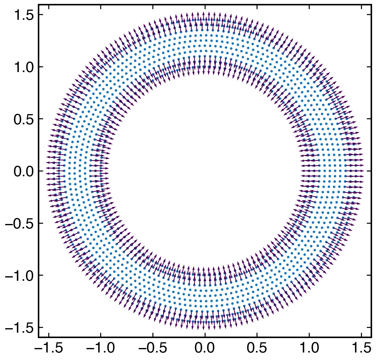
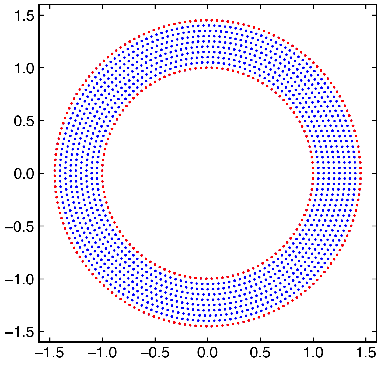
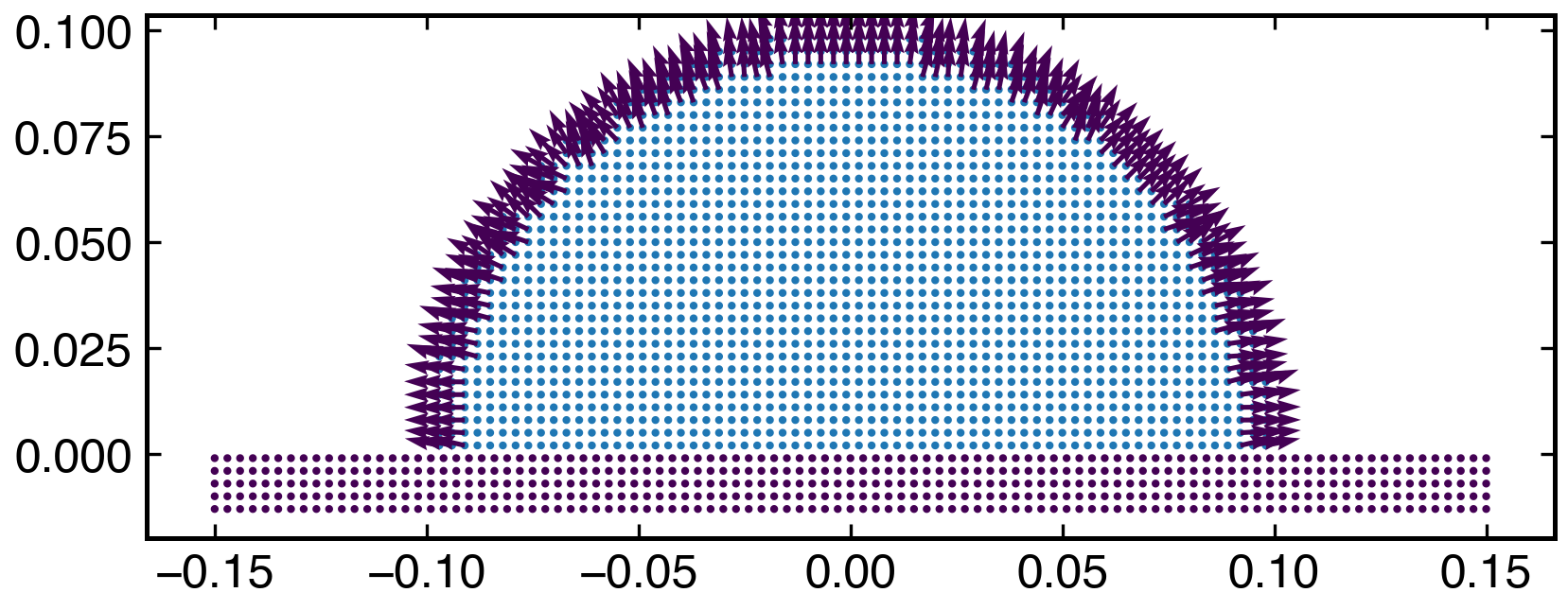
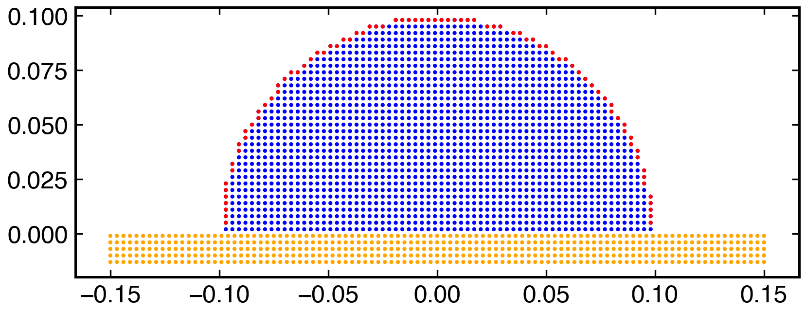
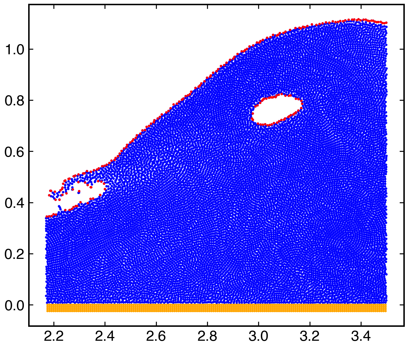
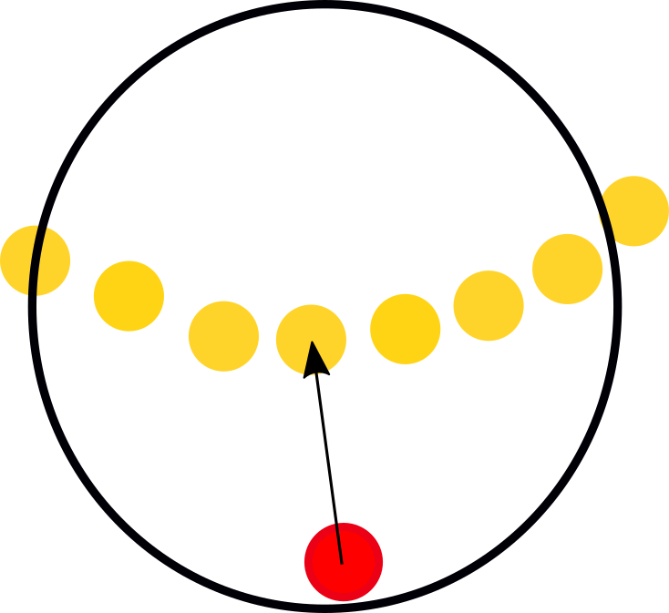
The current algorithm is tested with to two simple cases. We first consider a circular ring of fluid. As can be seen from fig. 1(a), three layers of particles which are near the free surface have a normal. From these normals we need to find the surface particles. We loop over all the particles in the medium, and any particles which have a non-zero normal are considered for further analysis. For each of these potential surface particles we find the angle between the particle and each of its neighbors. For a 2d case, if the angle between the normal of the particle and that of the line joining the particle to its neighbor is less than 60 degrees then this particle is not considered as a free-surface particle. If no such neighbor exists, then the particle is considered to be a free-surface particle. As can be seen in fig. 1(b), the free surface particles are correctly identified. As a second test case we consider a patch of fluid resting on a wall. As a first step we compute the normals of the particles, see fig. 2(a) and then loop over all the particles and by considering only the particles which have non-zero normals, we determine the boundary particles, as in fig. 2(b). Finally this is applied to the case of a dam break. As can be seen from fig. 3 and fig. 4, the free surface particles are identified correctly.

(a)

(b)

Figure 1: Identification of free surface particles of a circular ring of fluid. Depicts (a) normals of the fluid particles, (b) boundary particles of the fluid particles

(a)

(b)

Figure 2: Identification of free surface particles of a fluid resting on a wall. Depicts (a) normals of the fluid particles, (b) boundary particles of the fluid particles

Figure 3: Identification of normals of fluid in a dam break simulation. Shows us the normals of all the fluid particles

Figure 4: Identification of boundary particles of fluid at an instance in a dam break. Shows boundary particles of all the fluid particles

3.5 PST close to the free surface

Near the free-surface the PST has to be performed with some care for both fluids and solids. This is because of the lack of support for the particles near the free-surface. After the free surface particles are identified by using the algorithm described in section 3.4, we mark the particles which are in close proximity to the free surface particles. This is done through a variable associated with each particle called $h_{b}$, which is initialized to the initial smoothing length of the particles.

We loop over all the particles that are not on the boundary, and their $h_{b}$ is adjusted to the distance to the closest boundary particle divided appropriately by a kernel-dependent factor such that the kernel support is up to the closest boundary particle. In the current work, we have used a quintic spline kernel for which the factor is 3. The algorithm is shown in algorithm 1 and depicted in fig. 5(a). We note that this $h_{b}$ is only used for the PST force/displacement computation. This process allows us to ensure that the homogenization force does not push these particles towards the free-surface.

Algorithm 1 Algorithm to set $h_{b}$

1:for particle $i$ in all particles do

2:     if $i$ is a boundary particle then

3:         set $h_{b,i}=0$

4:     else

5:         set $h_{b,i}=h$      

6:for particle $i$ in all non-boundary particles do

7:     if particle $i$ has a boundary particle in its neighborhood then

8:         $x_{\text{dist},i}\leftarrow$ Distance to nearest boundary particle

9:         Set $h_{b,i}=\frac{x_{\text{dist, i}}}{3}$      

(a)

(b)

Figure 5: Set $h_{b}$ of the particles. (a) Particles with a free surface whose free particles are identified (b) Minimum distance between the particle in the vicinity of the free surface to the free surface particle.

In the PST of Sun et al. [20], the shifting acceleration is adjusted using

$$\bigg{(}\frac{d\mathbf{u}_{a}}{dt}\bigg{)}_{\text{c}}=\begin{cases}0&\text{if boundary},\\ \big{(}\frac{d\mathbf{u}_{a}}{dt}\big{)}_{\text{c}}-(\big{(}\frac{d\mathbf{u}_{a}}{dt}\big{)}_{\text{c}}\cdot\mathbf{n}_{a})\mathbf{n}_{a}&\text{if $h_{b}<h$},\\ \big{(}\frac{d\mathbf{u}_{a}}{dt}\big{)}_{\text{c}}&\text{if $h_{b}=h$}.\end{cases}$$ (44)

Whereas while using IPST [15], rather than adjusting the final shifting acceleration, we adjust the increment in the position of eq. 38,

$$\delta\mathbf{r}_{a}^{m}=\begin{cases}0&\text{if boundary},\\ \delta\mathbf{r}_{a}^{m}-(\delta\mathbf{r}_{a}^{m}\cdot\mathbf{n}_{a})\mathbf{n}_{a}&\text{if $h_{b}<h$},\\ \delta\mathbf{r}_{a}^{m}&\text{if $h_{b}=h$}.\end{cases}$$ (45)

3.6 Boundary conditions

The ghost particle approach of Adami et al. [34] is used to model the boundaries. We use three layers of ghost particles to model the solid wall. The properties of the solid wall are interpolated from the fluid particles.

When computing the divergence of the velocity field on fluid particles, we enforce a no-penetration boundary condition and not a no-slip boundary condition. The velocity of the fluid is projected onto the ghost particles using,

$$\mathbf{\hat{u}}_{a}=\frac{\sum_{b}\mathbf{u}_{b}W_{ab}}{\sum_{b}W_{ab}},$$ (46)

$$\mathbf{\check{u}}_{a}=\frac{\sum_{b}\tilde{\mathbf{u}}_{b}W_{ab}}{\sum_{b}W_{ab}},$$ (47)

where $\mathbf{u}_{b}$, $\mathbf{\tilde{u}}_{b}$ are the momentum and transport velocity of the fluid respectively and $W_{ab}$ is the kernel value between the fluid particle and the ghost particle.

The normal component of this projected velocity is then reflected and set as the ghost particle velocity,

$$\mathbf{u}_{\text{Ga}}=2\mathbf{\hat{n}}((\mathbf{u}_{\text{p}}-\mathbf{\hat{u}}_{\text{a}})\cdot\mathbf{\hat{n}})+\mathbf{\hat{u}}_{\text{a}},$$ (48)

where $\mathbf{u}_{\text{p}}$ is the local velocity of the boundary and $\mathbf{\hat{n}}$ is the unit normal to the boundary particle $a$. Similarly the transport velocity of the ghost particle is set as,

$$\tilde{\mathbf{u}}_{\text{Gi}}=2\mathbf{\hat{n}}((\mathbf{u}_{\text{p}}-\mathbf{\check{u}}_{\text{i}})\cdot\mathbf{\hat{n}})+\mathbf{\check{u}}_{\text{i}},$$ (49)

When the viscous force is computed, the no slip boundary condition is used, where the velocity on the boundary set as,

$$\mathbf{u}_{\text{Ga}}=2\mathbf{u}_{\text{p}}-\mathbf{\hat{u}}_{\text{a}},$$ (50)

a similar form is used for the transport velocity here too,

$$\tilde{\mathbf{u}}_{\text{Ga}}=2\mathbf{u}_{\text{p}}-\mathbf{\check{u}}_{\text{a}}.$$ (51)

The pressure of the boundary particle is extrapolated from its surrounding fluid particles by the following equation,

$$p_{w}=\frac{\Sigma_{f}p_{f}W_{wf}+(\mathbf{g}-\mathbf{a}_{\mathbf{w}})\cdot\Sigma_{f}\rho_{f}\mathbf{r}_{wf}W_{wf}}{\Sigma_{f}W_{wf}},$$ (52)

where $\mathbf{a}_{w}$ is the acceleration of the wall. The subscript $f$ denotes the fluid particles and $w$ denotes the wall particles.

For solid mechanics problems, in addition to the extrapolation of pressure, we also extrapolate the deviatoric shear stress on to the boundary particles using,

$$\sigma_{ij}^{{}^{\prime}}=\frac{\Sigma_{s}\sigma_{ij}^{{}^{\prime}}\;W_{ws}}{\Sigma_{s}W_{ws}},$$ (53)

where $s$ denotes the solid particles.

3.7 Time integration

We use the kick-drift-kick scheme for the time integration. We first move the velocities of the particles to half time step,

$$\mathbf{u}_{a}^{n+\frac{1}{2}}=\mathbf{u}_{a}^{n}+\frac{\Delta t}{2}\bigg{(}\frac{\tilde{d}\mathbf{u}_{a}}{dt}\bigg{)}^{n},$$ (54)

$$\mathbf{\tilde{u}}_{a}^{n+\frac{1}{2}}=\mathbf{u}_{a}^{n+\frac{1}{2}}+\frac{\Delta t}{2}\bigg{(}\frac{d\mathbf{u}_{a}}{dt}\bigg{)}^{n}_{c}.$$ (55)

Then the time derivatives of density and deviatoric stresses are calculated using the eq. 25 and eq. 4. The new time step density, deviatoric stresses and particle position are updated by,

$$\rho_{a}^{n+1}=\rho_{a}^{n}+\Delta t\;\bigg{(}\frac{\tilde{d}\rho_{a}}{dt}\bigg{)}^{n+\frac{1}{2}},$$ (56)

$$p_{a}^{n+1}=p_{a}^{n}+\Delta t\;\bigg{(}\frac{\tilde{d}p_{a}}{dt}\bigg{)}^{n+\frac{1}{2}},$$ (57)

$$\boldsymbol{\sigma}_{a}^{{}^{\prime}\;n+1}=\boldsymbol{\sigma}_{a}^{{}^{\prime}\;n}+\Delta t\;\bigg{(}\frac{\tilde{d}\boldsymbol{\sigma}^{{}^{\prime}}_{a}}{dt}\bigg{)}^{n+\frac{1}{2}},$$ (58)

$$\mathbf{r}_{a}^{n+1}=\mathbf{r}_{a}^{n}+\Delta t\;\mathbf{\tilde{u}}_{a}^{n+1}.$$ (59)

Finally, at new time-step particle position, the momentum velocity is updated

$$\mathbf{u}_{a}^{n+1}=\mathbf{u}_{a}^{n+\frac{1}{2}}+\frac{\Delta t}{2}\bigg{(}\frac{\tilde{d}\mathbf{u}_{a}}{dt}\bigg{)}^{n+1}.$$ (60)

For the numerical stability, the time step depends on the CFL condition as,

$$\Delta t=\mathrm{min}\bigg{(}0.25\;\frac{h}{c+|U|},0.25\;\frac{h^{2}}{\nu},0.25\;\frac{h^{2}}{g}\bigg{)},$$ (61)

where $|U|$ is the maximum velocity magnitude, $c$ is the speed of sound typically chosen as $10|U|$ for fluids in this work.

For solid mechanics, the timestep is set based on the following,

$$\Delta t\leq 0.25\;\bigg{(}\frac{h}{c_{0}+|U|}\bigg{)},$$ (62)

where $c_{0}$ is the speed of sound of the solid body.

4 Results

We validate the proposed scheme using a suite of benchmark problems for both fluid and solid mechanics. We first consider fluids where we look at the Taylor-Green vortex problem, the lid-driven cavity, and the two-dimensional dam-break problem. We then consider problems in elastic dynamics like the oscillating plate, a uniaxial compression problem, the collision of rubber rings, and a high-velocity impact problem.

We show how the proposed method is an improvement on previous work. Every result shown is produced using an automation framework [26]. The source code is available at https://gitlab.com/pypr/ctvf.

4.1 Taylor-Green vortex

In the first benchmark, we test the accuracy of the correction terms and evaluate the different particle shifting schemes introduced in the proposed scheme by simulating a Taylor-Green vortex. It consists of a periodic unit box with no solid boundaries. Taylor-Green vortex problem has an exact solution given as,

$$u =-Ue^{bt}\cos(2\pi x)\sin(2\pi y)$$ (63)

$$v =Ue^{bt}\sin(2\pi x)\cos(2\pi y)$$ (64)

$$p =-U^{2}e^{2bt}(\cos(4\pi x)+\cos(4\pi y))/4,$$ (65)

where $U$ is chosen as $1$ m s^-1, $b=-8\pi^{2}/Re$, $Re=UL/\nu$, and $L=1$ m. We initialize the fluid using this at $t=0$ and compare the results with the exact solution. The Reynolds number, $Re$, is initially chosen to be $100$. The quintic spline with $h/\Delta x=1.0$ is used. We use summation density to compute the density and evolve pressure with eq. 26. No artificial viscosity is used for this problem. The decay rate of the velocity is studied using the evolution of maximum velocity $|\mathbf{u}_{\max}|$ in time. We compute the $L_{1}$ error in the velocity magnitude as,

$$L_{1}=\frac{\sum_{i}|\mathbf{u}_{i,computed}|-|\mathbf{u}_{i,exact}|}{\sum_{i}|\mathbf{u}_{i,exact}|},$$ (66)

where $\mathbf{u}_{i,exact}$ is found at the position of the $i$’th particle.

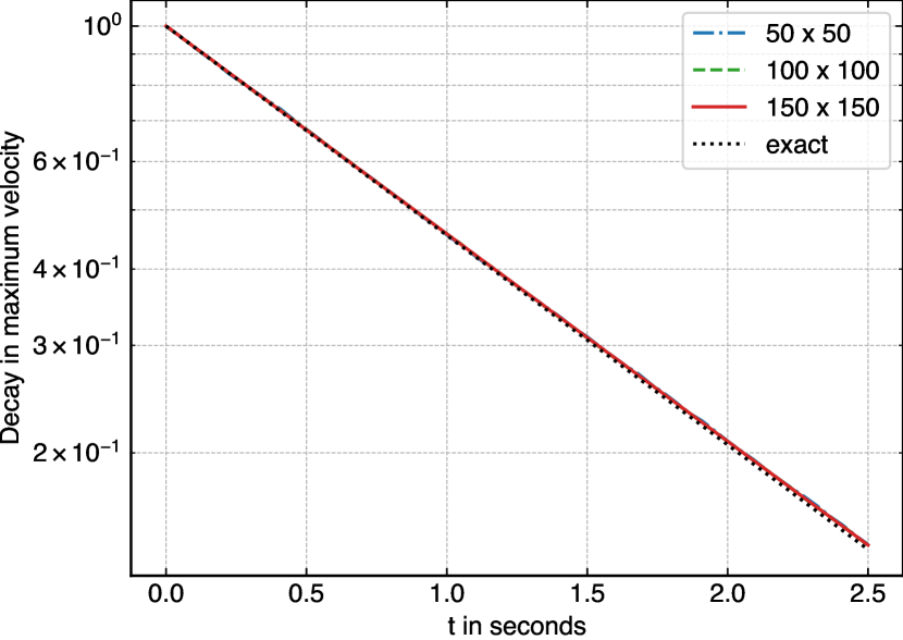
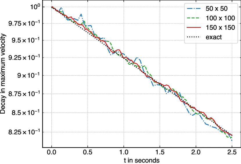
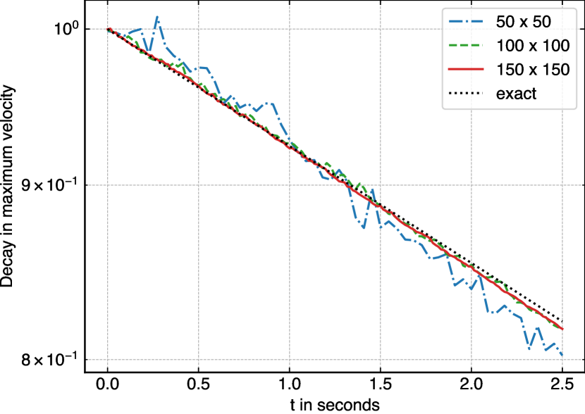
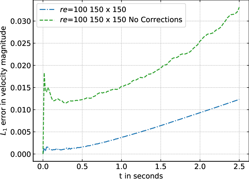
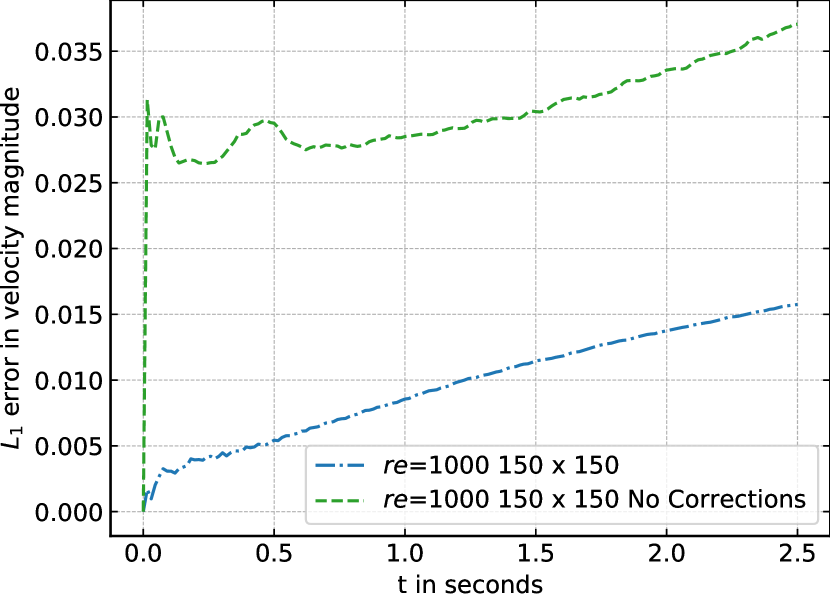
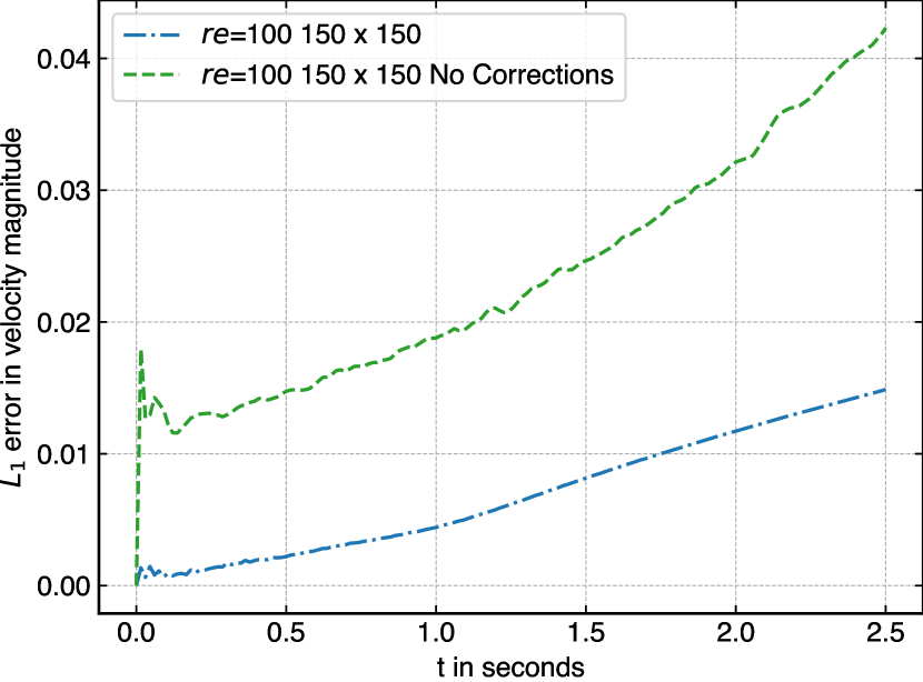
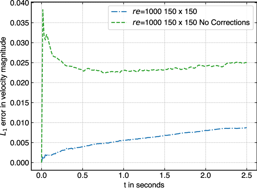
In fig. 6(a) we compare the decay of $|\mathbf{u}_{\max}|$ with that of the exact solution for the case where we use SPST for particle shifting. As can be seen, the results are in excellent agreement with the expected decay. The same is seen in fig. 7(a) for the case using IPST. This shows the accuracy and robustness of the scheme with respect to changing the PST method. Figure 6(b) and fig. 7(b) show the $L_{1}$ error of velocity magnitude for various resolutions simulated using the two PST techniques. Figure 10 depicts the $L_{1}$ error of velocity magnitude for a Reynolds number of 100 and 1000 using SPST with and without correction terms. Figure 11 shows the same but using the IPST. The improvement due to the correction terms is clearly seen as a significant reduction in the error.

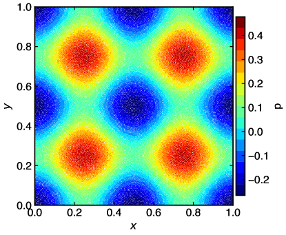
One can see that the IPST has lower errors at initial times. However, we do note that there appears to be a lack of convergence in the result as the resolution is increased. As the number of particles is increased the $L_{1}$ error does not correspondingly reduce. This is due to the low Reynolds number and the discretization of the viscous term that is being used. We show the results of the velocity decay and the $L_{1}$ error when a Reynolds number of 1000 is used in fig. 8 for IPST and in fig. 9 with SPST. In this case the convergence is clearly seen as the resolution is increased. Figure 12 shows distribution of particles with the color representing pressure. The Reynolds number of 1000 with a resolution of 150$\times$150. We can see that the pressure distribution is smooth.

(a)

(b)

Figure 6: Taylor-Green vortices for an initial particle distribution of $50\times 50$, $100\times 100$ and $150\times 150$ is simulated with a Reynolds number of 100 using SPST. Plots shown are (a) decay in maximum velocity (b) $L_{1}$ error in velocity magnitude.

(a)

(b)

Figure 7: Taylor-Green vortices for an initial particle distribution of $50\times 50$, $100\times 100$ and $150\times 150$ is simulated with a Reynolds number of 100 using IPST. Plots shown are (a) decay in maximum velocity (b) $L_{1}$ error in velocity magnitude.

(a)

(b)

Figure 8: Taylor-Green vortices for an initial particle distribution of $50\times 50$, $100\times 100$ and $150\times 150$ is simulated with a Reynolds number of 1000 using IPST. Plots shown are (a) decay in maximum velocity (b) $L_{1}$ error in velocity magnitude.

(a)

(b)

Figure 9: Taylor-Green vortices for an initial particle distribution of $50\times 50$, $100\times 100$ and $150\times 150$ is simulated with a Reynolds number of 1000 using SPST. Plots shown are (a) decay in maximum velocity (b) $L_{1}$ error in velocity magnitude.

(a)

(b)

Figure 10: $L_{1}$ error for nx with 150 $\times$ 150 with and without corrections with SPST with a Reynolds number of a) 100 and b) 1000

(a)

(b)

Figure 11: $L_{1}$ error for nx with 150 $\times$ 150 with and without corrections with IPST with a Reynolds number of a) 100 and b) 1000

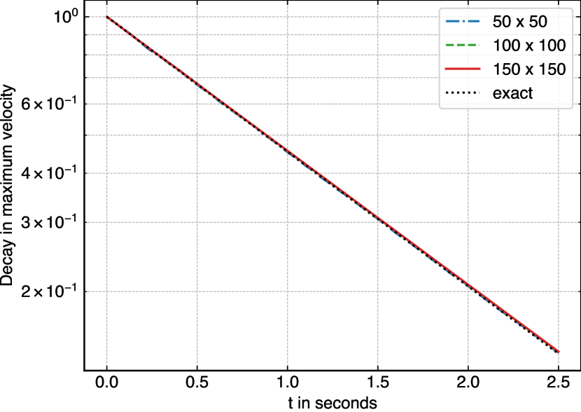
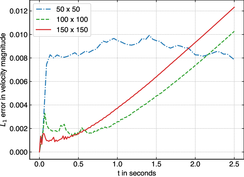
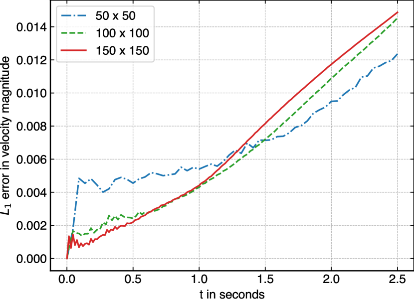
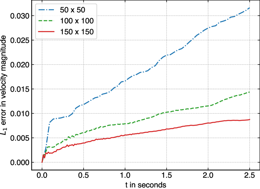
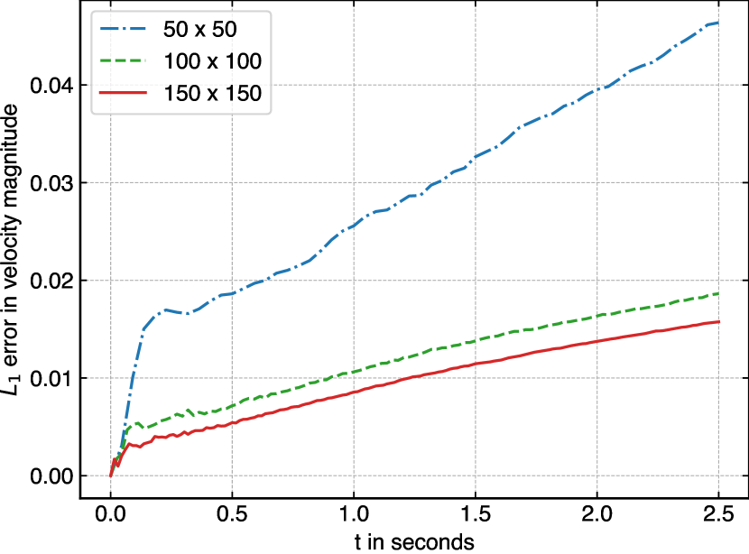
An inspection of figures 6(b), 7(b) and 8(b), 9(b) suggests that the IPST appears to be better than that of SPST.

Figure 12: Particle plot of Taylor green vortices for a Reynolds number of 1000 with a resolution of $150\times 150$. The colors represent the pressure.

4.2 Lid driven cavity

We evaluate the ability of the proposed scheme to handle solid wall boundary conditions by simulating a lid-driven cavity. The lid-driven cavity is a classic problem that can be challenging to simulate in the context of the SPH. It has been simulated by [17], [15], [21] to note a few. A rectangular cavity with length 1 m which is filled with fluid is constrained by four walls. Top wall has a velocity of $U=1$ m s^-1. A unit density is assumed for the fluid. The speed of sound of the fluid particle is set to $c=10U_{max}$. We use the summation density to compute the density. The viscosity of the fluid is set through the Reynolds number of the flow, $\nu=\frac{Re}{U}$. No artificial viscosity is used in the current problem.

Figure 13: Particle plot of cavity with a $Re=100$ with particle arrangement of $150\times 150$, left side with corrections and right side without correction terms.

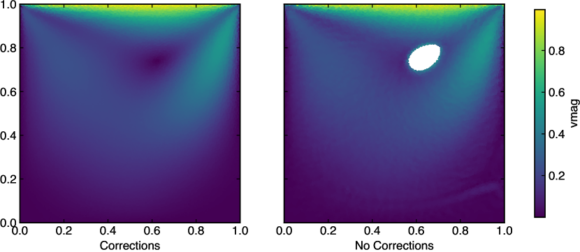
We first simulate the cavity problem with a Reynolds number of 100 with and without corrections. In fig. 13 we can see that an unphysical void is produced when no corrections are employed. This is eliminated with the current scheme.

Figure 14: Velocity profiles $u$ vs. $y$ and $v$ vs. $x$ for the lid-driven-cavity problem at $Re=100$ with three initial particle arrangement of $50\times 50$, $100\times 100$, and $150\times 150$.

Figure 15: Velocity profiles for the lid-driven-cavity using the steady state simulation procedure for $Re=1000$ with initial partial arrangement of $50\times 50$, $100\times 100$, and $200\times 200$ compared with the results of [35].

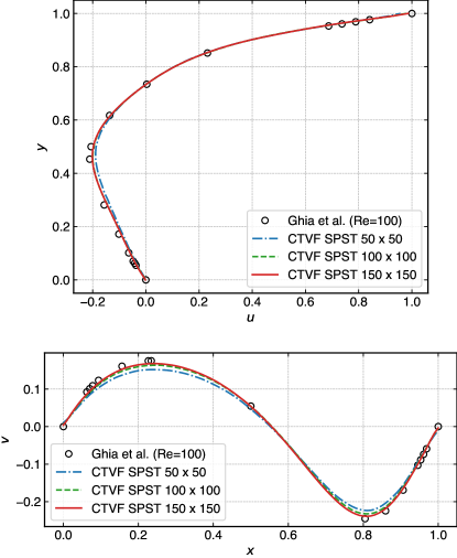
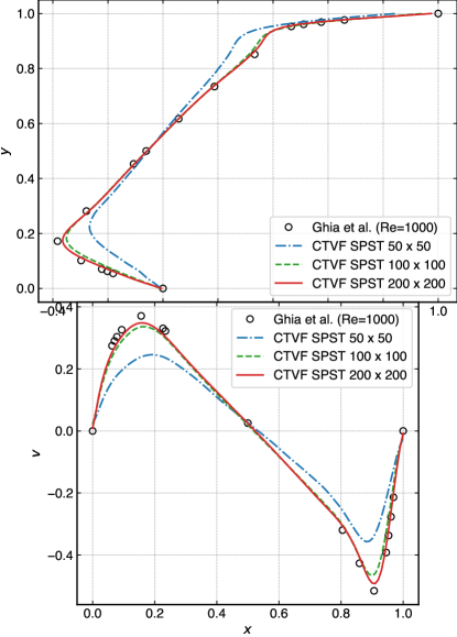
We now study convergence of the method as we vary the resolution. Figure 14 and fig. 15 show the center-line velocities $u$ versus $y$ and $v$ versus $x$ for the Reynolds numbers 100 and 1000 respectively. For the $Re=100$ case we use three different resolutions of $50\times 50,100\times 100$ and $150\times 150$. For the $Re=1000$ case, we use an initial $50\times 50$, $100\times 100$, and $200\times 200$ grid of particles. These are compared against the results of [35]. As we can see that the current scheme is able to predict the velocity profiles well.

4.3 2D Dam-break

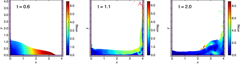
We apply the proposed scheme to free surface flows by simulating a dam-break. This problem has been extensively studied before for example in [33], [18], and [21].

A block of fluid having width 1m and a height of $2$ m is allowed to settle under the influence of gravity inside a tank of length $4$ m. The fluid block is initially placed to the left of the tank. The acceleration due to gravity is $g=9.81$ m s^-2. To simulate the free surface flows we use the continuity equation to evolve the density using (25) and the (26) to evolve the pressure. We use free slip boundary conditions to compute the divergence of the velocities and a no-slip boundary condition while computing the viscous forces. The value of $\alpha=0.05$ is used for the artificial viscosity eq. 28 term.

Figure 16: Position of the toe of the water versus time of CTVF as compared with the simulation of  [36]. Z is the distance of toe of the dam from the left wall and L is the initial width of the dam

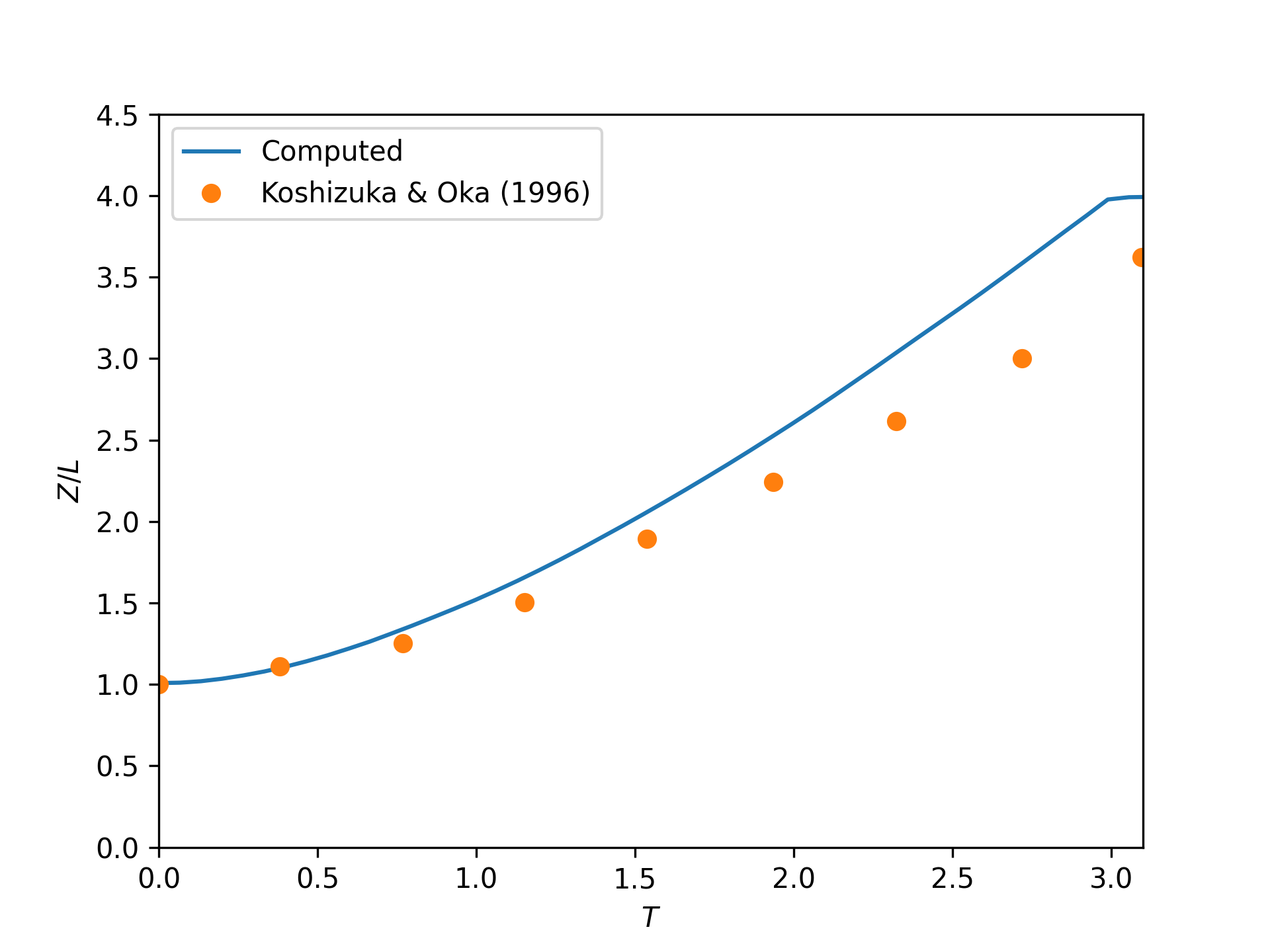
Figure 16 compares the position of the toe of the fluid block with time against [36], where the authors use the moving particle semi-implicit scheme to simulate the same.

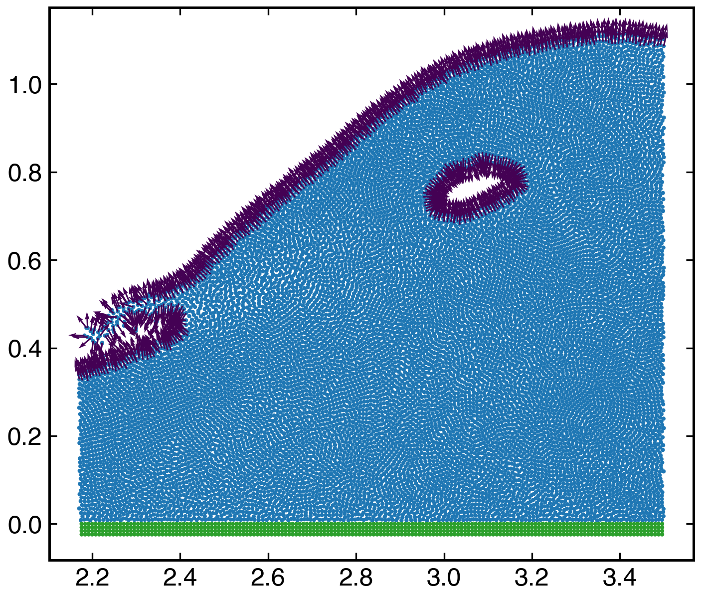
The evolution of the fluid at three different time instants t$=0.6,1.1,2.0$ seconds, is shown in fig. 17. As can be seen from fig. 17, at time $2.0$ seconds we have captured the void created due to the splashing of the fluid. The colors in fig. 17 shows the velocity magnitude.

Figure 17: Particle plots of fluid in dam break at time $t=0.6,1.1,2.0$ second, showing velocity magnitude as contour.

4.4 Oscillating plate

In this section, we test the improvement due to the correction terms while simulating elastic solids. We show the elimination of tensile instability while extending the transport velocity formulation [17] scheme to more particle shifting techniques. We consider a thin oscillating plate that is clamped on one side. Landau et al. [37] provide an analytical solution for this problem. This is also simulated numerically in [7] and [18].

An oscillating plate with a length of $0.2$ m and a height of $0.02$ m is initially given with a velocity profile of,

$$v_{y}(x)=V_{f}\,c_{0}\frac{F(x)}{F(L)},$$

where $V_{f}$ varies for different cases. $L$ is the length of the plate. $F(x)$ is given by,

$$F(x)=(\cos(kL)+\cosh(kL))\,(\cosh(kx)-\cos(kx))+\\ (\sin(kL)-\sinh(kL))\,(\sinh(kx)-\sin(kx)).$$ (67)

In the present example $kL$ is 1.875. The material properties of the plate are as follows, Young’s modulus $E=2.0\times 10^{6}$ Pa, a Poisson’s ratio of $\nu=0.3975$. $c_{0}$ is speed of sound, and a density of $\rho=1000$ kg m^-3, as done in [7]. In all the cases simulated here, we use an $\alpha$ of $1$ for artificial viscosity.

The GTVF [18] eliminates the tensile instability while using the special PST proposed in the original paper. We show that the GTVF [18] scheme is unable to eliminate numerical fracture when a different PST algorithm is employed. Instead of using the standard GTVF homogenization acceleration we use Sun’s particle shifting technique (SPST). This results in a numerical fracture, as seen in fig. 18(b). We reproduced the same case with original GTVF scheme, where no numerical fracture has found as seen in fig. 18(a). This numerical fracture is eliminated by the current scheme. This is due to the incorporation of the additional terms in the current scheme as well as the use of momentum velocity in the computation of the velocity gradient. Note that a particle spacing of $\Delta x=0.002$ m and $V_{f}=0.05$ m s^-1 has been used.

(a)

(b)

Figure 18: Oscillating plate with a length of $0.2$m and height of $0.02$m when simulated with GTVF Scheme. Figure in left is original GTVF scheme and right is while using SPST with GTVF scheme.

This is further demonstrated by a case where an oscillating plate of length of $0.2$ m and a height of $0.02$ m is simulated for a time of $0.22$ seconds. Similarly, another case where plate of height $0.01$ m and a width of $0.2$ m is run for a time of $0.51$ s. Figure 19 and fig. 20 shows particles of the plate at time $t=0.22$ s and $0.51$ s of these two cases respectively. As we can see from the figure that the plate is free of numerical fracture, thus the tensile instability is eliminated.

Figure 19: Oscillating plate at time $t=0.22$s with a length of $0.2$m and height of $0.02$m simulated with SPST with CTVF scheme.

Figure 20: Oscillating plate at time $t=0.51$s with a length of $0.2$m and height of $0.01$m simulated with SPST with CTVF scheme.

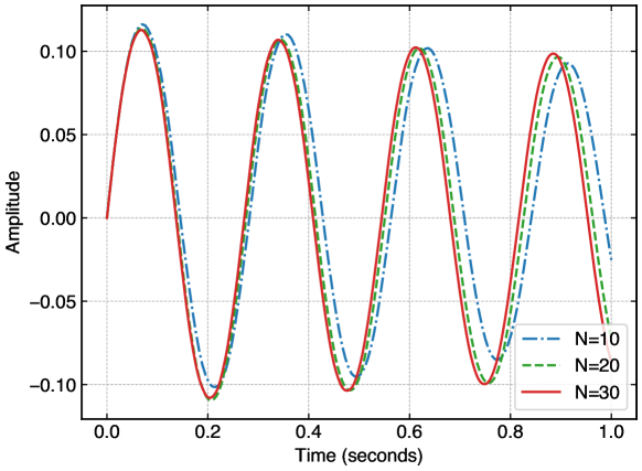
The accuracy of the current scheme is evaluated by comparing with the analytical results and with a convergence study. In table 1 we compare the time period for the oscillation by the analytical and the numerical results with varying $V_{f}$, where we consider an oscillating plate whose $H/L$ ratio is $0.1$. The difference between the analytical result and the numerical result is due to the fact that the analytical results are based on thin plate theory where as the plate considered here has a finite thickness. Further, we can see that the current numerical results are in agreement with the previously reported numerical results [7, 18]. In fig. 21, we have performed a convergence study of an oscillating plate, with a $\nu=0.3975$, and $V_{f}=0.05$ m s^-1, and IPST is used for particle homogenization. The trend of the current scheme matches well with the other updated Lagrangian SPH schemes [7, 18]. Hence the current scheme is able to work with different PST methods and remove the tensile instability.

$V_{f}$	0.001	0.01	0.03	0.05
$\text{T}_{\mathrm{CTVF}}$	0.284	0.283	0.283	0.284
$\text{T}_{\mathrm{GTVF}}$	0.284	0.283	0.284	0.285
$\text{T}_{\mathrm{analytical}}$	0.254	0.252	0.254	0.254

Table 1: Comparison between the CTVF and the analytical solution for the time period of the oscillating plate with a length of $0.2$m and height of $0.02$m with various $V_{f}$

Figure 21: The vertical position of the particle at the end of the plate as a function of time. Here we consider a three particle variations, 10, 20 and 30 particles across the plate width.

4.5 Uniaxial compression

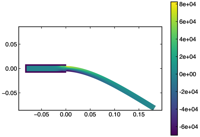
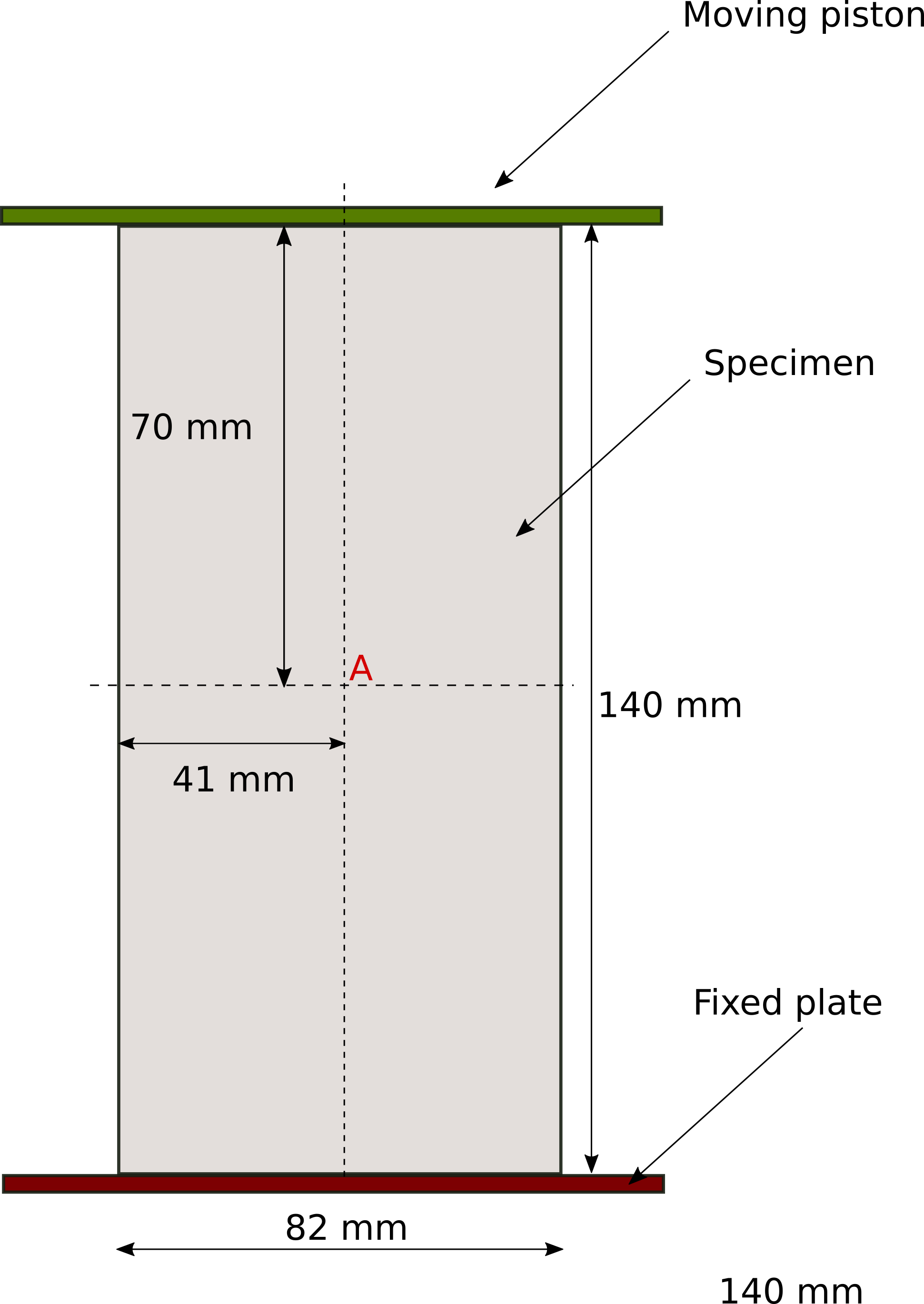
This benchmark is used to test the proposed scheme. A uniaxial bar is compressed by a moving piston on top of it. This problem has been simulated by Das and Cleary [38]. We compare the von Mises stress at the center point of the bar with the result of the FEM analysis and SPH provided in [38].

The numerical model consists of three parts. It has an axially loaded rectangular specimen of width $82$ mm and height of $140$ mm. The specimen has the properties of a sand stone (Crossley Sandstone) with a Young’s modulus of $7.5$ GPa and Poisson ratio of $0.398$ and with a density of $2300$ kg m^-3. The speed of sound resulting from such properties is $2303$ m s^-1. We run three particle resolutions, $\Delta x=0.5$ mm, $1$ mm and $2$ mm. The particles are placed on a regular square grid pattern. The velocity of the top plate is $1.5$ mm s^-1, which is used to apply the load on the specimen in such a fashion, such that the loaded end is deformed at the required constant rate. This is described in fig. 22. An $\alpha$ of $1$ is used in the current simulation for the artificial viscosity.

Figure 22: Test configuration of sand stone under uniaxial compression.

We use the von Mises stress as the criterion for analysing the stress field. It combines the normal and shear components of the deviatoric stress tensor, and is a commonly used criterion to assess failure strength of materials. The von Mises stress $\sigma_{vm}$ can be expressed in 2D in terms of principle stress $\sigma_{1}$ and $\sigma_{2}$ as

$$\sigma_{vm}=\sqrt{\left(\sigma_{1}^{2}+\sigma_{2}^{2}-\sigma_{1}\ \sigma_{2}\right)}$$ (68)

Where the principal stress are found by

$$\sigma_{1}=\frac{\sigma_{xx}+\sigma_{yy}}{2}+\sqrt{\left(\bigg{(}\frac{\sigma_{xx}+\sigma_{yy}}{2}\bigg{)}^{2}+\sigma_{xy}^{2}\right)}$$ (69)

$$\sigma_{2}=\frac{\sigma_{xx}+\sigma_{yy}}{2}-\sqrt{\left(\bigg{(}\frac{\sigma_{xx}+\sigma_{yy}}{2}\bigg{)}^{2}+\sigma_{xy}^{2}\right)}$$ (70)

Figure 23: von Mises stress at point A in uniaxial compression with three different resolutions compared against those from [38].

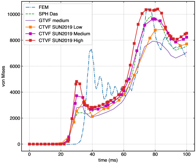
Figure 23 shows the von Mises stress versus time of the current scheme, when simulated with three different resolutions compared against with the finite element result and SPH result provided in [38]. It also shows the result with the GTVF scheme using the medium resolution. As can be seen in fig. 23 the GTVF result does not match very well with FEM and SPH result provided by Das and Cleary [38], and the current scheme performs significantly better.

4.6 Colliding Rings

Having shown the flexibility of proposed scheme to work with different PST methods in section 4.4, in the current example, we compare the robustness of the PST methods by investigating the collision of rubber rings with different Poisson ratios. This was first studied in SPH by Swegle et al. [39].

The inner ring radius of the ring is $r_{min}=0.03$ m and the outer ring radius $r_{max}=0.04$ m. Both the rings have the same material properties: Young’s modulus $E=0.01$ GPa and density $\rho=1.2\times 10^{3}$ kg m^-3. The initial speed of the rings are equal to $v_{0}=0.12c_{0}$ m s^-1 with an initial inter particle spacing of $\Delta x=0.001$ m. Where $c_{0}$ is the speed of sound of the material. We use an $\alpha=1$ for the artificial viscosity in the current simulation.

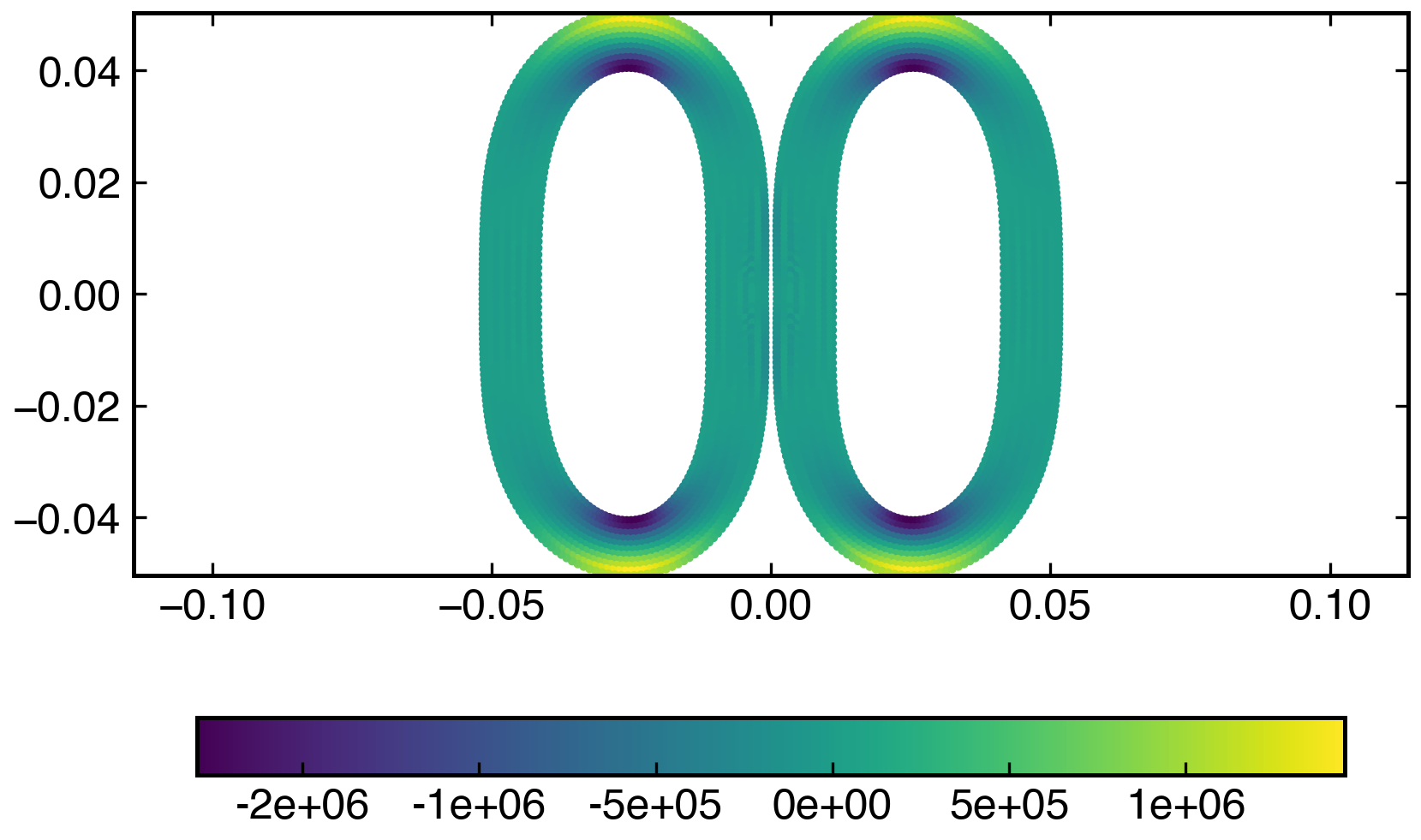
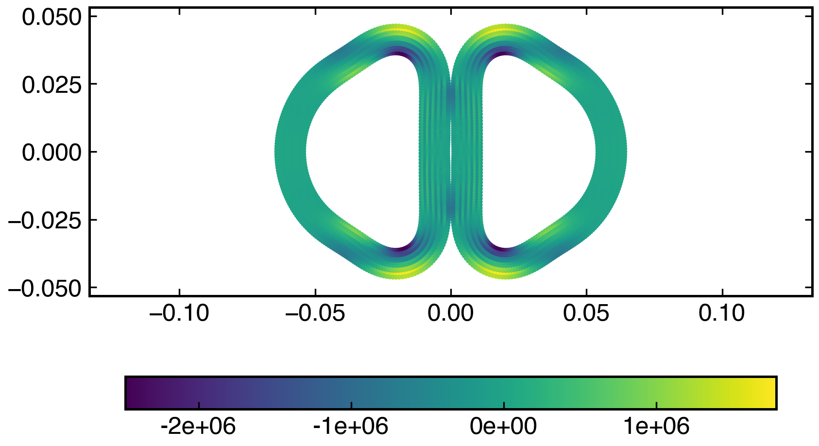
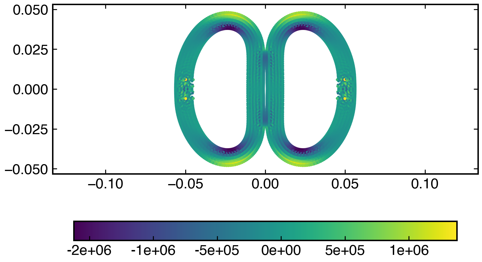
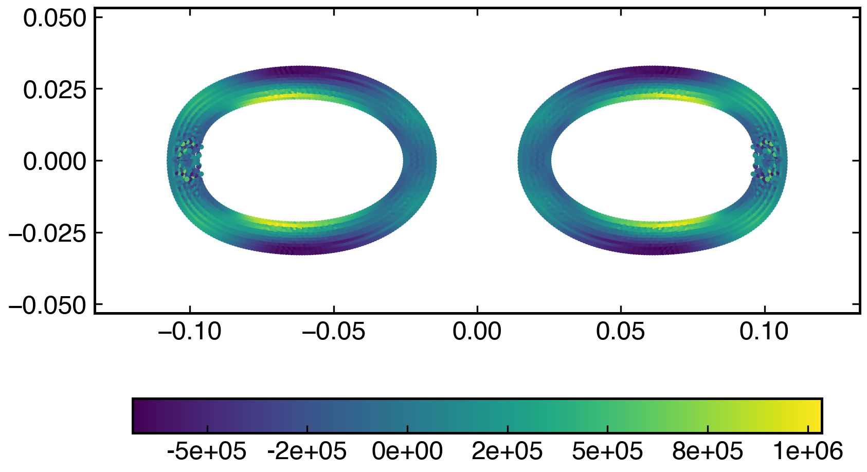
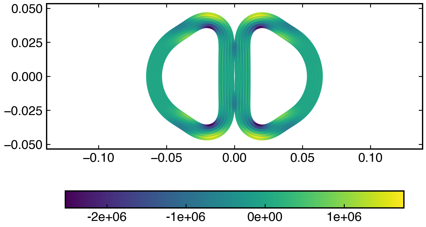
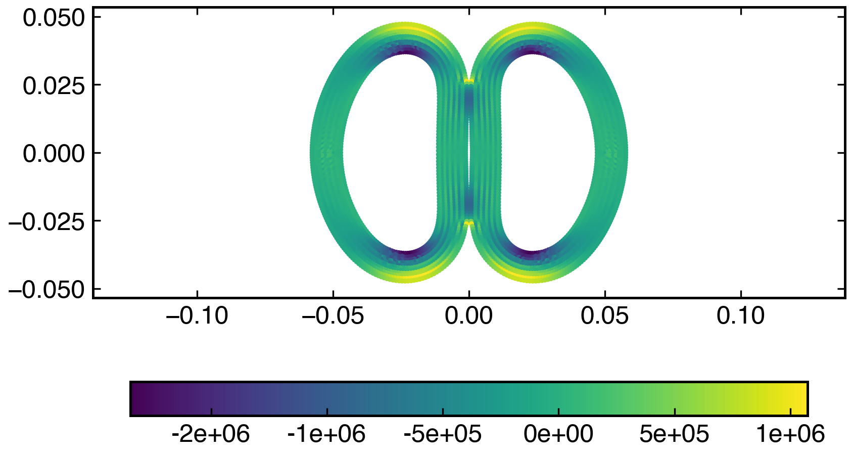
Two different Poisson ratios are simulated. Figure 24 shows the particle positions of rings with a Poisson ratio of $0.3975$ when simulated with SPST. The recovery of the colliding rings without any tensile instability can be seen.

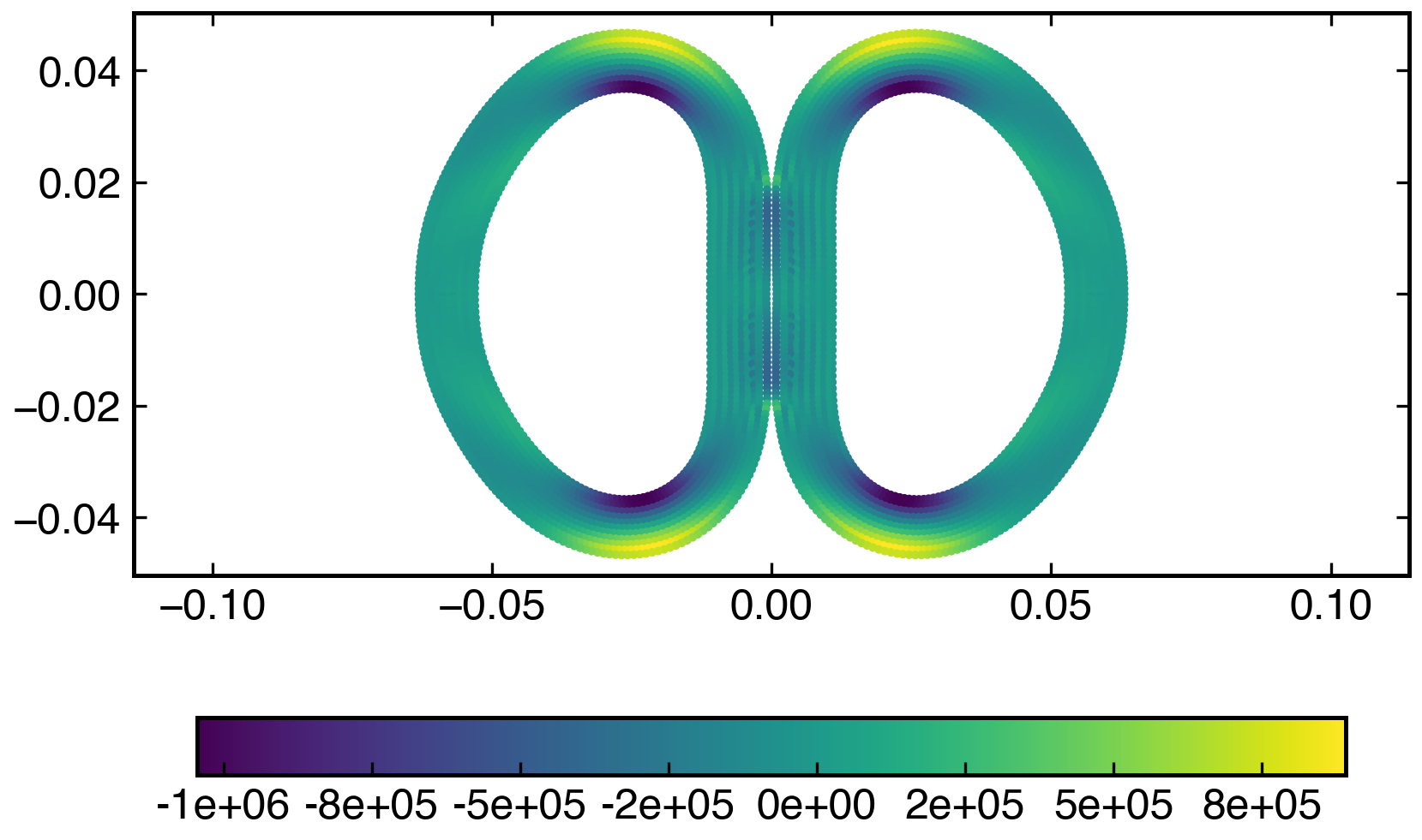
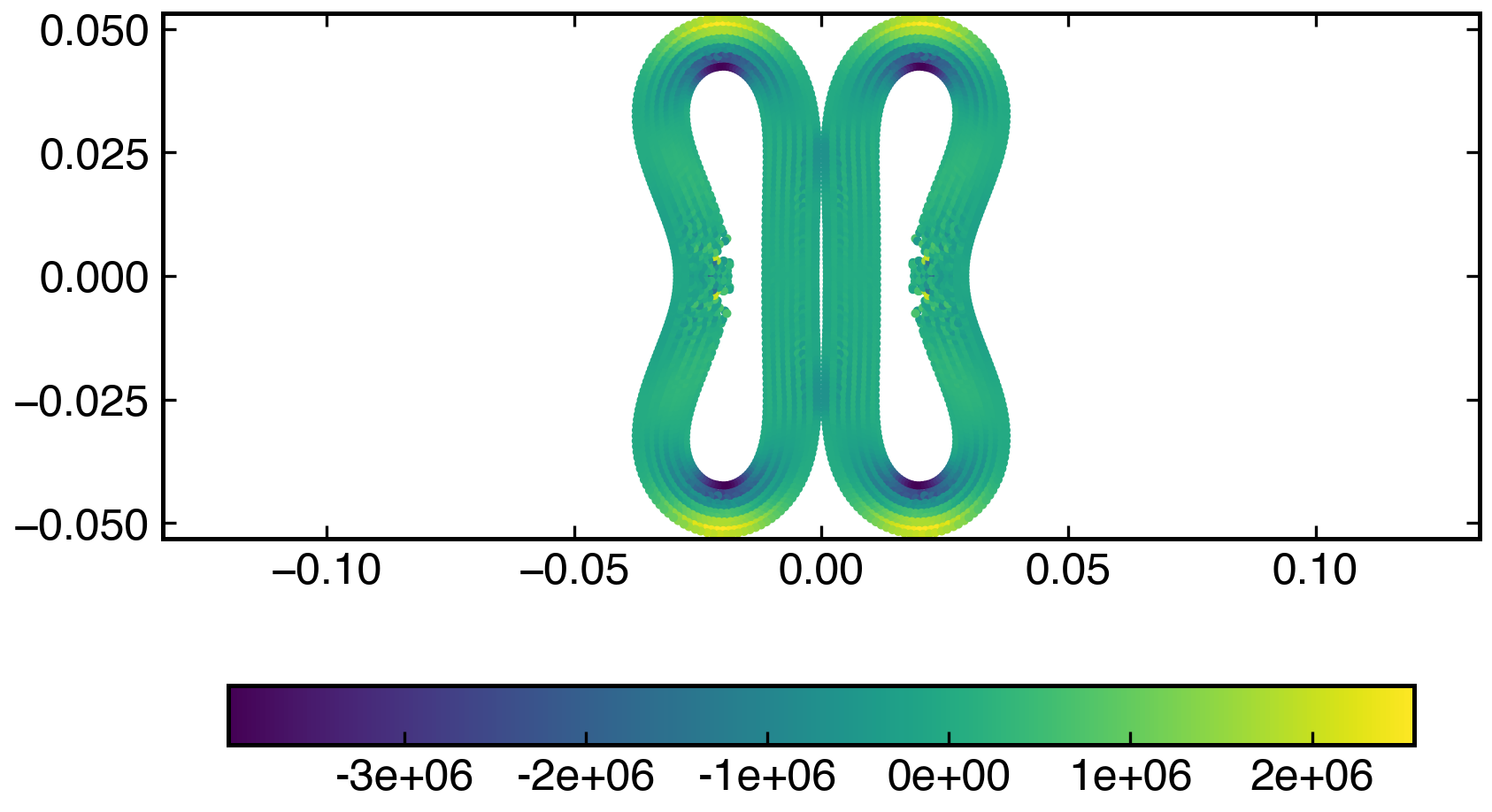
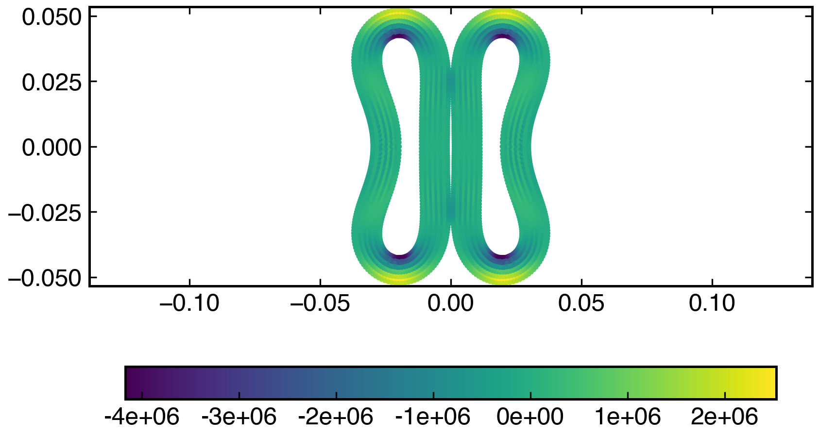
We also consider higher Poisson ratios, such as 0.47. Figure 25 shows the particle positions of rings when simulated with SPST and fig. 26 with IPST. Even though both the particle shifting techniques are able to eliminate the numerical fracture, IPST gives better results as in the distribution of particles through out the simulation, see fig. 25(b) and fig. 26(b). For the case where SPST is used, the final particle distribution is not very uniform. This is not the case when IPST is used. We can therefore say that IPST performs better than SPST.

(a) t = 2.5e-03 sec

(b) t = 4e-03 sec

(c) t = 7.3e-03 sec

(d) t = 1.45e-02 sec

Figure 24: Rings with a Poisson ratio of 0.3975 colliding head on, simulated with CTVF using SPST.

(a) t = 2.5e-03 sec

(b) t = 4e-03 sec

(c) t = 7.3e-03 sec

(d) t = 1.45e-02 sec

Figure 25: Rings with a Poisson ratio of 0.47 colliding head on, simulated with CTVF using SPST.

(a) t = 2.5e-03 sec

(b) t = 4e-03 sec

(c) t = 7.3e-03 sec

(d) t = 1.45e-02 sec

Figure 26: Rings with a Poisson ratio of 0.47 colliding head on, simulated with CTVF using IPST.

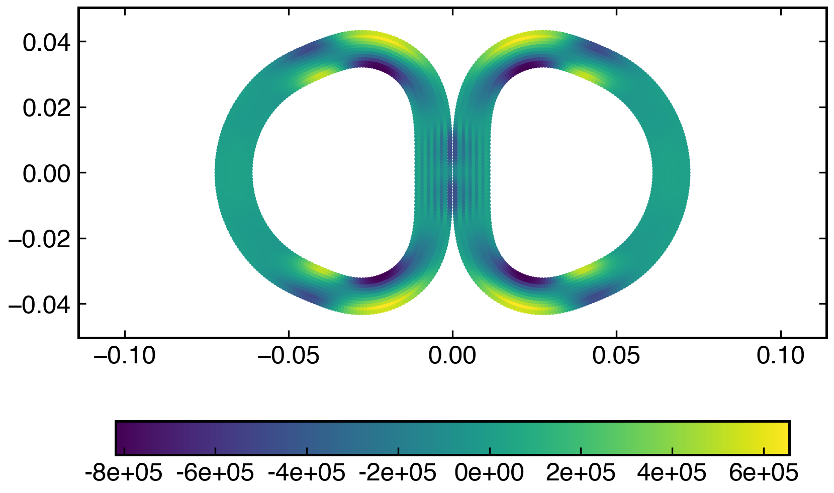
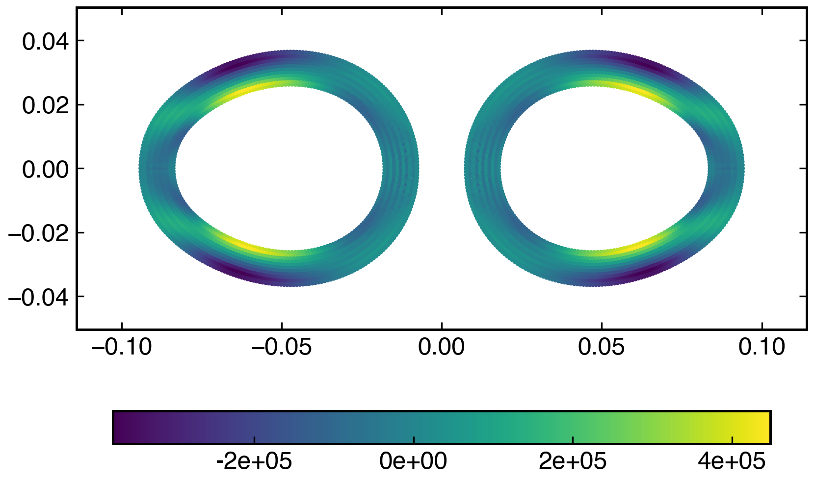
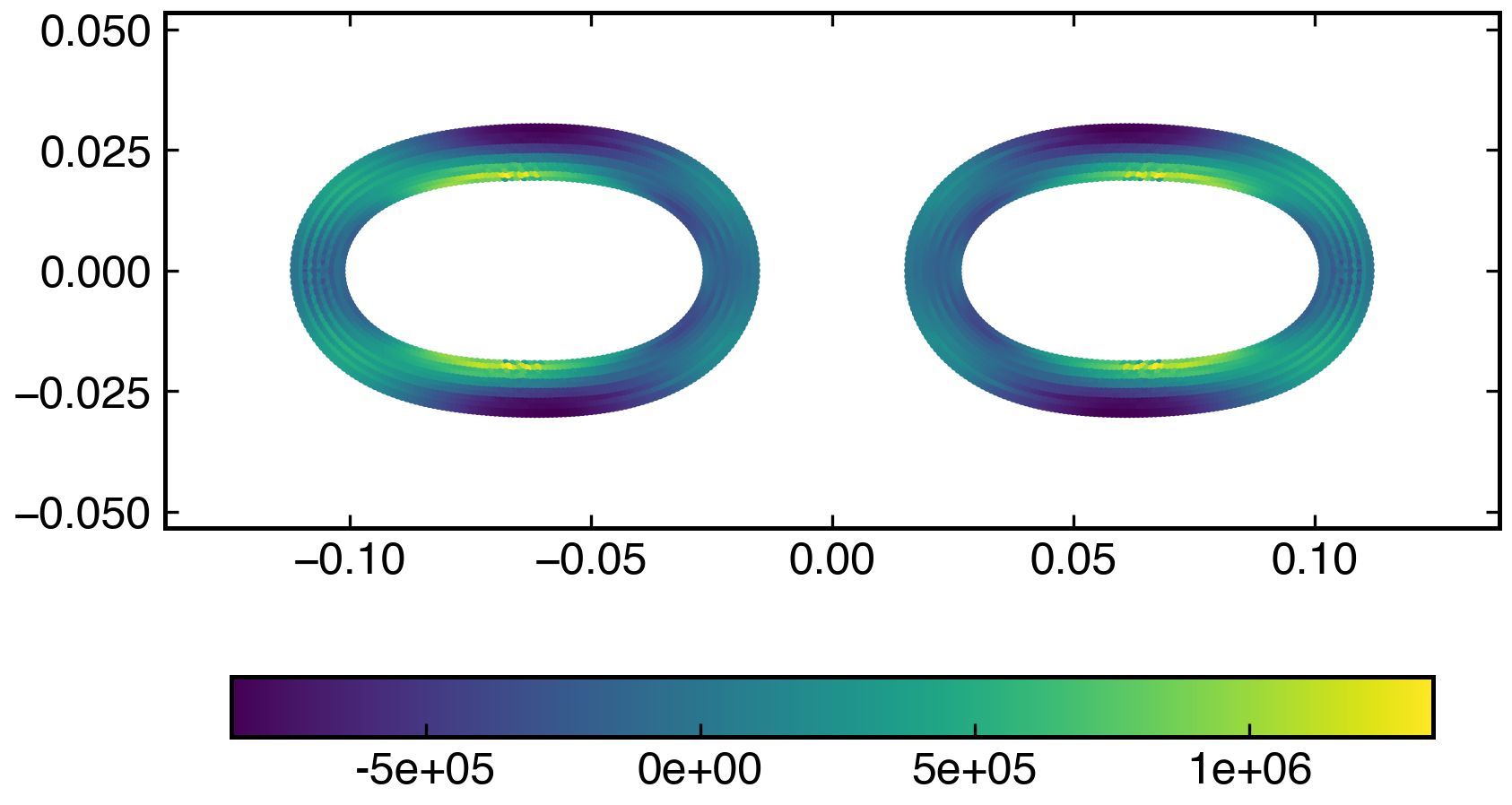
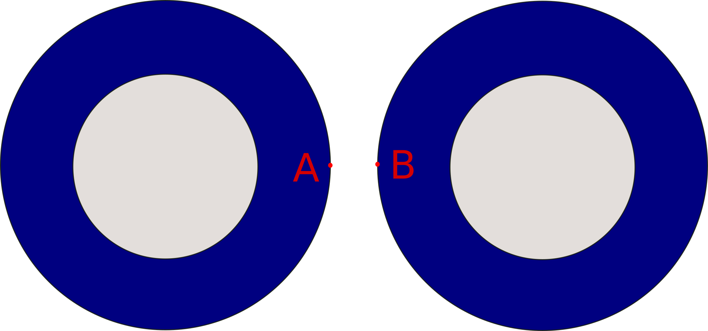
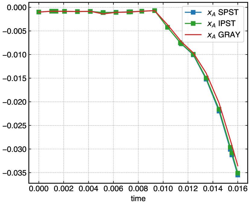
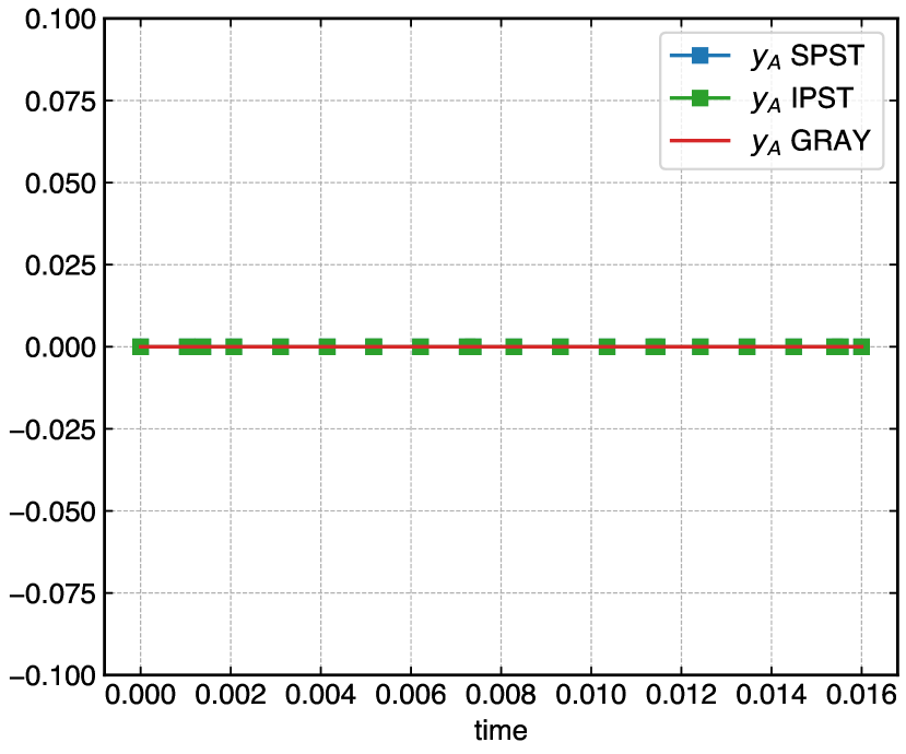
In order to compare the different schemes quantitatively for this problem, we plot the $x$ and $y$ positions of the point A of the left ring, as can be seen in fig. 27. Figure 28 shows the results and as can be seen excellent agreement of the different methods for this problem.

Figure 27: Schematic diagram of two rings colliding. Points A and B are marked.

(a) $x$ coordinate of the point A

(b) $y$ coordinate of the point A

Figure 28: The evolution of the $x$ and $y$ coordinates of points A and B for the CTVF using SPST, IPST, and compared with that of Gray [7].

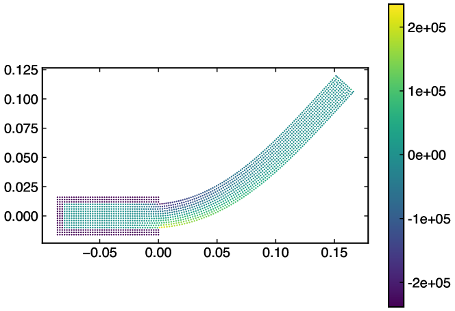
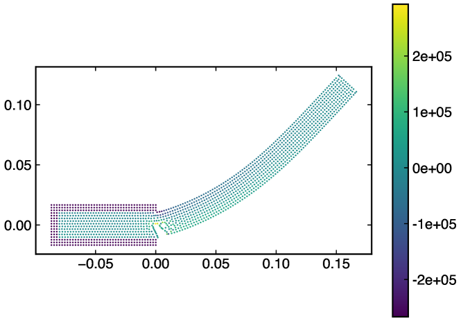
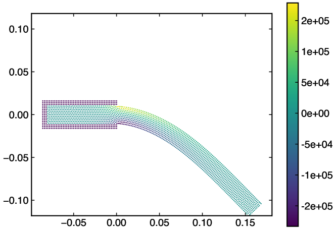
4.7 High velocity impact

High-velocity impact problems are important in various contexts like space debris applications. This case tests if the scheme is capable of hand large deformation problems.

The projectile and the target are made of aluminium material. The projectile is 10mm in diameter and the rectangular target has a size of $2\times 50$ mm. The projectile and the target have the following material properties: density $\rho=2785$ kg m^-3, sound speed $c_{0}=5328$ m s^-1, shear modulus $G=2.76\times 10^{7}$ kPa, yield modulus $Y_{0}=3.0\times 10^{5}$ kPa, as studied in [18]. The impact velocity is set to $V_{0}=3100.0$m s^-1. The initial particle spacing is $\Delta x=0.5$ mm.

(a) t = 0 sec

(b) t = 2.5e-03 sec

(c) t = 4e-03 sec

(d) t = 7.3e-03 sec

(e) t = 1.45e-02 sec

(f) t = 1.5e-02 sec

(g) t = 1.5e-02 sec

(h) t = 1.5e-02 sec

(i) t = 1.5e-02 sec

Figure 29: High velocity impact of cylinder on to a structure

Here the aluminium follows an elastic-perfectly plastic constitutive model. In elastic perfectly plastic model, the material is assumed to be elastic up to the yield point and once the material reaches the yield point, there will be no further increase in the stress, and is bounded by a factor $\beta=\min\left(\frac{Y_{0}^{2}}{3J_{2}},1\right)$, where $J_{2}$ is calculated from $J_{2}=\frac{1}{2}\boldsymbol{\sigma}^{{}^{\prime}}:\boldsymbol{\sigma}^{{}^{\prime}}$. We use an $\alpha=1$ in eq. 28 in the current case.

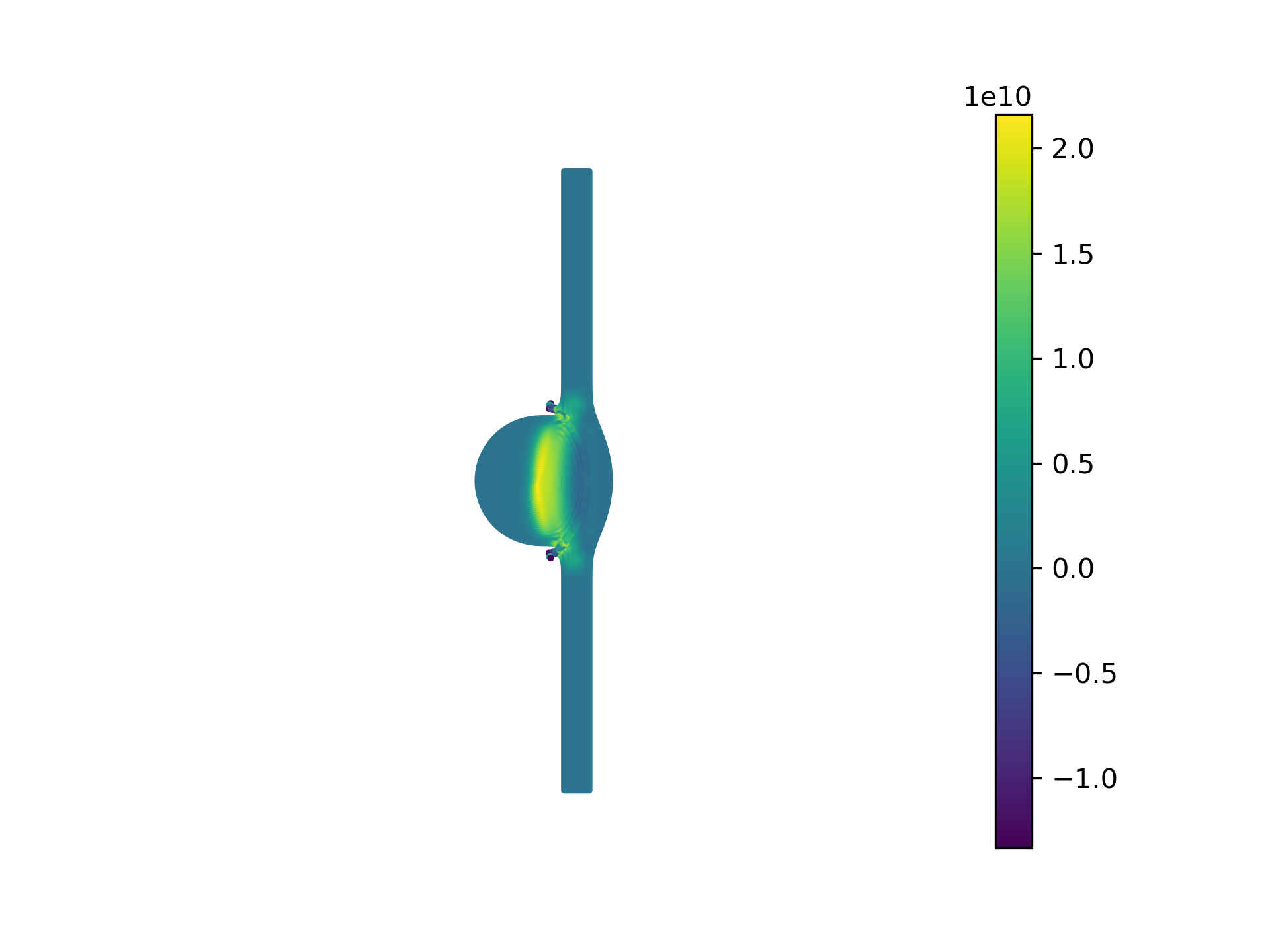
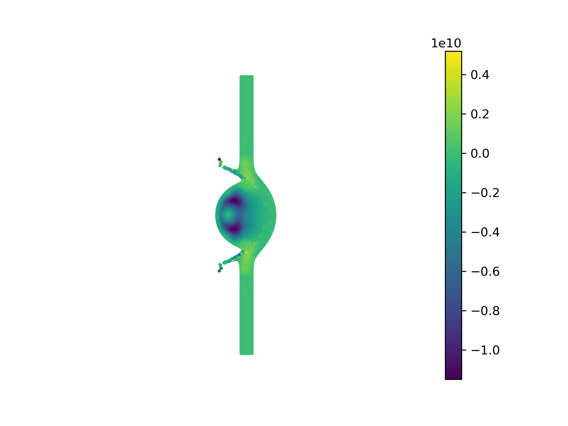
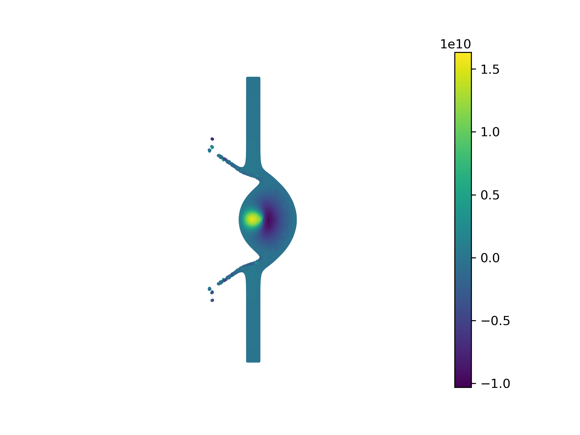
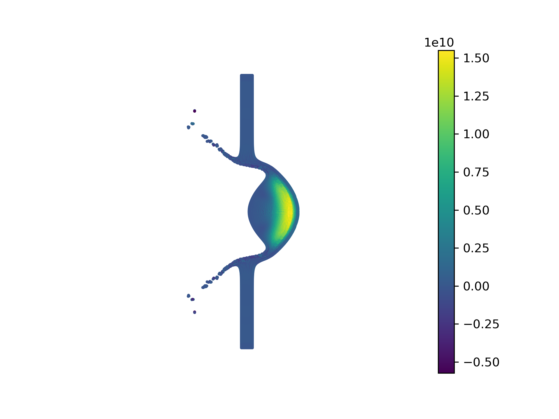
Figure 29 shows the plots of cylinder impacting the structure at different time instants. This is computed using the particle shifting technique of Sun [20]. The color contour represents the pressure of the particles. The width of the hole created by the cylinder is $19.6$ mm. When computed using the GTVF scheme [18] the hole has a size of $19.8$ mm. In Howell and Ball [40], the value cited is $19.2$ mm. We can see, that the current scheme is closer to the one simulated by [40], which is taken as reference in [18].

5 Discussion and conclusions

The proposed CTVF scheme builds on the original TVF scheme of Adami et al. [17] and is as an improvement on the GTVF of Zhang et al. [18]. In addition it generalizes the implementation of the EDAC-SPH method [21] where the TVF formulation was used for internal flows and a separate WCSPH formulation used for fluid flows with a free-surface. The current work proposes the addition of a few correction terms which improve the accuracy of the method as demonstrated in the earlier section. The addition of the terms imposes a small computational cost but compensates through the improved accuracy. As an example, in simulating the lid-driven cavity problem with a resolution of $50\times 50$, the original EDAC scheme without any of the correction terms with a one step predictor corrector integrator takes $251$ seconds for a time of $25$ seconds, the new scheme with a kick-drift-kick scheme takes $293$ seconds. Despite the change of the integrator this is a small increase in the performance. For solid mechanics problems we consider the colliding rings problem simulated for a total time of $0.016$ seconds. This takes $98$ seconds of time to simulate with the full CTVF scheme, and takes $73$ seconds without the corrections (run on Intel i5-7400, quad core machine). Free-surfaces are handled carefully. The method produces smoother pressure fields due to the use of the EDAC scheme. Finally the method is robust to changes in the PST method used. This has been demonstrated using both the PST of Sun et al. [20] and the IPST of Huang et al. [15].

An important feature of the proposed scheme is that it works well in the context of both fluid mechanics and solid mechanics. For elastic dynamics we propose correction terms that improve the accuracy and robustness of the method. The GTVF [18] method fails when the PST method is changed as demonstrated in section 4.4, however the proposed method is more robust. Furthermore, our method uses the true velocity in order to compute the velocity gradient. The results of the uniaxial compression problem in section 4.5 suggest that that the proposed method is more accurate than the GTVF. The main difference between the GTVF and the current scheme in the context of solid mechanics is the addition of the correction terms to the continuity equation, the usage of momentum velocity $\mathbf{u}$ in the computation of the velocity gradient, and the new particle shifting technique incorporation. We have found that the additional terms arising in the equation for the Jaumann stress rate eq. 4 has negligible influence and can be safely ignored. However, the computations in this work have included this term. The additional stress term in the momentum equation is negligible and has not been employed. We reiterate that for the fluid mechanics simulations the additional stress terms in the momentum equation are not negligible.

We note that for solid mechanics problems the method works well with either the traditional state equation used for the pressure evolution or the use of the EDAC equation. This does not make a significant difference for these problems since there is no additional damping added to the evolution equation for the deviatoric stresses. The EDAC evolution equation does make a significant improvement to the pressure evolution in the fluid mechanics problems as discussed earlier in [21].

The newly proposed method has not been applied to three dimensional problems or to fluid structure interaction (FSI) problems. We believe that the method would be easier to use in the context of FSI since it can handle both fluids and solids in the same formulation. We propose to investigate these in the future.

References

- Lucy [1977] Lucy, L.B.. A numerical approach to testing the fission hypothesis. The Astronomical Journal 1977;82(12):1013–1024.
- Gingold and Monaghan [1977] Gingold, R.A., Monaghan, J.J.. Smoothed particle hydrodynamics: Theory and application to non-spherical stars. Monthly Notices of the Royal Astronomical Society 1977;181:375–389.
- Monaghan [2005] Monaghan, J.J.. Smoothed Particle Hydrodynamics. Reports on Progress in Physics 2005;68:1703–1759.
- Monaghan [1994] Monaghan, J.J.. Simulating free surface flows with SPH. Journal of Computational Physics 1994;110:399–406.
- Cummins and Rudman [1999] Cummins, S.J., Rudman, M.. An SPH projection method. Journal of Computational Physics 1999;152:584–607.
- Randles and Libersky [1996] Randles, P., Libersky, L.. Smoothed Particle Hydrodynamics: Some recent improvements and applications. Computer Methods in Applied Mechanics and Engineering 1996;139(1-4):375–408. doi:10.1016/S0045-7825(96)01090-0.
- Gray et al. [2001] Gray, J., Monaghan, J., Swift, R.. SPH elastic dynamics. Computer Methods in Applied Mechanics and Engineering 2001;190(49-50):6641–6662. doi:10.1016/S0045-7825(01)00254-7; iSBN: 6139905443.
- Rafiee and Thiagarajan [2009] Rafiee, A., Thiagarajan, K.P.. An SPH projection method for simulating fluid-hypoelastic struc ture interaction. Computer Methods in Applied Mechanics and Engineering 2009;198(33):2785–2795. doi:10.1016/j.cma.2009.04.001.
- Khayyer et al. [2018] Khayyer, A., Gotoh, H., Falahaty, H., Shimi zu, Y.. An enhanced ISPH–SPH coupled method for simulation of incompr essible fluid–elastic structure interactions. Computer Physics Communications 2018;232:139–164. doi:10.1016/j.cpc.2018.05.012.
- Sun et al. [2021] Sun, P.N., Le Touzé, D., Oger, G., Zhang, A.M.. An accurate fsi-sph modeling of challenging fluid-structure interaction problems in two and three dimensions. Ocean Engineering 2021;221:108552. doi:10.1016/j.oceaneng.2020.108552.
- Bui et al. [2008] Bui, H.H., Fukagawa, R., Sako, K., Ohno, S.. Lagrangian meshfree particles method (sph) for large deformation and failure flows of geomaterial using elastic–plastic soil constitutive model. International Journal for Numerical and Analytical Methods in Geomechanics 2008;32(12):1537–1570. doi:https://doi.org/10.1002/nag.688.
- Xu et al. [2009a] Xu, R., Stansby, P., Laurence, D.. Accuracy and stability in incompressible sph (ISPH) based on the projection method and a new approach. Journal of Computational Physics 2009a;228(18):6703–6725. doi:10.1016/j.jcp.2009.05.032.
- Lind et al. [2012] Lind, S., Xu, R., Stansby, P., Rogers, B.. Incompressible smoothed particle hydrodynamics for free-surface flows: A generalised diffusion-based algorithm for stability and validations for impulsive flows and propagating waves. Journal of Computational Physics 2012;231(4):1499 – 1523. doi:10.1016/j.jcp.2011.10.027.
- Skillen et al. [2013] Skillen, A., Lind, S., Stansby, P.K., Rogers, B.D.. Incompressible smoothed particle hydrodynamics (sph) with reduced temporal noise and generalised fickian smoothing applied to body–water slam and efficient wave–body interaction. Computer Methods in Applied Mechanics and Engineering 2013;265:163 – 173. doi:10.1016/j.cma.2013.05.017.
- Huang et al. [2019] Huang, C., Long, T., Li, S., Liu, M.. A kernel gradient-free SPH method with iterative particle shifting technology for modeling low-Reynolds flows around airfoils. Engineering Analysis with Boundary Elements 2019;106:571–587. doi:10.1016/j.enganabound.2019.06.010.
- Ye et al. [2019] Ye, T., Pan, D., Huang, C., Liu, M.. Smoothed particle hydrodynamics (SPH) for complex fluid flows: Recent d evelopments in methodology and applications. Physics of Fluids 2019;31(1):011301.
- Adami et al. [2013] Adami, S., Hu, X., Adams, N.. A transport-velocity formulation for smoothed particle hydrodynamics. Journal of Computational Physics 2013;241:292–307. doi:10.1016/j.jcp.2013.01.043.
- Zhang et al. [2017] Zhang, C., Hu, X.Y.T., Adams, N.A.. A generalized transport-velocity formulation for smoothed particle hydrodynamics. Journal of Computational Physics 2017;337:216–232.
- Oger et al. [2016] Oger, G., Marrone, S., Le Touzé, D., de Leffe, M.. SPH accuracy improvement through the combination of a quasi-Lagrangian shifting transport velocity and consistent ALE formalisms. Journal of Computational Physics 2016;313:76–98. doi:10.1016/j.jcp.2016.02.039.
- Sun et al. [2019] Sun, P., Colagrossi, A., Marrone, S., Antuono, M., Zhang, A.M.. A consistent approach to particle shifting in the delta - Plus -SPH model. Computer Methods in Applied Mechanics and Engineering 2019;348:912–934. doi:10.1016/j.cma.2019.01.045.
- Ramachandran and Puri [2019] Ramachandran, P., Puri, K.. Entropically damped artificial compressibility for SPH. Computers and Fluids 2019;179(30):579–594. doi:10.1016/j.compfluid.2018.11.023.
- Clausen [2013] Clausen, J.R.. Entropically damped form of artificial compressibility for explicit simulation of incompressible flow. Physical Review E 2013;87(1):013309–1–013309–12. doi:10.1103/PhysRevE.87.013309.
- Antuono et al. [2021] Antuono, M., Sun, P., Marrone, S., Colagrossi, A.. The -ale-sph model: An arbitrary lagrangian-eulerian framework for the -sph model with particle shifting technique. Computers & Fluids 2021;216:104806.
- Ramachandran [2016] Ramachandran, P.. PySPH: a reproducible and high-performance framework for smoothed particle hydrodynamics. In: Benthall, S., Rostrup, S., eds. Proceedings of the 15th Python in Science Conference. 2016:127 – 135.
- Ramachandran et al. [2020] Ramachandran, P., Bhosale, A., Puri, K., Negi, P., Muta, A., Adepu, D., Menon, D., Govind, R., Sanka, S., Sebastian, A.S., Sen, A., Kaushik, R., Kumar, A., Kurapati, V., Patil, M., Tavker, D., Pandey, P., Kaushik, C., Dutt, A., Agarwal, A.. PySPH: a Python-based framework for smoothed particle hydrodynamics. arXiv preprint arXiv:190904504 2020;URL: https://arxiv.org/abs/1909.04504.
- Ramachandran [2018] Ramachandran, P.. automan: A python-based automation framework for numerical computing. Computing in Science & Engineering 2018;20(5):81–97. doi:10.1109/MCSE.2018.05329818.
- Antuono et al. [2010] Antuono, M., Colagrossi, A., Marrone, S., Molteni, D.. Free-surface flows solved by means of SPH schemes with numerical diffusive terms. Computer Physics Communications 2010;181(3):532 – 549. doi:https://doi.org/10.1016/j.cpc.2009.11.002.
- Ramachandran and Puri [2015] Ramachandran, P., Puri, K.. Entropically damped artificial compressibility for SPH. In: Liu, G.R., Das, R., eds. Proceedings of the 6th International Conference on Computational Methods 5 conference; vol. 2. Auckland, New Zealand; 2015:Paper ID 1210. URL: http://www.sci-en-tech.com/ICCM2015/PDFs/1210-3216-1-PB.pdf.
- Morris et al. [1997] Morris, J.P., Fox, P.J., Zhu, Y.. Modeling low reynolds number incompressible flows using sph. Journal of computational physics 1997;136(1):214–226.
- Sun et al. [2017] Sun, P., Colagrossi, A., Marrone, S., Zhang, A.. The plus-sph model: Simple procedures for a further improvement of the sph scheme. Computer Methods in Applied Mechanics and Engineering 2017;315:25–49.
- Xu et al. [2009b] Xu, R., Stansby, P., Laurence, D.. Accuracy and stability in incompressible sph (isph) based on the projection method and a new approach. Journal of computational Physics 2009b;228(18):6703–6725.
- Marrone et al. [2010] Marrone, S., Colagrossi, A., Le Touzé, D., Graziani, G.. Fast free-surface detection and level-set function definition in SPH solvers. Journal of Computational Physics 2010;229(10):3652–3663. doi:10.1016/j.jcp.2010.01.019.
- Muta et al. [2020] Muta, A., Ramachandran, P., Negi, P.. An efficient, open source, iterative ISPH scheme. Computer Physics Communications 2020;255:107283. doi:10.1016/j.cpc.2020.107283.
- Adami et al. [2012] Adami, S., Hu, X., Adams, N.. A generalized wall boundary condition for smoothed particle hydrodynamics. Journal of Computational Physics 2012;231(21):7057–7075. doi:10.1016/j.jcp.2012.05.005.
- Ghia et al. [1982] Ghia, U., Ghia, K.N., Shin, C.T.. High-Re solutions for incompressible flow using the Navier-Stokes equations and a multigrid method. Journal of Computational Physics 1982;48:387–411.
- Koshizuka and Oka [1996] Koshizuka, S., Oka, Y.. Moving-particle semi-implicit method for fragmentation of incompressible fluid. Nuclear science and engineering 1996;123(3):421–434.
- Landau et al. [1960] Landau, L.D., Lifshitz, E.M., Sykes, J.B., Reid, W.H., Dill, E.H.. Theory of elasticity: Vol. 7 of course of theoretical physics. Physics Today 1960;13(7):44–46. doi:10.1063/1.3057037.
- Das and Cleary [2015] Das, R., Cleary, P.W.. Evaluation of accuracy and stability of the classical sph method under uniaxial compression. Journal of Scientific Computing 2015;64(3):858–897.
- Swegle et al. [1995] Swegle, J.W., Hicks, D.L., Attaway, S.W.. Smoothed particle hydrodynamics stability analysis. Journal of computational physics 1995;116(1):123–134.
- Howell and Ball [2002] Howell, B., Ball, G.. A free-lagrange augmented Godunov method for the simulation of elastic–plastic solids. Journal of Computational Physics 2002;175(1):128–167.