Assessment of a transient homogeneous reactor through in situ adaptive tabulation

Abstract

The development of computational models for the numerical simulation of chemically reacting flows operating in the turbulent regime requires the solution of partial differential equations that represent the balance of mass, linear momentum, chemical species, and energy. The chemical reactions of the model may involve detailed reaction mechanisms for the description of the physicochemical phenomena. One of the biggest challenges is the stiffness of the numerical simulation of these models and the nonlinear nature of species rate of reaction. This work presents a study of in situ adaptive tabulation (ISAT) technique, focusing on the accuracy, efficiency, and memory usage in the simulation of homogeneous stirred reactor models using simple and complex reaction mechanisms. The combustion of carbon monoxide with oxygen and methane with air mixtures are considered, using detailed reaction mechanisms with 4 and 53 species, 3 and 325 reactions respectively. The results of these simulations indicate that the developed implementation of ISAT technique has a absolute global error smaller than 1%. Moreover, ISAT technique provides gains, in terms of computational time, of up to 80% when compared to the direct integration of the full chemical kinetics. However, in terms of memory usage the present implementation of ISAT technique is found to be excessively demanding.

1 Introduction

Combustion is a physicochemical phenomena characterized by a sequence of chemical reactions (most of then exothermic) which converts fuel/oxidizer mixtures (fresh gases) into combustion products (burned gases). Due to the large amount of energy released in these exothermic reactions, the combustion process is widely used in the operation of industrial devices such as gas turbines, process furnaces, etc.

Design and optimization of devices which operate based on combustion processes is an important engineering task, which demands the development of computational models as predictive tools. Such computational models may require the solution of partial differential equations that represent the balance of mass, linear momentum, chemical species, and energy. These models may include a detailed kinetic mechanism for the description of physicochemical phenomena involved Sabel’nikov et al (1998); Figueira da Silva and Deshaies (2000); Pimentel et al (2002); Walter and Figueira da Silva (2006). Typically, such reaction mechanisms for mixtures of hydrocarbons with air involve tenths of species, hundreds of elementary reactions, and timescales that vary up to nine orders of magnitude Williams (1985); Orbegoso et al (2011a, b).

Concerning the numerical simulation of these models, the challenge is related to reaction rate of the chemical species, which is nonlinear and presents a strong dependence with reaction mechanism dimension. Therefore, numerical simulation of a model with a detailed reaction mechanism is computationally demanding, which justifies the development of techniques to reduce the associated computational cost.

Several techniques to reduce the computational cost of these models are available in the literature. Essentially, they may be split into two classes. The first class includes techniques that seek to reduce the dimension of reaction mechanisms, such as Quasi-Steady State Approximation Frank-Kamenetskii (1940), Rate-Controlled Constrained Equilibrium Keck (1990), Computational Singular Perturbation Lam and Goussis (1994), the reduction to Skeleton Mechanisms Law (2006), Intrinsic Low-Dimensional Manifold Maas and Pope (1992), Proper Orthogonal Decomposition Holmes et al (1998), and Invariant Constrained Equilibrium Edge Pre-image Curve Ren et al (2006). The second class includes techniques that seek efficient algorithms to solve complex models, such as Look-Up Table Chen et al (1995), Repro-Modeling Turányi (1994), Piece-Wise Reusable Implementation of Solution Mapping Tonse et al (1999), Artificial Neural Network Ihme et al (2009), and In Situ Adaptive Tabulation (ISAT) Pope (1997); Singer and Pope (2004); Liu and Pope (2005); Lu and Pope (2009).

A characterization of one type of transient homogeneous reactor, using simple and complex thermochemistry, is presented in this this work. The analysis explores the effects of mixing to residence time scale ratios as reactor controlling parameter. The ISAT technique is employed to reduce the computational time spent to approximate the solution of the equations that governs the evolution of reactive mixture in this transient reactor. This work also investigates accuracy, performance, and memory usage of the present ISAT technique implementation. The accuracy analysis uses local and global metrics to quantify the error incurred by ISAT compared with a reference solution and investigates the statistical seed influence on the results. The performance is investigated by comparing the computational time gain obtained by ISAT with respect to a standard numerical integration procedure. The memory usage analysis quantifies the amount of memory used by ISAT implementation.

This work is organized as follows: the transient reactor of interest, its governing equation as well the numerical scheme used are presented in the second section. The third section presents the basic theory of ISAT technique. The fourth section discusses about the reactor configurations studied and ISAT implementation issues. Finally, in the fifth section, the main conclusions are summarized and a path for a future work is suggested.

2 Transient homogeneous reactor model

2.1 The geometry of reactive systems

In the framework of the transported probability density function (PDF) models Pope (1985), a reactive flow may be described by an ensemble of stochastic particles, which mimic the behavior of the fluid system.

Consider a transient spatially homogeneous reactive mixture evolving adiabatically and at constant pressure in a continuous flow reactor. The thermodynamical state of a fluid particle in this reactor may be completely determined by the mass fraction $Y_{i}$, where $i=1,\cdots,n_{s}$, of the $n_{s}$ chemical species and the specific enthalpy $h$, which can be lumped in the composition vector defined as

$$\bm{\phi}=\left(h,Y_{1},\cdots,Y_{n_{s}}\right)^{\mathtt{T}},$$ (1)

where the superscript ^T denotes the transposition operation. One should note that, due to the invariance of the system number of atoms, which ensures the total conservation of the mass, the components of vector $\bm{\phi}$ are not linearly independent.

The composition vector of each particle in this flow reactor evolves according to

$$\mathinner{\dfrac{\operatorname{d\!}{}\bm{\phi}}{\operatorname{d\!}{t}}}=-\bm{\Gamma}(\bm{\phi},t)+\bm{S}(\bm{\phi},t),$$ (2)

where $t$ denotes the time, $\bm{\Gamma}$ is the rate of change due to mixing, and $\bm{S}$ is the rate of change associated with the chemical reactions. Integrating Eq.(2) from an initial time $t_{0}$ to a time $t$ one obtain the reaction mapping

$$\bm{R}(\bm{\phi}_{0},t)=\bm{\phi}_{0}-\int_{t_{0}}^{t}\bm{\Gamma}(\bm{\phi},t^{\prime})dt^{\prime}+\int_{t_{0}}^{t}\bm{S}(\bm{\phi},t^{\prime})dt^{\prime},$$ (3)

which is the solution of Eq.(2) starting from the initial composition $\bm{\phi}(t_{0})=\bm{\phi}_{0}$. The reaction mapping corresponds to a trajectory in composition space, which, for large values of $t$, tends to the equilibrium composition for the given enthalpy and mass fractions on $\bm{\phi}_{0}$. The composition space is the $(n_{s}+1)$–dimensional Euclidean space where the first direction is associated with the enthalpy and the remaining $n_{s}$ are related to the chemical species.

2.2 Pairwise mixing stirred reactor

The classical Partially Stirred Reactor (PaSR), used in Correa (1993); Sabel’nikov and Figueira da Silva (2002), describes $\bm{\Gamma}$ by the interaction by exchange with the mean (IEM) micromixing model Fox (2003), but, for the purpose of testing a thermochemistry reduction technique, it is desirable to employ a mixing model that leads to a composition region accessed during the solution process which is “wider” than that provided by the IEM model. A modified version of PaSR model called Pairwise Mixing Stirred Reactor (PMSR), Pope (1997), is designed to yield a much larger accessed region, and, hence, should provide a stringent test on the ability of ISAT technique to yield a reduction in computational time.

In the PMSR model the reactor consists of an even number $n_{p}$ of particles, initially arranged in pairs $(j_{1},j_{2})$ such that the particles $(1,2)$, $(3,4)$, $\cdots$, $(n_{p}-1,n_{p})$ are partners. Given a time step, $\Delta t$, for each discrete time $k\Delta t$, where $k$ is an integer, the model is characterized by three types of events: inflow, outflow, and pairing. The inflow and outflow events consist of randomly selecting $n_{in}=\textsl{ceil}\left(\frac{1}{2}n_{p}(\Delta t/\tau_{r})\right)$ pairs of particles, being $\tau_{r}$ the residence time within the reactor, and exchanging their thermodynamical properties by the properties of a prescribed inflow. The pairing event consists of randomly selecting for pairing a number of pairs of particles, different from the inflow particles, equal to $n_{pair}=\textsl{ceil}\left(\frac{1}{2}n_{p}(\Delta t/\tau_{p})\right)$, being $\tau_{p}$ the pairwise time. Then the chosen particles (inflow/outflow and paring) are randomly shuffled. Between these discrete times, the pairs of particles $(j_{1},j_{2})$ evolve according to

$$\mathinner{\dfrac{\operatorname{d\!}{}\bm{\phi}}{\operatorname{d\!}{t}}}^{(j_{1})}=-\frac{\bm{\phi}^{(j_{1})}-\bm{\phi}^{(j_{2})}}{\tau_{m}}+\bm{S}(\bm{\phi}^{(j_{1})},t),$$ (4)

$$\mathinner{\dfrac{\operatorname{d\!}{}\bm{\phi}}{\operatorname{d\!}{t}}}^{(j_{2})}=-\frac{\bm{\phi}^{(j_{2})}-\bm{\phi}^{(j_{1})}}{\tau_{m}}+\bm{S}(\bm{\phi}^{(j_{2})},t).$$ (5)

where $\tau_{m}$ is the mixing time.

2.3 Numerical Integration

An operator splitting technique Yang and Pope (1998) is employed to numerically integrate Eq.(2). The overall process of integration via operator splitting technique can be represented as

$$\bm{\phi}(t)\stackrel{{\scriptstyle mixing}}{{\longrightarrow}}\bm{\phi}_{mix}(t+\Delta t)\stackrel{{\scriptstyle reaction}}{{\longrightarrow}}\bm{\phi}(t+\Delta t),$$ (6)

where given an initial composition $\bm{\phi}_{0}$ and a time step $\Delta t$, the first fractional step integrates the pure mixing system,

$$\mathinner{\dfrac{\operatorname{d\!}{}\bm{\phi}}{\operatorname{d\!}{t}}}=-\bm{\Gamma}(\bm{\phi},t),$$ (7)

to obtain $\bm{\phi}^{(j)}_{mix}(t+\Delta t)$. Then, the pure chemical reaction system,

$$\mathinner{\dfrac{\operatorname{d\!}{}\bm{\phi}}{\operatorname{d\!}{t}}}=\bm{S}(\bm{\phi},t).$$ (8)

is integrated from an initial composition $\bm{\phi}_{mix}(t+\Delta t)$ over a time step $\Delta t$ and gives $\bm{\phi}(t+\Delta t)$.

The operator splitting technique allows to solve each term in the evolution equation, Eq.(2), separately, using specific efficient numerical methods to treat the particular features inherent to the physical phenomenon modeled by each term Fox (2003).

3 In situ adaptive tabulation

3.1 Linearized reaction mapping

Consider a composition $\bm{\phi}$ and an initial composition $\bm{\phi}_{0}$, so that Taylor expansion of the reaction mapping of $\bm{\phi}$ around $\bm{\phi}_{0}$ is

$$\bm{R}(\bm{\phi},t)=\bm{R}(\bm{\phi}_{0},t)+\bm{A}(\bm{\phi}_{0},t)\delta\bm{\phi}+\mathcal{O}(\mathinner{\!\left\lVert\delta\bm{\phi}\right\rVert}^{2}),$$ (9)

where $\delta\bm{\phi}=\bm{\phi}-\bm{\phi}_{0}$, $\bm{A}(\bm{\phi}_{0},t)$ is a $n_{\phi}\times n_{\phi}$ matrix, called mapping gradient matrix, with components given by

$$A_{ij}(\bm{\phi}_{0},t)=\mathinner{\dfrac{\partial{}R_{i}}{\partial{\phi_{0_{j}}}}}(\bm{\phi}_{0},t),$$ (10)

$\mathinner{\!\left\lVert\cdot\right\rVert}$ denotes the Euclidean norm of a vector, and $\mathcal{O}(\mathinner{\!\left\lVert\delta\bm{\phi}\right\rVert}^{2})$ denotes terms that have order $\mathinner{\!\left\lVert\delta\bm{\phi}\right\rVert}^{2}$.

The linear approximation $\bm{R}^{l}(\bm{\phi},t)$, obtained by neglecting the high order terms of Eq.(9), is second-order accurate at a connected region of composition space centered at $\bm{\phi}_{0}$. The shape of this region is unknown before the calculations, but ISAT algorithm approximates this region by a hyper-ellipsoid, as will be shown in section 3.2. The local error of this linear approximation is defined as the Euclidean norm of the difference between the reaction mapping at $\bm{\phi}$ and the linear approximation for it around $\bm{\phi}_{0}$,

$$\varepsilon=\mathinner{\!\left\lVert\bm{R}(\bm{\phi},t)-\bm{R}^{l}(\bm{\phi},t)\right\rVert}.$$ (11)

3.2 Ellipsoid of accuracy

The accuracy of the linear approximation at $\bm{\phi}_{0}$ is controlled only if the local error is smaller than a positive error tolerance $\varepsilon_{tol}$, which is heuristically chosen. The region of accuracy is defined as the connected region of the composition space centered at $\bm{\phi}_{0}$ where local error is not greater than $\varepsilon_{tol}$. As shown in Pope (1997), this region is approximated by a hyper-ellipsoid centered at $\bm{\phi}_{0}$ which is dubbed ellipsoid of accuracy (EOA), and is mathematically represented by the following inequation

$$\delta\bm{\phi}^{\mathtt{T}}\bm{L}\bm{L}^{\mathtt{T}}\delta\bm{\phi}\leq\varepsilon_{tol}^{2},$$ (12)

where the EOA Cholesky matrix, denoted by $\bm{L}$, is lower triangular Golub and Van Loan (1996).

The adaptive step of ISAT algorithm involves the solution of the following geometric problem: given a hyper-ellipsoid centered at $\bm{\phi}_{0}$ and a query composition, $\bm{\phi}_{q}$, outside it, determine a new hyper-ellipsoid of minimum hyper-volume, centered at $\bm{\phi}_{0}$, which encloses both the original hyper-ellipsoid and the point $\bm{\phi}_{q}$. The solution of this problem is presented by Pope (2008) and is not shown here for sake of brevity.

3.3 Tabulation procedure

Initially ISAT algorithm receives the time step $\Delta t$ and the tolerance $\varepsilon_{tol}$. Then, in every time step, ISAT algorithm receives a query composition $\bm{\phi}_{q}$ and returns an approximation for the corresponding reaction mapping $\bm{R}(\bm{\phi}_{q},t)$. This approximation is obtained via numerical integration of Eq.(8) or by the linear approximation $\bm{R}^{l}(\bm{\phi}_{q},t)$.

During the reactive flow calculation, the computed values are sequentially stored in a table for future use. This process is known as in situ tabulation. The ISAT table, which is created by the tabulation process, includes the initial composition $\bm{\phi}_{0}$, the reaction mapping $\bm{R}(\bm{\phi}_{0},t)$, and the mapping gradient matrix $\bm{A}(\bm{\phi}_{0},t)$. Using these elements it is possible to construct the linear approximation. As the calculation proceeds, a new query composition, $\bm{\phi}_{q}$, is received by ISAT and the table is transversed until a $\bm{\phi}_{0}$ is found that is close to $\bm{\phi}_{q}$. Depending on the accuracy, the linear approximation around $\bm{\phi}_{0}$ is returned or the reaction mapping of $\bm{\phi}_{q}$ is obtained by direct integration of Eq.(8).

The ISAT table is a binary search tree, since this data structure allows for searching an information in $\mathcal{O}(\log_{2}{n_{tab}})$ operations, where $n_{tab}$ is the total number entries in the tree, if the tree is balanced Knuth (1998). The binary search tree is basically formed by two types of elements, nodes, and leaves. Each leaf of the tree stores the following data:

• $\bm{\phi}_{0}$: initial composition;

• $\bm{R}(\bm{\phi}_{0},t)$: reaction mapping at $\bm{\phi}_{0}$;

• $\bm{A}(\bm{\phi}_{0},t)$: mapping gradient matrix at $\bm{\phi}_{0}$;

• $\bm{L}$: EOA Cholesky matrix.

Each node of the binary search tree has an associated cutting plane. This plane is defined by a normal vector

$$\bm{v}=\bm{\phi}_{q}-\bm{\phi}_{0},$$ (13)

and a scalar

$$a=\bm{v}^{\mathtt{T}}\left(\frac{\bm{\phi}_{q}+\bm{\phi}_{0}}{2}\right),$$ (14)

such that all compositions $\bm{\phi}$ with $\bm{v}^{T}\bm{\phi}>a$ are located to the “right" of the cutting plane, as sketched in Figure 1. The cutting plane construction defines a search criterion in the binary search tree.

Figure 1: Cutting plane in relation to EOA position.

If during the calculation a query point $\bm{\phi}_{q}$ is encountered within the region of accuracy, i.e., $\varepsilon\leq\varepsilon_{tol}$, but outside the estimate of EOA, then the EOA growth proceeds as detailed in Pope (2008). The first three items stored in the binary search tree leaf $\left[\bm{\phi}_{0},\leavevmode\nobreak\ \bm{R}(\bm{\phi}_{0},t)\leavevmode\nobreak\ \mbox{and}\leavevmode\nobreak\ \bm{A}(\bm{\phi}_{0},t)\right]$ are computed once, whereas $\bm{L}$ changes whenever the EOA is grown.

Once a query composition $\bm{\phi}_{q}$ is received by ISAT table, the binary search tree is initialized as a single leaf and the exact value of the reaction mapping is returned.

The subsequent steps are:

1. Given a query composition the tree is transversed until a leaf ($\bm{\phi}_{0}$) is found.

2. Equation (12) is used to determine if $\bm{\phi}_{q}$ is inside EOA or not.

3. If $\bm{\phi}_{q}$ is inside EOA, the reaction mapping is given by the linear approximation. This is the first of four outcomes, called retrieve.

4. If $\bm{\phi}_{q}$ is outside EOA, direct integration is used to compute the reaction mapping, and the local error is measured by Eq.(11).

5. If the local error is smaller than tolerance, $\varepsilon_{tol}$, the EOA is grown according to the procedure presented in Pope (2008) and the reaction mapping is returned. This outcome is called growth.

6. If local error is greater than the tolerance $\varepsilon_{tol}$ and the maximum number of entries in the binary search tree is not reached, a new record is stored in the binary search tree based on $\bm{\phi}_{q}$ and the reaction mapping is returned. The original leaf is replaced by a node with the left leaf representing the old composition $\bm{\phi}_{0}$ and the right leaf the new one $\bm{\phi}_{q}$ as shown in Figure 2. This outcome is an addition.

7. If the local error is greater than the tolerance $\varepsilon_{tol}$ and the maximum number of entries in the binary search tree is reacted, the reaction mapping is returned. This outcome is called direct evaluation.

Figure 2: Binary search tree before and after the addition of a new node.

4 Results and discussion

This section presents the results of numerical simulations performed in order to assess characteristics of PMSR reactor. This study investigates three configurations of a PMSR reactor, two mixtures of $CO/O_{2}$, and one mixture of $CH_{4}$/air, using different time scales to define their behavior. Accuracy, performance, and memory usage of ISAT technique implementation are also investigated. For this purpose, the approximation for solution of the model equation, Eq.(2), obtained by ISAT technique are compared with a reference solution from direct integration (DI) procedure, described in section 2.3.

4.1 $CO/O_{2}$ mixture

The first two cases studied consider a 1024 particles PMSR, initially filled with a fuel-lean mixture of $CO/O_{2}$ at $2948.5\leavevmode\nobreak\ \mathrm{K}$ and $1\leavevmode\nobreak\ \mathrm{atm}$. At every time step, a fuel-lean mixture of $CO/O_{2}$ enters the reactor at $T_{in}=300\leavevmode\nobreak\ \mathrm{K}$ and $p_{in}=1\leavevmode\nobreak\ \mathrm{atm}$. Both fuel-leam mixtures have equivalence ratio equal to $0.7$. The constant pressure and enthalpy equilibrium state associated to the inflow mixture is reached at $T_{eq}=2948.5\leavevmode\nobreak\ \mathrm{K}$. The reaction mechanism used to describe $CO$ with $O_{2}$ kinetics involves 4 species and 3 reactions, Gardiner (2000). For the first case a time scales configuration with $\tau_{m}/\tau_{r}=\tau_{p}/\tau_{r}=1/2$ is used, so that the pairwise/mixing time scales are of the same order of magnitude as the residence time. In this situation, partially stirred reactor (PaSR) conditions result within the reactor. For the second case, time scales configuration adopted is $\tau_{m}/\tau_{r}=\tau_{p}/\tau_{r}=1/10$, so that the pairwise/mixing time scales are small when compared to the residence time. Thus, the reactor should behave almost as a perfect stirred reactor (PSR), where the processes of mixing and pairing occur instantaneously. These cases use a binary search tree with a maximum of $50,000$ entries, $\Delta t=10\leavevmode\nobreak\ \mathrm{\mu s}$, and $\varepsilon_{tol}=10^{-3}$.

4.2 $CH_{4}$/air mixture

The third case studied consists of a PMSR, with 1024 particles, initially filled with the combustion products of a stoichiometric mixture of $CH_{4}$/air at $2100\leavevmode\nobreak\ \mathrm{K}$ and $1\leavevmode\nobreak\ \mathrm{atm}$. At every time step, a stoichiometric mixture of $CH_{4}$/air enters the reactor at $T_{in}=300\leavevmode\nobreak\ \mathrm{K}$ and $p_{in}=1\leavevmode\nobreak\ \mathrm{atm}$. The constant pressure and enthalpy equilibrium state associated to this mixture is reached at $T_{eq}=2225.5\leavevmode\nobreak\ \mathrm{K}$. The reaction of $CH_{4}$ with air kinetics is described by GRI mechanism version 3.0 Smith et al (????), with 53 species and 325 reactions. For this PMSR one have $\tau_{m}/\tau_{r}=\tau_{p}/\tau_{r}=1/4$, so that it is expected to behave like a PaSR. This simulation uses a binary search tree with a maximum of 60,000 entries, $\Delta t=0.1\leavevmode\nobreak\ \mathrm{ms}$ and $\varepsilon_{tol}=10^{-3}$.

4.3 Analysis of reactor behavior

Figures 3 and 4 show the comparison between DI and ISAT calculations, as function of the dimensionless time $\tau^{\ast}=t/\tau_{r}$, for the ensemble average $\left\langle T\right\rangle^{\ast}$ and the ensemble variance $\left\langle T^{\prime 2}\right\rangle^{\ast}$ of the reduced temperature in the cases 1 and 2, where the reduced temperature is defined as

$$T^{\ast}=\frac{T-T_{in}}{T_{eq}-T_{in}},$$ (15)

and the ensemble average and the ensemble variance operators are respectively defined as

$$\left\langle\psi\right\rangle=\frac{1}{n_{p}}\sum_{j=1}^{n_{p}}\psi^{(j)}\qquad\mbox{and}\qquad\left\langle\psi^{\prime 2}\right\rangle=\left\langle\psi^{2}\right\rangle-\left\langle\psi\right\rangle^{2},$$ (16)

being $\psi$ a generic property of the reactive system.

For case 1 results, which span over a range of $500$ residence times, one can observe an excellent qualitative agreement for $\left\langle T\right\rangle^{\ast}$ and $\left\langle T^{\prime 2}\right\rangle^{\ast}$. The ensemble average value rapidly drops from the initial value to reach the statistically steady-state regime around $\left\langle T\right\rangle^{\ast}=0.3$. The ensemble variance rapidly grows, then decreases until it reaches the statistically steady-state value around $\left\langle T^{\prime 2}\right\rangle^{\ast}=0.13$. The analysis of the two figures shows that the statistically steady-state regime is reached after $\tau^{\ast}=10$.

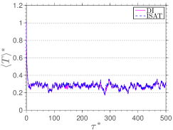
(a) Evolution of $\left\langle T\right\rangle^{\ast}$ for case 1.

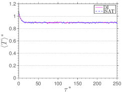
(b) Evolution of $\left\langle T\right\rangle^{\ast}$ for case 2.

Figure 3: Comparison between DI (—) and ISAT (- - -) calculations of the ensemble average of the reduced temperature.

In case 2, where a range of $250$ residence times have been computed, one can also observe an excellent qualitative agreement for $\left\langle T\right\rangle^{\ast}$ and $\left\langle T^{\prime 2}\right\rangle^{\ast}$. Again, the overall history of the PMSR is the same for DI and ISAT. Similar results, not shown here for sake of brevity, have been obtained for the other thermochemical properties of the reactors.

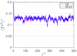
(a) Evolution of $\left\langle T^{\prime 2}\right\rangle^{\ast}$ for case 1.

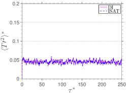
(b) Evolution of $\left\langle T^{\prime 2}\right\rangle^{\ast}$ for case 2.

Figure 4: Comparison between DI (—) and ISAT (- - -) calculations of the ensemble variance of the reduced temperature.

The difference among both cases is due to the behavior of each reactor at the statistically steady state regime. Indeed, the case 2 reactor behavior is governed by a competition between the chemical and residence times mostly. Therefore, the thermodynamical properties steady-state PDF is concentrated over a smaller range than in case 1, where the mixing and pairing time scales are large when compared to the residence time. This behavior is illustrated in Figures 5 and 6, which present the comparison between DI and ISAT computations of mean histograms, averaged over the last $50$ residence times, of $T^{\ast}$ and $Y_{O}$ for cases 1 and 2. These figures underscore the influence of PMSR controlling parameters, i.e., the time scales ratios $\tau_{m}/\tau_{r}$ and $\tau_{p}/\tau_{r}$, on the thermochemical conditions prevailing within each reactor. Indeed, the temperature within the case 2 reactor is such that almost only burned gases are found. On the other hand, case 1 reactor is characterized by a bimodal temperature distribution with a large probability of finding $T^{\ast}=0.04$ and a broader temperature distribution leaning toward the burned gases. Such a distribution, as it could be expected, is reflected on $Y_{O}$ histogram, which also exhibits a bimodal distribution.

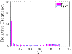
(a) Histogram of $T^{\ast}$ for case 1.

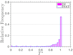
(b) Histogram of $T^{\ast}$ for case 2.

Figure 5: Comparison between DI and ISAT calculations of the mean histograms (averaged over the last $50$ residence times) of the reduced temperature.

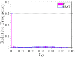
(a) Histogram of $Y_{O}$ for case 1.

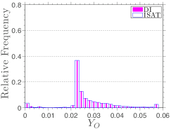
(b) Histogram of $Y_{O}$ for case 2.

Figure 6: Comparison between DI and ISAT calculations of the mean histograms (averaged over the last $50$ residence times) of the $O$ mass fraction.

The comparison between DI and ISAT results for the first two statistical moments of $T^{\ast}$ and $Y_{OH}$, for case 3, are presented in Figures 7 and 8. One can note reasonable and good agreements for the $T^{\ast}$ and the $Y_{OH}$ statistics, respectively. The results of case 3 show a large discrepancy for the $T^{\ast}$ than that obtained in case 1. The reaction mechanism of methane is much more complex than the mechanism used to model the carbon monoxide chemical kinetics in case 1, which would in principle lead to the PMSR with methane to assume a wider range of possible thermodynamic states. Thus, it could be expected that the present binary search tree, with $60\mathrm{k}$ entries (almost similar to that used in case 1), would yield comparatively lower accuracy.

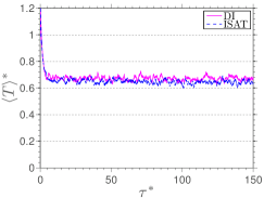
(a) Evolution of $\left\langle T\right\rangle^{\ast}$ for case 3.

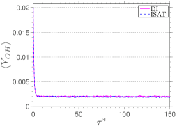
(b) Evolution of $\left\langle Y_{OH}\right\rangle$ for case 3.

Figure 7: Comparison between DI (—) and ISAT (- - -) calculations of the ensemble average of the reduced temperature and $OH$ mass fraction.

(a) Evolution of $\left\langle T^{\prime 2}\right\rangle^{\ast}$ for case 3.

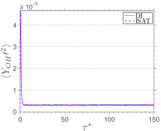
(b) Evolution of $\left\langle Y_{OH}^{\prime 2}\right\rangle$ for case 3.

Figure 8: Comparison between DI (—) and ISAT (- - -) calculations of the ensemble variance of the reduced temperature and $OH$ mass fraction.

Finally, Figure 9 presents the comparison between DI and ISAT computations of the mean histograms, averaged over the last $50$ residence times, of the $T^{\ast}$ and $Y_{HCO}$ for case 3. The temperature histogram presents a bimodal distribution with large probability of finding $T^{\ast}\geq 0.9$ and a broader temperature distribution leaning to the fresh gases. On the other hand, $Y_{HCO}$ histogram shows a distribution essentially concentrated in the fresh gases region, and nearly homogeneous elsewhere. This behavior illustrates the fact that $HCO$, an intermediate species, appears in low concentration in the burned gases.

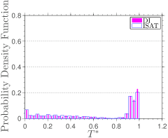
(a) Histogram of $T^{\ast}$ for case 3.

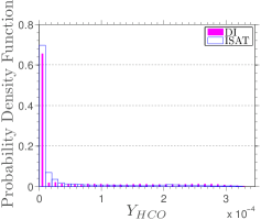
(b) Histogram of $Y_{HCO}$ for case 3.

Figure 9: Comparison between DI and ISAT computations of the mean histograms (averaged over the last $50$ residence times) of the reduced temperature and $HCO$ mass fraction.

4.4 Analysis of ISAT accuracy

The relative local error of $\psi$, which is a time dependent function, is defined as

$$\varepsilon_{{}_{r},\psi}(t)=\Big{|}\frac{\psi_{DI}(t)-\psi_{ISAT}(t)}{\psi_{DI}(t)}\Big{|},$$ (17)

where subscripts _DI and _ISAT denote DI and ISAT calculations of $\psi$, respectively. This metric represents a local measure of error incurred by ISAT.

The evolution of the relative local errors of $T^{\ast}$ and $Y_{O}$ statistical moments are presented in Figures 10 and 11. Concerning case 1 errors, one can observe a large statistical variation due to the stochastic nature of the PMSR model, with amplitudes reaching 13%. In case 2, relative errors of the order of 1% only can be observed.

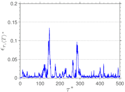
(a) Evolution of $\varepsilon_{{}_{r},\left\langle T\right\rangle^{\ast}}$ for case 1

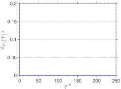
(b) Evolution of $\varepsilon_{{}_{r},\left\langle T\right\rangle^{\ast}}$ for case 2

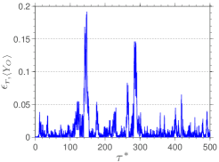
(c) Evolution of $\varepsilon_{{}_{r},\left\langle Y_{O}\right\rangle}$ for case 1

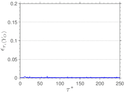
(d) Evolution of $\varepsilon_{{}_{r},\left\langle Y_{O}\right\rangle}$ for case 2

Figure 10: Evolution of the relative local error for the ensemble average of the reduced temperature and of the $O$ mass fraction, using the same statistical seeds in both cases.

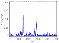
(a) Evolution of $\varepsilon_{{}_{r},\left\langle T^{\prime 2}\right\rangle^{\ast}}$ for case 1

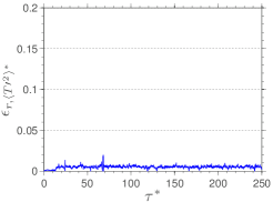
(b) Evolution of $\varepsilon_{{}_{r},\left\langle T^{\prime 2}\right\rangle^{\ast}}$ for case 2

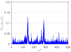
(c) Evolution of $\varepsilon_{{}_{r},\left\langle Y_{O}^{\prime 2}\right\rangle}$ for case 1

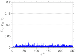
(d) Evolution of $\varepsilon_{{}_{r},\left\langle Y_{O}^{\prime 2}\right\rangle}$ for case 2

Figure 11: Evolution of the relative local error for the ensemble variance of the reduced temperature and of the $O$ mass fraction, using the same statistical seeds in both cases.

All realizations of the stochastic processes in DI and ISAT calculations shown above use the same statistical seed for pseudorandom number generator. However, since the mixing model is statistical in nature, it could be expected that the seed value may influence the ISAT behavior. Therefore, if the DI calculation seed is kept fixed and ISAT seed is changed, the results for $\left\langle T\right\rangle^{\ast}$ and $\varepsilon_{{}_{r},\left\langle T\right\rangle^{\ast}}$ are expected to be modified. This can be seen in Figure 12, where one may observe, by comparison with Figures 3 and 10, an increase in the $\varepsilon_{{}_{r},\left\langle T\right\rangle^{\ast}}$ for both cases.

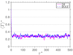
(a) Evolution of $\left\langle T\right\rangle^{\ast}$ for case 1.

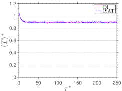
(b) Evolution of $\left\langle T\right\rangle^{\ast}$ for case 2.

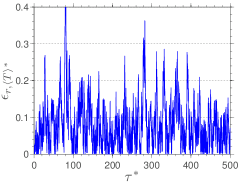
(c) Evolution of $\varepsilon_{{}_{r},\left\langle T\right\rangle^{\ast}}$ for case 1

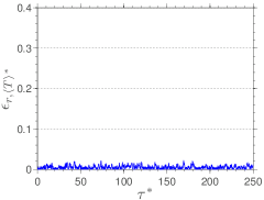
(d) Evolution of $\varepsilon_{{}_{r},\left\langle T\right\rangle^{\ast}}$ for case 2

Figure 12: Comparison between DI (—) and ISAT (- - -) calculations, using different statistical seeds, of the ensemble average of the reduced temperature and the corresponding relative local errors.

The analysis of the graphs in Figure 12 indicates that 1024 particles are not sufficient to guarantee the statistical independence of the computed results. This hypothesis is also confirmed if one considers Figure 13, where it is possible to see discrepancies in DI and ISAT mean histograms of $T^{\ast}$ for both cases, even if, qualitatively these histograms are not much different than those shown in Figure 5. Thus, one can conclude that although the results not exhibit the statistical independence with a sample of 1024 particles, they do not vary much with a sample of this size. Possibly a sample of 4096 particles is sufficient to ensure the independence of the results.

(a) Histogram of $T^{\ast}$ for case 1.

(b) Histogram of $T^{\ast}$ for case 2.

Figure 13: Comparison between DI and ISAT calculations, using different statistical seeds, of the mean histograms (averaged over the last $50$ residence times) of the reduced temperature.

The mean relative error of $\psi$ over an interval $\Delta\tau$, defined as

$$\left\langle\varepsilon_{{}_{r},\psi}\right\rangle_{M}=\frac{1}{\Delta\tau}\int_{t}^{t+\Delta\tau}\varepsilon_{{}_{r},\psi}(t^{\prime})dt^{\prime},$$ (18)

is a metric that gives a global measure of the error incurred by ISAT.

The mean relative errors associated to the statistical moments of the $T^{\ast}$ and the $Y_{O}$ are presented in Table 1. One can observe that, when the same seed is used for ISAT and DI, the mean error of the average properties is smaller than 1.2% in case 1, and of 0.1% in case 2 only. For $T^{\ast}$ and $Y_{O}$ ensemble variances, the mean error is large in case 1. Concerning the simulations where the used seeds are different, the mean error of the properties average/variance are an order of magnitude greater than the previous one.

Table 1: Mean relative error of $\psi$ for cases 1 and 2.

	Equal Seeds		Different Seeds
$\psi$	Case 1	Case 2	Case 1	Case 2
$\left\langle T\right\rangle^{\ast}$	$\leavevmode\nobreak\ 1.0\leavevmode\nobreak\ \%$	$\leavevmode\nobreak\ 0.0\leavevmode\nobreak\ \%$	8.1 %	5.3 %
$\left\langle Y_{O}\right\rangle$	$\leavevmode\nobreak\ 1.2\leavevmode\nobreak\ \%$	$\leavevmode\nobreak\ 0.1\leavevmode\nobreak\ \%$	11.7 %	1.3 %
$\left\langle T^{\prime 2}\right\rangle^{\ast}$	$\leavevmode\nobreak\ 1.0\leavevmode\nobreak\ \%$	$\leavevmode\nobreak\ 0.5\leavevmode\nobreak\ \%$	6.6 %	10.1 %
$\left\langle Y_{O}^{\prime 2}\right\rangle$	$\leavevmode\nobreak\ 0.9\leavevmode\nobreak\ \%$	$\leavevmode\nobreak\ 0.5\leavevmode\nobreak\ \%$	7.0 %	6.1 %

In the early development of ISAT technique Pope (1997) it was noted that the choice of the tolerance could affect the accuracy of the problem solution. In order to investigate the effect of the tolerance on the present results, Figure 14 presents the absolute global error, $\varepsilon_{g}$, as a function of ISAT error tolerance for cases 1 and 2. The absolute global error is defined, over a time interval $\Delta\tau$, as

$$\varepsilon_{g}=\frac{1}{\Delta\tau}\int_{t}^{t+\Delta\tau}\mathinner{\!\left\lVert\left\langle\bm{\phi}\right\rangle(t^{\prime})_{DI}-\left\langle\bm{\phi}\right\rangle(t^{\prime})_{ISAT}\right\rVert}\leavevmode\nobreak\ dt^{\prime},$$ (19)

where $\left\langle\bm{\phi}\right\rangle$ denotes a vector which the components are the ensemble averages of $\bm{\phi}$ components.

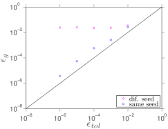
(a) $\varepsilon_{g}$ vs $\varepsilon_{tol}$ for case 1.

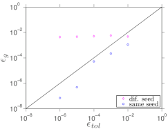
(b) $\varepsilon_{g}$ vs $\varepsilon_{tol}$ for case 2.

Figure 14: Absolute global errors as function of the error tolerance, using a binary search tree with $50\mathrm{k}$ entries.

As may be seen in Figure 14, when the same statistical seed is used, $\varepsilon_{g}$ decreases linearly as $\varepsilon_{tol}$ is reduced, for both studied cases. However, if different statistical seeds are used, one can note a limit behavior where $\varepsilon_{g}$ does not decrease if $\varepsilon_{tol}$ is reduced. This saturation in $\varepsilon_{g}$ value ($\sim 10^{-2}$) indicates that a decrease in $\varepsilon_{tol}$ value below $10^{-3}$ is not effective in cases where the statistical seeds are different.

The evolution of the relative local error of the statistical moments of $T^{\ast}$ and $Y_{OH}$, for case 3, are presented in Figure 15. Compared with the results of case 1, the errors of case 3 present more oscillations. Furthermore, for this case, $\varepsilon_{g}=2.4\times 10^{-3}$ is an order of magnitude larger than the values obtained in cases 1 and 2, also using $\varepsilon_{tol}=10^{-3}$. Since different seeds are used for DI and ISAT calculations in case 3, large errors in the results are to be expected.

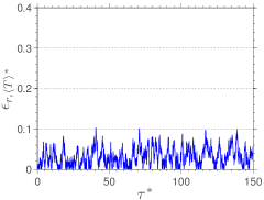
(a) Evolution of $\varepsilon_{{}_{r},\left\langle T\right\rangle^{\ast}}$ for case 3.

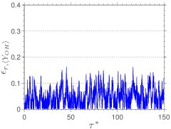
(b) Evolution of $\varepsilon_{{}_{r},\left\langle Y_{OH}\right\rangle}$ for case 3.

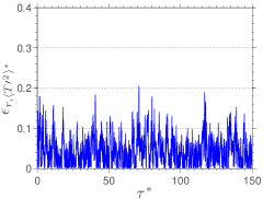
(c) Evolution of $\varepsilon_{{}_{r},\left\langle T^{\prime 2}\right\rangle^{\ast}}$ for case 3.

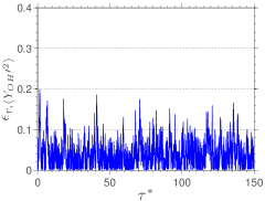
(d) Evolution of $\varepsilon_{{}_{r},\left\langle Y_{OH}^{\prime 2}\right\rangle}$ for case 3.

Figure 15: Evolution of the relative local error of the ensemble average mean and the ensemble average variance of the reduced temperature and $OH$ mass fraction.

4.5 Analysis of ISAT performance

The comparison of time evolution of ISAT outputs (number of additions, growths, retrieves, and direct evaluations) and of binary search tree height, as well as the corresponding rates of change, for cases 1 and 2, are presented in Figures 16 and 17. A first important observation is that the number of additions in both cases reaches the maximum prescribed value in the binary search tree of $50\mathrm{k}$. As a consequence of binary search tree saturation, the additions curve reaches a steady state after $5.4$ and $1.2$ residence times ($\tau_{r}$), in the first and second cases, respectively. This indicates that ISAT table is saturated earlier when mixing is faster ($\tau_{m}/\tau_{r}$ small).

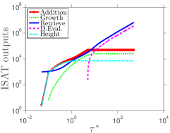
(a) Case 1.

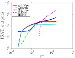
(b) Case 2.

Figure 16: Evolution of ISAT algorithm outputs and of the height of ISAT binary search tree.

Figures 16 and 17 also show the evolution of binary tree height, which reaches steady state $1.8\leavevmode\nobreak\ \tau_{r}$ in the first case and $0.4\leavevmode\nobreak\ \tau_{r}$ in the second case. It is also noteworthy that, in both cases, the tree height is an order of magnitude smaller than the total number of entries in the tree ($\sim 17\mathrm{k}$ in case 1 and $\sim 7\mathrm{k}$ in case 2). This difference between height and total entries in data table ensures the efficiency of search process for a new query, which could be performed up to three and seven times faster in cases 1 and 2, respectively, than a vector search.

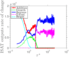
(a) Case 1.

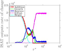
(b) Case 2.

Figure 17: Evolution of the rates of change of each ISAT algorithm outputs and of the height of ISAT binary search tree.

In the first case, Figures 16 and 17 show that the number of growths presents a sharp rate of change around $\tau_{r}$, whereas, in the second case, this occurs around $5\leavevmode\nobreak\ \tau_{r}$. In both cases, growth steady state occurs after $10\leavevmode\nobreak\ \tau_{r}$. During both simulations the number of growths is always smaller than additions. This indicates that the desirable massive increase of the ellipsoids of accuracy, to improve the estimate of the region of accuracy, is not observed. This behavior might circumstantial to the reaction system of the carbon monoxide considered, since, due to its simplicity (only three reactions), a small part of the realizable region should be assessed during the course of the calculation.

The Figure 16 shows that, after tree saturation occurs, the number of retrieves, and direct evaluations exceed the number of additions in both cases. In case 1 there is a higher occurrence of retrieve events, whereas in case 2 direct evaluations prevail. The number of retrieves exhibits a linear limit behavior in both cases. The ISAT behavior for the second case reflects the fact that the binary tree of this case is poor, i.e., contains too few compositions in the region accessed by the calculation. As a consequence, the number of direct evaluations vastly outnumbers ISAT operations. This explains the error behavior observed in section 4.4.

When ISAT technique is more efficient than DI procedure, the computational time spent by ISAT is smaller than computational time spent by DI. The computational time spent by ISAT is the sum of the computational time spent at each of its possible outputs. Therefore, the efficiency condition can be stated as

$$n_{A}\tau_{A}+n_{G}\tau_{G}+n_{R}\tau_{R}+n_{DE}\tau_{DE}<n_{DI}\tau_{DI},$$ (20)

where $n_{A}$, $n_{G}$, $n_{R}$, $n_{DE}$, $n_{DI}$ are the number of additions, growths, retrieves, direct evaluations, and direct integrations, respectively, whereas $\tau_{A}$, $\tau_{G}$, $\tau_{R}$, $\tau_{DE}$, and $\tau_{DI}$ are the corresponding average duration at each operation.

Assuming that

$$\frac{\tau_{G}}{\tau_{DI}}\approx 1,\qquad\frac{\tau_{DE}}{\tau_{DI}}\approx 1,\qquad\mbox{and}\qquad\frac{\tau_{R}}{\tau_{DI}}\ll 1.$$ (21)

it is possible to show Cunha Jr (2010) that a necessary (but not sufficient) condition for a calculation using ISAT to be faster than the same calculation using DI is

$$\frac{n_{R}}{n_{A}}>\frac{\tau_{A}}{\tau_{DI}}-1.$$ (22)

For $CO/O_{2}$ mixtures estimates lead to $\tau_{A}/\tau_{DI}\approx 10$, Cunha Jr (2010). It is possible to see in Figure 16 that, for case 1, $n_{R}$ approximately exceeds $n_{A}$ by a factor of $130$, whereas in case 2 this factor is only $6$. Therefore, as $\tau_{A}/\tau_{DI}<10$ in case 2, ISAT calculations are not expected to be faster than DI procedure.

As can be seen in Table 2, where a comparison of computational time is shown, cases 1 and 2, for $\varepsilon_{tol}=10^{-3}$ are computed using DI in $4.0\leavevmode\nobreak\ \mathrm{ks}$ and $2.0\leavevmode\nobreak\ \mathrm{ks}$ respectively, whereas with the use of ISAT, the same cases spent $2.3\leavevmode\nobreak\ \mathrm{ks}$ and $2.1\leavevmode\nobreak\ \mathrm{ks}$, respectively. Speed-up factors of $1.7$ (case 1) and $1.0$ (case 2) are obtained, where the speed-up factor is defined as the ratio between the computational time spent by DI and the computational time spent by ISAT. This table also allows to compare the computational time spent by DI and ISAT for different values of error tolerance. An increase in processing time is obtained as ISAT error tolerance is reduced, which is to be expected, given the fact that lower values of $\varepsilon_{tol}$ correspond to a smaller region of accuracy. Indeed, as $\varepsilon_{tol}$ is decreased, it is less likely that ISAT returns a retrieve, which is ISAT output with lower computational cost. In case 1, for all values of $\varepsilon_{tol}$, ISAT technique offers an advantage, in terms of computational time, when compared to the process of direct integration, reducing on average the computational time in 42%. On the other hand, in case 2, no reduction in computational time is seen. As discussed above, this behavior is natural, once the necessary condition for efficiency of the algorithm is not reached.

Table 2: Comparison between the computational time spent by DI and ISAT and the corresponding speed-up factors.

	Case 1		Case 2
$\varepsilon_{tol}$	time spent ($\mathrm{ks}$)	speed-up	time spent ($\mathrm{ks}$)	speed-up
DI	$\sim 4.0$		$\sim 2.0$
$10^{-2}$	$\sim 1.9$	$\sim 2.1$	$\sim 2.1$	$\sim 1.0$
$10^{-3}$	$\sim 2.3$	$\sim 1.7$	$\sim 2.1$	$\sim 1.0$
$10^{-4}$	$\sim 2.4$	$\sim 1.7$	$\sim 2.2$	$\sim 0.9$
$10^{-5}$	$\sim 2.5$	$\sim 1.6$	$\sim 2.2$	$\sim 0.9$
$10^{-6}$	$\sim 2.6$	$\sim 1.5$	$\sim 2.2$	$\sim 0.9$

Aiming to analyze the asymptotic behavior of ISAT speed-up, case 1 has also been simulated for 50,000 time steps. This computation with ISAT spends $204.7\leavevmode\nobreak\ \mathrm{ks}$, whereas if DI were to be used the same calculation would spend $\sim 1024.0\leavevmode\nobreak\ \mathrm{ks}$ (speed-up factor of 5.0). Therefore, in this asymptotic case, ISAT spends approximately 80% less time than DI. The pioneer work of Pope (1997) Pope (1997) reports an asymptotic speed-up factor of 1000, but this impressive factor has not been observed in the study developed here.

The evolution of ISAT algorithm outputs, ISAT binary search tree height, and the corresponding rates of change, for case 3, are presented in Figure 18. As in cases 1 and 2 the number of additions reaches the maximum allowed value in the binary search tree, $60\mathrm{k}$ for this case. The additions curve reaches a steady state after $\tau^{\ast}=3.2$. The binary search tree maximum height for case 3 is $\sim 7\mathrm{k}$ as in case 2. Here the steady state of the tree height is observed at $\tau^{\ast}=1.28$, as can be seen in Figure 18. The behavior of the number of growths is quite similar to that of case 1, where the greater rate of change occurs near $\tau^{\ast}=2$ but, now, the steady state is reached before $\tau^{\ast}=10$.

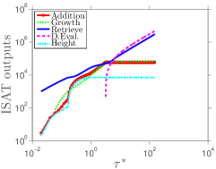
(a) Outputs for case 3.

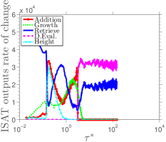
(b) Outputs rates of change for case 3.

Figure 18: Evolution of ISAT algorithm outputs, height of ISAT binary search tree, and the corresponding rates of change.

For case 3, nevertheless, the number of growths is not always smaller than the number of additions. Initially the growths exceed additions by nearly an order of magnitude. After $\tau^{\ast}=0.2$ the additions exceeded the number of growths, only to be overcome again once steady state is reached. This behavior indicates that the ellipsoids of accuracy show a considerable period of adaptation, which allows to access, with precision, a larger portion of the realizable region.

As in the previous cases, after tree saturation, the number of retrieves and direct evaluations exceed the number of additions. The number of direct evaluations overcomes total number of retrieves in approximately 60%, which is not negligible, but less than that observed in case 2. This indicates that the binary search tree covers a significant portion of the realizable region in the composition space. From Figure 18 one can estimate $\tau_{A}/\tau_{DI}\approx 50$ in order that ISAT technique be more efficient than DI.

For case 3, the computational time spent by DI and ISAT are $689\leavevmode\nobreak\ \mathrm{ks}$ and $455\leavevmode\nobreak\ \mathrm{ks}$, respectively. Therefore, a speed-up of 1.5 is observed. In this case, the effect of other values of ISAT error tolerance has not been investigated. This PMSR has 1024 particles and its evolution is computed during $\tau^{\ast}=150$. Thus, the system of governing equations defined by Eq.(8) is solved $7,680,000$ times. In this case ISAT technique allows to save 34%, in terms of computational time. For problems that require solving Eq.(8) several times, one could speculate that ISAT technique would provide an even better performance improvement, since more retrieves are expected when compared with the more costly direct integration.

4.6 Analysis of ISAT memory usage

The studied cases 1 and 2 are both modeled by a reaction mechanism with 4 species and use a binary search tree with 50,000 entries for ISAT simulations. These parameters lead to a memory consumption by ISAT algorithm of approximately $40\leavevmode\nobreak\ \mathrm{Mbytes}$, which is very small when compared with the available memory in the workstation used.

On the other hand, case 3 is modeled by a reaction mechanism with 53 species and use a binary search tree with 60,000 entries. This case uses approximately $3.3\leavevmode\nobreak\ \mathrm{Gbytes}$ of memory. It is noteworthy that this value of memory usage is not negligible, when compared to the total memory available on the workstation. Thus, for practical purposes, this tree is the largest one that may be used to simulate a PMSR with this methane reaction mechanism and 1024 particles. This underscores what is perhaps the greatest shortcoming of ISAT technique, its huge expense of memory.

5 Concluding remarks

This work assessed characteristics of a PMSR reactor through the numerical simulation of reactor configurations with simple ($CO/O_{2}$) and complex ($CH_{4}$/air) reaction mechanisms and also investigated ISAT technique as an option to evaluate a computational model with detailed thermochemistry. For this purpose, the accuracy, performance, and memory usage of the corresponding technique were analyzed through the comparison of ISAT results with a reference result, obtained from direct integration of PMSR model equation. The studied cases analysis showed that ISAT technique has a good accuracy from a global point of view. Also, it was possible to identify the statistical seed effect on the control of absolute global error, which decreases monotonically as ISAT error tolerance was reduced, when the same seed is used for ISAT and DI calculations. On the other hand, when different seeds were used, a limit value for ISAT error tolerance was observed. In terms of performance, ISAT technique allows to reduce the computational time of the simulations in all cases studied. For $CO/O_{2}$ cases, a speed-up of up to 5.0 was achieved, whereas for $CH_{4}$/air, the algorithm allowed to save 34% in terms of computational time. Moreover, ISAT technique presented the desired feature of speed-up factor increase with the complexity of analyzed system. Regarding the memory usage, ISAT technique showed to be very demanding. This work will be extended by coupling ISAT technique to the hybrid LES/PDF model by Andrade et al (2011); Vedovoto et al (2011); Andrade (2009); Vedovoto (2011) for description of turbulent combustion, when a detailed reaction mechanism would allow a better description of combustion. In this context, ISAT could be a viable option that may be able to decrease, to an acceptable level, the simulation time.