Supplemental information for
Quantum control of the tin-vacancy spin qubit in diamond

I Tin-vacancy electronic structure model

I.1 Tin-vacancy Hamiltonian

The ground and excited states of the tin-vacancy (SnV) are composed of two orbital branches, split by the Jahn-Teller, spin-orbit and strain effects, with two spin sublevels each, split by the Zeeman effect [1, 2]. In this subsection, we will present the Hamiltonian for the ground state manifold and use it to gain insight about the character of our spin qubit.

The spin-orbit effect term of the Hamiltonian, expressed with $\{\ket{e_{x}},\ket{e_{y}}\}$ spanning the orbital subspace and $\{\ket{\uparrow},\ket{\downarrow}\}$ the spin subspace, is given by [1]:

$$H_{\textrm{SO}}=\frac{-\lambda_{\textrm{SO}}}{2}\begin{bmatrix}0&i\\ -i&0\end{bmatrix}_{\ket{e_{x}},\ket{e_{y}}}\otimes\begin{bmatrix}1&0\\ 0&-1\end{bmatrix}_{\ket{\uparrow},\ket{\downarrow}}.$$

The eigenstates resulting from the spin-orbit Hamiltonian are:

$$\ket{4}_{\textrm{SO}}=\frac{1}{\sqrt{2}}\left(\ket{e_{x}\uparrow}+i\ket{e_{y}\uparrow}\right)=\ket{e_{+}\uparrow}\textrm{, with energy }\lambda_{\textrm{SO}}/2;$$

$$\ket{3}_{\textrm{SO}}=\frac{1}{\sqrt{2}}\left(\ket{e_{x}\downarrow}-i\ket{e_{y}\downarrow}\right)=\ket{e_{-}\downarrow}\textrm{, with energy }\lambda_{\textrm{SO}}/2;$$

$$\ket{2}_{\textrm{SO}}=\frac{1}{\sqrt{2}}\left(\ket{e_{x}\uparrow}-i\ket{e_{y}\uparrow}\right)=\ket{e_{-}\uparrow}\textrm{, with energy }-\lambda_{\textrm{SO}}/2;$$

$$\ket{1}_{\textrm{SO}}=\frac{1}{\sqrt{2}}\left(\ket{e_{x}\downarrow}+i\ket{e_{y}\downarrow}\right)=\ket{e_{+}\downarrow}\textrm{, with energy }-\lambda_{\textrm{SO}}/2,$$

where $e_{\pm}=\frac{1}{\sqrt{2}}(e_{x}\pm ie_{y})$. This shows that when only spin-orbit is considered, the two lowest energy eigenstates $\ket{1}$ and $\ket{2}$, which form our qubit, are orthogonal in both the orbital and spin subspaces. Since the spin-orbit effect is the dominant effect in the ground state Hamiltonian with $\lambda_{\textrm{SO}}=850$ GHz, we will henceforth express all Hamiltonians in the basis set by the spin-orbit eigenstates $\{\ket{e_{+}},\ket{e_{-}}\}\otimes\{\ket{\uparrow},\ket{\downarrow\}}$:

$$H_{\textrm{SO}}=\frac{\lambda_{\textrm{SO}}}{2}\begin{bmatrix}1&0&0&0\\ 0&-1&0&0\\ 0&0&-1&0\\ 0&0&0&1\\ \end{bmatrix}\\ .$$

The Zeeman effect acts on both the spin and orbital subspaces. The orbital Zeeman effect is heavily quenched by the Jahn-Teller interaction [1] and therefore is commonly neglected [2, 3], as it will be in this work. The spin Zeeman effect is split into the contribution due to magnetic field parallel ($B_{z}$) and perpendicular ($B_{x},B_{y}$) to the SnV spin-orbit axis. The Hamiltonian for the parallel field is given by:

$$H_{Z,\parallel}=\frac{\gamma_{e}}{2}\begin{bmatrix}1&0\\ 0&1\end{bmatrix}\otimes\begin{bmatrix}B_{z}&0\\ 0&-B_{z}\end{bmatrix}$$

with $\gamma_{e}=2\mu_{B}/\hbar$ denoting the electron gyromagnetic ratio. This Hamiltonian is diagonal in the spin-orbit basis, and therefore leaves the eigenstates unchanged. The Hamiltonian for the perpendicular magnetic field is given by:

$$H_{Z,\perp}=\frac{\gamma_{e}}{2}\begin{bmatrix}1&0\\ 0&1\end{bmatrix}\otimes\begin{bmatrix}0&B_{x}-iB_{y}\\ B_{x}+iB_{y}&0\end{bmatrix}.$$

The eigenstates of H = $H_{\textrm{SO}}+H_{\textrm{Z},\parallel}+H_{\textrm{Z},\perp}$ are:

$$\ket{4}_{\textrm{SO}+Z,\parallel+Z,\perp}=\ket{e_{+}}\otimes\left[\ket{\uparrow}+\frac{\gamma_{e}B_{+}}{\gamma_{e}B_{z}+\lambda_{\textrm{SO}}+\sqrt{|\gamma_{e}B_{+}|^{2}+(\lambda_{\textrm{SO}}+\gamma_{e}B_{z})^{2}}}\ket{\downarrow}\right];$$

$$\ket{3}_{\textrm{SO}+Z,\parallel+Z,\perp}=\ket{e_{-}}\otimes\left[\ket{\downarrow}+\frac{\gamma_{e}B_{+}}{-\gamma_{e}B_{z}+\lambda_{\textrm{SO}}+\sqrt{|\gamma_{e}B_{+}|^{2}+(\lambda_{\textrm{SO}}+\gamma_{e}B_{z})^{2}}}\ket{\uparrow}\right];$$

$$\ket{2}_{\textrm{SO}+Z,\parallel+Z,\perp}=\ket{e_{-}}\otimes\left[\ket{\uparrow}-\frac{\gamma_{e}B_{+}}{-\gamma_{e}B_{z}+\lambda_{\textrm{SO}}+\sqrt{|\gamma_{e}B_{+}|^{2}+(\lambda_{\textrm{SO}}+\gamma_{e}B_{z})^{2}}}\ket{\downarrow}\right];$$

$$\ket{1}_{\textrm{SO}+Z,\parallel+Z,\perp}=\ket{e_{+}}\otimes\left[\ket{\downarrow}-\frac{\gamma_{e}B_{+}}{\gamma_{e}B_{z}+\lambda_{\textrm{SO}}+\sqrt{|\gamma_{e}B_{+}|^{2}+(\lambda_{\textrm{SO}}+\gamma_{e}B_{z})^{2}}}\ket{\uparrow}\right],$$

where $B_{+}=B_{x}+iB_{y}$. As shown, a magnetic field perpendicular to the spin-orbit axis mixes the spin states, but does not mix the orbital states. In particular, the two qubit levels still have orthogonal orbital states.

The Jahn-Teller effect acts only on the orbital subspace, and therefore in the spin-orbit basis can be written as:

$$H_{\textrm{JT}}=\begin{bmatrix}a&c\\ c&b\end{bmatrix}\otimes\begin{bmatrix}1&0\\ 0&1\end{bmatrix}.$$

Since this term captures any general effect acting only on the orbital subspace, any strain inherent to the diamond lattice can be expressed into this term. The eigenstates of H = $H_{\textrm{SO}}+H_{Z,\parallel}+H_{\textrm{JT}}$ are:

$$\ket{4}_{\textrm{SO}+Z,\parallel+\textrm{JT}}=\left[\ket{e_{+}}+\frac{2c}{a-b+\lambda_{\textrm{SO}}+\sqrt{4c^{2}+(a-b+\lambda_{\textrm{SO}})^{2}}}\ket{e_{-}}\right]\otimes\ket{\uparrow};$$

$$\ket{3}_{\textrm{SO}+Z,\parallel+\textrm{JT}}=\left[\ket{e_{-}}-\frac{2c}{-a+b+\lambda_{\textrm{SO}}-\sqrt{4c^{2}+(-a+b+\lambda_{\textrm{SO}})^{2}}}\ket{e_{+}}\right]\otimes\ket{\downarrow};$$

$$\ket{2}_{\textrm{SO}+Z,\parallel+\textrm{JT}}=\left[\ket{e_{-}}+\frac{2c}{-a+b-\lambda_{\textrm{SO}}-\sqrt{4c^{2}+(-a+b-\lambda_{\textrm{SO}})^{2}}}\ket{e_{+}}\right]\otimes\ket{\uparrow};$$

$$\ket{1}_{\textrm{SO}+Z,\parallel+\textrm{JT}}=\left[\ket{e_{+}}-\frac{2c}{-a+b+\lambda_{\textrm{SO}}+\sqrt{4c^{2}+(-a+b+\lambda_{\textrm{SO}})^{2}}}\ket{e_{-}}\right]\otimes\ket{\downarrow}.$$

This shows that the $c$ component of the Jahn-Teller (and strain) effect leads to non-zero overlap in the orbital states of the two qubit levels.

I.2 Microwave drive of spin qubit

The Rabi rate from driving our spin qubit with a microwave drive is expected to be proportional to: $\Omega_{\textrm{MW}}\propto\bra{1}H_{\textrm{MW}}\ket{2}$ with

$$H_{\textrm{MW}}=\begin{bmatrix}1&0\\ 0&1\end{bmatrix}\otimes\begin{bmatrix}0&1\\ 1&0\end{bmatrix}$$

since the microwave drive preserves the orbital part of the state. Taking $\ket{1},\ket{2}$ to be the spin qubit as defined by the spin-orbit eigenstates, $\Omega_{\textrm{MW}}=0$ due to the the two qubit levels having orthogonal orbital states. Taking $\ket{1},\ket{2}$ to be the spin qubit as defined by the spin-orbit, parallel Zeeman, and Jahn-Teller (including strain) eigenstates, however gives:

$$\Omega_{\textrm{MW}} \propto\frac{2c}{-a+b-\lambda_{\textrm{SO}}-\sqrt{4c^{2}+(-a+b-\lambda_{\textrm{SO}})^{2}}}\bra{e_{+}}\ket{e_{+}}$$

$$+\frac{2c}{-a+b+\lambda_{\textrm{SO}}+\sqrt{4c^{2}+(-a+b+\lambda_{\textrm{SO}})^{2}}}\bra{e_{-}}\ket{e_{-}}$$

$$=2c\left(\frac{1}{-a+b+\lambda_{\textrm{SO}}+\sqrt{4c^{2}+(-a+b+\lambda_{\textrm{SO}})^{2}}}+\frac{1}{a-b+\lambda_{\textrm{SO}}+\sqrt{4c^{2}+(a-b+\lambda_{\textrm{SO}})^{2}}}\right).$$

To simplify this expression, we note that only the c term type strain contributes to the orbital mixing which enables microwave drive, and thus we consider strain with components such that $a=b$, and assume $\lambda_{\textrm{SO}}\gg c$, which yields:

$$\frac{4c}{\lambda_{\textrm{SO}}+\sqrt{4c^{2}+\lambda_{\textrm{SO}}^{2}}}\approx\frac{2c}{\lambda_{\textrm{SO}}}.$$

This shows that direct microwave drive of the SnV qubit is only allowed due to the Jahn-Teller (and strain) effect. However, as these energy scales (typical strains on this sample are around 10 GHz, while the Jahn-Teller is around 65 GHz [2]) are much smaller than the energy scale of the spin-orbit effect (850 GHz), driving the spin qubit via microwaves is highly inefficient.

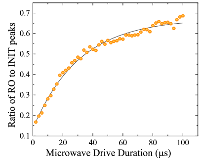
Figure S1: Microwave drive measurement. Ratio of readout pulse peak fluorescence (RO) to initialisation pulse peak fluorescence (INIT) for the emitter measured in [2] as a function of microwave drive duration at 4 K. SnV spin state is prepared in the $\ket{\uparrow}$ state followed by a resonant microwave drive with 10 W of power at the cryostat entry. The solid line is a fit to $1-b(\exp[-t/a])+c$ with $a=31(2)$ $\upmu$s, $b=0.54(1)$, $c=-0.33(1)$.

I.3 Microwave drive results

Figure S1 shows the results of our attempts to drive an SnV with microwave drive. While this SnV is not the same SnV that is studied in the main text, it is from the same part of the device and has similar properties in terms of zero phonon line wavelengths, and ground and excited state gyromagnetic ratios. Analogously to the pulse sequence shown in Fig. 2a, the pulse sequence used here consists of an initialize, drive, and readout pulse. The $\ket{\downarrow}$ population is calculated from the signal intensity observed in the readout pulse normalized by that observed in the initialize pulse. The drive consists of 10 W of microwave power at a frequency resonant with the spin qubit being applied using the same microwave delivery system as in reference [2]. Figure S1 shows the $\ket{\downarrow}$ population as a function of the microwave drive duration $T$. Fitting the recovery in $\ket{\downarrow}$ population to an exponential yields a time constant of 31(2) $\upmu$s, 200 times smaller than what is achieved in the main text with a lambda scheme with 200 nW per Raman drive. Given the coherence time $T_{2}^{*}=1.3(3)\,\upmu$s found in the main text, the microwave drive would need to be over an order of magnitude faster (two orders of magnitude more microwave power) to approach the coherent control regime.

I.4 Realizing a lambda scheme

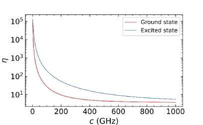
Figure S2: Branching ratio of the lambda scheme when a Jahn-Teller effect with strength $c$ is included in the ground state (red) or in the excited state (blue) for a magnetic field of 0.2 T applied at 54.7º to the symmetry axis of the SnV.

We now apply the Hamiltonian presented above to both the ground and excited states, so as to model the transitions between the two. These transitions are of particular interest as they allow for Raman transitions between the spin ground states.

The Hamiltonian describing the excited state is composed of the same terms as that describing the ground state, presented in SI IIIA [1]. In particular, the Zeeman effect and spin-orbit effect terms have the same matrix representations up to specific energy values. This is because in both the ground and excited states, the Zeeman effect sets a quantization axis along the direction of the applied magnetic field and the spin-orbit effect sets a quantization axis along the SnV symmetry axis [1]. The difference is that while the magnitude of the Zeeman effect is similar in both the ground and excited states, the magnitude of the spin-orbit effect is much higher in the excited state. Specifically, the spin-orbit effect has a strength of $\sim$3000 GHz in the excited state, and largely dominates over the Zeeman splitting ($\sim$4 GHz at $B=0.2$ T) [2]. Given these two terms, the quantization axis for the electronic spin in the excited state is pinned to the symmetry axis of the SnV, and thus $\ket{\textrm{A}}=\ket{e_{+}\downarrow}$. In the ground state, the spin-orbit contribution is weaker, and perturbs the eigenstates, which to first order become $\ket{1}\approx\ket{e_{+}}\otimes\big{[}\ket{\downarrow}-\frac{\gamma_{e}B_{+}}{2\lambda_{\textrm{SO}}}\ket{\uparrow}\big{]}$ and $\ket{2}\approx\ket{e_{-}}\otimes\big{[}\ket{\uparrow}-\frac{\gamma_{e}B_{+}}{2\lambda_{\textrm{SO}}}\ket{\downarrow}\big{]}$

The dipole operator enabling optical transitions driven by unpolarized light between the excited state $\ket{\textrm{A}}$ and the ground state qubit levels $\ket{1}$ and $\ket{2}$ acts as the identity in the spin basis and has components in the orbital subspace given in the ${\ket{e_{+}},\ket{e_{-}}}$ basis by [1]

$$\hat{p}_{x}=\begin{bmatrix}0&1\\ 1&0\end{bmatrix},\hat{p}_{y}=\begin{bmatrix}0&-i\\ i&0\end{bmatrix},\hat{p}_{z}=\begin{bmatrix}2&0\\ 0&2\end{bmatrix}.$$

Thus, from Fermi’s golden rule, the expected strength of the A1 “spin conserving” optical transition is proportional to:

$$|\bra{A}\hat{p}\ket{1}|^{2}{} =|\bra{A}\hat{p}_{x}\ket{1}|^{2}+|\bra{A}\hat{p}_{y}\ket{1}|^{2}+|\bra{A}\hat{p}_{z}\ket{1}|^{2}$$

$$=|\bra{A}\hat{p}_{z}\ket{1}|^{2}$$

$$=4,$$

and that of the A2 “spin flipping” optical transition is proportional to:

$$|\bra{A}\hat{p}\ket{2}|^{2}{} =|\bra{A}\hat{p}_{x}\ket{2}|^{2}+|\bra{A}\hat{p}_{y}\ket{2}|^{2}+|\bra{A}\hat{p}_{z}\ket{2}|^{2}$$

$$=2~{}\left|\bra{\downarrow}~{}\left(\ket{\uparrow}-\frac{\gamma_{e}B_{+}}{2\lambda_{\textrm{SO}}}\ket{\downarrow}\right)\right|^{2}$$

$$=\frac{\gamma_{e}^{2}B_{+}^{2}}{2\lambda_{\textrm{SO}}^{2}}.$$

This demonstrates that under an off-axis magnetic field the “spin-flipping” A1 transition becomes allowed. Nevertheless, given the large $\lambda_{\text{SO}}$ of SnV, this transition is still largely suppressed. Figure S2 presents a numerical simulation of the branching ratio when a Jahn-Teller term with $a=b=0$ and varying $c$ is also included [2]. It shows that the Jahn-Teller effect in the ground or excited state can explain the more balanced fraction in the Rabi rates of $\sim 100$ measured in this work. As this term can also be induced by strain, the branching ratio can vary between different emitters.

Driving these two transitions results in a lambda scheme between the two qubit states and a shared excited state which can be used to drive the spin qubit all-optically. Whereas control techniques relying on directly driving the spin qubit magnetically face the challenge of the spin qubit having near orthogonal orbital degrees of freedom, the all-optical control technique circumvents this issue by relying on the optical electric dipole moments featuring more relaxed orbital selection rules. The efficacy of this scheme depends on (1) the ratio of the decay rates for the A1 and A2 transitions, a parameter we define as $\eta$, and (2) how well light is able to couple to the SnV and drive these transitions, quantified by the saturation power of the A1 transition $p_{\textrm{sat}}$.

II Characterization of tin-vacancy lambda scheme parameters

In this section, we analyze the time-resolved counts obtained during an initialize pulse and use this to obtain values for the initialization fidelity as well as $\eta$ and $p_{\textrm{sat}}$. Figure S3 shows an example of the fluorescence measured during an initialize pulse (preceded by a reset pulse to ensure $\sim$100% population in the $\ket{\downarrow}$ state), where a resonant laser drives A1. The fluorescence signal is proportional to the population being driven by the A1 drive. The signal decreases exponentially over time as population decays from the $\ket{1\downarrow}$ state to the $\ket{2\uparrow}$ state via the spin-flipping transition A2. Taking the ratio of the fluorescence in the first time bin to that in the steady state time bins, minus background counts, we find $\epsilon$ = 0.9% of the population remaining in the $\ket{\downarrow}$ state. We thus extract an initialization fidelity $F_{\textrm{init}}=1-\frac{\epsilon}{2}\,=\,99.6$%. This measured value of initialization fidelity could be limited by resonant laser leakage past our 633 nm longpass filter and by off-resonant excitation of the B2 transition, both of which prevent the steady state counts from dropping to zero. The latter issue could be suppressed by working at higher magnetic fields or lower powers such that off resonant excitation of the B2 transition is lowered.

The initialization measurement explained above is repeated at various laser powers $p$. For each $p$, the fluorescence counts are fit to an exponential decay to extract the initialization rate, defined as the inverse of the exponential time constant, presented in $\mathrm{{Fig.}\,\ref{fig:inittimeconstants}}$. Fitting the initialization rates to $\frac{\Gamma}{2}\frac{p/p_{\textrm{sat}}}{1+p/p_{\textrm{sat}}}\frac{1}{\eta}$ [4], we find $p_{\textrm{sat}}\,=4.6(7)$ nW and $\eta\,=\,80(5)$.

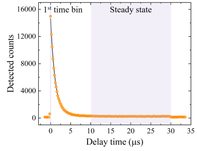
Figure S3: Fluorescence during resonant drive measurement. APD counts during a 30 $\upmu$s long A1 pulse plotted in orange circles as a function of time. The solid curve is a fit to $a\textrm{exp}[-t/\tau_{\textrm{init}}]+c$ resulting in $\tau_{\textrm{init}}=1.2(1)$ $\upmu$s. The first time bin includes 14968 counts, the average of the steady state time bins is 281 counts, and the background is 141 counts.

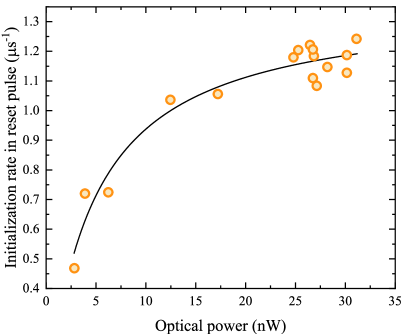
Figure S4: Initialization rate for different laser powers. The initialization rates are plotted in orange circles as a function of initialization drive laser power. The solid curve is a fit to $\frac{\Gamma}{2}\frac{p/p_{\textrm{sat}}}{1+p/p_{\textrm{sat}}}\frac{1}{\eta}$ resulting in $p_{\textrm{sat}}\,=\,4.6(7)$ nW and $\eta\,=\,80(5)$.

III Modelling all-optical coherent control

In this section, we first present an analytical model describing all-optical Rabi and apply it to the Rabi measurements presented in Fig. 2a. We then develop a master equation model, and compare the results from the analytical model to those extracted by fitting the master equation model to the measured data. The consistency between the models confirms our understanding of the physics captured in the Rabi measurements. Finally, we comment on a key metric of our all-optical gates: their gate fidelity.

III.1 Analytical model

We consider the lambda system presented in Fig. 1a, consisting of two spin ground states $\ket{\downarrow}$ and $\ket{\uparrow}$ and an excited state $\ket{\textrm{E}}$ with a natural linewidth $\Gamma$ driven by two laser fields at frequencies $\omega_{1,2}$. The optical Rabi rate achieved by $\omega_{1}$, driving the spin-cycling optical transition A1, is given by $\Omega_{1}=\frac{1}{\sqrt{2}}\sqrt{s}\Gamma$, where $s=\frac{p}{p_{\textrm{sat}}}$ is the saturation parameter [4]. The Rabi rate achieved by $\omega_{2}$, driving the weakly allowed spin-flipping optical transition A2, is given by $\Omega_{2}=\frac{1}{\sqrt{\eta}}\Omega_{1}=\frac{1}{\sqrt{2\eta}}\sqrt{s}\Gamma$. By driving $\omega_{1,2}$ simultaneously at a single photon detuning $\Delta$, the two ground states are driven with a Rabi rate of $\Omega=\frac{\Omega_{1}\Omega_{2}}{2\Delta}=\frac{s\Gamma^{2}}{\sqrt{\eta}4\Delta}$.

Driving $\omega_{1,2}$ will also result in scattering off the excited state at a rate given by $\Gamma_{\textrm{os}}=\frac{s\Gamma^{3}}{8\Delta^{2}}$ in the limit of large $\Delta$ ($\Delta>\sqrt{s}\Gamma$). Each scattering event results in a phase given by $\omega_{e}/\Gamma$ being accrued, and therefore leads to decoherence. Due to this, the spin coherence time cannot exceed $T_{2,\textrm{os}}=\frac{1}{\Gamma_{\textrm{os}}}$. This phenomenon also sets an upper bound on the spin lifetime $T_{1,\textrm{os}}=\frac{\eta}{\Gamma_{\textrm{os}}}$, as one in every $\eta$ scattering events results in a spin flip.

We now apply the equations derived in our analytical model, $\Omega=\frac{s\Gamma^{2}}{\sqrt{\eta}4\Delta}$ and $\Gamma_{\textrm{os}}=\frac{s\Gamma^{3}}{8\Delta^{2}}$, to the case of the Rabi measurements in Fig. 2a. In these equations, we set $\eta=80$ and $p_{\textrm{sat}}=4.6$ nW as found in SI section II. The single photon detuning is set to $\Delta/2\pi=1200$ MHz, and $p$ is set to 650 nW, as in the measurements presented in Fig. 2a. Using these values, the analytical model predicts $\Omega/2\pi=3.9(9)$ MHz and $\Gamma_{\textrm{os}}=3.3(6)$ $\upmu\textrm{s}^{-1}$.

III.2 Master equation model

We will now describe a 2-level model under a master equation formalism that can be fit to the Rabi measurements presented in Fig 2a. In this model, the von Neumann equation acquires a non-unitary term, known as the Lindbladian super-operator, which models Markovian decoherence dynamics [5]:

$$\frac{\partial\rho}{\partial t}=\frac{-i}{\hbar}[H,\rho]+\sum_{i}c_{i}\rho c_{i}^{\dagger}-\frac{1}{2}(c_{i}^{\dagger}c_{i}\rho+\rho c_{i}^{\dagger}c_{i}),$$

where $\{c_{i}\}$ are the set of collapse operators and $\rho$ is the density operator. In this model, unitary evolution is driven by the Hamiltonian:

$$H=\frac{\Omega}{2}\sigma_{x}+\frac{\delta}{2}\sigma_{z},$$

where $\sigma_{i}$ is the $i$’th Pauli matrix, $\Omega$ the Rabi rate and $\delta$ the two-photon detuning. The collapse operators are given by:

$$c_{1}=\sqrt{\frac{\gamma_{1}}{2}}\sigma_{x};$$

$$c_{2}=\sqrt{\frac{\gamma_{2}}{2}}\sigma_{z},$$

where $c_{1}$ describes $T_{1}$ depolarisation, with depolarisation rate $\gamma_{1}$ and $c_{2}$ describes $T_{2}$ pure dephasing, with pure dephasing rate $\gamma_{2}$. To account for non-Markovian inhomogenous dephasing mechanisms, leading to $T_{2}^{*}$ limited coherence times without dynamical decoupling, a phenomenological model was adopted. In this model two-photon detunings are sampled from a normal distribution with standard deviation $\frac{1}{T_{2}^{*}}$ [6, 7], and averaged together; just as how slow inhomogenous dephasing manifests itself experimentally. Finally, to account for $T_{1}$ depolarisation amongst the 4-level electro-nuclear manifold on the time-scales probed in Fig. 2 of the main text, a Rabi-visibility depolarisation term of the form $\frac{1}{4}(1-e^{-T\frac{\gamma_{1}}{2\pi}})$ was included in the model. In this formalism, $T$ is the Raman drive time in Fig. 2, and this response is added to the 2-level model to yield the final model with free parameters $\Omega$, $\gamma_{1}$ and $\gamma_{2}$.

Fitting this master equation model to the Rabi measurements (as presented in Fig. 2a), we obtain $\Omega/2\pi=3.6(1)$ MHz and a pure dephasing rate, $\gamma_{T_{2}}$, of 7(4)$\,\upmu\textrm{s}^{-1}$. As the analytically derived $\Gamma_{\textrm{os}}$ is within the confidence interval of the extracted pure dephasing rate, we conclude that the pure dephasing rate is dominated by the optical scattering process described above. The consistency between the analytically derived expressions and the measured data confirms that the analysis of section A captures the salient physics involved in our all-optical control scheme.

III.3 Gate fidelities

We will now comment on a key metric of the gates realized via our all-optical control scheme, the $\pi/2$ gate fidelity. For a $\pi/2$ gate limited by a $T_{1}$ process such as optical scattering, the gate fidelity can be defined as $F_{\pi/2}=0.5(1+\textrm{exp}(-1/Q_{\pi/2})]$, where $Q_{\pi/2}=(16/9)\Omega/\Gamma_{\textrm{os}}$. Using the $\Omega/2\pi=3.6(1)$ MHz and $\Gamma_{\textrm{os}}=7(4)$ $\upmu$s^-1 values reported in Fig. 2a, we calculate $F_{\pi/2}=0.92(4)$. As this value is limited by optical scattering, it could be improved by increasing $\Delta$.

Figure SI 5 shows the expected fidelity of gates performed at various $s$ and $\Delta$. To include infidelities introduced by inhomogeneous dephasing, we extend the definition presented above to $Q_{\pi/2}=(16/9)\Omega/\Gamma_{\textrm{tot}}$, where $\Gamma_{\textrm{tot}}=\textrm{max}[\Gamma_{\textrm{os}},\,1/T_{2}^{*}]$, where $T_{2}^{*}\,=\,1.3\,\upmu$s as found in Fig. 3a. For fixed $s$, in the regime $\Delta<\sqrt{s\Gamma^{3}T_{2}^{*}/8}$ the gate fidelity is limited by optical scattering, whereas for $\Delta>\sqrt{s\Gamma^{3}T_{2}^{*}/8}$ the gate fidelity is limited by the quasi-static noise bath responsible for $T_{2}^{*}$.

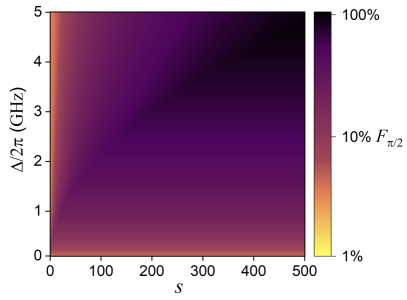
Figure S5: Rabi gate fidelity simulation. Plot of the $\pi/2$ gate fidelity $F_{\pi/2}$ as a function of $\Delta$ and $s$.

IV Sample fabrication

The sample is the same as that used in Ref. [2]. The diamond is an Element6 CVD-grown type IIa diamond with $<$ 5 ppb [N],[B]. Sn+ ions were implanted with a fluence of $10^{9}$ ions/cm² and at an energy of 350 keV for a predicted dopant depth of 80(10) nm below the diamond surface as modeled by Stopping Range of Ions in Matter simulations. The sample was then annealed at $1200^{\circ}$ C for two hours under high vacuum ($<10^{-7}$ mbar) and subsequently cleaned in a 1:1:1 mixture of boiling sulfuric, nitric and perchloric acid to remove residual graphite. Finally nanopillars (radii 75 to 165 nm), shown in $\mathrm{{Fig.}\,\ref{fig:pillars}}$, were fabricated to improve fluorescence collection efficiency and to isolate individual SnV centers.

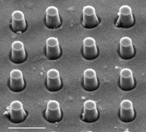
Figure S6: Scanning electron micrograph of the fabricated nanopillars. Scale bar is 1 $\upmu$m.

V Equipment set-up

V.1 Experimental details on primary optical system

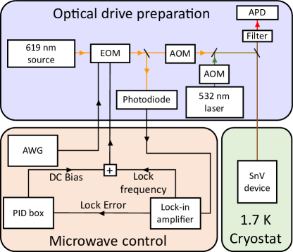
Figure S7: Schematic of experimental setup. Optical drive preparation in the blue panel: 619 nm light passes through an EOM to generate sidebands. Pulse timings for the 619 nm and 532 nm lasers are implemented by acoustic-optic modulators (AOMs). Emission from the sample is separated from the excitation path using a 70:30 non-polarizing beamsplitter. The light is filtered by a 633 nm long-pass filter and sent to an avalanche photodiode (APD). Microwave control in the orange panel includes an arbitrary waveform generator (AWG) as well as a lock-in amplifier and PID box to stabilize the EOM setpoint. The optical cryostat in the green box cools sample to 1.7 K and enables the application of magnetic fields.

The optical fields used to drive the lambda system are two sidebands generated on a single laser source by an amplitude electro-optic modulator (Jenoptik AM635), and the amplitude, phase, and frequency of the sidebands are controlled by a 25 Gs$/$sec arbitrary waveform generator (Tektronix AWG70002A). Reset and initialize/readout pulses are generated by changing the AWG microwave frequency such that the EOM sidebands are resonant with the A2 and A1 transitions respectively. The EOM is locked to its interferometric minimum by modulating it with a reference signal from a lock-in amplifier (SRS SR830 DSP Lock-in Amplifier) at f = 9.964 kHz with a feedback loop on the signal generated by a photodetector (Thorlabs PDA100A2). The error signal is sent to a PID (SRS SIM960 Analog PID Controller), whose output is applied to the EOM by a bias-tee.

The data shown in the measurements presented in this work were taken in a closed-cycle cryostat (attoDRY 2100) with a base temperature of 1.7 K at the sample and in which the temperature can be tuned with a resistive heater located under the sample mount. Superconducting coils around the sample space allow the application of a vertical magnetic field from 0 to 9 T and a horizontal magnetic field from 0 to 1 T. Unless explicitly stated otherwise, all measurements were conducted at T=1.7 K and B=0.2 T with the magnetic field orientation 54.7 ^∘ rotated from the SnV symmetry axis. The optical part of the set-up consists of a confocal microscope mounted on top of the cryostat and a microscope objective with numerical aperture 0.82 inside the cryostat. The sample is moved with respect to the objective utilizing piezoelectric stages (ANPx101/LT and ANPz101/LT) on top of which the sample is mounted. Resonant excitation around 619 nm is performed by a second harmonic generation stage (ADVR RSH-T0619-P13FSAL0) consisting of a frequency doubler crystal pumped by a 1238 nm diode laser (Sacher Lasertechnik Lynx TEC 150). The frequency is continuously stabilized through feedback from a wavemeter (High Finesse WSU). The charge environment of the SnV- is reset with microsecond pulses at 532 nm (M-squared Equinox). Optical pulses are generated with an acousto-optic modulator (Gooch and Housego 3080-15) controlled by a delay generator (Stanford Research Instruments DG645). For resonant excitation measurements, a long-pass filter at 630 nm (Semrock BLP01-633R-25) is used to separate the fluorescence from the phonon-sideband from the laser light. The fluorescence is then sent to a single photon counting module (SPCM-AQRH-TR), which generates TTL pulses sent to a time-to-digital converter (Swabian Timetagger20) triggered by an arbitrary waveform generator (Tektronix AWG70002A). Photon counts during “initialize” and “readout” pulses are histogrammed in the time-tagger to measure the $\ket{\downarrow}$ population as described in the main text.

V.2 Experimental details on second optical system

The data in $\mathrm{{Fig.}\,\ref{fig:CPT}}$ is measured in a BlueFors He dilution refrigerator at 3.2 K. The sample consists of an SnV implanted in a diamond microchiplet with several waveguides. A lensed fiber (OZ Optics TSMJ-3U-1550-9/125-0.25-7-2.5-14-2) is used to collect PL, which is filtered to measure the phonon sideband. The sample is placed in a static magnetic field $\sim$ 0.1 T produced by a permanent magnet. Coherent population trapping (CPT) is measured using the same pulse sequence described in the main text but with rest on A2 instead of A1.

V.3 Measurement conditions for main-text data

The coherent control used throughout the main text requires that we measure the spin Rabi rate to determine the drive duration required to produce $\pi/2$ and $\pi$ rotations. In Table S1, we present a summary of the single-photon detuning $\Delta$ and power-per-sideband $p$ used in each figure.

Main text figure	1b	1c	2a	2b	3	4 (Hahn echo)	4 (CPMG-2)
$\Delta/2\pi$ (MHz)	0	600	1200	300	300	600	800
$p$ (nW)	40	40	650	260	260	200	200

Table S1: Table of measurement parameters, single-photon detuning $\Delta$ and power $p$ per sideband with uncertainty taken to be 10%, for data presented in the main text.

VI Coherent population trapping model and simulations

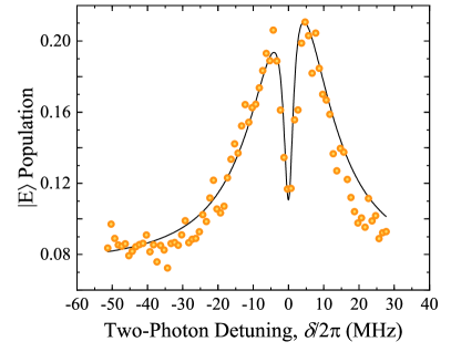
Figure S8: Coherent population trapping measured on an SnV without a hyperfine splitting and $\sim 600$ nW per sideband. The solid curve is a fit to the aforementioned CPT model with the following free-parameters: $\gamma_{\downarrow,\uparrow}=0.2(1)$ MHz, $\gamma_{\downarrow\downarrow,\uparrow\uparrow}=2.72(7)$ MHz, $\Omega=8.0(6)$ MHz and $\Delta=0.9(2)$ MHz.

To model the CPT outlined in Fig. 1b of the main text, we use a three level quantum system, where $\ket{\downarrow}$ and $\ket{\uparrow}$ are the ground states and $\ket{\textrm{E}}$ is the excited state. In the rotating-frame of the $\ket{\downarrow}\leftrightarrow\ket{\textrm{E}}$ the Hamiltonian is given by [8]:

$$\hbar\begin{pmatrix}-\Delta&0&\frac{\Omega_{1}}{2}\\ 0&-\delta&\frac{\Omega_{2}}{2}\\ \frac{\Omega_{1}}{2}&\frac{\Omega_{2}}{2}&0\end{pmatrix},$$

where $\Delta$ is the single-photon detuning, $\delta$ is the two-photon detuning and $\Omega_{1}$ ($\Omega_{2}$) is the Rabi rate between $\ket{\downarrow}$ ($\ket{\uparrow}$) and the excited state $\ket{\textrm{E}}$. Given the cyclicity of SnV, the two Rabi rates are related by $\frac{\Omega_{1}}{\sqrt{f}}=\frac{\Omega_{2}}{\sqrt{1-f}}$, where $f$ is the acyclicity of the lambda scheme and is related to the branching ratio, $\eta$, by $\frac{f}{(1-f)}=\frac{1}{\eta}$.

This Hamiltonian drives unitary evolution of the system’s state-vector between its eigenstates, as determined by the von Neumann equation. At two-photon resonance, these eigenstates coalesce into:

$$\ket{B_{+}}=\sin\theta\sin\phi\ket{\downarrow}+\cos\phi\ket{\textrm{E}}+\cos\theta\sin\phi\ket{\uparrow}$$

$$\ket{B_{-}}=\sin\theta\cos\phi\ket{\downarrow}-\sin\phi\ket{\textrm{E}}+\cos\theta\cos\phi\ket{\uparrow}$$

$$\ket{D}=\cos\theta\ket{\downarrow}-\sin\theta\ket{\uparrow},$$

where $\tan\theta=\frac{\Omega_{1}}{\Omega_{2}}$ and $\tan 2\phi=\frac{\sqrt{\Omega_{1}^{2}+\Omega_{2}^{2}}}{\delta}$. Crucially, the new ground state $\ket{D}$ is orthogonal to the excited state $\ket{\textrm{E}}$ and is therefore dark. Accordingly, scattering from the lambda scheme pumps population into the dark state, as seen by an absence of counts at two-photon resonance.

However, non-unitary dissipative dynamics interfere with the coherence of the lambda scheme and enable scattering from the excited state, even at two-photon resonance. As the generator of Markovian dissipative dynamics, the Lindblad master-equation is suited to model such decoherence dynamics [5]:

$$\frac{\partial\rho}{\partial t}=\frac{-i}{\hbar}[H,\rho]+\sum_{i}c_{i}\rho c_{i}^{\dagger}-\frac{1}{2}(c_{i}^{\dagger}c_{i}\rho+\rho c_{i}^{\dagger}c_{i}),$$

where $\{c_{i}\}$ are the set of collapse operators and $\rho$ is the density operator. Accordingly, the pure-dephasing collapse-operator is given by:

$$\sqrt{\frac{\gamma_{\downarrow\downarrow,\uparrow\uparrow}}{2}}(\ket{\downarrow}\bra{\downarrow}+\ket{\uparrow}\bra{\uparrow}),$$

where $\gamma_{\downarrow\downarrow,\uparrow\uparrow}$ is the inhomogeneous dephasing rate, modelled here as a pure-dephasing rate. Scattering rates from the excited state into $\ket{\downarrow}$ and $\ket{\uparrow}$ are given by

$$\sqrt{\frac{\gamma_{\downarrow,\textrm{E}}}{2}}\ket{\downarrow}\bra{\textrm{E}},$$

$$\sqrt{\frac{\gamma_{\uparrow,\textrm{E}}}{2}}\ket{\uparrow}\bra{\textrm{E}},$$

respectively. The cyclicity of the SnV enforces the constraint $\frac{\gamma_{\downarrow,\textrm{E}}}{f}=\frac{\gamma_{\uparrow,\textrm{E}}}{1-f}$, which is equal to the excited-state scattering rate. Finally, the external bath coupled to the SnV centre induces relaxation parameterised by:

$$\sqrt{\frac{\gamma_{\downarrow,\uparrow}}{2}}(\ket{\downarrow}\bra{\uparrow}+\ket{\uparrow}\bra{\downarrow}),$$

where $\gamma_{\downarrow,\uparrow}$ is the $T_{1}$ dephasing rate. Fitting this model recreates the data presented in Fig. 1b and implies that the hyperfine-interaction induces a 43.6(8) MHz shift in the two-photon detuning between the electro-nuclear spin manifold. The remaining fit parameters are shown to be:

$$\frac{\Omega_{1}}{\sqrt{f}}=\frac{\Omega_{2}}{\sqrt{1-f}}=24.7(1.0)\text{\,MHz}$$

$$\Delta=-2.72(58)\text{\,MHz}$$

and an excited state decay rate $\Gamma/2\pi=32(8)$ MHz.

In $\mathrm{{Fig.}\,\ref{fig:CPT}}$, we furthermore provide a measure of CPT on an SnV in a device measured at 3.2 K in a BlueFors He4-He3 dilution refrigerator. The data in $\mathrm{{Fig.}\,\ref{fig:CPT}}$ was measured using the same sequence in Fig. 1b of the main text, but with reset on A2 in stead of on A1.

VII Intensity-correlation measurement under resonant excitation

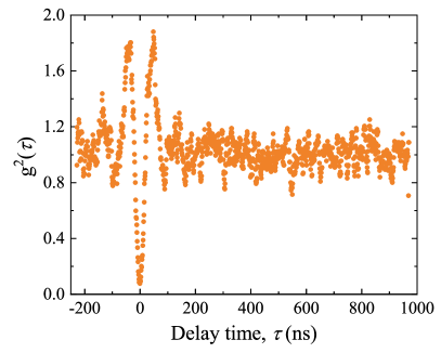
Figure S9: Intensity auto-correlation g²($\tau$) measurement. $g^{2}(\tau)$ measured as a function of $\tau$, plotted as orange circles and connected by a solid line. This measurement was taken at 0 magnetic field such that all four optical transitions (A1, A2, B1, B2) are simultaneously driven with a resonant laser. At $\tau=0$, the measured autocorrelation value reaches a minimum value of $g^{2}(0)$ = $0.08(1)$.

Figure S9 presents a g²($\tau$) auto-correlation measurement on the SnV featured in the main text. The measured $g^{2}(0)=0.08(1)$ unambiguously confirming that we measure a single SnV. We collect emission into the phonon sideband (as in main text) and excite the emitter with continuous-wave resonant excitation at zero magnetic field.

VIII Ramsey signal analysis

VIII.1 Serrodyne frequency $\omega_{\textrm{S}}$

The serrodyne frequency causes the phase of the second $\pi$/2 pulse, $\phi$, to be modulated periodically as a function of the delay duration $\tau$, $\phi=\omega_{\textrm{S}}\tau$. In the absence of two-photon detuning and AC Stark effect ($\delta=\Delta_{\textrm{AC}}=0$), this would rotate the axis of the second $\pi$/2 pulse at a rate $\omega_{\textrm{S}}$, and therefore introduce oscillations in the $\ket{\downarrow}$ population with frequency $\omega_{\textrm{Ramsey}}=\omega_{\textrm{S}}$.

VIII.2 Two-photon detuning $\delta$

When the two photon detuning is nonzero, the rotating frame of the drive, set by $\omega_{R}$, is no longer the same as the rotating frame set by $\omega_{e}$. Therefore, in the rotating frame set by $\omega_{e}$, the drive axis precesses at a rate $\delta=\omega_{R}-\omega_{e}$. Including the effects of both the serrodyne frequency and detuning, the angle between the axis of the state and the axis of rotation is $\phi+\delta(\tau+2T_{\pi/2})=\tau(\omega_{\textrm{S}}+\delta)+2\delta T_{\pi/2}$, where $2T_{\pi/2}$ is the cumulative duration of the two $\pi/2$ pulses. This results in $\omega_{\textrm{Ramsey}}=\omega_{\textrm{S}}+\delta$. The $2\delta T_{\pi/2}$ term captures the precession due to the two-photon detuning during the $\pi$/2 pulses, and explains the phase shift between different horizontal line cuts observed in Fig. 3b.

VIII.3 Differential AC Stark effect $\Delta_{\textrm{AC}}$

The differential AC Stark effect arises due to the difference in AC Stark shifts experienced by the two spin-cycling transitions (A1 and B2). While the drive pulse is on, the spin qubit splitting is increased by $\Delta_{\textrm{AC}}$ and is what we measure as $\omega_{e}$. During the delay time, when the spin qubit is no longer subject to the drive pulse causing the AC Stark shifts, the spin qubit splitting is $\omega_{e}-\Delta_{\textrm{AC}}$. This means that in the $\omega_{e}$ rotating frame, the spin qubit will precess at a rate $-\Delta_{\textrm{AC}}$ during the delay time. The accumulated angle between the axis of the state and the axis of rotation is then $\phi+\delta(\tau+2T_{\pi/2})+\Delta_{\textrm{AC}}\tau=\tau(\omega_{\textrm{S}}+\delta+\Delta_{\textrm{AC}})+2\delta T_{\pi/2}$. This results in $\omega_{\textrm{Ramsey}}=\omega_{\textrm{S}}+\delta+\Delta_{\textrm{AC}}$.

The magnitude of $\Delta_{\textrm{AC}}$ can be calculated by applying the all-optical drive model presented in SI V. Using $\Omega/2\pi=1.4$ MHz, $\eta=80(5)$, and single-photon detuning for the spin-conserving transition $\Delta_{1}/2\pi=300(5)$ MHz, we find an optical Rabi rate $\Omega_{1}/2\pi=87(4)$ MHz. The splitting in the dressed state is $\sqrt{\Omega_{1}^{2}+\Delta_{1}^{2}}$, and the $\ket{\downarrow}$ ground state shifts relative to the undriven case by the AC Stark shift $\Delta_{\textrm{AC,1}}=\frac{\sqrt{\Omega_{1}^{2}+\Delta_{1}^{2}}-\Delta_{1}}{2}\approx\Omega_{1}^{2}/(4\Delta_{1})$. Then $\Delta_{\textrm{AC,1}}/2\pi=6.3(6)$ MHz. The same optical drive is experienced by the $\ket{\uparrow}$ spin-cycling transition but at a detuning $\Delta_{2}=\Delta_{1}+(\omega_{\uparrow\uparrow}-\omega_{\downarrow\downarrow})$, where $(\omega_{\uparrow\uparrow}-\omega_{\downarrow\downarrow})$ is the difference in energy between the spin-conserving transitions, 610(5) MHz. In this case, the shift in the $\ket{\uparrow}$ ground state is $\Delta_{\textrm{AC,2}}/2\pi\approx\Omega_{1}^{2}/(4\Delta_{2})=2.1(2)$ MHz, where the spin-conserving optical Rabi rates are assumed to be equal for $\ket{\downarrow}$ and $\ket{\uparrow}$ and $\Delta_{2}=910(10)$ MHz. The differential AC Stark shift is then $\Delta_{\textrm{AC}}=\Delta_{\textrm{AC,1}}-\Delta_{\textrm{AC,2}}=4.2(8)$ MHz, which we find is in reasonable agreement with the measured value for $\Delta_{\textrm{AC}}=3.3(5)$ MHz. We have neglected contributions from AC Stark effects due to spin-flipping transitions for which the optical Rabi rate is $\sqrt{\eta}$ times weaker, resulting in a $\sim 1$% correction to our estimate for $\Delta_{\textrm{AC}}$. We also neglect the AC Stark shifts due to $\omega_{2}$ detuned from the spin-conserving peaks by $\sim 4$ GHz, which would be a $\sim 10$% correction to our estimated value.

VIII.4 Ramsey simulation

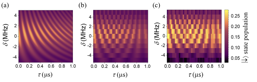
Figure S10: Ramsey fit and comparison to data. (a) Fine-step (1 ns and 10 kHz) simulation for $\ket{\downarrow}$ state population as a function of $\delta$ and $\tau$ obtained from the model in $\mathrm{{Eq.\,SI}\,\ref{eqt:Ramsey}}$. (b) Coarse step simulation. Same as (a) but with the simulation step size for $\delta$ = 1 MHz and the simulation step size for $\tau$ = 25 ns, the same step sizes used in the measurement of Fig. 3b. (c) Reproduction of Fig. 3b data for comparison.

Figure S10a plots the predicted $\ket{\downarrow}$ population obtained from the model

$$\frac{c_{0}}{1+(\delta/c_{1})^{2}}\textrm{exp}[-(\tau/T_{2}^{*})^{2}]\Big{(}\textrm{cos}\big{(}\omega_{\textrm{Ramsey}}\tau+2\delta T_{\pi/2}\big{)}+1\Big{)}+\frac{c_{2}}{1+(\delta/c_{1})^{2}}$$ (1)

where $\omega_{\textrm{Ramsey}}=\omega_{\textrm{S}}+\delta+\Delta_{\textrm{AC}}$, $T_{\pi/2}$ is fixed to the experimentally measured $\pi$/2 gate time, $T_{2}^{*}$ is fixed to the measured inhomogeneous dephasing time found in Fig. 3a, and $\Delta_{\textrm{AC}},\,c_{0}$,  $c_{1}$,  $c_{2}$ are fitting parameters. Figure S10b evaluates the same expression at the time steps taken experimentally in Fig. 3b (reproduced as $\mathrm{{Fig.}\,\ref{fig:ramsey1MHZ}}$c), showing that certain visual artifacts in Fig. 3b (i.e. the lack of $\ket{\downarrow}$ population at $\tau$=900 ns for all measured $\delta$) are simply a result of the aliasing effect from a finite sampling of the time and detuning axes.

IX Spin lifetime $T_{1}$ measurement

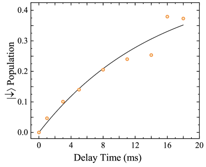
Figure S11: $T_{1}$ measurement under laser leakage. The pulse sequence consists of reset, initialize, delay, and readout pulses, as described in the main text. Orange circles represent $\ket{\downarrow}$ state population recovery as a function of delay time $\tau$. The recovery is fit to $0.5*(1-e^{-\tau/T_{1}})$ (solid line), from which we extract $T_{1}$ = 15(1) ms.

In this section, we present spin lifetime $T_{1}$ measurements taken with 1.0(1) nW of laser leakage at 1.2 GHz detuned from the A1 optical transition. These measurements consist of a reset, initialize, delay, and readout pulses, as described in the main text. Figure S10 presents the recovery of $\ket{\downarrow}$ population as a function of the delay time. We extract $T_{1}$=15(1) ms from this data. As the expected limit on $T_{1}$ from interorbital phonons at 1.7 K is $T_{1,\textrm{phonons}}\,\gg 1$ s [2], we conclude the measured $T_{1}$ is not limited by phonons. In contrast, using the equations derived in SI section III we calculate that the optical scattering due to the laser leakage would limit $T_{1}\leq$  16(2) ms and $T_{2}\,\leq\,$0.20(3) ms. As these values are with error of the $T_{1}$ measurement presented in this section and the $T_{2}$ measurement presented in Fig. 4, we conclude that these measurements were limited by optical scattering.

References

- Hepp et al. [2014] C. Hepp, T. Müller, V. Waselowski, J. N. Becker, B. Pingault, H. Sternschulte, D. Steinmüller-Nethl, A. Gali, J. R. Maze, and M. Atatüre et. al., Electronic Structure of the Silicon Vacancy Color Center in Diamond, Phys. Rev. Lett. 112, 036405 (2014).
- Trusheim et al. [2020] M. E. Trusheim, B. Pingault, N. H. Wan, M. Gündoǧan, L. De Santis, R. Debroux, D. Gangloff, C. Purser, K. C. Chen, and M. Walsh et. al., Transform-Limited Photons from a Coherent Tin-Vacancy Spin in Diamond, Phys. Rev. Lett. 124, 023602 (2020).
- Maity et al. [2020] S. Maity, L. Shao, S. Bogdanović, S. Meesala, Y. I. Sohn, N. Sinclair, B. Pingault, M. Chalupnik, C. Chia, and L. Zheng et. al., Coherent acoustic control of a single silicon vacancy spin in diamond, Nat. Commun. 11, 193 (2020).
- Foot [2005] C. J. Foot, Atomic Physics (Oxford University Press, Oxford, 2005).
- Lindblad [1976] G. Lindblad, On the generators of quantum dynamical semigroups, Communications in Mathematical Physics 48, 119 (1976).
- Barry et al. [2020] J. F. Barry, J. M. Schloss, E. Bauch, M. J. Turner, C. A. Hart, L. M. Pham, and R. L. Walsworth, Sensitivity optimization for NV-diamond magnetometry, Reviews of Modern Physics 92, 015004 (2020).
- Fujiwara et al. [2020] M. Fujiwara, A. Dohms, K. Suto, Y. Nishimura, K. Oshimi, Y. Teki, K. Cai, O. Benson, and Y. Shikano, Real-time estimation of the optically detected magnetic resonance shift in diamond quantum thermometry toward biological applications, Phys. Rev. Research 2, 043415 (2020).
- Fleischhauer et al. [2005] M. Fleischhauer, A. Imamoglu, and J. P. Marangos, Electromagnetically induced transparency: Optics in coherent media, Rev. Mod. Phys. 77, 633 (2005).