Electroproduction of heavy vector mesons using holographic QCD:
from near threshold to high energy regimes

Abstract

We develop a non-perturbative analysis of the electro-production of heavy vector mesons ($\phi$, $J/\Psi$) from threshold to high energy. We use the holographic construction with bulk confinement enforced through a soft wall. Using Witten diagrams, we evaluate the pertinent cross sections for heavy vector mesons ($\phi$, $J/\Psi$) production and study their dependence on both the incoming virtual photon polarization as well as the outgoing polarization of the heavy meson. Our results for $J/\Psi$ electro-production compares well with the available HERA data at low and intermediate $Q^{2}$, and for a wide range of momentum transfer. We also predict the quasi-electroproduction of $J/\Psi$ near threshold.

I Introduction

Diffractive production of heavy mesons such as charmonia and bottomonia through the scattering of real or virtual photons on a proton, is amenable to the scattering of a virtual hadron on a proton when the photon coherence length becomes comparable to the nucleon size. By varying the virtuality $Q^{2}$ of the photon and its polarization, a scanning of the reaction as a function of the virtual hadron size and light cone content can be carried out.

At small $Q^{2}$ the photon virtual size is comparable to the hadronic size, and the diffractive process is similar to that observed in diffractive hadron-hadron scattering with a strong dependence on the soft or non-perturbative Pomeron process. With increasing $Q^{2}$, the virtual size of the photon decreases. The decrease is sensitive to the virtual polarization and allows for a characterization of the transition from the non-perturbative to perturbative physics.

We will address the diffractive problem at low and intermediate $Q^{2}$ non-perturbatively in the context of holographic QCD, which embodies among others the pre-QCD dual resonance model. The approach originates from a conjecture that observables in strongly coupled gauge theories in the limit of a large number of colors, can be determined from classical fields interacting through gravity in an anti-de-Sitter space in higher dimensions HOLOXX . The present study will be a follow up on our recent photo-production analysis of heavy mesons Mamo:2019mka . We note that exclusive production of heavy mesons in the holographic context has been considered in DJURIC ; LEE ; Hatta:2007he ; Hatta:2009ra , and in the non-holographic context in MANY .

Empirical studies of electro-production of heavy mesons have been pioneered at HERA. Data from ZEUS and H1 show that with increasing $Q^{2}$ the production is enhanced, a point in favor of a transition from a soft Pomeron to a hard Pomeron mechanism. The holographic construction captures this transition through a migration of the low lying string fluctuations in bulk from the infrared to the ultraviolet section of the AdS space Brower:2006ea ; Stoffers:2012zw . For completeness, we note that the holographic formulation of the Pomeron as a string exchange in bulk, was initiated originally in SIN .

More recently, the GlueX collaboration at Jefferson LAB has turned measurements of threshold charmonium production at the photon point GLUEX , which are in the process of further refined by the ongoing measurements from the high precision $J/\Psi-$007 collaboration MEZIANI . A chief motivation for these experiments is a measure of the gluonic contribution entering the composition of the nucleon mass, and possibly the treshold photo-production of the LHCb pentaquark. The importance of the gluon exchange in the diffractive production of $J/\Psi$ near treshold has been suggested in BRODSKY , and received considerable attention lately Mamo:2019mka ; MANYJPSI .

The organization of the paper is as follows: In section II we outline the general set up by detailing the pertinent kinematics, and briefly reviewing the graviton and dilaton bulk actions and couplings essentials for the construction of the diffractive electro-production amplitude of charmonium using a Witten diagram. In section III, the differential and total cross sections for $J/\Psi$ electro-production are detailed near treshold and far from treshold for both the transverse and longitudinal polarizations. Remarkably, in the double limit of large $N_{c}$ and strong coupling the tensor or A-form factor dominates solely the treshold production, and its Reggeized form its high energy counterpart. In section IV, the results from near treshold are compared to the GlueX data at the photon point, with the ensuing predictions for the quasi-electro-production given. In section V, we compare our results for $J/\Psi$ electro-production to the existing HERA data. We also extend our analysis to the lighter $\phi$-meson production. Our conclusions are in section VI. A number of Appendices are added to provide the necessary definitions and details for many of the sections.

II General set up

In our recent analysis of the holographic photoproduction of heavy mesons Mamo:2019mka , we noted that even close to treshold the process was mostly diffractive and dominated by the exchange of a massive tensor $2^{++}$ graviton at threshold, and higher spin-j exchanges away from threshold that rapidly reggeize. The scalar $0^{++}$ glueballs were found to decouple owing to their vanishing coupling to the virtual photons, while the dilatons were shown to decouple from the bulk Dirac fermion. At threshold, the holographic photoproduction amplitude solely probes the gravitational A-form-factor which maps on the gluonic contribution to the energy momentum tensor of the nucleon as a Dirac fermion in the bulk. We now extend these observations to the electroproduction process.

II.1 Differential cross section and kinematics

The differential cross section for electro-production of heavy mesons $V=J/\Psi,\Upsilon$ involves the exchange of a bulk $j=2$ graviton near threshold, and higher spin away from threshold. We will postpone the higher spin exchanges and their Reggeization to later. Specifically, consider the DIS process $\gamma^{*}(q,\epsilon)+N(p)\rightarrow V(q^{\prime},\epsilon^{\prime})+N(p^{\prime})$ with in $\epsilon$ and out $\epsilon^{\prime}$ polarizations. The corresponding differential cross section is

$$\frac{d\sigma(s,t,Q,M_{J/\Psi},\epsilon,\epsilon^{\prime})}{dt}=\frac{e^{2}}{16\pi(s-(-Q^{2}+m_{N}^{2}))^{2}}\,\frac{1}{2}\sum_{{\rm spin}}\Bigg{|}{\cal A}_{\gamma^{*}p\rightarrow Vp}(s,t,Q,M_{J/\Psi},\epsilon,\epsilon^{\prime})\Bigg{|}^{2}\,,$$

with a virtual and space-like $q^{2}=-Q^{2}<0$, and Mandelstam $s=(q+p_{1})^{2}>0$ with $t=(q-q^{\prime})^{2}<0$.

We will analyze (II.1) using holography with mostly negative signature $\eta^{\mu\nu}=(+,-,-,-)$ in 4-dimensions, and in the center-of-mass (CM) frame of the pair composed the virtual photon $\gamma^{*}$ and the proton. Specifically, for the incoming channel $q=(q_{0},0,0,q_{z})$ and $p_{1}=(p_{10},0,0,p_{1z}=-q_{z})$ and for the outgoing channel $q^{\prime}=(q^{\prime}_{0},\mathbf{q}_{V})$ and $p_{2}=(p_{20},-\mathbf{q}_{V})$. We also have

$$q_{z}=|\mathbf{q}_{\gamma}|=\frac{1}{2\sqrt{s}}\sqrt{s^{2}-2(-Q^{2}+m_{N}^{2})s+(-Q^{2}-m_{N}^{2})^{2}}\,,$$

$$|\mathbf{q}_{V}|=\frac{1}{2\sqrt{s}}\sqrt{s^{2}-2(M_{V}^{2}+m_{N}^{2})s+(M_{V}^{2}-m_{N}^{2})^{2}}\,,$$

$$t=-Q^{2}+M_{V}^{2}-2E_{\gamma}E_{V}+2|\mathbf{q}_{\gamma}||\mathbf{q}_{V}|\cos\theta\,,$$

$q_{0}=E_{\gamma}=\sqrt{-Q^{2}+q_{z}^{2}}$, $q_{0}^{\prime}=E_{V}=\sqrt{M_{V}^{2}+|\mathbf{q}_{V}|^{2}}$, $p_{10}=\sqrt{m_{N}^{2}+q_{z}^{2}}$, and $p_{20}=\sqrt{m_{N}^{2}+|\mathbf{q}_{V}|^{2}}$.

Since $\gamma^{*},V$ are treated as gauge particles, we can use the gauge freedom to choose both polarizations to be 4-transverse to the incoming momenta or $\epsilon\cdot q=0$ and $\epsilon^{\prime}\cdot q^{\prime}=0$. For the incoming $\gamma^{*}$, we can set the polarizations as

$$\epsilon_{T=\pm}=\frac{1}{\sqrt{2}}(0,\mp 1,-i,0)\qquad\epsilon_{L}=\frac{1}{Q}(q_{z},0,0,q_{0})$$ (II.5)

which satisfy $\epsilon_{T,L}\cdot q=0$ and $\epsilon_{T}\cdot\epsilon_{L}=0$, with the real 2-vector normalizations $\epsilon_{T}^{2}=-1$ and $\epsilon_{L}^{2}=-1$. For the outgoing $V$, moving in $\mathbf{\hat{q}}_{V}=(\sin\theta\cos\phi,\sin\theta\sin\phi,\cos\theta)$ direction, we can set the polarizations (see, for instance, Apendix I.2 of Dreiner:2008tw )

$$\epsilon_{T=\pm}^{\prime}=\frac{1}{\sqrt{2}}e^{\mp i\gamma}(0,\mp\cos\theta\cos\phi+i\sin\phi,\mp\cos\theta\sin\phi-i\cos\phi,\pm\sin\theta)$$ (II.6)

and

$$\epsilon^{\prime}_{L}=\frac{1}{M_{V}}(|\mathbf{q}_{V}|,E_{V}\sin\theta\cos\phi,E_{V}\sin\theta\sin\phi,E_{V}\cos\theta)$$ (II.7)

which satisfy $\epsilon^{\prime}_{T,L}\cdot q^{\prime}=0$ and $\epsilon^{\prime}_{T}\cdot\epsilon^{\prime}_{L}=0$, with the real 2-vector normalizations $\epsilon_{T}^{\prime 2}=-1$ and $\epsilon_{L}^{\prime 2}=-1$. We also have

$$\cos\theta=\frac{t+Q^{2}-M_{V}^{2}+2E_{\gamma}E_{V}}{2|\mathbf{q}_{\gamma}||\mathbf{q}_{V}|}\,.$$ (II.8)

We can set the phase angle $\gamma=0$ since the differential cross-section is independent of it. We can also use

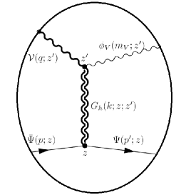
Figure 1: Witten diagram for the diffractive photoproduction of vector mesons with a bulk wave function $\phi_{V}$. The thick lines or thick wiggles represent the propagators of summed over vector meson or glueball resonances. The thin lines or thin wiggles correspond to a single vector meson and proton. For scalar glueball resonances, due to the dilaton and the trace-full part of the metric fluctuation, we simply replace the bulk-to-bulk propagator $G_{h}(k,z,z^{\prime})$ of spin-2 glueballs by $G_{\varphi,f}(k,z,z^{\prime})$.

II.2 Graviton and dilaton bulk action

Diffractive electro-production on a bulk Dirac fermion in holography, involves the exchange of tensor and scalar gravitons. The tensor graviton exchange is dual to a Reggeized tensor $2^{++}$ glueball, and the scalar graviton exchange is dual to a Reggeized scalar $0^{++}$ glueball. This is illustrated in the Witten diagram of Fig. 1. The generic effective action for these diagrams in AdS₅ is given by

$${\cal S}=\int d^{5}x\,e^{-2\phi(z)}\sqrt{g}\,{\cal L}_{EH}(g,\phi)+\int d^{5}x\,e^{-\phi(z)}\sqrt{g}\,{\cal L}_{DBI}(\psi,A,X)$$ (II.9)

with the Einstein-Hilbert action (EH) in the string frame for the metric $g$, $\phi$-dilaton, and the DBI action for the Dirac fermion $\psi$, flavor gauge field $A$, and tachyon $X$. The additional dimensionally reduced string modes, not entering the present discussion, have been omitted. The AdS₅ metric is chosen as $g_{MN}=(\eta_{\mu\nu},-1)/z^{2}$ with $\eta_{\mu\nu}$ mostly negative.

The fluctuations in the 4-dimensional part of the bulk metric, split into a transverse and traceless TT-part denoted by $h$ (tensor graviton) and a transverse and traceful T-part denoted by $f$ (scalar glueball)

$$g_{\mu\nu}(z)\rightarrow g_{\mu\nu}(z)+\sqrt{2\kappa^{2}}\bigg{[}h_{\mu\nu}(x,z)\approx\epsilon_{\mu\nu}^{TT}\,h(x,z)+\frac{1}{4}\eta_{\mu\nu}\,f(x,z)\bigg{]}$$ (II.10)

with $k^{\mu}\epsilon_{\mu\nu}^{TT}=\eta^{\mu\nu}\epsilon_{\mu\nu}^{TT}=0$. The Newtonian coupling is fixed by the D-brane tension with $16\pi G_{N}=2\kappa^{2}=8\pi^{2}/N_{c}^{2}$. The decomposition (II.10) follows in the gauge where $f,h$ decouple. However, they both obey identical equations of motion since they carry the same anomalous dimensions $\Delta_{T,S}=4$ in the strict large $N_{c}$ limit Kanitscheider:2008kd . This is not the case at finite $1/N_{c}$ (which will be subsumed below). More specifically, the radial Regge spectrum of tensor and scalar glueballs, is HILMAR

$$m_{T,S}^{2}=8\kappa_{N}^{2}\bigg{(}n+2\bigg{)}$$ (II.11)

for a background dilaton $\phi(z)=\kappa_{N}z^{2}$.

II.3 Graviton and dilaton bulk couplings

The tensor graviton and scalar dilaton coupling to the energy-momentum of the $\frac{1}{2}$ Dirac fermion and $1^{--}$ flavor vector fields in bulk is given by Mamo:2019mka

$$-\frac{\sqrt{2\kappa^{2}}}{2}\int d^{5}x\,\sqrt{g}\,h_{\mu\nu}(T_{F}^{\mu\nu}+T_{V}^{\mu\nu})=-\frac{\sqrt{2\kappa^{2}}}{2}\int d^{5}x\,\sqrt{g}\,\bigg{(}\epsilon_{\mu\nu}^{TT}\,h+\tilde{k}^{2}\frac{1}{4}\eta_{\mu\nu}\,f\bigg{)}\,(T_{F}^{\mu\nu}+T_{V}^{\mu\nu})$$ (II.12)

where the energy-momentum tensors are

$$T_{F}^{\mu\nu} = e^{-\phi_{N}}\frac{i}{2}\,z\,\overline{\Psi}\gamma^{\mu}\overset{\leftrightarrow}{\partial^{\nu}}\Psi-\eta^{\mu\nu}\mathcal{L}_{F}\,,$$

$$T_{V}^{\mu\nu} = -e^{-\phi_{V}}\Big{(}z^{4}\eta^{\rho\sigma}\eta^{\mu\beta}\eta^{\nu\gamma}\,F^{V}_{\beta\rho}F^{V}_{\gamma\sigma}-z^{4}\,\eta^{\mu\beta}\eta^{\nu\gamma}\,F^{V}_{\beta z}F^{V}_{\gamma z}\Big{)}-\eta^{\mu\nu}\mathcal{L}_{V}\,,$$ (II.13)

with $\phi_{N}=\tilde{\kappa}_{N}^{2}z^{2}$ for the nucleon field, and $\phi_{V}=\tilde{\kappa}_{V}^{2}z^{2}$ for the heavy mesons $\bar{s}\gamma^{\mu}s,\bar{c}\gamma^{\mu}c,\bar{b}\gamma^{\mu}b$ or $\phi,J/\Psi,\Upsilon$, respectively. The photon field follows from a similar reasoning with $\kappa_{V}=\kappa_{\rho}$. All vector fields are massless in bulk, since they are $p=1$ forms with anomalous dimension $\Delta_{V}=3$,

$$m^{2}_{5}=(\Delta-p)(\Delta+p-4)\rightarrow 0$$ (II.14)

Their gauge-coupling to a background tachyon field $X\sim q\bar{q}$ in bulk with a massive boundary condition $X_{0}\sim{\rm diag}(m_{u},m_{d},m_{c},m_{b})$, only generates a Higgs mass for the off-diagonal or charged flavor fields, the diagonal or neutral fields dual to $\phi,J/\Psi,\Upsilon$ remain massless in bulk. A mass $m_{c,b}$ can be added by minimally modifying the dilaton potential $\phi(z)$, without affecting the traceless condition of $T_{V}^{\mu\nu}$.

II.4 Diffractive electro-production amplitude

The scalar dilaton coupling to the flavor vector fields vanishes in bulk, i.e. $\eta_{\mu\nu}T_{V}^{\mu\nu}=0$ in (II.3), and drops out of the diffractive process in  Fig. 1 Mamo:2019mka , for both the real and virtual incoming photons. As a result, the electro-production amplitude follows solely from the exchange of a tensor glueball or graviton,

$$i{\cal A}^{h}_{\gamma^{*}p\rightarrow J/\Psi p}(s,t)\approx\frac{1}{g_{5}}\times(-i)\mathcal{V}^{\mu\nu}_{h\gamma^{*}J/\Psi}(q,q^{\prime},,k_{z})\times\bigg{(}\frac{i}{2}\eta_{\mu\alpha}\eta_{\nu\beta}\bigg{)}\times(-i)\mathcal{V}^{\alpha\beta}_{h\bar{\Psi}\Psi}(p_{1},p_{2},k_{z})\,,$$ (II.15)

with $k=p_{2}-p_{1}=q-q^{\prime}$ and

$$\mathcal{V}^{\mu\nu}_{h\gamma^{*}J/\Psi}(q,q^{\prime},k_{z})=\sqrt{2\kappa^{2}}\times\frac{1}{2}\int dz\sqrt{g}\,e^{-\phi_{J/\psi}}z^{4}K^{\mu\nu}(q,q^{\prime},\epsilon,\epsilon^{\prime},z)\frac{z^{4}}{4}\,,$$

$$\mathcal{V}_{h\bar{\Psi}\Psi}^{\alpha\beta}(p_{1},p_{2},K)=-\sqrt{2\kappa^{2}}\times\frac{1}{2}\int dz\sqrt{g}\,e^{-\phi_{N}}z\,\big{(}\psi_{R}^{2}(z)+\psi_{L}^{2}(z)\big{)}\mathcal{H}(K,z)\times\bar{u}(p_{2})\gamma^{\alpha}p^{\beta}u(p_{1})\,,$$ (II.16)

We have set $p=(p_{1}+p_{2})/2$, $q^{2}=-Q^{2}$ and $q^{\prime 2}=-Q^{\prime 2}$ for space-like momenta. The tensors are defined as

$$K^{\mu\nu}(q,q^{\prime},\epsilon,\epsilon^{\prime},z)\equiv B_{1}^{\mu\nu}\mathcal{V}_{\gamma^{*}}(Q,z)\mathcal{V}_{J/\Psi}(M_{J/\Psi},z)-B_{0}^{\mu\nu}\partial_{z}\mathcal{V}_{\gamma^{*}}(Q,z)\partial_{z}\mathcal{V}_{J/\Psi}(M_{J/\Psi},z)\,,$$ (II.17)

$$B_{0}^{\mu\nu}(\epsilon,\epsilon^{\prime})\equiv \epsilon^{\mu}\epsilon^{\prime\nu}\,,$$

$$B_{1}^{\mu\nu}(q,q^{\prime},\epsilon,\epsilon^{\prime})\equiv \epsilon\cdot\epsilon^{\prime}\,q^{\mu}q^{\prime\nu}-q\cdot\epsilon^{\prime}\,\epsilon^{\mu}q^{\prime\nu}-q^{\prime}\cdot\epsilon\,q^{\mu}\epsilon^{\prime\nu}+q\cdot q^{\prime}\,\epsilon^{\mu}\epsilon^{\prime\nu}\,.$$ (II.18)

with $B_{1,0}=\eta_{\mu\nu}B_{1,0}^{\mu\nu}$, and $K=\eta_{\mu\nu}K^{\mu\nu}$.

The non-normalizable wave function for the virtual photon $V_{\mu}(Q,z)=\mathcal{V}_{\gamma^{*}}(Q,z)\,\epsilon_{\mu}e^{-iq\cdot x}$ is the bulk-to-boundary propagator for the Reggeized process $\gamma^{*}\rightarrow c\bar{c}$

$$\mathcal{V}_{\gamma^{*}}(Q,z)=\tilde{\kappa}_{J/\Psi}^{2}z^{2}\int_{0}^{1}\frac{dx}{(1-x)^{2}}x^{a}{\rm exp}\Big{[}-\frac{x}{1-x}\tilde{\kappa}_{J/\Psi}^{2}z^{2}\Big{]}\,,$$ (II.19)

with $a={Q^{2}}/{4\tilde{\kappa}_{N}^{2}}$ and the normalization ${\cal V}_{\gamma^{*}}(0,z)={\cal V}_{\gamma^{*}}(Q,0)=1$. The normalizable wave function for $J/\Psi$ is $V_{\mu}(q^{\prime},z)=\mathcal{V}_{J/\Psi}(M_{J/\Psi},z)\,\epsilon^{\prime}_{\mu}e^{-iq^{\prime}\cdot x}$ where

$$\mathcal{V}_{J/\Psi}(M_{J/\Psi},z)=\phi_{0}(M_{J/\Psi},z)=\frac{f_{J/\Psi}}{M_{J/\Psi}}\times 2g_{5}\tilde{\kappa}_{J/\Psi}^{2}z^{2}L_{0}^{1}(\tilde{\kappa}_{J/\Psi}^{2}z^{2})\,.$$ (II.20)

The non-normalizable wave function for the virtual tansverse and traceless graviton is given by $h_{\mu\nu}(Q,z)=\mathcal{H}(Q,z)\epsilon_{\mu\nu}^{TT}e^{-iq\cdot x}$ Hong:2004sa ; CARLSON ; Abidin:2008ku ; BallonBayona:2007qr

$$\mathcal{H}(Q,z)= 4z^{4}\Gamma(a_{Q}+2)U\Big{(}a_{Q}+2,3;2\tilde{\kappa}_{N}^{2}z^{2}\Big{)}=\Gamma(a_{Q}+2)U\Big{(}a_{Q},-1;2\tilde{\kappa}_{N}^{2}z^{2}\Big{)}$$

$$= \frac{\Gamma(a_{Q}+2)}{\Gamma(a_{Q})}\int_{0}^{1}dx\,x^{a_{Q}-1}(1-x){\rm exp}\Big{(}-\frac{x}{1-x}(2\tilde{\kappa}_{N}^{2}z^{2})\Big{)}$$ (II.21)

with $a_{Q}={Q^{2}}/{8\tilde{\kappa}_{N}^{2}}$, and we have used the transformation $U(m,n;y)=y^{1-n}U(1+m-n,2-n,y)$. (II.4) satisfies the normalization condition ${\cal H}(0,z)={\cal H}(Q,0)=1$.

III Differential and total cross sections for electroproduction

III.1 Near threshold

The differential cross section for electro-production of heavy mesons $J/\Psi$ (and also $\Upsilon$) involves the exchange of a bulk $j=2$ graviton near threshold, and higher spin away from threshold. We will postpone the higher spin exchanges and their Reggeization to later.

III.1.1 $TT$ and $LL$ differential cross sections near threshold

The differential cross section for untraced in and out polarizations, near threshold, is given by (see the detailed derivations in Appendix XI)

$$\frac{d\sigma(s,t,Q,M_{J/\Psi},\epsilon_{T},\epsilon^{\prime}_{T})}{dt} = \mathcal{I}^{2}(Q,M_{J/\Psi})\times\left(\frac{s}{\tilde{\kappa}_{N}^{2}}\right)^{2}\times\mathcal{N}^{TT}(s,t,Q,M_{J/\Psi},m_{N})\times\left(-\frac{t}{4m_{N}^{2}}+1\right)\times\tilde{A}^{2}(t)\,,$$

$$\frac{d\sigma(s,t,Q,M_{J/\Psi},\epsilon_{L},\epsilon^{\prime}_{L})}{dt} = \mathcal{I}^{2}(Q,M_{J/\Psi})\times\left(\frac{s}{\tilde{\kappa}_{N}^{2}}\right)^{2}\times\frac{1}{9}\times\frac{Q^{2}}{M_{J/\Psi}^{2}}\times\mathcal{N}^{TT}(s,t,Q,M_{J/\Psi},m_{N})\times\left(-\frac{t}{4m_{N}^{2}}+1\right)\times\tilde{A}^{2}(t)\,,$$

where

$$\mathcal{I}(Q,M_{J/\Psi}) = \frac{3}{2}\frac{g_{5}f_{J/\Psi}}{M_{J/\Psi}}\times\frac{1}{\left(\frac{Q^{2}}{4\tilde{\kappa}_{J/\Psi}^{2}}+3\right)\left(\frac{Q^{2}}{4\tilde{\kappa}_{J/\Psi}^{2}}+2\right)\left(\frac{Q^{2}}{4\tilde{\kappa}_{J/\Psi}^{2}}+1\right)}$$ (III.23)

$$= \frac{3}{2}\frac{g_{5}f_{J/\Psi}}{M_{J/\Psi}}\times\tilde{\mathcal{I}}(Q,\tilde{\kappa}_{J/\Psi})\,,$$

with $\tilde{\kappa}_{J/\Psi}=\sqrt{g_{5}f_{J/\Psi}M_{J/\Psi}}/2^{3/4}$ or $g_{5}=\frac{2^{3/2}\tilde{\kappa}_{J/\Psi}^{2}}{f_{J/\Psi}M_{J/\Psi}}$, and we have defined

$$\tilde{\mathcal{I}}(Q,\tilde{\kappa}_{J/\Psi})=\frac{1}{\left(\frac{Q^{2}}{4\tilde{\kappa}_{J/\Psi}^{2}}+3\right)\left(\frac{Q^{2}}{4\tilde{\kappa}_{J/\Psi}^{2}}+2\right)\left(\frac{Q^{2}}{4\tilde{\kappa}_{J/\Psi}^{2}}+1\right)}\,.$$ (III.24)

Note that (III.23) follows from the boundary-to-bulk vector propagator that resums the $1^{--}$ $c\bar{c}$ radial Regge trajectory, in short the $1^{--}$ transition form factor $[\gamma^{*}\rightarrow c\bar{c}]+{\rm graviton}\rightarrow J/\Psi$.

The tensor form factor $A(t)$ with $t=-Q^{2}<0$, corresponds to the elastic vertex ${\rm graviton}+p\rightarrow p$. It is composed of the bulk-to-bulk graviton propagator which resums the $2^{++}$ radial Regge trajectory (III.26),

$$\tilde{A}(t)=\frac{A(t)}{A(0)} = \left(a_{K}+1\right)\left(2\left(2a_{K}^{3}+a_{K}\right)\Phi\left(-1,1,a_{K}\right)-\left(2a_{K}^{2}+a_{K}+1\right)\right)$$ (III.25)

$$= 6\times\frac{\Gamma\left(2+a_{K}\right)}{\Gamma\left(4+a_{K}\right)}\times\,_{2}F_{1}\left(3,a_{K};a_{K}+4;-1\right)$$

$$= \bigg{(}(1-2a_{K})(1+a_{K}^{2})+a_{K}(1+a_{K})(1+2a_{K}^{2})\bigg{(}H\bigg{(}\frac{1+a_{K}}{2}\bigg{)}-H\bigg{(}\frac{a_{K}}{2}\bigg{)}\bigg{)}\bigg{)}$$

with $a_{K}={-t}/{8\tilde{\kappa}_{N}^{2}}$. $H(x)=\psi(1+x)+\gamma$ is the harmonic number or the di-gamma function plus Euler number. We fix $\tilde{\kappa}_{N}=0.350$ GeV to reproduce both the nucleon ${\frac{1}{2}}^{+}$ and the $1^{--}$ rho radial Regge trajectories

$$m_{N}^{2}(n)=4\tilde{\kappa}^{2}_{N}(n+\tau_{N}-1)=4\tilde{\kappa}^{2}_{N}(n+2)\qquad\qquad m_{\rho}^{2}(n)=4\tilde{\kappa}^{2}_{N}\bigg{(}n+\frac{\Delta_{\rho}-p}{2}\bigg{)}=4\tilde{\kappa}^{2}_{N}(n+1)$$ (III.26)

with $m_{N}(0)\approx 990$ MeV and $m_{\rho}(0)\approx 700$ MeV, and $\tau_{N}=3$ to reproduce the hard scattering rules. With this in mind, (III.25) is well parametrized by a dipole

$$\tilde{A}(t)=\frac{A(t)}{A(0)}\approx\frac{1}{\left(1-\frac{t}{1.124^{2}}\right)^{2}}\,.$$ (III.27)

From (III.25) the mass radius of the proton from the exchange of a tensor glueball is

$$\langle r^{2}_{Mass}\rangle=6\bigg{(}\frac{d{\rm ln}A(t)}{dt}\bigg{)}_{0}=\frac{1.04}{{\tilde{\kappa}}_{N}^{2}}=(0.57\,{\rm fm})^{2}$$ (III.28)

A slightly improved assessment of the mass radius can be achieved by fixing $\tilde{\kappa}_{N}$ using the physical rho mass in (III.26), and a smaller nucleon twist factor $\tau_{N}=3\rightarrow 2.465$ by using the nucleon mass as in our recent charge radii re-analyses in Mamo:2021jhj . This will not be pursued here, to keep the present electro-production analysis in line with our photon-production analysis in Mamo:2019mka for comparison.

The transverse $TT$ and longitudinal $LL$ normalizations, for heavy mesons, are defined as (assuming $s\sim s_{th}\gg m_{N}^{2},Q^{2},M_{V}^{2}$, and $|t|\ll s_{th}$ in (XI))

$$\mathcal{N}^{TT}(s,t,Q,M_{J/\Psi},m_{N}) = \frac{e^{2}\times\frac{(2\kappa^{2})^{2}}{g_{5}^{2}}}{16\pi}\,\frac{1}{2}\times\frac{\tilde{\kappa}_{N}^{4}}{\tilde{\kappa}_{J/\Psi}^{8}}\times A^{2}(0)\times\frac{1}{16}\times 8=constant\,,$$

$$\mathcal{N}^{LL}(s,t,Q,M_{J/\Psi},m_{N}) = \mathcal{N}^{TT}(s,t,Q,M_{J/\Psi},m_{N})\,,$$

where we used $\frac{1}{s^{4}}\tilde{F}(s)=\frac{1}{16}$ in (XI).

III.1.2 $TT+LL$ differential cross section near threshold

The total differential cross section

$$\left(\frac{d\sigma}{dt}\right)_{{\rm tot}}=\frac{d\sigma(s,t,Q,M_{J/\Psi},\epsilon_{T},\epsilon^{\prime}_{T})}{dt}+\frac{d\sigma(s,t,Q,M_{J/\Psi},\epsilon_{L},\epsilon^{\prime}_{L})}{dt}\,,$$ (III.30)

is the sum of the transverse and longitudinal contributions, which takes the explicit form

$$\left(\frac{d\sigma}{dt}\right)_{{\rm tot}}=\mathcal{N}_{t}(s,Q;{\mathbb{\tilde{N}}}^{\prime})\times\Big{(}-\frac{t^{2}}{4m_{N}^{2}}+1\Big{)}\times\tilde{A}^{2}(t)\,,$$ (III.31)

The overall normalization in (III.31)

$$\mathcal{N}_{t}(s,Q;\mathbb{\tilde{N}}^{\prime}) \equiv \mathcal{I}^{2}(Q,M_{J/\Psi})\times\left(\frac{s}{\tilde{\kappa}_{N}^{2}}\right)^{2}\times\mathcal{N}^{TT}(s,t,Q,M_{J/\Psi},m_{N})$$ (III.32)

$$\times \left(1+\mathcal{\tilde{N}}_{R}^{2}\times\frac{1}{9}\times\frac{Q^{2}}{M_{J/\Psi}^{2}}\right)\times\mathbb{\tilde{N}}^{\prime}\,,$$

is fixed by our preceding arguments. Strict bulk-to-boundary correspondence implies $\mathbb{\tilde{N}}^{\prime}=1$ and $\mathcal{\tilde{N}}_{R}=1$ in the double limit of large $N_{c}$ and strong gauge coupling $\lambda$. Here we assume proportionality between the bulk and boundary with $\mathbb{\tilde{N}}^{\prime}$ and $\mathcal{\tilde{N}}_{R}$ overall parameters that captures the finite $N_{c}$ corrections. They will be fixed by the best fit to the data below.

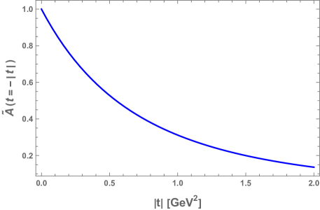
Figure 2: The spin-2 nucleon gravitational form factor $\tilde{A}(t=-|t|)$ given in (III.25).

III.1.3 Total cross section near threshold

The total cross section for electro-production of a vector meson follows from the differential cross section by integrating the differential cross section from $t_{min}$ to $t_{max}$, i.e.,

$$\sigma_{tot}(s,Q^{2})=\int_{t_{min}}^{t_{max}}\,dt\left(\frac{d\sigma}{dt}\right)_{{\rm tot}}\,,$$ (III.33)

where

$$\left(\frac{d\sigma}{dt}\right)_{{\rm tot}}=\frac{d\sigma(s,t,Q,M_{J/\Psi},\epsilon_{T},\epsilon^{\prime}_{T})}{dt}+\frac{d\sigma(s,t,Q,M_{J/\Psi},\epsilon_{L},\epsilon^{\prime}_{L})}{dt}\,,$$ (III.34)

and, $t_{min}\equiv|t|_{\cos\theta=+1}|$ and $t_{max}\equiv|t|_{\cos\theta=-1}|$ with $t$ given by (VIII), see also Fig. 12.

We can also define

$$\sigma_{T}(s,Q^{2})=\int_{t_{min}}^{t_{max}}\,dt\frac{d\sigma(s,t,Q,M_{J/\Psi},\epsilon_{T},\epsilon^{\prime}_{T})}{dt}\,,$$ (III.35)

and

$$\sigma_{L}(s,Q^{2})=\int_{t_{min}}^{t_{max}}\,dt\frac{d\sigma(s,t,Q,M_{J/\Psi},\epsilon_{L},\epsilon^{\prime}_{L})}{dt}\,.$$ (III.36)

A more explicit form of the total cross section (III.33) is

$$\sigma_{tot}(s,Q^{2})=\mathcal{N}_{Q^{2}}(s,f_{J/\Psi},M_{J/\Psi};\mathbb{\tilde{N}})\times\mathcal{\tilde{I}}(Q,\tilde{\kappa}_{J/\Psi})\times\left(1+\mathcal{\tilde{N}}_{R}^{2}\times\frac{1}{9}\times\frac{Q^{2}}{M_{J/\Psi}^{2}}\right)\,,$$

where $\mathcal{\tilde{I}}(Q,\tilde{\kappa}_{J/\Psi})$ is given by (III.24), and we have defined

$$\mathcal{N}_{Q^{2}}(s,f_{J/\Psi},M_{J/\Psi};\mathbb{\tilde{N}})\equiv\mathcal{N}^{TT}(s,t,Q,M_{J/\Psi},m_{N})\times\frac{3}{2}\frac{g_{5}f_{J/\Psi}}{M_{J/\Psi}}\times\mathbb{\tilde{N}}\times\left(\frac{s}{\tilde{\kappa}_{N}^{2}}\right)^{2}\times\int_{t_{min}}^{t_{max}}d|t|\,\left(\frac{|t|}{4m_{N}^{2}}+1\right)\times\tilde{A}^{2}(t=-|t|)\,.$$

Again, we assume proportionality between the bulk and boundary with $\mathbb{\tilde{N}}$ and $\mathcal{\tilde{N}}_{R}$ overall parameters that capture the finite $N_{c}$ corrections. They will be fixed by the best fit to the data below. Also note that $\mathcal{N}^{TT}(s,t,Q,M_{J/\Psi},m_{N})$ is given by (III.1.1), and it is a constant independent of $Q$, $t$ and $s$.

III.2 Far from threshold

The differential cross sections (III.1.1) grow as $s^{2}$ following the exchange of spin $j=2$ as a tensor glueball in bulk. At larger $\sqrt{s}$ higher spin-j exchanges contribute. Their resummation Reggeizes leading to a soft Pomeron exchange. This transmutation from a graviton to a Pomeron was initially discussed in Brower:2006ea . In this section we apply this resummation to the electro-production process.

III.2.1 $TT$ and $LL$ differential cross sections far from threshold

More specifically, the differential cross section for the untraced in and out polarizations, in the high energy regime, is given by (see the detailed derivations in Appendix XII)

$$\frac{d\sigma(s,t,Q,M_{J/\Psi},\epsilon_{T},\epsilon^{\prime}_{T})}{dt} = \mathcal{I}^{2}(j_{0},Q,M_{J/\Psi})\times\left(\frac{s}{\tilde{\kappa}_{N}^{2}}\right)^{2\left(1-\frac{2}{\sqrt{\lambda}}\right)}\times\mathcal{N}^{TT}(j_{0},s,t,Q,M_{J/\Psi},m_{N})\times\mathcal{A}^{2}(j_{0},\tau,\Delta,t)\,,$$

$$\frac{d\sigma(s,t,Q,M_{J/\Psi},\epsilon_{L},\epsilon^{\prime}_{L})}{dt} = \mathcal{I}^{2}(j_{0},Q,M_{J/\Psi})\times\left(\frac{s}{\tilde{\kappa}_{N}^{2}}\right)^{2\left(1-\frac{2}{\sqrt{\lambda}}\right)}\times\mathcal{N}^{LL}(j_{0},s,t,Q,M_{J/\Psi},m_{N})\times\mathcal{A}^{2}(j_{0},\tau,\Delta,t)\,.$$

The $TT$ and $LL$ normalizations in (III.2.1) are purely kinematical in origin

$$\mathcal{N}^{TT}(j_{0},s,t,Q,M_{J/\Psi},m_{N}) = \frac{e^{2}\times\frac{(2\kappa^{2})^{2}}{g_{5}^{2}}}{16\pi}\,\frac{1}{2}\times P(\tilde{s},\lambda)\times\frac{\tilde{\kappa}_{N}^{4}}{\tilde{\kappa}_{J/\Psi}^{8}}\times\Bigg{(}\frac{\tilde{\kappa}_{N}^{2}}{\tilde{\kappa}_{J/\Psi}^{2}}\Bigg{)}^{-2\big{(}1+\frac{1}{\sqrt{\lambda}}\big{)}}\times A^{2}(0)\times\frac{1}{s^{4}}\tilde{F}(s)\times 8$$

$$\mathcal{N}^{LL}(j_{0},s,t,Q,M_{J/\Psi},m_{N}) = \left(\frac{1}{2-\frac{1}{\sqrt{\lambda}}}\right)^{2}\times\frac{Q^{2}}{M_{J/\Psi}^{2}}\times\mathcal{N}^{TT}(j_{0},s,t,Q,M_{J/\Psi},m_{N})\,,$$ (III.40)

with

$$\tilde{F}(s)=\frac{1}{16}\times s^{4}\,,$$ (III.41)

and

$$P(\tilde{s},\lambda) \equiv \left[\lambda/\pi^{2}+1\right](\sqrt{\lambda}/2\pi)\;\tilde{\xi}^{2}\;\frac{e^{-2\sqrt{\lambda}\tilde{\xi}^{2}/2\tilde{\tau}}}{\tilde{\tau}^{3}}\left(1+{\cal O}\bigg{(}\frac{\sqrt{\lambda}}{\tilde{\tau}}\bigg{)}\right)\,,$$ (III.42)

where $\tilde{\tau}\equiv\log\tilde{s}=\log[s/\tilde{\kappa}_{N}^{2}]$ and $\tilde{\xi}-\pi/2=\gamma=0.55772.....$ is Euler-Mascheroni constant.

The transition form factor for $\gamma^{*}+\mathbb{P}\rightarrow J/\Psi$ is

$$\mathcal{I}(j_{0},Q,M_{J/\Psi}) = \frac{1}{2}\frac{g_{5}f_{J/\Psi}}{M_{J/\Psi}}\times\frac{\Gamma\left(\frac{Q^{2}}{4\tilde{\kappa}_{J/\Psi}^{2}}+1\right)}{\Gamma\left(\frac{Q^{2}}{4\tilde{\kappa}_{J/\Psi}^{2}}+1-\frac{1}{\sqrt{\lambda}}\right)}\times\left(2-\frac{1}{\sqrt{\lambda}}\right)\times\frac{1}{4}\Gamma^{2}\left(2-\frac{1}{\sqrt{\lambda}}\right)$$

$$\times \frac{1}{\left(\frac{Q^{2}}{4\tilde{\kappa}_{J/\Psi}^{2}}+2-\frac{1}{\sqrt{\lambda}}\right)\left(\frac{Q^{2}}{4\tilde{\kappa}_{J/\Psi}^{2}}+1-\frac{1}{\sqrt{\lambda}}\right)}\,,$$

$$= \frac{1}{2}\frac{g_{5}f_{J/\Psi}}{M_{J/\Psi}}\times\left(2-\frac{1}{\sqrt{\lambda}}\right)\times\frac{1}{4}\Gamma^{2}\left(2-\frac{1}{\sqrt{\lambda}}\right)\times\mathcal{\tilde{I}}(\lambda,Q,\tilde{\kappa}_{J/\Psi})$$

with

$$\mathcal{\tilde{I}}(\lambda,Q,\tilde{\kappa}_{J/\Psi})\equiv\frac{\Gamma\left(\frac{Q^{2}}{4\tilde{\kappa}_{J/\Psi}^{2}}+1\right)/\Gamma\left(\frac{Q^{2}}{4\tilde{\kappa}_{J/\Psi}^{2}}-\frac{1}{\sqrt{\lambda}}\right)}{\left(\frac{Q^{2}}{4\tilde{\kappa}_{J/\Psi}^{2}}-\frac{1}{\sqrt{\lambda}}\right)\left(\frac{Q^{2}}{4\tilde{\kappa}_{J/\Psi}^{2}}+2-\frac{1}{\sqrt{\lambda}}\right)\left(\frac{Q^{2}}{4\tilde{\kappa}_{J/\Psi}^{2}}+1-\frac{1}{\sqrt{\lambda}}\right)}\,,$$ (III.44)

with $\tilde{\kappa}_{J/\Psi}=2^{-3/4}\sqrt{g_{5}f_{J/\Psi}M_{J/\Psi}}$, which Reggeizes the $1^{--}$ trajectory, with a substantial fall-off at large $Q^{2}$.

III.2.2 $TT+LL$ differential cross section far from threshold

The total differential cross section

$$\left(\frac{d\sigma}{dt}\right)_{{\rm tot}}=\frac{d\sigma(s,t,Q,M_{J/\Psi},\epsilon_{T},\epsilon^{\prime}_{T})}{dt}+\frac{d\sigma(s,t,Q,M_{J/\Psi},\epsilon_{L},\epsilon^{\prime}_{L})}{dt}\,,$$ (III.45)

is the sum of the transverse and longitudinal contributions, which takes the explicit form

$$\left(\frac{d\sigma}{dt}\right)_{{\rm tot}}=\mathcal{N}_{t}(s,Q;{\mathbb{N}}^{\prime})\times\Big{(}-\frac{t^{2}}{4m_{N}^{2}}+1\Big{)}\times\mathcal{A}^{2}(j_{0},\tau,\Delta,t)\,,$$ (III.46)

The overall normalization in (III.46)

$$\mathcal{N}_{t}(s,Q;\mathbb{N}^{\prime}) \equiv \mathcal{I}^{2}(j_{0},Q,M_{J/\Psi})\times\left(\frac{s}{\tilde{\kappa}_{N}^{2}}\right)^{2-\frac{4}{\sqrt{\lambda}}}\times\mathcal{N}^{TT}(j_{0},s,t,Q,M_{J/\Psi},m_{N})$$ (III.47)

$$\times \left(1+\mathcal{N}_{R}^{2}\times\left(\frac{1}{2-\frac{1}{\sqrt{\lambda}}}\right)^{2}\times\frac{Q^{2}}{M_{J/\Psi}^{2}}\right)\times\mathbb{N}^{\prime}\,,$$

is fixed by our preceding arguments. Strict bulk-to-boundary correspondence implies $\mathbb{N}^{\prime}=1$ and $\mathcal{N}_{R}=1$ in the double limit of large $N_{c}$ and strong gauge coupling $\lambda$. Here we assume proportionality between the bulk and boundary with $\mathbb{N}^{\prime}$ and $\mathcal{N}_{R}=1$ overall parameters that capture the finite $N_{c}$ corrections. They will be fixed by the best fit to the data below.

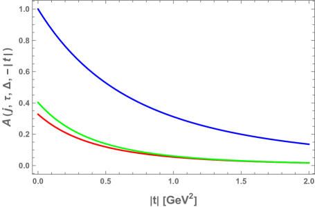
Figure 3: The spin-j nucleon form factor ${\cal A}(j,\tau,\Delta(j),t=-|t|)$: Upper-blue-curve is $j=j_{0}=2$ and $\Delta(j=2)=4$ in (III.2.2); Middle-green curve is $j=j_{0}=2-2/\sqrt{\lambda}$ and $\Delta(j=j_{0})=2$ with $\sqrt{\lambda}=\infty$ in (III.2.2); Lower-red-curve is $j=j_{0}=2-2/\sqrt{\lambda}$ and $\Delta(j=j_{0})=2$ with $\sqrt{\lambda}=\sqrt{11.243}$ in (III.2.2).

$\mathcal{A}(j_{0},\tau,\Delta,t)$ is the Pomeron-nucleon form factor ${\mathbb{P}}+p\rightarrow p$

$$\mathcal{A}(j=j_{0},\tau,\Delta,t)=\Gamma\left(a_{K}+\frac{\Delta(j)}{2}\right)$$

$$\times \frac{2^{1-\Delta}}{\Gamma(\tau)}\Bigg{(}(\tau-1)\Gamma\left(\frac{j}{2}+\tau-\frac{\Delta}{2}\right)\Gamma\left(\frac{1}{2}(j+\Delta+2\tau-4)\right)\,_{2}F_{1}\left(\frac{1}{2}(j-\Delta+2\tau),\frac{1}{2}\left(-\Delta+2a_{k}+4\right);\frac{1}{2}\left(j+2\tau+2a_{k}\right);-1\right)$$

$$+ \Gamma\left(\frac{j}{2}+\tau-\frac{\Delta}{2}+1\right)\Gamma\left(\frac{1}{2}(j+\Delta+2\tau-2)\right)\,_{2}F_{1}\left(\frac{1}{2}(j-\Delta+2\tau+2),\frac{1}{2}\left(-\Delta+2a_{k}+4\right);\frac{1}{2}\left(j+2\tau+2a_{k}+2\right);-1\right)\Bigg{)}\,,$$

with the proton twist $\tau=3$ (fixed by the hard counting rule of the proton electromagnetic form factor), $j_{0}=2-\frac{2}{\sqrt{\lambda}}$, $\Delta(j=j_{0})=2$, and $a_{K}={K^{2}}/{8\tilde{\kappa}_{N}^{2}}={-t}/{8\tilde{\kappa}_{N}^{2}}$ at $\tilde{\kappa}_{N}=0.350~{}GeV$ (fixed by the mass of the rho meson and proton). (III.2.2) controls the t-dependence in the high energy regime $\sqrt{s}\gg\sqrt{|t|}$.

In Fig. 3 we show the spin-j nucleon form factor ${\cal A}(j,\tau,\Delta(j),t=-|t|)$ versus $t$. The red-curve is the spin-$j_{0}$ nucleon form factor or Pomeron-nucleon form factor ${\cal A}(j=j_{0},\tau=3,\Delta(j=j_{0})=2,t=-|t|)$ with $j_{0}=2-2/\sqrt{\lambda}$ and $\sqrt{\lambda}=\sqrt{11.243}$ in (III.2.2).The corresponding mass radius squared is $(0.425~{}\rm fm)^{2}$. The green-curve is the spin-$j_{0}$ nucleon form factor or the Pomeron-nucleon form factor ${\cal A}(j=j_{0},\tau=3,\Delta(j=j_{0})=2,t=-|t|)$ with $j_{0}=2-2/\sqrt{\lambda}$ and $\sqrt{\lambda}=\infty$ in (III.2.2). The corresponding mass radius squared is $(0.482~{}\rm fm)^{2}$. The blue-curve is the spin-$2$ nucleon form factor or the gravitational spin-2 form factor ${\cal A}(j=2,\tau=3,\Delta(j=2)=4,t=-|t|)=\tilde{A}(t=-|t|)$ in (III.2.2) with mass radius squared of $(0.575~{}\rm fm)^{2}$  Mamo:2019mka ; Mamo:2021krl . The resummed spin-j gluonic sourced by the nucleon is more compact with a heavier tail.

III.2.3 Total cross section far from threshold

The total cross section for electro-production of a vector meson follows from the differential cross section using the optical theorem

$$\sigma_{tot}(s,Q^{2})=\bigg{(}\frac{16\pi}{1+\rho^{2}}\left(\frac{d\sigma}{dt}\right)_{{\rm tot}}\bigg{)}_{t=0}^{\frac{1}{2}}$$ (III.49)

with the rho-parameter

$$\rho=\frac{\text{Re}[{\cal A}^{tot}_{\gamma*p\rightarrow J/\Psi p}(s,t=0)]}{\text{Im}[{\cal A}^{tot}_{\gamma*p\rightarrow J/\Psi p}(s,t=0)]}\simeq\frac{\sqrt{\lambda}}{\pi}\,.$$ (III.50)

The cross sections for transversely and longitudinally polarized processes are

$$\sigma_{T}(s,Q^{2})= \bigg{(}\frac{16\pi}{1+\rho^{2}}\frac{d\sigma(s,t,Q,M_{J/\Psi},\epsilon_{T},\epsilon^{\prime}_{T})}{dt}\bigg{)}_{t=0}^{\frac{1}{2}}\,,$$

$$\sigma_{L}(s,Q^{2})= \bigg{(}\frac{16\pi}{1+\rho^{2}}\frac{d\sigma(s,t,Q,M_{J/\Psi},\epsilon_{L},\epsilon^{\prime}_{L})}{dt}\bigg{)}_{t=0}^{\frac{1}{2}}\,.$$ (III.51)

A more explicit form of the total cross section (III.49) is

$$\sigma_{tot}(s,Q^{2})=\mathcal{N}_{Q^{2}}(s,\lambda,f_{J/\Psi},M_{J/\Psi};\mathbb{N})\times\mathcal{\tilde{I}}(\lambda,Q,\tilde{\kappa}_{J/\Psi})\times\left(1+\mathcal{N}_{R}^{2}\times\left(\frac{1}{2-\frac{1}{\sqrt{\lambda}}}\right)^{2}\times\frac{Q^{2}}{M_{J/\Psi}^{2}}\right)^{1/2}\,,$$

where $\mathcal{\tilde{I}}(\lambda,Q,\tilde{\kappa}_{J/\Psi})$ is given by (III.44), and we have defined

$$\mathcal{N}_{Q^{2}}(s,\lambda,f_{J/\Psi},M_{J/\Psi};\mathbb{N}) \equiv \bigg{(}{\frac{16\pi}{1+\rho^{2}}}\bigg{)}^{\frac{1}{2}}\times\bigg{(}{\left(\frac{s}{\tilde{\kappa}_{N}^{2}}\right)^{2-\frac{4}{\sqrt{\lambda}}}\times\mathcal{N}^{TT}(j_{0},s,t=0,Q,M_{J/\Psi},m_{N})\times\mathcal{A}^{2}(j_{0},\tau,\Delta,t=0)}\bigg{)}^{\frac{1}{2}}$$ (III.53)

$$\times \frac{1}{2}\frac{g_{5}f_{J/\Psi}}{M_{J/\Psi}}\times\left(2-\frac{1}{\sqrt{\lambda}}\right)\times\frac{1}{4}\Gamma^{2}\left(2-\frac{1}{\sqrt{\lambda}}\right)\times\mathbb{N}\,,$$

Again, we assume proportionality between the bulk and boundary with $\mathbb{N}$ and $\mathcal{N}_{R}$ overall parameters that capture the finite $N_{c}$ corrections. They will be fixed by the best fit to the data below.

IV Results for near threshold

For quasi-real electroproduction ($Q^{2}\ll\frac{9}{\mathcal{\tilde{N}}_{R}}\times M_{J/\Psi}^{2}$), we can approximate the normalization (III.32) as

$$\mathcal{N}_{t}(s,Q;\mathbb{\tilde{N}}^{\prime}) \equiv \mathcal{I}^{2}(Q,M_{J/\Psi})\times\left(\frac{s}{\tilde{\kappa}_{N}^{2}}\right)^{2}\times\mathcal{N}^{TT}(s,t,Q,M_{J/\Psi},m_{N})$$ (IV.54)

$$\times \left(1+\mathcal{\tilde{N}}_{R}^{2}\times\frac{1}{9}\times\frac{Q^{2}}{M_{J/\Psi}^{2}}\right)\times\mathbb{\tilde{N}}^{\prime}\,.$$

In Fig. 4 we show our prediction for the variation of the total differential cross section with $Q^{2}$ (III.31) and fixed $\sqrt{s}=\sqrt{2}1~{}\text{GeV}$, in the quasi-real electro-production regime near threshold ($Q^{2}\ll\frac{9}{\mathcal{\tilde{N}}_{R}}\times M_{V}^{2}$), using the normalization (IV.54). We have fixed the $J/\Psi$ parameters as follows: $M_{J/\Psi}=3.1~{}\text{GeV}$, $f_{J/\Psi}=0.405~{}\text{GeV}$, $\tilde{\kappa}_{J/\Psi}=1.03784~{}\text{GeV}$ (using the high energy electro-production data for $J/\Psi$ as discussed in the next section), and $A^{2}(0)\times\mathbb{\tilde{N}}^{\prime}=30.7944~{}[\text{nb}/\text{GeV}^{2}]$. The upper-blue-curve is for $Q=0$. The middle-red-curve is for $Q=1.2~{}\text{GeV}$. The lower-green-curve is for $Q=2.2~{}\text{GeV}$. The dashed-purple-lines are the total differential cross sections using our kinematic factors using the lattice dipole gravitational form factor with $m_{A}=1.13~{}\rm GeV$ MIT . The data for $Q=0$ is from the GlueX collaboration GLUEX . With increasing $Q$, the differential cross section becomes less sensitive to $|t|$ in the treshold region.

In Fig. 5 we show the total cross section at the photon-point with $Q^{2}=0$ for $J/\Psi$ photo-production, by fixing $A^{2}(0)\times\mathbb{\tilde{N}}=240\pm 47$ and $\tilde{\kappa}_{J/\Psi}=1.03784$ (using the high energy electro-production data for $J/\Psi$ as discussed in the next section). The $J/\Psi$ parameters are fixed as before, with $e=0.3$, $\tilde{\kappa}_{N}=0.350~{}\text{GeV}$ and $m_{N}=0.94~{}\text{GeV}$. The data are from GlueX GLUEX .

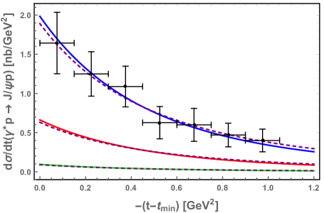
Figure 4: The total differential cross section (III.31) normalized using (IV.54) for $\sqrt{s}=\sqrt{2}1~{}\text{GeV}$. The upper-blue-curve is for $Q=0$, the middle-red-curve is for $Q=1.2~{}\text{GeV}$, and the lower-green-curve is for $Q=2.2~{}\text{GeV}$. The purple-dashed-curves are our results using the lattice dipole gravitational form factor with $m_{A}=1.13~{}\rm GeV$ MIT . The data is from the GlueX collaboration at JLab GLUEX .

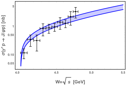
Figure 5: Total holographic cross section (III.1.3) for photo-production of $J/\Psi$ versus the GlueX data GLUEX . See text.

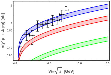
Figure 6: The total cross section (IV.55) for $\tilde{\kappa}_{N}=0.350~{}\text{GeV},e=0.3,f_{J/\Psi}=0.405~{}\text{GeV},M_{J/\Psi}=3.1~{}\text{GeV},A^{2}(0)\times\mathbb{\tilde{N}}=240\pm 47,\tilde{\kappa}_{J/\Psi}=1.03784~{}\text{GeV}$. The blue band is for $Q^{2}=0$ (the data is from GlueX (GLUEX )), the red band is for $Q^{2}=1.2^{2}~{}\text{GeV}^{2}$, the green band is for $Q^{2}=2.2^{2}~{}\text{GeV}^{2}$.

For quasi-real electro-production ($Q^{2}\ll\frac{9}{\mathcal{\tilde{N}}_{R}}\times M_{J/\Psi}^{2}$), we can approximate the total cross section (III.1.3) as

$$\sigma_{tot}(s,Q^{2})\approx\mathcal{\tilde{N}}_{Q^{2}}(s,f_{J/\Psi},M_{J/\Psi};n)\times\mathcal{\tilde{I}}^{2}(Q,\tilde{\kappa}_{J/\Psi})\,,$$ (IV.55)

In Fig. 6 we show (IV.55) versus $\sqrt{s}$ for $Q^{2}=0$ in upper-blue-filled-band, for $Q^{2}=1.2^{2}~{}\text{GeV}^{2}$ middle-red-filled-band, and $Q^{2}=2.2^{2}~{}\text{GeV}^{2}$ lower-green-filled-band. The data is from GlueX GLUEX . In Fig. 7 we show the total cross section (IV.55) versus $Q^{2}$ for fixed $W=\sqrt{s}=4.4~{}\text{GeV}$. Again, we have fixed the $J/\Psi$ parameters as: $e=0.3,f_{J/\Psi}=0.405~{}\text{GeV}$, $M_{J/\Psi}=3.1~{}\text{GeV}$ and $\tilde{\kappa}_{J/\Psi}=1.03784~{}\text{GeV}$. The bands follow from the range in the choice of the overall normalization $A^{2}(0)\times\tilde{n}=240\pm 47$.

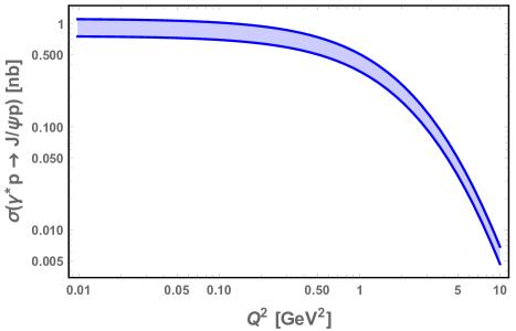
Figure 7: The total cross section for quasi-real electro-production of $J/\Psi$ in (IV.55) versus $Q^{2}$ for fixed $W=\sqrt{s}=4.4~{}\text{GeV}$. See text.

V Results far from threshold

V.1 $J/\Psi$ electro-production

In the $J/\Psi$ electro-production channel, we fix the ^′t Hooft coupling $\lambda=11.243$ and $\tilde{\kappa}_{J/\Psi}=1.03784~{}\text{GeV}$, for a mass $M_{J/\Psi}=3.1$ GeV and a decay constant $f_{J/\Psi}=0.405$ GeV. In Fig. 8 we show the $Q^{2}$ dependence of the ratio of the longitudinal to transverse cross sections as in (III.2.3)

$$R=\frac{\sigma_{L}}{\sigma_{R}}=\mathcal{N}_{R}\times\left(\frac{1}{2-\frac{1}{\sqrt{11.243}}}\right)\times\frac{Q}{3.1~{}\text{GeV}}$$ (V.56)

The overall and arbitrary normalization is ${\cal N}_{R}=0.6$ for the blue-solid curve. The data are from the 2005 H1 collaboration at HERA Aktas:2005xu . The slow rise in the semi-logarithmic plot is consistent with the linear Q-behavior following from holography, since $d\sigma_{L}/dt\sim 1/Q^{6}$ and $d\sigma_{T}/dt\sim 1/Q^{8}$. Asymptotically, the effective size is fixed by the virtual photon size $1/Q$.

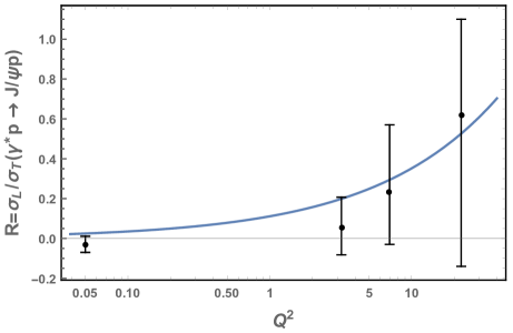
Figure 8: Ratio $R=\sigma_{L}/\sigma_{T}$ of the total longitudinal to transverse cross sections versus $Q^{2}$ for $J/\Psi$ electro-production as given in (V.56).

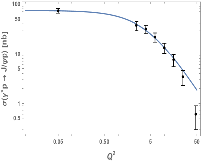
(a)

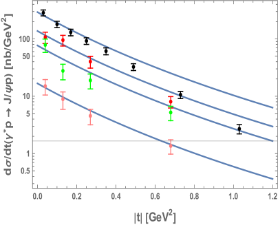
(b)

Figure 9: a: the blue-solid line is the total $J/\Psi$ electro-production cross section versus $Q^{2}$ for fixed $\sqrt{s}=90$ GeV, in comparison to the HERA data Aktas:2005xu ; (b): the blue-solid lines are the differential $J/\Psi$ electro-production cross section versus $|t|$, for $40\,{\rm GeV}<\sqrt{s}<160\,{\rm GeV}$ in comparison to the HERA data Aktas:2005xu . The black-data points are for $Q=\sqrt{0.05}\,{\rm GeV}$, the red-data points are for $Q=\sqrt{3.2}\,{\rm GeV}$, the green-data points are for $Q=\sqrt{7}\,{\rm GeV}$, the pink-data points are for $Q=\sqrt{22.4}\,{\rm GeV}$.

In Fig. 9a, we show the total holographic cross section for the electro-production of $J/\Psi$ as given in (III.2.3) versus $Q^{2}$ and for fixed $\sqrt{s}=90$ GeV,

$$\sigma_{tot}(Q^{2})=\mathcal{N}_{Q^{2}}\times\mathcal{\tilde{I}}(\lambda=11.243,Q,\tilde{\kappa}_{J/\Psi}=1.03784~{}\text{GeV})\times\left(1+0.6^{2}\times\left(\frac{1}{2-\frac{1}{\sqrt{11.243}}}\right)^{2}\times\frac{Q^{2}}{3.1^{2}~{}\text{GeV}^{2}}\right)^{1/2}$$ (V.57)

with the form factor $\mathcal{\tilde{I}}(\lambda,Q,\tilde{\kappa}_{J/\Psi})$ given in (III.44), $\lambda=11.243,f_{J/\Psi}=0.405~{}\text{GeV},M_{J/\Psi}=3.1~{}\text{GeV},A^{2}(0)\times{\mathbb{N}}=206,556~{}[nb]$, $\mathcal{N}_{R}=0.6$, and $\tilde{\kappa}_{J/\Psi}=1.03784~{}\text{GeV}$. The holographic cross section is in agreement with the reported data in the range $0\leq Q^{2}\leq 10\,{\rm GeV}^{2}$. This is expected since at higher $Q^{2}$ the weak coupling regime sets in. This observation is consistent with our recent analysis of neutrino-nucleon DIS scattering in holographic QCD Mamo:2021cle . Fig. 9a shows that the holographic $Q^{2}$ dependence following from $\tilde{\cal{I}}$ is consistent with the data at low and intermediate values of $Q^{2}$. This dependence originates from the bulk-to-boundary vector propagator (III.23) which re-sums the $c\bar{c}$ radial Regge trajectory.

In Fig. 9b we show the differential cross section (III.46) for the electro-production of $J/\Psi$, after adjusting the overall matching parameter $\mathbb{N}^{\prime}$ to a data point, as follows

$$40^{2}~{}{\rm GeV}^{2}<s<160^{2}~{}{\rm GeV}^{2},Q=\sqrt{0.05}~{}{\rm GeV},A^{2}(0)\times{\mathbb{N}}^{\prime}=9.33\times 10^{13}~{}[nb/GeV^{2}]\qquad{\rm black-data},$$

$$40^{2}~{}{\rm GeV}^{2}<s<160^{2}~{}{\rm GeV}^{2},Q=\sqrt{3.2}~{}{\rm GeV},A^{2}(0)\times{\mathbb{N}}^{\prime}=1.98\times 10^{14}~{}[nb/GeV^{2}]\qquad\,\,\,{\rm red-data},$$

$$40^{2}~{}{\rm GeV}^{2}<s<160^{2}~{}{\rm GeV}^{2},Q=\sqrt{7}~{}{\rm GeV},A^{2}(0)\times{\mathbb{N}}^{\prime}=3.62\times 10^{14}~{}[nb/GeV^{2}]\qquad\,\,\,\,\,\,\,{\rm green-data},$$

$$40^{2}~{}{\rm GeV}^{2}<s<160^{2}~{}{\rm GeV}^{2},Q=\sqrt{22.4}~{}{\rm GeV},A^{2}(0)\times{\mathbb{N}}^{\prime}=1.01\times 10^{15}~{}[nb/GeV^{2}]\qquad{\rm pink-data}.$$

The data are from the 2005 H1 collaboration at HERA in Aktas:2005xu . The $|t|$ dependence of the holographic differential cross sections follow from $|{\cal A}(j_{0},\tau,\Delta,t)|^{2}$ as given in (III.2.2), and is consistent with the reported data for $J/\Psi$ electro-production at HERA for different $Q^{2}$. Recall that in the threshold region with $\sqrt{s}\sim(m_{N}+m_{J/\Psi})$, ${\cal A}(2,3,4,t)=A(t)$ in (III.25) which is the gravitational tensor coupling. Its Reggeized form ${\cal A}(j_{0},\tau,\Delta,t)$ is probed by the differential cross section of $J/\Psi$ electro-production at large $\sqrt{s}$.

V.2 $\phi$ electro-production

Although most of our arguments and derivations are justified for the electro-production of the heavy meson $J/\Psi$ (and even better for $\Upsilon$), we can minimally adjust them to describe the lighter $\phi$ meson, with a weaker justification. The kinematically adjusted ratio of the longitudinal to transverse (III.2.3) total cross sections for $\phi$ electro-production (after replacing $M_{J/\Psi}$ by $M_{\phi}$) is

$$R=\frac{\sigma_{L}}{\sigma_{R}}=\mathcal{N}_{R}\times\left(\frac{1}{2-\frac{1}{\sqrt{11.243}}}\right)\times\frac{Q}{1.019~{}\text{GeV}}$$ (V.59)

where the arbitrary normalization coefficient $\mathcal{N}_{R}=2.6$ for the blue-solid-curve in Fig. 10. The data are from the 2010 H1 collaboration in Aaron:2009xp . Again, on the semi-logarithmic scale, the rise with $Q^{2}$ supports the linear ratio (V.59) in the expected range of validity of $Q^{2}$, although more data in this range would be welcome.

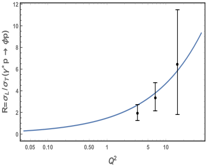
(a)

Figure 10: Ratio $R=\sigma_{L}/\sigma_{T}$ of the total longitudinal to transverse cross sections versus $Q^{2}$, for $\phi$ electro-production as given in (V.59). The blue-solid-curve is for ${\cal N}_{R}=2.6$. The data are from the H1 collaboration Aaron:2009xp

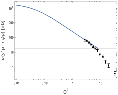
(a)

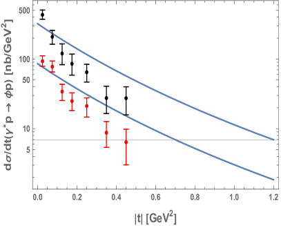
(b)

Figure 11: a: total cross section for $\phi$ electro-production versus $Q^{2}$ for $\sqrt{s}=75\,{\rm GeV}$; b: differential cross section for $\phi$ electro-production versus $|t|$ for $\sqrt{s}=75\,{\rm GeV}$ and $Q^{2}=3.3\,{\rm GeV}^{2}$ (black-data) and $Q^{2}=6.6\,{\rm GeV}^{2}$ (red-data).

The adjusted total cross section for $\phi$ electro-production follows from (III.2.3)

$$\sigma_{tot}(Q^{2})=\mathcal{N}_{Q^{2}}\times\mathcal{\tilde{I}}(\lambda=11.243,Q,\tilde{\kappa}_{\phi}=0.1042~{}\text{GeV})\times\left(1+2.6^{2}\times\left(\frac{1}{2-\frac{1}{\sqrt{11.243}}}\right)^{2}\times\frac{Q^{2}}{1.019^{2}~{}\text{GeV}^{2}}\right)^{1/2}$$

where $\mathcal{\tilde{I}}(\lambda,Q,\tilde{\kappa}_{\phi})$ is given in (III.44) (after replacing $J/\Psi$ by $\phi$), $\mathcal{N}_{R}=2.6$,

$$s=75^{2}~{}\text{GeV}^{2},\lambda=11.243,f_{\phi}=0.233~{}\text{GeV},M_{\phi}=1.019~{}\text{GeV},A^{2}(0)\times\mathbb{N}=3,624.56~{}[nb]\,,$$ (V.61)

and $\tilde{\kappa}_{\phi}=0.1042~{}\text{GeV}$ adjusted to the $\phi$-mass.

In Fig. 11a we show (V.2) versus $Q^{2}$ for $\sqrt{s}=75\,{\rm GeV}$. The data are from the 2010 H1 collaboration at HERA in Aaron:2009xp . In the range $Q^{2}<8\,{\rm GeV}^{2}$, the dependence in $Q^{2}$ supports that from the bulk-to-boundary propagator (III.23) (with the pertinent substitutions) over a decade. The deviation for $Q^{2}\geq 8\,{\rm GeV}^{2}$ signals the on-set of weak coupling as systematically noted in our recent neutrino DIS analysis Mamo:2021cle . In Fig. 11b we show the differential cross section for $\phi$ electro-production versus $|t|$, following from (III.46), after replacing $J/\Psi$ by $\phi$, with

$$s=75^{2}~{}{\rm GeV}^{2},Q=\sqrt{3.3}~{}{\rm GeV},A^{2}(0)\times{\mathbb{N}}^{\prime}=1.98\times 10^{10}~{}[nb/GeV^{2}]\qquad{\rm black-data}$$

$$s=75^{2}~{}{\rm GeV}^{2},Q=\sqrt{6.6}~{}{\rm GeV},A^{2}(0)\times{\mathbb{N}}^{\prime}=2.89\times 10^{10}~{}[nb/GeV^{2}]\qquad{\rm red-data}$$ (V.62)

The data are from the 2010 H1 collaboration at HERA in Aaron:2009xp . The deviations are substantial for moderate values of $t$, which is an indication that Reggeon-like couplings are important in the electro-production of lighter mesons such as $\phi$.

VI Conclusions

The holographic photo-production of charmonium has shown that at treshold the differential cross section probes the tensor gravitational coupling. Away from treshold, the tensor Reggeizes to a Pomeron and the differential cross section probes the Reggeized coupling. We have now extended this analysis to the electro-production of charmonium with a similar observation for the differential cross section.

In the double limit of large $N_{c}$ and strong coupling, only the tensor coupling or A-form factor drives the production of $J/\Psi$ (and also $\Upsilon$) in the treshold region, and its Reggeized form way above treshold. A comparison to the available data at low and intermediate $Q^{2}$ shows that the holographic t-dependence for the total differential cross section for charmonium photo- and electro-production, is consistent with the recent GlueX data and the HERA data over a broad range of $t|$.

In holography, the $Q^{2}$ dependence of the electro-production of charmonium follows from the bulk-to-boundary propagator sourced by the $1^{--}$ current at the boundary such as $\bar{c}\gamma_{\mu}c$. As a result, the longitudinal differential cross section asymptotes $1/Q^{6}$, and the transverse differential cross section asymptotes $1/Q^{8}$, in agreement with the hard scattering rules. At smaller $Q^{2}$, the transverse differential cross section is about constant, while the longitudinal differential cross section vanishes as $Q^{2}$. This limit is fixed by the finite size of charmonium. The holographic results compare well with the HERA data for low and intermediate $Q^{2}$, but depart from the data at larger $Q^{2}$ with the on-set of weak coupling and scaling.

Our results extend miniminally to the $\phi$-channel. The total cross section and the ratio of the longitudinal to transverse cross sections are reasonably well reproduced at low and intermediate $Q^{2}$, but the $|t|$ dependence of the differential cross section is slightly off. This is an indication that Reggeon exchange is likely important in this channe. More data with better accuracy would be welcome.

VII Acknowledgements

K.M. is supported by the U.S. Department of Energy, Office of Science, Office of Nuclear Physics, contract no. DE-AC02-06CH11357, and an LDRD initiative at Argonne National Laboratory under Project No. 2020-0020. I.Z. is supported by the Office of Science, U.S. Department of Energy under Contract No. DE-FG-88ER40388.

VIII kinematics of the $\gamma^{*}p\rightarrow Vp$ process

We start by briefly reviewing the kinematics for the process $\gamma^{*}p\rightarrow Vp$. We first define the Lorentz scalars as $s=W^{2}=(p_{1}+q_{1})^{2}$, and $t=(p_{1}-p_{2})^{2}=(q_{1}-q_{2})^{2}$ where $q_{1,2}$ are the four-vectors of the virtual photon and vector meson, respectively (note that we occasionally use the notation $q\equiv q_{1}$ and $q^{\prime}\equiv q_{2}$), and $p_{1,2}$ are the four vector of the proton. Throughout we will work with mostly negative signature, i.e., $\eta_{\mu\nu}=(+1,-1,-1,-1)$. Note that our convention is different from the mostly positive signature used in most holographic analyses.

We will work in the center-of-mass (CM) frame of the pair composed of the virtual photon $\gamma^{*}$ and the proton. In this frame, one can derive the mathematical relationships between the three-momenta of the virtual photon and vector meson ($\mathbf{q}_{\gamma}$, $\mathbf{q}_{V}$) and Lorentz scalars ($s$, $t$, $q_{1}^{2}=-Q^{2}$, $q_{2}^{2}=M_{V}^{2}$, $p_{1}^{2}=p_{2}^{2}=m_{N}^{2}$) as (see, for example, Eqs.11.2-4 in Srednicki:2007qs )

$$|\mathbf{q}_{\gamma}|=\frac{1}{2\sqrt{s}}\sqrt{s^{2}-2(-Q^{2}+m_{N}^{2})s+(-Q^{2}-m_{N}^{2})^{2}}\,,$$

$$|\mathbf{q}_{V}|=\frac{1}{2\sqrt{s}}\sqrt{s^{2}-2(M_{V}^{2}+m_{N}^{2})s+(M_{V}^{2}-m_{N}^{2})^{2}}\,,$$

and

$$t=-Q^{2}+M_{V}^{2}-2E_{\gamma}E_{V}+2|\mathbf{q}_{\gamma}||\mathbf{q}_{V}|\cos\theta\,,$$

Here $E_{\gamma}=(-Q^{2}+\mathbf{q}_{\gamma}^{2})^{\frac{1}{2}}$ is the energy of the virtual photon, and $E_{V}=(M_{V}^{2}+\mathbf{q}_{V}^{2})^{\frac{1}{2}}$ is the energy of the vector meson. The t-transfer at low $\sqrt{s}$ is bounded by $t_{min}\equiv|t|_{\cos\theta=+1}|$ and $t_{max}\equiv|t|_{\cos\theta=-1}|$ as illustrated in Fig. 12.

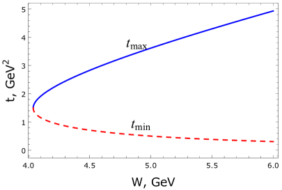
Figure 12: $t_{min}$ and $t_{max}$ vs $W=\sqrt{s}$ for $M_{V}=M_{J/\psi}=3.10~{}GeV$, $m_{N}=0.94~{}GeV$, and $Q=0$. Note that at the threshold energy $W_{tr}=\sqrt{s_{tr}}=m_{N}+M_{V}=4.04~{}GeV$, we have $t_{min}=t_{max}$.

We now note that at threshold and for example $V=J/\Psi$ with $s_{\rm tr}=(m_{N}+M_{V})^{2}=4.04\,{\rm GeV}^{2}$

$$-t_{\rm min}(s=s_{\rm tr})= \frac{m_{N}M^{2}_{V}}{m_{N}+M_{V}}$$

$$= 1.5^{2}\,{\rm GeV}^{2}\ll 4.04^{2}\,{\rm GeV}^{2}=s_{\rm tr}$$

and away from threshold

$$-t_{\rm min}(s\gg s_{\rm tr})\sim\left(\frac{m_{N}M_{V}}{s}\right)^{2}\ll s$$ (VIII.67)

The electro-production kinematics for charmonium and also bottomium, is dominated by the diffractive process all the way to threshold.

IX holographic model

We consider AdS₅ with a background metric $g_{MN}=(\eta_{\mu\nu},-1)/z^{2}$ and $\eta_{\mu\nu}=(1,-1,-1,-1)$. Confinement will be described by a background dilaton $\phi=\tilde{\kappa}_{V}^{2}z^{2}$ for mesons, $\phi=\tilde{\kappa}_{N}^{2}z^{2}$ for protons and $\phi=2\tilde{\kappa}_{N}^{2}z^{2}$ for glueballs in the soft wall model. The glueballs will be described by $h_{\mu\nu}$ and the scalar-dilaton by $\varphi$. The flavor gauge fields will be described by U(1) gauge fields, and the spin-$\frac{1}{2}$ Dirac fermion by $\Psi$.

IX.1 Bulk Dirac fermion and vector meson

The bulk Dirac fermion action in curved AdS₅ with minimal coupling to the U(1) vector meson is  CARLSON

$$S=\int d^{5}x\sqrt{g}\,\big{(}\mathcal{L}_{F}+\mathcal{L}_{V}\big{)}+\int d^{4}x\sqrt{-g^{(4)}}\mathcal{L}_{UV}\,,$$

(IX.68)

with the fermionic, gauge field and boundary actions

$$\mathcal{L}_{F}= \frac{1}{2g_{5}^{2}}e^{-\phi(z)}$$

$$\times\bigg{(}\frac{i}{2}\bar{\Psi}e^{N}_{A}\Gamma^{A}\big{(}\overrightarrow{D}_{N}-\overleftarrow{D}_{N}\big{)}\Psi-(M+V(z))\bar{\Psi}\Psi\bigg{)}\,,$$

$$\mathcal{L}_{V}= -\frac{1}{4g^{2}_{5}}\,e^{-\phi(z)}\,g^{\mu\alpha}g^{\beta\nu}\,F_{\mu\nu}^{V}\,F_{\alpha\beta}^{V}\,,$$

$$\mathcal{L}_{UV}= \frac{1}{2g_{5}^{2}}\left(\bar{\Psi}_{L}\Psi_{R}+\bar{\Psi}_{R}\Psi_{L}\right)_{z=\varepsilon}\,,$$ (IX.69)

We have fixed the potential $V(z)=\tilde{\kappa}_{N}^{2}z^{2}$ for both the soft wall model. We have denoted by $e^{N}_{A}=z\delta^{N}_{A}$ the inverse vielbein, and defined the covariant derivatives

$$\overrightarrow{D}_{N}= \overrightarrow{\partial}_{N}+\frac{1}{8}\omega_{NAB}[\Gamma^{A},\Gamma^{B}]-iV_{N}$$

$$\overleftarrow{D}_{N}= \overleftarrow{\partial}_{N}+\frac{1}{8}\omega_{NAB}[\Gamma^{A},\Gamma^{B}]+iV_{N}$$ (IX.70)

The components of the spin connection are $\omega_{\mu z\nu}=-\omega_{\mu\nu z}=\frac{1}{z}\eta_{\mu\nu}$, the Dirac gamma matrices satisfy anti-commutation relation $\{\Gamma^{A},\Gamma^{B}\}=2\eta^{AB}$, that is, $\Gamma^{A}=(\gamma^{\mu},-i\gamma^{5})$, and $F^{V}_{MN}=\partial_{M}V_{N}-\partial_{N}V_{M}$. The equation of motions for the bulk Dirac fermion and the U(1) gauge field follow by variation

$$\big{[}ie^{N}_{A}\Gamma^{A}D_{N}-\frac{i}{2}(\partial_{N}\phi)\,e^{N}_{A}\Gamma^{A}-(M+\phi(z))\big{]}\Psi=0\,,$$

$$\frac{1}{\sqrt{g}}\partial_{M}\big{(}\sqrt{g}e^{-\phi}F^{MN}\big{)}=0\,.$$

The coupling $g_{5}$ is inherited from the nature of the brane embeddings in bulk: ${1}/{g_{5}^{2}}\equiv{3N_{c}N_{f}}/(12\pi^{2})$ (D7-branes), and ${1}/{g_{5}^{2}}\equiv({3\sqrt{\lambda}}/{2^{5/2}\pi}){N_{c}N_{f}}/({12\pi^{2}})$ (D9-branes). The brane embeddings with $N_{f}=1$ are more appropriate for describing heavy mesons in bulk, as the U(1) field mode decompose in an infinite tower of massive vector mesons on these branes as we discussed above. When ignoring these embedding, the standard assignement is: ${1}/{g_{5}^{2}}\equiv{N_{c}}/(12\pi^{2})$.

We note that in (IX.1), we have excluded a Yukawa-type coupling between the scalar-dilaton $\varphi$ and the bulk Dirac fermion $\Psi$, since neither the fermionic part of the Type IIB supergravity action (see, for example, Eq. A.20 in DHoker:2016ncv ) nor the fermionic part of the DBI action in string theory (see, for example, Eq. 56 in Kirsch:2006he ) support such a coupling.

IX.2 Spectra

For the soft wall model, the vector meson spectrum follows from the equation of motion for $V^{N}$. The results for the heavy meson masses and decay constants are  Grigoryan:2010pj

$$m_{n}^{2}= 4\tilde{\kappa}^{2}_{V}(n^{*}+1)$$

$$g_{5}f_{n}= \sqrt{2}\tilde{\kappa}_{V}\left(\frac{n+1}{n^{*}+1}\right)^{\frac{1}{2}}$$ (IX.72)

with $n^{*}=n+c_{V}^{2}/4\tilde{\kappa}_{V}^{2}$. The additional constant $c_{V}$ is fixed as ${c_{V}^{2}}/{4\tilde{\kappa}_{V}^{2}}={M_{V}^{2}}/{4\tilde{\kappa}_{V}^{2}}-1$ for $n=0$ for the heavy mesons $V=(J/\psi,\Upsilon)$, and $c_{\rho}=0$ for the light mesons. The mass spectrum of the bulk Dirac fermions is given by CARLSON

$$m_{n}^{2}= 4\tilde{\kappa}^{2}_{N}(n+\tau-1)\,,$$ (IX.73)

with the twist factor $\tau=3$. For the specific soft wall applications to follow we will set $\tilde{\kappa}_{N}=\tilde{\kappa}_{\rho}$ for simplicity, unless specified otherwise.

IX.3 Bulk graviton and dilaton

The effective action for the gravitaton ($\eta_{\mu\nu}\rightarrow\eta_{\mu\nu}+h_{\mu\nu}$) and scalar-dilaton fluctuations ($\phi\rightarrow\phi+\varphi$) follows from the Einstein-Hilbert action plus dilaton in the string frame. In de-Donder gauge and to quadratic order, we have

$$S=\int d^{5}x\sqrt{g}\,e^{-2\phi}\big{(}\mathcal{L}_{h+f}+\mathcal{L}_{\varphi}\big{)}\,,$$

(IX.74)

with

$$\mathcal{L}_{h+f}= -\frac{1}{4\tilde{g}_{5}^{2}}\,g^{\mu\nu}\,\eta^{\lambda\rho}\eta^{\sigma\tau}\partial_{\mu}h_{\lambda\sigma}\partial_{\nu}h_{\rho\tau}$$

$$+\frac{1}{8\tilde{g}_{5}^{2}}\,g^{\mu\nu}\eta^{\alpha\beta}\eta^{\gamma\sigma}\,\partial_{\mu}h_{\alpha\beta}\,\partial_{\nu}h_{\gamma\sigma}\,,$$

$$\mathcal{L}_{\varphi}= +\frac{1}{2\tilde{g}_{5}^{2}}\,g^{\mu\nu}\,\partial_{\mu}\varphi\,\partial_{\nu}\varphi\,,$$ (IX.75)

and $\tilde{g}_{5}^{2}=2\kappa^{2}=16\pi G_{N}={8\pi^{2}}/{N_{c}^{2}}$. The graviton in bulk is dual to a glueball on the boundary. We follow Kanitscheider:2008kd , and split $h_{\mu\nu}$ into a traceless part $h$ (tensor $2^{++}$ glueball) and and trace-full part $f$ (scalar $0^{++}$ glueball)

$$h_{\mu\nu}(k,z)=\bigg{[}\epsilon_{\mu\nu}^{TT}h(k,z)+k_{\mu}k_{\nu}H(k,z)\bigg{]}+\bigg{[}k_{\mu}A^{\perp}_{\nu}(k,z)+k_{\nu}A^{\perp}_{\mu}(k,z)\bigg{]}+\bigg{[}\frac{1}{3}\eta_{\mu\nu}f(k,z)\bigg{]}$$ (IX.76)

with $k^{\mu}\epsilon_{\mu\nu}^{TT}=\eta^{\mu\nu}\epsilon_{\mu\nu}^{TT}=0$. A further gauge fixing $A_{\mu}^{\perp}=0$, allows to decouple the tensor glueball $h$. In contrast, the equations for $f$, $H$, and $\varphi$ (denoted as $k$ in Kanitscheider:2008kd ) are coupled (see Eqs.7.16-20 in Kanitscheider:2008kd ). Diagonalizing the equations, one can show that $f$ satisfies the same equation of motion as $h$ Kanitscheider:2008kd . Also note that $f_{0}=f(z=0)$ couples to $T^{\mu}_{\mu}$ of the gauge theory, while $H_{0}=H(z=0)$ couples to $k^{\mu}k^{\nu}T_{\mu\nu}\equiv 0$ (see Eq.7.6 of Kanitscheider:2008kd ).

The ensuing spectra for the tensor $2^{++}$ and scalar $0^{++}$ glueballs are degenerate HILMAR

$$m_{T,S}^{2}(n)=8\tilde{\kappa}^{2}_{N}\bigg{(}n+2\bigg{)}\qquad(T:\tilde{g}_{5}f_{n},\,\,\,S:\sqrt{2}\tilde{g}_{5}f_{n})\rightarrow 2\tilde{\kappa}_{N}$$ (IX.77)

They differ from their vector meson counterparts in (IX.2) by the replacements $\tilde{\kappa}_{V}\rightarrow\sqrt{2}\tilde{\kappa}_{N}$ and $g_{5}\rightarrow\tilde{g}_{5}$ due to the difference in the bulk actions. The spectrum of the scalar-dilaton fluctuations and coupling are similar to the tensor glueball.

The bulk graviton couplings are

$$h\overline{\Psi}\Psi:\quad -\frac{\sqrt{2\kappa^{2}}}{2}\int d^{5}x\,\sqrt{g}\,h_{\mu\nu}T_{F}^{\mu\nu}$$

$$hAA:\quad -\frac{\sqrt{2\kappa^{2}}}{2}\int d^{5}x\,\sqrt{g}\,h_{\mu\nu}T_{V}^{\mu\nu}$$

with the energy-momentum tensors

$$T_{F}^{\mu\nu} = e^{-\phi}\frac{i}{2}\,z\,\overline{\Psi}\gamma^{\mu}\overset{\leftrightarrow}{\partial^{\nu}}\Psi-\eta^{\mu\nu}\mathcal{L}_{F}\,,$$

$$T_{V}^{\mu\nu} = -e^{-\phi}\Big{(}z^{4}\eta^{\rho\sigma}\eta^{\mu\beta}\eta^{\nu\gamma}\,F^{V}_{\beta\rho}F^{V}_{\gamma\sigma}$$

$$-z^{4}\,\eta^{\mu\beta}\eta^{\nu\gamma}\,F^{V}_{\beta z}F^{V}_{\gamma z}\Big{)}-\eta^{\mu\nu}\mathcal{L}_{V}\,.$$

There is no contribution from the UV-boundary term in (IX.68) since it vanishes for the normalizable modes of the fermion. The scalar-dilaton couplings are

$$\varphi\bar{\Psi}\Psi:\quad \sqrt{2\kappa^{2}}\int d^{5}x\,\sqrt{g}\,\frac{e^{-\phi}}{2}\,\left(\frac{z}{2}\,\partial_{z}\varphi\right)\,\overline{\Psi}\gamma^{5}\Psi+\sqrt{2\kappa^{2}}\int d^{5}x\,\sqrt{g}\,\frac{e^{-\phi}}{2}\,\left(\frac{iz}{2}\,\partial_{\mu}\varphi\right)\,\overline{\Psi}\gamma^{\mu}\Psi$$

$$\varphi AA:\quad \sqrt{2\kappa^{2}}\int d^{5}x\,\sqrt{g}\,e^{-\phi}\,(-\varphi)\,\left(-\frac{1}{4}\,g^{\mu\alpha}g^{\beta\nu}\,F_{\mu\nu}^{V}\,F_{\alpha\beta}^{V}\right)$$ (IX.80)

To make the power counting manifest in the Witten diagrams, we canonically rescale the fields as

$$\Psi\rightarrow g_{5}\Psi\qquad V_{N}\rightarrow g_{5}V_{N}\qquad\varphi\rightarrow\sqrt{2\kappa^{2}}\,\varphi\qquad h_{\mu\nu}\rightarrow\sqrt{2\kappa^{2}}\,h_{\mu\nu}$$ (IX.81)

which makes the couplings and power counting manifest.Note that after this rescaling, the meson decay constants in (IX.2) and the glueball decay constants in (IX.77) redefine through $g_{5}f_{n}\rightarrow f_{n}$. This is understood in most of our analysis.

X wavefunctions in holographic QCD

X.1 Dirac fermion/proton

The normalized wavefunctions for the bulk Dirac fermion are CARLSON

$$\Psi(p,z) = \psi_{R}(z)\Psi^{0}_{R}(p)+\psi_{L}(z)\Psi^{0}_{L}(p)\,,$$

$$\bar{\Psi}(p,z) = \psi_{R}(z)\bar{\Psi}^{0}_{R}(p)+\psi_{L}(z)\bar{\Psi}^{0}_{L}(p)\,,$$

with for the soft-wall ($\tau=3$)

$$\psi_{R}(z)=\frac{\tilde{n}_{R}}{\tilde{\kappa}_{N}^{\tau-2}}z^{\frac{5}{2}}\xi^{\frac{\tau-2}{2}}L_{0}^{(\tau-2)}(\xi)\,,$$

$$\psi_{L}(z)=\frac{\tilde{n}_{L}}{\tilde{\kappa}_{N}^{\tau-1}}z^{\frac{5}{2}}\xi^{\frac{\tau-1}{2}}L_{0}^{(\tau-1)}(\xi)\,,$$

$L_{n}^{(\alpha)}(\xi)$, $\tilde{n}_{R}=\tilde{n}_{L}\tilde{\kappa}_{N}^{-1}\sqrt{\tau-1}$ are the generalized Laguerre polynomials, and $\tilde{n}_{L}=\tilde{\kappa}_{N}^{\tau}\sqrt{{2}/{\Gamma(\tau)}}$. The bulk wave functions are normalized

$$\int_{0}^{\infty}dz\,\sqrt{g}\,e^{-\phi}\,e^{\mu}_{a}\,\psi_{R/L}^{2}(z)=\delta^{\mu}_{a}\,,$$

with $\phi=\tilde{\kappa}_{N}^{2}z^{2}$, and the inverse vielbein $e^{\mu}_{a}=\sqrt{{\left|g^{\mu\mu}\right|}}\delta^{\mu}_{a}$ (no summation intended in $\mu$). $\Psi^{0}_{R/L}(p)=P_{\pm}u(p)$, $\bar{\Psi}^{0}_{R/L}(p)=\bar{u}(p)P_{\mp}$, and $P_{\pm}=(1/2)(1\pm\gamma^{5})$. The boundary spinors are normalized as

$$\bar{u}(p)u(p)=2m_{N}\,,$$

$$2m_{N}\times\bar{u}(p^{\prime})\gamma^{\mu}u(p)=\bar{u}(p^{\prime})(p^{\prime}+p)^{\mu}u(p)\,.$$

X.2 Photon/spin-1 mesons

The vector wavefunctions are given by Grigoryan:2007my

$$\phi_{n}(z)=c_{n}\tilde{\kappa}_{V}^{2}z^{2}L_{n}^{1}(\tilde{\kappa}_{V}^{2}z^{2})\equiv J_{A}(m_{n},z)\,,$$ (X.86)

with $c_{n}=\sqrt{{2}/{n+1}}$ which is determined from the normalization condition (for the soft-wall model with background dilaton $\phi=\tilde{\kappa}_{V}^{2}z^{2}$)

$$\int dz\,\sqrt{g}e^{-\phi}\,(g^{xx})^{2}\,\phi_{n}(z)\phi_{m}(z)=\delta_{nm}\,.$$

Therefore, we have

$$F_{n}=\frac{1}{g_{5}}\bigg{(}-e^{-\phi}\frac{1}{z^{\prime}}\partial_{z^{\prime}}\phi_{n}(z^{\prime})\bigg{)}_{z^{\prime}=\epsilon}=-\frac{2}{g_{5}}c_{n}(n+1)\tilde{\kappa}_{V}^{2}\,,$$

with $\phi_{n}(z\rightarrow 0)\approx c_{n}\tilde{\kappa}_{V}^{2}z^{2}(n+1)$. If we define the decay constant as $f_{n}=-{F_{n}}/{m_{n}}$, we have

$$\phi_{n}(z)=\frac{f_{n}}{m_{n}}\times 2g_{5}\tilde{\kappa}_{V}^{2}z^{2}L_{n}^{1}(\tilde{\kappa}_{V}^{2}z^{2})\,,$$ (X.89)

as required by vector meson dominance (VMD).

The bulk-to-bulk propagator is

$$G(z\rightarrow 0,z^{\prime}) \approx\frac{\phi_{n}(z\rightarrow 0)}{-g_{5}F_{n}}\sum_{n}\frac{-g_{5}F_{n}\phi_{n}(z^{\prime})}{q^{2}-m_{n}^{2}}=\frac{z^{2}}{2}\sum_{n}\frac{-g_{5}F_{n}\phi_{n}(z^{\prime})}{q^{2}-m_{n}^{2}}=\frac{z^{2}}{2}V(q,z^{\prime}).$$

For space-like momenta ($q^{2}=-Q^{2}$), we have the bulk-to-bulk propagator near the boundary

$$G(z\rightarrow 0,z^{\prime})\approx\frac{z^{2}}{2}\sum_{n}\frac{g_{5}F_{n}\phi_{n}(z^{\prime})}{Q^{2}+m_{n}^{2}}=\frac{z^{2}}{2}\mathcal{V}(Q,z^{\prime})\,,$$

(X.91)

with Grigoryan:2007my

$$\mathcal{V}(Q,z)=\kappa_{V}^{2}z^{2}\int_{0}^{1}\frac{dx}{(1-x)^{2}}x^{a}{\rm exp}\Big{[}-\frac{x}{1-x}\kappa_{V}^{2}z^{2}\Big{]}\,,$$

(X.92)

and the normalization ${\cal V}(0,z)={\cal V}(Q,0)=1$.

X.3 Tansverse-traceless graviton/spin-2 glueballs

Similar relationships hold for the soft-wall model where the normalized wave function for spin-2 glueballs is given by BallonBayona:2007qr (note that the discussion in BallonBayona:2007qr is for general massive bulk scalar fluctuation but can be used for spin-2 glueball which has an effective bulk action similar to massless bulk scalar fluctuation)

$$\psi_{n}(z)=c_{n}\,z^{4}L_{n}^{\Delta(j)-2}(2\xi)\,,$$

with

$$c_{n}=\Bigg{(}\frac{2^{4}\tilde{\kappa}_{N}^{6}\Gamma(n+1)}{\Gamma(n+3)}\Bigg{)}^{\frac{1}{2}}\,,$$ (X.94)

which is determined from the normalization condition (for soft-wall model with background dilaton $\phi=\tilde{\kappa}_{N}^{2}z^{2}$)

$$\int dz\,\sqrt{g}e^{-\phi}\,{\left|g^{xx}\right|}\,\psi_{n}(z)\psi_{m}(z)=\delta_{nm}\,.$$

Therefore we have

$$F_{n}=\frac{1}{\sqrt{2}\kappa}\bigg{(}-\frac{1}{z^{\prime 3}}\partial_{z^{\prime}}\psi_{n}(z^{\prime})\bigg{)}_{z^{\prime}=\epsilon}=-\frac{4}{\sqrt{2}\kappa}c_{n}L_{n}^{2}(0)\,,$$

with $\psi_{n}(z\rightarrow 0)\approx c_{n}\,z^{4}L_{n}^{2}(0)$. For space-like momenta ($q^{2}=-Q^{2}$), we have the bulk-to-bulk propagator near the boundary

$$G(z\rightarrow 0,z^{\prime})\approx\frac{z^{4}}{4}\sum_{n}\frac{\sqrt{2}\kappa F_{n}\phi_{n}(z^{\prime})}{K^{2}+m_{n}^{2}}=\frac{z^{4}}{4}\mathcal{H}(K,z^{\prime}),$$

(X.97)

where, for the soft-wall model, CARLSON ; Abidin:2008ku ; BallonBayona:2007qr

$$\mathcal{H}(K,z) =4z^{4}\Gamma(a_{K}+2)U\Big{(}a_{K}+2,3;2\xi\Big{)}=\Gamma(a_{K}+2)U\Big{(}a_{K},-1;2\xi\Big{)}$$ (X.98)

$$=\frac{\Gamma(a_{K}+2)}{\Gamma(a_{K})}\int_{0}^{1}dx\,x^{a_{K}-1}(1-x){\rm exp}\Big{(}-\frac{x}{1-x}(2\xi)\Big{)}\,,$$

with $a_{K}={a}/{2}={K^{2}}/{8\tilde{\kappa}_{N}^{2}}$, and we have used the transformation $U(m,n;y)=y^{1-n}U(1+m-n,2-n,y)$. (X.98) satisfies the normalization condition ${\cal H}(0,z)={\cal H}(K,0)=1$.

XI Details of the holographic differential cross section: near threshold

The holographic differential cross section for untraced in and out polarizations read

$$\frac{d\sigma(s,t,Q,M_{J/\Psi},\epsilon_{T},\epsilon^{\prime}_{T})}{dt}=\frac{e^{2}}{16\pi(s-(-Q^{2}+m_{N}^{2}))^{2}}\,\frac{1}{2}\sum_{{\rm spin}}\Bigg{|}{\cal A}^{TT}_{\gamma^{*}p\rightarrow J/\Psi p}(s,t,Q,M_{J/\Psi},\epsilon_{T},\epsilon^{\prime}_{T})\Bigg{|}^{2}\,,$$

$$\frac{d\sigma(s,t,Q,M_{J/\Psi},\epsilon_{L},\epsilon^{\prime}_{L})}{dt}=\frac{e^{2}}{16\pi(s-(-Q^{2}+m_{N}^{2}))^{2}}\,\frac{1}{2}\sum_{{\rm spin}}\Bigg{|}{\cal A}^{LL}_{\gamma^{*}p\rightarrow J/\Psi p}(s,t,Q,M_{J/\Psi},\epsilon_{L},\epsilon^{\prime}_{L})\Bigg{|}^{2}\,,$$ (XI.99)

where the transverse and longitudinal amplitudes are respectively

$${\cal A}^{TT}_{\gamma^{*}p\rightarrow J/\Psi p}(s,t,Q,M_{J/\Psi},\epsilon_{T},\epsilon^{\prime}_{T})=$$

$$\frac{1}{g_{5}}\times\Big{(}\mathcal{I}(Q,M_{J/\Psi})\times B_{1}^{TT}-\mathcal{J}(Q,M_{J/\Psi})\times B_{0}^{TT}Q^{2}\Big{)}\times 2\kappa^{2}\times A(K)\times\frac{1}{m_{N}}\,\bar{u}(p_{2})u(p_{1})\,,$$

$${\cal A}^{LL}_{\gamma^{*}p\rightarrow J/\Psi p}(s,t,Q,M_{J/\Psi},\epsilon_{L},\epsilon^{\prime}_{L})=$$

$$\frac{1}{g_{5}}\times\Big{(}\mathcal{I}(Q,M_{J/\Psi})\times B_{1}^{LL}-\mathcal{J}(Q,M_{J/\Psi})\times B_{0}^{LL}Q^{2}\Big{)}\times 2\kappa^{2}\times A(K)\times\frac{1}{m_{N}}\,\bar{u}(p_{2})u(p_{1})\,,$$

with

$$B_{1}^{TT}(s,t,Q,M_{J/\Psi}) = p_{\alpha}p_{\beta}B_{1}^{\alpha\beta}(\epsilon_{T},\epsilon^{\prime}_{T})=\epsilon_{T}\cdot\epsilon^{\prime}_{T}\,q\cdot p\,q^{\prime}\cdot p+q\cdot q^{\prime}\,\epsilon_{T}\cdot p\,\,\epsilon^{\prime}_{T}\cdot p-q\cdot\epsilon^{\prime}_{T}\,p\cdot\epsilon_{T}\,p\cdot q^{\prime}-q^{\prime}\cdot\epsilon_{T}\,p\cdot\epsilon^{\prime}_{T}\,p\cdot q\,,$$

$$B_{1}^{LL}(s,t,Q,M_{J/\Psi}) = p_{\alpha}p_{\beta}B_{1}^{\alpha\beta}(\epsilon_{L},\epsilon^{\prime}_{L})=\epsilon_{L}\cdot\epsilon^{\prime}_{L}\,q\cdot p\,q^{\prime}\cdot p+q\cdot q^{\prime}\,\epsilon_{L}\cdot p\,\,\epsilon^{\prime}_{L}\cdot p-q\cdot\epsilon^{\prime}_{L}\,p\cdot\epsilon_{L}\,p\cdot q^{\prime}-q^{\prime}\cdot\epsilon_{L}\,p\cdot\epsilon^{\prime}_{L}\,p\cdot q\,,$$

$$B_{0}^{TT}(s,t,Q,M_{J/\Psi}) = p_{\alpha}p_{\beta}B_{0}^{\alpha\beta}(\epsilon_{T},\epsilon^{\prime}_{T})=\epsilon_{T}\cdot p\,\,\epsilon^{\prime}_{T}\cdot p\,,$$

$$B_{0}^{LL}(s,t,Q,M_{J/\Psi}) = p_{\alpha}p_{\beta}B_{0}^{\alpha\beta}(\epsilon_{L},\epsilon^{\prime}_{L})=\epsilon_{L}\cdot p\,\,\epsilon^{\prime}_{L}\cdot p\,,$$ (XI.101)

where we will make use of the orthogonality conditions

$$\epsilon_{L}\cdot q=\epsilon_{L}^{0}q_{0}-|\vec{\epsilon}_{L}|q_{z}\cos\theta^{\prime}=0$$ (XI.102)

and

$$\epsilon_{L}^{\prime}\cdot q^{\prime}=\epsilon_{L}^{\prime 0}q^{\prime}_{0}-|\vec{\epsilon}_{L}^{\prime}||\mathbf{q}_{V}|\cos\theta^{\prime\prime}=0$$ (XI.103)

in order to evaluate

$$\epsilon_{L}\cdot q^{\prime}=\epsilon_{L}^{0}q^{\prime}_{0}-|\vec{\epsilon}_{L}||\mathbf{q}_{V}|\cos(\theta^{\prime}+\theta)\,,$$ (XI.104)

and

$$\epsilon_{L}^{\prime}\cdot q=\epsilon_{L}^{\prime 0}q_{0}-|\vec{\epsilon}_{L}^{\prime}|q_{z}\cos(\theta^{\prime\prime}+\theta)\,.$$ (XI.105)

Also note that we will use $\epsilon_{L}^{2}=-1$ and $\epsilon{{}^{\prime}2}_{L}=-1$ in order to find

$$|\vec{\epsilon}_{L}|=\sqrt{\frac{Q^{2}+q_{z}^{2}}{Q^{2}}}\,,\quad\quad\quad|\vec{\epsilon}_{L}^{\prime}|=\sqrt{\frac{M_{V}^{2}+|\mathbf{q}_{V}|^{2}}{M_{V}^{2}}}\,.$$ (XI.106)

For the transverse part we use

$$\epsilon_{T}\cdot\epsilon_{T}^{\prime}=-|\vec{\epsilon}_{T}||\vec{\epsilon}^{\prime}_{T}|\cos\theta=-\cos\theta\,,$$ (XI.107)

$$\epsilon_{T}\cdot q^{\prime}=-|\vec{\epsilon}_{T}||\mathbf{q}_{V}|\cos\left(\frac{\pi}{2}+\theta\right)=-|\mathbf{q}_{V}|\sin\theta\,,$$ (XI.108)

and

$$\epsilon_{T}^{\prime}\cdot q=-|\vec{\epsilon}_{T}^{\prime}|q_{z}\cos\left(\frac{\pi}{2}-\theta\right)=-q_{z}\sin(\theta)\,.$$ (XI.109)

In addition, we have defined

$$\mathcal{I}(Q,M_{J/\Psi})= \Big{(}\frac{\tilde{\kappa}_{J/\Psi}}{Q}\Big{)}^{4}\times\frac{1}{2}\int_{0}^{\infty}d\xi\,e^{-\xi^{2}\frac{\tilde{\kappa}_{J/\Psi}^{2}}{Q^{2}}}\,\xi^{-1}\times\mathcal{V}_{\gamma^{*}}(\xi)\mathcal{V}_{J/\Psi}(\xi M_{J/\Psi}/Q)\times\frac{\xi^{4}}{4}$$

$$= \frac{f_{J/\Psi}}{M_{J/\Psi}}\times g_{5}\times\Bigg{(}\frac{3}{\frac{1}{32}\frac{Q^{6}}{\tilde{\kappa}_{J/\Psi}^{6}}+\frac{3}{4}\frac{Q^{4}}{\tilde{\kappa}_{J/\Psi}^{4}}+\frac{11}{2}\frac{Q^{2}}{\tilde{\kappa}_{J/\Psi}^{2}}+12}\Bigg{)}$$

$$= \frac{1}{2}\frac{f_{J/\Psi}}{M_{J/\Psi}}\times g_{5}\times\left(\frac{3}{\left(\frac{Q^{2}}{4\tilde{\kappa}_{J/\Psi}^{2}}+3\right)\left(\frac{Q^{2}}{4\tilde{\kappa}_{J/\Psi}^{2}}+2\right)\left(\frac{Q^{2}}{4\tilde{\kappa}_{J/\Psi}^{2}}+1\right)}\right)\,,$$

$$\mathcal{J}(Q,M_{J/\Psi})= \Big{(}\frac{\tilde{\kappa}_{J/\Psi}}{Q}\Big{)}^{4}\times\frac{1}{2}\int_{0}^{\infty}d\xi\,e^{-\xi^{2}\frac{\tilde{\kappa}_{J/\Psi}^{2}}{Q^{2}}}\,\xi^{-1}\times\partial_{\xi}\mathcal{V}_{\gamma^{*}}(\xi)\times\partial_{\xi}\mathcal{V}_{J/\Psi}(\xi M_{J/\Psi}/Q)\times\frac{\xi^{4}}{4}$$

$$= -\frac{f_{J/\Psi}}{M_{J/\Psi}}\times g_{5}\times\Bigg{(}\frac{1}{\frac{1}{32}\frac{Q^{6}}{\tilde{\kappa}_{J/\Psi}^{6}}+\frac{3}{4}\frac{Q^{4}}{\tilde{\kappa}_{J/\Psi}^{4}}+\frac{11}{2}\frac{Q^{2}}{\tilde{\kappa}_{J/\Psi}^{6}}+12}\Bigg{)}$$

$$= -\frac{1}{3}\times\mathcal{I}(Q,M_{J/\Psi})\,,$$ (XI.110)

with $\xi\equiv Qz$.

Following the general invariant decomposition

$$\left<p_{2}|T^{\mu\nu}(0)|p_{1}\right>=\overline{u}(p_{2})\left(A(k)\gamma^{(\mu}p^{\nu)}+B(k)\frac{ip^{(\mu}\sigma^{\nu)\alpha}k_{\alpha}}{2m_{N}}+C(k)\frac{k^{\mu}k^{\nu}-\eta^{\mu\nu}k^{2}}{m_{N}}\right)u(p_{1})\,,$$ (XI.111)

the tensor gravitational form factor is

$$A=\frac{1}{2}\int dz\sqrt{g}\,e^{-\phi}z\,\big{(}\psi_{R}^{2}(z)+\psi_{L}^{2}(z)\big{)}\,\mathcal{H}(K,z)$$ (XI.112)

and $B(0)=0$, in the present holographic construction. The trace is normalized $\left<p|T^{\mu}_{\mu}|p\right>=2A(0)m_{N}^{2}$. Specifically, for the soft wall model, we have

$$A(K)=A(0)\bigg{(}(1-2a_{K})(1+a_{K}^{2})+a_{K}(1+a_{K})(1+2a_{K}^{2})\bigg{(}H\bigg{(}\frac{1+a_{K}}{2}\bigg{)}-H\bigg{(}\frac{a_{K}}{2}\bigg{)}\bigg{)}\bigg{)}$$ (XI.113)

with $a_{K}={K^{2}}/{8\tilde{\kappa}_{N}^{2}}$. Here $H(x)$ is the harmonic number $H(x)=\psi(1+x)+\gamma$. The gravitational form factor $B(K)$ is found to be null, and the gravitational form factor $C(K)$ is fixed by both the tensor and scalar glueball contributions. It will not be needed here. Since the boundary value ${\cal H}(K,0)={\cal H}(0,z)$ is arbitrary (1-point function), it follows that $A(0)$ is not fixed in holography.

Finally, evaluating the spin sum over the initial and final bulk Dirac fermions, we find

$$\frac{d\sigma(s,t,Q,M_{J/\Psi},\epsilon_{T},\epsilon^{\prime}_{T})}{dt} = \frac{e^{2}\times\frac{(2\kappa^{2})^{2}}{g_{5}^{2}}}{16\pi(s-(-Q^{2}+m_{N}^{2}))^{2}}\,\frac{1}{2}\times\left(\frac{s}{\tilde{\kappa}_{N}^{2}}\right)^{4}\times\mathcal{I}^{2}(Q,M_{J/\Psi})\times\frac{\tilde{\kappa}_{N}^{8}}{\tilde{\kappa}_{J/\Psi}^{8}}$$

$$\times\frac{1}{s^{4}}\tilde{F}^{TT}(s,t,Q,M_{J/\Psi},m_{N})\times(2K^{2}+8m_{N}^{2})\times\frac{1}{m_{N}^{2}}\times A^{2}(t)\,,$$

$$\frac{d\sigma(s,t,Q,M_{J/\Psi},\epsilon_{L},\epsilon^{\prime}_{L})}{dt} = \frac{e^{2}\times\frac{(2\kappa^{2})^{2}}{g_{5}^{2}}}{16\pi(s-(-Q^{2}+m_{N}^{2}))^{2}}\,\frac{1}{2}\times\left(\frac{s}{\tilde{\kappa}_{N}^{2}}\right)^{4}\times\mathcal{I}^{2}(Q,M_{J/\Psi})\times\frac{\tilde{\kappa}_{N}^{8}}{\tilde{\kappa}_{J/\Psi}^{8}}$$ (XI.114)

$$\times\frac{1}{s^{4}}\tilde{F}^{LL}(s,t,Q,M_{J/\Psi},m_{N})\times(2K^{2}+8m_{N}^{2})\times\frac{1}{m_{N}^{2}}\times A^{2}(t)$$

where we have used the spin sum

$$\sum_{s,s^{\prime}}\bar{u}_{s^{\prime}}(p_{2})u_{s}(p_{1})\bar{u}_{s}(p_{1})u_{s^{\prime}}(p_{2}) = {\rm Tr}\Big{(}\sum_{s.s^{\prime}}u_{s^{\prime}}(p_{2})\bar{u}_{s^{\prime}}(p_{2})u_{s}(p_{1})\bar{u}_{s}(p_{1})\Big{)}$$ (XI.115)

$$= \frac{1}{4}{\rm Tr}\Big{(}\big{(}\gamma_{\mu}p_{2}^{\mu}+m_{N}\big{)}\big{(}\gamma_{\mu}p_{1}^{\mu}+m_{N}\big{)}\Big{)}=2K^{2}+8m_{N}^{2}\,,$$

and defined the kinematic factors coming from the polarization tensors as

$$\tilde{F}^{TT}(s,t,Q,M_{J/\Psi},m_{N}) = \Big{[}B_{1}^{TT}(s,t,Q,M_{J/\Psi})\Big{]}^{2}+\frac{1}{9}\times\Big{[}B_{0}^{TT}(s,Q,M_{J/\Psi})Q^{2}\Big{]}^{2}$$

$$- 2\times\frac{1}{3}\times B_{1}^{TT}(s,t,Q,M_{J/\Psi})\times B_{0}^{TT}(s,t,Q,M_{J/\Psi})Q^{2}\,,$$

$$\tilde{F}^{LL}(s,t,Q,M_{J/\Psi},m_{N}) = \Big{[}B_{1}^{LL}(s,t,Q,M_{J/\Psi})\Big{]}^{2}+\frac{1}{9}\times\Big{[}B_{0}^{LL}(s,t,Q,M_{J/\Psi})Q^{2}\Big{]}^{2}$$ (XI.116)

$$- 2\times\frac{1}{3}\times B_{1}^{LL}(s,t,Q,M_{J/\Psi})\times B_{0}^{LL}(s,t,Q,M_{J/\Psi})Q^{2}\,.$$

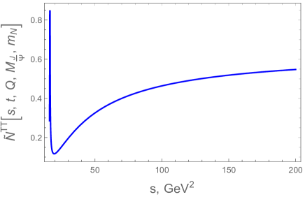
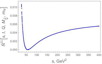
Figure 13: The rescaled transverse normalization coefficient in (XI) (top), and rescaled longitudinal normalization coefficient in (XI) (bottom), for $t=-1~{}{\rm GeV}^{2}$, $Q=1~{}{\rm GeV}$, $M_{J/\Psi}=3.10~{}{\rm GeV}$ and $m_{N}=0.94~{}{\rm GeV}$.

We can further rewrite the differential cross sections more compactly as

$$\frac{d\sigma(s,t,Q,M_{J/\Psi},\epsilon_{T},\epsilon^{\prime}_{T})}{dt} = \mathcal{I}^{2}(Q,M_{J/\Psi})\times\left(\frac{s}{\tilde{\kappa}_{N}^{2}}\right)^{2}\times\mathcal{N}^{TT}(s,t,Q,M_{J/\Psi},m_{N})\times\left(-\frac{t}{4m_{N}^{2}}+1\right)\times\tilde{A}^{2}(t)\,,$$

$$\frac{d\sigma(s,t,Q,M_{J/\Psi},\epsilon_{L},\epsilon^{\prime}_{L})}{dt} = \mathcal{I}^{2}(Q,M_{J/\Psi})\times\left(\frac{s}{\tilde{\kappa}_{N}^{2}}\right)^{2}\times\frac{1}{9}\times\frac{Q^{2}}{M_{J/\Psi}^{2}}\times\mathcal{N}^{LL}(s,t,Q,M_{J/\Psi},m_{N})\times\left(-\frac{t}{4m_{N}^{2}}+1\right)\times\tilde{A}^{2}(t)\,,$$

where we have defined the normalization coefficients as

$$\mathcal{N}^{TT}(s,t,Q,M_{J/\Psi},m_{N}) = \frac{e^{2}\times\frac{(2\kappa^{2})^{2}}{g_{5}^{2}}}{16\pi(1-(-\frac{Q^{2}}{s}+\frac{m_{N}^{2}}{s}))^{2}}\,\frac{1}{2}\times\frac{\tilde{\kappa}_{N}^{4}}{\tilde{\kappa}_{J/\Psi}^{8}}\times A^{2}(0)$$

$$\times \frac{1}{s^{4}}\tilde{F}^{TT}(s,t,Q,M_{J/\Psi},m_{N})\times 8\,,$$

$$\mathcal{N}^{LL}(s,t,Q,M_{J/\Psi},m_{N}) = \frac{e^{2}\times\frac{(2\kappa^{2})^{2}}{g_{5}^{2}}}{16\pi(1-(-\frac{Q^{2}}{s}+\frac{m_{N}^{2}}{s}))^{2}}\times\frac{1}{2}\times\frac{\tilde{\kappa}_{N}^{4}}{\tilde{\kappa}_{J/\Psi}^{8}}\times A^{2}(0)\,$$

$$\times 9\times\frac{M_{J/\Psi}^{2}}{Q^{2}}\times\frac{1}{s^{4}}\tilde{F}^{LL}(s,t,Q,M_{J/\Psi},m_{N})\times 8\,$$

and we have normalized the gravitational form factor $A(t)$ to be unity at $t=0$ as

$$\tilde{A}(t)\equiv\frac{A(t)}{A(0)}\,.$$ (XI.119)

The $TT$ and $LL$ kinematical functions $\tilde{F}$ in (XI) are given in (XI). In Figs. 13 we show the behavior of the rescaled normalizations (XI) over a broad range of $s$. The rescaling is through ${\cal N}\rightarrow\tilde{\cal N}={\cal N}/f$ with all holographic couplings lumped in

$$f\equiv f_{TT,LL}=\Bigg{[}{e^{2}\frac{(2\kappa^{2})^{2}}{32\pi g_{5}^{2}}\frac{\tilde{\kappa}_{N}^{4}}{\tilde{\kappa}_{J/\Psi}^{8}}}\times\frac{1}{\left(-\frac{t}{4m_{N}^{2}}+1\right)}~{},~{}{e^{2}\frac{(2\kappa^{2})^{2}}{32\pi g_{5}^{2}}\frac{\tilde{\kappa}_{N}^{4}}{\tilde{\kappa}_{J/\Psi}^{8}}}\times 9\times\frac{M_{J/\Psi}^{2}}{Q^{2}}\times\frac{1}{\left(-\frac{t}{4m_{N}^{2}}+1\right)}\Bigg{]}\,.$$

For heavy vector mesons, like $J/\Psi$, we can assume $s\sim s_{threshold}\gg m_{N}^{2}$, and on top of that if we restrict ourselves to $s\sim s_{threshold}\gg Q^{2},M_{V}^{2},|t|$, we have $\epsilon_{L}^{\mu}(s\rightarrow\infty)=\frac{q^{\mu}}{Q}$, $\epsilon_{L}^{\prime\mu}(s\rightarrow\infty)=\frac{q^{\prime\mu}}{M_{V}}$, and $\theta(s\rightarrow\infty)=0$ hence $\epsilon_{T}\cdot\epsilon^{\prime}_{T}(s\rightarrow\infty)=-1$, $\epsilon_{T}\cdot A(s\rightarrow\infty)=\epsilon^{\prime}_{T}\cdot A(s\rightarrow\infty)=0$ for $A=q,q^{\prime},p,p_{1},p_{2}$. Therefore, for heavy mesons, we have

$$\tilde{F}(s)= \tilde{F}^{TT}(s\rightarrow\infty,t,Q,M_{J/\Psi},m_{N})$$

$$= 9\times\frac{M_{J/\Psi}^{2}}{Q^{2}}\times\tilde{F}^{LL}(s\rightarrow\infty,t,Q,M_{J/\Psi},m_{N})$$

$$= Q^{2}M_{J/\Psi}^{2}\times\Big{[}B_{0}^{LL}(s\rightarrow\infty,t,Q,M_{J/\Psi})\Big{]}^{2}$$

$$= \Big{[}B_{1}^{TT}(s\rightarrow\infty,t,Q,M_{J/\Psi})\Big{]}^{2}$$

$$= \lim_{s\to\infty}(q\cdot p\,q^{\prime}\cdot p)^{2}=\lim_{s\to\infty}(2q_{z}^{2})^{4}=\frac{1}{16}\times s^{4}\,,$$ (XI.121)

which simplifies the normalization coefficients to

$$\mathcal{N}^{TT}(s,t,Q,M_{J/\Psi},m_{N}) \approx \frac{e^{2}\times\frac{(2\kappa^{2})^{2}}{g_{5}^{2}}}{16\pi}\,\frac{1}{2}\times\frac{\tilde{\kappa}_{N}^{4}}{\tilde{\kappa}_{J/\Psi}^{8}}\times A^{2}(0)\times\frac{1}{s^{4}}\tilde{F}(s)\times 8=constant\,,$$

$$\mathcal{N}^{LL}(s,t,Q,M_{J/\Psi},m_{N}) \approx \mathcal{N}^{TT}(s,t,Q,M_{J/\Psi},m_{N})\,,$$

where $\frac{1}{s^{4}}\tilde{F}(s)=\frac{1}{16}$.

XII Details of the holographic differential cross section: high energy regime

In the high energy limit $\sqrt{\lambda}/\tilde{\tau}\rightarrow 0$ with $\tilde{\tau}\equiv\log\tilde{s}=\log[s/\tilde{\kappa}_{N}^{2}]$, following our recent analysis of the photoproduction process, the spin j-exchange for the transverse and longitudinal amplitudes reads Mamo:2019mka

$${\cal A}^{TT}_{\gamma^{*}p\rightarrow J/\Psi p}(s,t,Q,M_{J/\Psi},\epsilon_{T},\epsilon^{\prime}_{T}) \simeq e^{j_{0}\tilde{\tau}}\left[(\sqrt{\lambda}/\pi)+i\right](\sqrt{\lambda}/2\pi)^{1/2}\;$$

$$\times \tilde{\xi}\;\frac{e^{-\sqrt{\lambda}\tilde{\xi}^{2}/2\tilde{\tau}}}{\tilde{\tau}^{3/2}}\left(1+{\cal O}\bigg{(}\frac{\sqrt{\lambda}}{\tilde{\tau}}\bigg{)}\right)\times G_{5}^{TT}(j_{0},s,t,Q,M_{J/\Psi})\,,$$

$${\cal A}^{LL}_{\gamma^{*}p\rightarrow J/\Psi p}(s,t,Q,M_{J/\Psi},\epsilon_{T},\epsilon^{\prime}_{T}) \simeq e^{j_{0}\tilde{\tau}}\left[(\sqrt{\lambda}/\pi)+i\right](\sqrt{\lambda}/2\pi)^{1/2}\;$$ (XII.123)

$$\times \tilde{\xi}\;\frac{e^{-\sqrt{\lambda}\tilde{\xi}^{2}/2\tilde{\tau}}}{\tilde{\tau}^{3/2}}\left(1+{\cal O}\bigg{(}\frac{\sqrt{\lambda}}{\tilde{\tau}}\bigg{)}\right)\times G_{5}^{LL}(j_{0},s,t,Q,M_{J/\Psi})$$

with $\tilde{\xi}-\pi/2=\gamma=0.55772.....$ is Euler-Mascheroni constant, and

$$G_{5}^{TT}(j_{0},s,t,Q,M_{J/\Psi}) = \Big{(}\frac{\tilde{\kappa}_{N}}{\tilde{\kappa}_{V}}\Big{)}^{4-\Delta(j)+j-2}\times\frac{1}{s^{2}}\bigg{[}\frac{1}{2}\tilde{\kappa}_{V}^{4-\Delta(j)+j-2}\Gamma(\Delta(j)-2)$$

$$\times\Big{(}\mathcal{V}^{\mathcal{I}}_{h\gamma^{*}J/\Psi}(j,Q,M_{J/\Psi})\times B_{1}^{TT}-\mathcal{V}^{\mathcal{J}}_{h\gamma^{*}J/\Psi}(j,Q,M_{J/\Psi})\times B_{0}^{TT}\Big{)}$$

$$\times\frac{\sqrt{2\kappa^{2}}}{g_{5}}\times\tilde{\kappa}_{N}^{j-2+\Delta(j)}A(j,K)\times\frac{1}{m_{N}}\times\bar{u}(p_{2})u(p_{1})\bigg{]}_{j\rightarrow j_{0},\,\Delta(j)\rightarrow 2}\,,$$

$$G_{5}^{LL}(j_{0},s,t,Q,M_{J/\Psi}) = \Big{(}\frac{\tilde{\kappa}_{N}}{\tilde{\kappa}_{V}}\Big{)}^{4-\Delta(j)+j-2}\times\frac{1}{s^{2}}\bigg{[}\frac{1}{2}\tilde{\kappa}_{V}^{4-\Delta(j)+j-2}\Gamma(\Delta(j)-2)$$ (XII.124)

$$\times\Big{(}\mathcal{V}^{\mathcal{I}}_{h\gamma^{*}J/\Psi}(j,Q,M_{J/\Psi})\times B_{1}^{LL}-\mathcal{V}^{\mathcal{J}}_{h\gamma^{*}J/\Psi}(j,Q,M_{J/\Psi})\times B_{0}^{LL}\Big{)}$$

$$\times\frac{\sqrt{2\kappa^{2}}}{g_{5}}\times\tilde{\kappa}_{N}^{j-2+\Delta(j)}A(j,K)\times\frac{1}{m_{N}}\times\bar{u}(p_{2})u(p_{1})\bigg{]}_{j\rightarrow j_{0},\,\Delta(j)\rightarrow 2}$$

with, $Qz=\xi$,

$$\mathcal{V}^{\mathcal{I}}_{h\gamma^{*}J/\Psi}(j,Q,M_{J/\Psi})= \frac{\sqrt{2\kappa^{2}}}{2}\int_{0}^{\infty}dz\sqrt{g}e^{-z^{2}\tilde{\kappa}_{V}^{2}}\,z^{4+2(j-2)}$$

$$\times\mathcal{V}_{\gamma^{*}}(Q,z)\mathcal{V}_{J/\Psi}(M_{J/\Psi},z)\times C(j)\times z^{\Delta(j)-(j-2)}$$

$$= Q^{2-(j+\Delta(j))}\times\frac{\sqrt{2\kappa^{2}}}{2}\int_{0}^{\infty}d\xi\,e^{-\xi^{2}\frac{\tilde{\kappa}_{V}^{2}}{Q^{2}}}\,\xi^{4+2(j-2)-5}$$

$$\times\mathcal{V}_{\gamma^{*}}(\xi)\mathcal{V}_{J/\Psi}(\xi M_{J/\Psi}/Q)\times C(j)\times\xi^{\Delta(j)-(j-2)}\,,$$

$$\mathcal{V}^{\mathcal{J}}_{h\gamma^{*}J/\Psi}(j,Q,M_{J/\Psi})= \frac{\sqrt{2\kappa^{2}}}{2}\int_{0}^{\infty}dz\sqrt{g}e^{-z^{2}\tilde{\kappa}_{V}^{2}}\,z^{4+2(j-2)}$$

$$\times\partial_{z}\mathcal{V}_{\gamma^{*}}(Q,z)\times\partial_{z}\mathcal{V}_{J/\Psi}(M_{J/\Psi},z)\times C(j)\times z^{\Delta(j)-(j-2)}$$

$$= Q^{4-(j+\Delta(j))}\times\frac{\sqrt{2\kappa^{2}}}{2}\int_{0}^{\infty}d\xi\,e^{-\xi^{2}\frac{\tilde{\kappa}_{V}^{2}}{Q^{2}}}\,\xi^{4+2(j-2)-5}$$ (XII.125)

$$\times\partial_{\xi}\mathcal{V}_{\gamma^{*}}(\xi)\times\partial_{\xi}\mathcal{V}_{J/\Psi}(\xi M_{J/\Psi}/Q)\times C(j)\times\xi^{\Delta(j)-(j-2)}\,,$$

and

$$A(j,K)=\frac{2^{2-\Delta(j)}\tilde{\kappa}_{N}^{-(j-2)-\Delta(j)}}{4}\times\bigg{[}\bigg{(}\frac{\tilde{n}_{R}}{\tilde{\kappa}_{N}^{\tau-1}}\bigg{)}^{2}\,\Gamma(c)\Gamma(-b+c+1)\,_{2}F_{1}(\tilde{a},c;\tilde{a}-b+c+1;-1)$$

$$+ \bigg{(}\frac{\tilde{n}_{L}}{\tilde{\kappa}_{N}^{\tau}}\bigg{)}^{2}\Gamma(c+1)\Gamma(-b+c+2)\,_{2}F_{1}(\tilde{a},c+1;\tilde{a}-b+c+2;-1)\bigg{]}$$

$$= \frac{2^{1-\Delta}}{\Gamma(\tau)}\Bigg{(}(\tau-1)\Gamma\left(\frac{j}{2}+\tau-\frac{\Delta}{2}\right)\Gamma\left(\frac{1}{2}(j+\Delta+2\tau-4)\right)\,_{2}F_{1}\left(\frac{1}{2}(j-\Delta+2\tau),\frac{1}{2}\left(-\Delta+2a_{k}+4\right);\frac{1}{2}\left(j+2\tau+2a_{k}\right);-1\right)$$

$$+ \Gamma\left(\frac{j}{2}+\tau-\frac{\Delta}{2}+1\right)\Gamma\left(\frac{1}{2}(j+\Delta+2\tau-2)\right)\,_{2}F_{1}\left(\frac{1}{2}(j-\Delta+2\tau+2),\frac{1}{2}\left(-\Delta+2a_{k}+4\right);\frac{1}{2}\left(j+2\tau+2a_{k}+2\right);-1\right)\Bigg{)}\,.$$

The parameters are fixed as

$$1-\tilde{b}+c=(\tau-1)+\frac{j-2}{2}+\frac{\Delta(j)}{2}$$

$$1-\tilde{b}+c+\tilde{a}=(\tau+1)+\frac{j-2}{2}+a_{K}$$

$$c=(\tau+1)+\frac{j-2}{2}-\frac{\Delta(j)}{2}$$

$$\tilde{n}_{R}=\tilde{n}_{L}\tilde{\kappa}_{N}^{-1}\sqrt{\tau-1}\qquad\tilde{n}_{L}=\tilde{\kappa}_{N}^{\tau}\sqrt{{2}/{\Gamma(\tau)}}$$

and

$$C(j)=\tilde{\kappa}_{V}^{2\Delta(j)-4}\times\frac{4}{\Delta(j)}\frac{2^{\Delta(j)-2}\Gamma(a_{K}+\frac{\Delta(j)}{2})}{\Gamma(\Delta(j)-2)}\qquad$$

$$\Delta(j)=2+\sqrt{2\sqrt{\lambda}(j-j_{0})}\qquad{\rm and}\qquad a_{K}=\frac{a}{2}=\frac{K^{2}}{8\tilde{\kappa}_{N}^{2}}\qquad{\rm and}\qquad j_{0}=2-\frac{2}{\sqrt{\lambda}}\,.$$ (XII.128)

We can rewrite $G_{5}^{TT,LL}(j_{0},s,t,Q,M_{J/\Psi})$ more compactly as

$$G_{5}^{TT}(j_{0},s,t,Q,M_{J/\Psi})=\frac{2\kappa^{2}}{g_{5}}\times\Big{(}\frac{\tilde{\kappa}_{N}}{\tilde{\kappa}_{V}}\Big{)}^{4-\Delta(j)+j-2}\times\Big{(}\frac{Q}{\tilde{\kappa}_{V}}\Big{)}^{2-(j+\Delta(j))}\times\frac{4}{\Delta(j)}\times\frac{1}{2}\times\left(\frac{\tilde{\kappa}_{V}}{\tilde{\kappa}_{N}}\right)^{2\Delta(j)-4}\times\Big{(}\frac{\tilde{\kappa}_{J/\Psi}^{2}}{Q^{2}}\Big{)}^{\frac{1}{2}(-\Delta(j)-j+2+4)}$$

$$\times\frac{1}{s^{2}}\bigg{(}\mathcal{I}(j,Q,M_{J/\Psi})\times B_{1}^{TT}-\mathcal{J}(j,Q,M_{J/\Psi})\times B_{0}^{TT}Q^{2}\bigg{)}\times\mathcal{A}(j,\tau,\Delta,K)\times\frac{1}{2m_{N}}\times\bar{u}(p_{2})u(p_{1})\bigg{|}_{j\rightarrow j_{0},\,\Delta(j)\rightarrow 2}\,,$$

$$G_{5}^{LL}(j_{0},s,t,Q,M_{J/\Psi})=\frac{2\kappa^{2}}{g_{5}}\times\Big{(}\frac{\tilde{\kappa}_{N}}{\tilde{\kappa}_{V}}\Big{)}^{4-\Delta(j)+j-2}\times\Big{(}\frac{Q}{\tilde{\kappa}_{V}}\Big{)}^{2-(j+\Delta(j))}\times\frac{4}{\Delta(j)}\times\frac{1}{2}\times\left(\frac{\tilde{\kappa}_{V}}{\tilde{\kappa}_{N}}\right)^{2\Delta(j)-4}\times\Big{(}\frac{\tilde{\kappa}_{J/\Psi}^{2}}{Q^{2}}\Big{)}^{\frac{1}{2}(-\Delta(j)-j+2+4)}$$

$$\times\frac{1}{s^{2}}\bigg{(}\mathcal{I}(j,Q,M_{J/\Psi})\times B_{1}^{LL}-\mathcal{J}(j,Q,M_{J/\Psi})\times B_{0}^{LL}Q^{2}\bigg{)}\times\mathcal{A}(j,\tau,\Delta,K)\times\frac{1}{2m_{N}}\times\bar{u}(p_{2})u(p_{1})\bigg{|}_{j\rightarrow j_{0},\,\Delta(j)\rightarrow 2}\,,$$

and we have defined the dimensionless functions

$$\mathcal{A}(j,\tau,\Delta{j},K) \equiv \left(\frac{\tilde{\kappa}_{V}}{\tilde{\kappa}_{N}}\right)^{4-2\Delta(j)}\times\tilde{\kappa}_{N}^{j+2-\Delta(j)}\times\frac{\Delta(j)}{4}\times\Gamma(\Delta(j)-2)\times C(j,K)\times A(j,K)\,,$$

$$= 2^{\Delta(j)-2}\times\Gamma\left(a_{K}+\frac{\Delta(j)}{2}\right)\times\tilde{\kappa}_{N}^{(j-2)+\Delta(j)}A(j,K)\,,$$

$$\mathcal{I}(j,Q,M_{J/\Psi}) \equiv \Big{(}\frac{\tilde{\kappa}_{J/\Psi}^{2}}{Q^{2}}\Big{)}^{-\frac{1}{2}(-\Delta(j)-j+2+4)}\times\Big{(}\frac{\tilde{\kappa}_{J/\Psi}}{Q}\Big{)}^{4}\times\frac{1}{2}\int_{0}^{\infty}d\xi\,e^{-\xi^{2}\frac{\tilde{\kappa}_{J/\Psi}^{2}}{Q^{2}}}\,\frac{\xi^{\Delta(j)+j+2-5}}{4}\times\mathcal{V}_{\gamma^{*}}(\xi)\mathcal{V}_{J/\Psi}(\xi M_{J/\Psi}/Q)$$

$$= \frac{1}{2}\frac{f_{J/\Psi}}{M_{J/\Psi}}\times g_{5}\times\frac{\Gamma\left(\frac{Q^{2}}{4\tilde{\kappa}_{J/\Psi}^{2}}+1\right)}{\Gamma\left(\frac{Q^{2}}{4\tilde{\kappa}_{J/\Psi}^{2}}+\frac{1}{2}(j+\Delta(j)+2)\right)}\times\left(\frac{j+\Delta(j)}{2}\right)\times\frac{1}{4}\Gamma^{2}\left(\frac{j+\Delta(j)}{2}\right)$$

$$= \frac{1}{2}\frac{f_{J/\Psi}}{M_{J/\Psi}}\times g_{5}\times\frac{\Gamma\left(\frac{Q^{2}}{4\tilde{\kappa}_{J/\Psi}^{2}}+1\right)}{\Gamma\left(\frac{Q^{2}}{4\tilde{\kappa}_{J/\Psi}^{2}}+\frac{1}{2}(j+\Delta(j))-2\right)}\times\left(\frac{j+\Delta(j)}{2}\right)\times\frac{1}{4}\Gamma^{2}\left(\frac{j+\Delta(j)}{2}\right)$$

$$\times\frac{1}{\left(\frac{Q^{2}}{4\tilde{\kappa}_{J/\Psi}^{2}}+\frac{1}{2}(j+\Delta(j))\right)\left(\frac{Q^{2}}{4\tilde{\kappa}_{J/\Psi}^{2}}+\frac{1}{2}(j+\Delta(j))-1\right)\left(\frac{Q^{2}}{4\tilde{\kappa}_{J/\Psi}^{2}}+\frac{1}{2}(j+\Delta(j))-2\right)}\,,$$

$$\mathcal{J}(j,Q,M_{J/\Psi}) \equiv \Big{(}\frac{\tilde{\kappa}_{J/\Psi}^{2}}{Q^{2}}\Big{)}^{-\frac{1}{2}(-\Delta(j)-j+2+4)}\times\Big{(}\frac{\tilde{\kappa}_{J/\Psi}}{Q}\Big{)}^{4}\times\frac{1}{2}\int_{0}^{\infty}d\xi\,e^{-\xi^{2}\frac{\tilde{\kappa}_{J/\Psi}^{2}}{Q^{2}}}\,\frac{\xi^{\Delta(j)+j+2-5}}{4}\times\partial_{\xi}\mathcal{V}_{\gamma^{*}}(\xi)\times\partial_{\xi}\mathcal{V}_{J/\Psi}(\xi M_{J/\Psi}/Q)\,,$$ (XII.130)

$$= -\frac{1}{2}\frac{f_{J/\Psi}}{M_{J/\Psi}}\times g_{5}\times\frac{\Gamma\left(\frac{Q^{2}}{4\tilde{\kappa}_{J/\Psi}^{2}}+1\right)}{\Gamma\left(\frac{Q^{2}}{4\tilde{\kappa}_{J/\Psi}^{2}}+\frac{1}{2}(j+\Delta(j)+2)\right)}\times\frac{1}{4}\Gamma^{2}\left(\frac{j+\Delta(j)}{2}\right)$$

$$= -\left(\frac{2}{j+\Delta(j)}\right)\times\mathcal{I}(j,Q,M_{J/\Psi})\,.$$

Finally, evaluating the spin sum over the initial and final bulk Dirac fermions, we find, in the high energy regime,

$$\frac{d\sigma(s,t,Q,M_{J/\Psi},\epsilon_{T},\epsilon^{\prime}_{T})}{dt} = \frac{e^{2}\times\frac{(2\kappa^{2})^{2}}{g_{5}^{2}}}{16\pi s^{2}}\,\frac{1}{2}\times\Bigg{(}\frac{s}{\tilde{\kappa}_{N}^{2}}\Bigg{)}^{4\big{(}1-\frac{1}{\sqrt{\lambda}}\big{)}}\times P(\tilde{s},\lambda)\times\Bigg{(}\frac{\tilde{\kappa}_{N}^{2}}{\tilde{\kappa}_{J/\Psi}^{2}}\Bigg{)}^{-2\big{(}1+\frac{1}{\sqrt{\lambda}}\big{)}}$$ (XII.131)

$$\times\mathcal{I}^{2}(j_{0},Q,M_{J/\Psi})\times\frac{\tilde{\kappa}_{N}^{8}}{\tilde{\kappa}_{J/\Psi}^{8}}\times\frac{1}{s^{4}}\tilde{F}(s)$$

$$\times 8\times\mathcal{A}^{2}(j_{0},\tau,\Delta,K)\,,$$

and

$$\frac{d\sigma(s,t,Q,M_{J/\Psi},\epsilon_{L},\epsilon^{\prime}_{L})}{dt} = \frac{e^{2}\times\frac{(2\kappa^{2})^{2}}{g_{5}^{2}}}{16\pi s^{2}}\,\frac{1}{2}\times\Bigg{(}\frac{s}{\tilde{\kappa}_{N}^{2}}\Bigg{)}^{4\big{(}1-\frac{1}{\sqrt{\lambda}}\big{)}}\times P(\tilde{s},\lambda)\times\Bigg{(}\frac{\tilde{\kappa}_{N}^{2}}{\tilde{\kappa}_{J/\Psi}^{2}}\Bigg{)}^{-2\big{(}1+\frac{1}{\sqrt{\lambda}}\big{)}}$$

$$\times\left(\frac{2}{j_{0}+\Delta(j_{0})}\right)^{2}\times\mathcal{I}^{2}(j_{0},Q,M_{J/\Psi})\times\frac{\tilde{\kappa}_{N}^{8}}{\tilde{\kappa}_{J/\Psi}^{8}}\times\frac{Q^{2}}{M_{J/\Psi}^{2}}$$

$$\times\frac{1}{s^{4}}\tilde{F}(s)\times 8\times\mathcal{A}^{2}(j_{0},\tau,\Delta,K)$$

$$\,,$$ (XII.132)

where (after noting that $\epsilon_{L}^{\mu}(s\rightarrow\infty)=\frac{q^{\mu}}{Q}$, $\epsilon_{L}^{\prime\mu}(s\rightarrow\infty)=\frac{q^{\prime\mu}}{M_{V}}$, and $\theta(s\rightarrow\infty)=0$ hence $\epsilon_{T}\cdot\epsilon^{\prime}_{T}(s\rightarrow\infty)=-1$, $\epsilon_{T}\cdot A(s\rightarrow\infty)=\epsilon^{\prime}_{T}\cdot A(s\rightarrow\infty)=0$ for $A=q,q^{\prime},p,p_{1},p_{2}$)

$$\tilde{F}(s)= \tilde{F}^{TT}(s\rightarrow\infty,t,Q,M_{J/\Psi},m_{N})$$

$$= 9\times\frac{M_{J/\Psi}^{2}}{Q^{2}}\times\tilde{F}^{LL}(s\rightarrow\infty,t,Q,M_{J/\Psi},m_{N})$$

$$= Q^{2}M_{J/\Psi}^{2}\times\Big{[}B_{0}^{LL}(s\rightarrow\infty,t,Q,M_{J/\Psi})\Big{]}^{2}$$

$$= \Big{[}B_{1}^{TT}(s\rightarrow\infty,t,Q,M_{J/\Psi})\Big{]}^{2}$$

$$= \lim_{s\to\infty}(q\cdot p\,q^{\prime}\cdot p)^{2}=\lim_{s\to\infty}(2q_{z}^{2})^{4}=\frac{1}{16}\times s^{4}\,,$$ (XII.133)

and we have defined the dimensionless function

$$P(\tilde{s},\lambda) \equiv \left[\lambda/\pi^{2}+1\right](\sqrt{\lambda}/2\pi)\;\tilde{\xi}^{2}\;\frac{e^{-2\sqrt{\lambda}\tilde{\xi}^{2}/2\tilde{\tau}}}{\tilde{\tau}^{3}}\left(1+{\cal O}\bigg{(}\frac{\sqrt{\lambda}}{\tilde{\tau}}\bigg{)}\right)\,,$$ (XII.134)

with $\tilde{\tau}\equiv\log\tilde{s}=\log[s/\tilde{\kappa}_{N}^{2}]$. We have also approximated $(2K^{2}+8m_{N}^{2})/m_{N}^{2}\approx 8$ for small momentum transfer.

References

- (1) J. M. Maldacena, Int. J. Theor. Phys. 38, 1113 (1999) [Adv. Theor. Math. Phys. 2, 231 (1998)] [hep-th/9711200]; S. S. Gubser, I. R. Klebanov and A. M. Polyakov, Phys. Lett. B 428, 105 (1998) [hep-th/9802109]; E. Witten, Adv. Theor. Math. Phys. 2, 505 (1998) [hep-th/9803131]; I. R. Klebanov and E. Witten, Nucl. Phys. B 556, 89 (1999) [hep-th/9905104].
- (2) K. A. Mamo and I. Zahed, Phys. Rev. D 101 (2020) no.8, 086003 [arXiv:1910.04707 [hep-ph]].
- (3) M. S. Costa, M. Djuric and N. Evans, JHEP 1309, 084 (2013) [arXiv:1307.0009 [hep-ph]].
- (4) C. H. Lee, H. Y. Ryu and I. Zahed, Phys. Rev. D 98, no. 5, 056006 (2018) [arXiv:1804.09300 [hep-ph]].
- (5) Y. Hatta, E. Iancu and A. H. Mueller, JHEP 0801, 026 (2008) [arXiv:0710.2148 [hep-th]].
- (6) Y. Hatta, T. Ueda and B. W. Xiao, JHEP 0908, 007 (2009) [arXiv:0905.2493 [hep-ph]].
- (7) J. Nemchik, N. N. Nikolaev and B. G. Zakharov, Phys. Lett. B 341, 228 (1994) [hep-ph/9405355]; J. Nemchik, N. N. Nikolaev, E. Predazzi and B. G. Zakharov, Phys. Lett. B 374, 199 (1996) [hep-ph/9604419]; J. Nemchik, N. N. Nikolaev, E. Predazzi and B. G. Zakharov, Z. Phys. C 75, 71 (1997) [hep-ph/9605231]; H. G. Dosch, T. Gousset, G. Kulzinger and H. J. Pirner, Phys. Rev. D 55, 2602 (1997) [hep-ph/9608203]; G. Kulzinger, H. G. Dosch and H. J. Pirner, Eur. Phys. J. C 7, 73 (1999) [hep-ph/9806352]; H. G. Dosch and E. Ferreira, Eur. Phys. J. C 51, 83 (2007) [hep-ph/0610311, arXiv:0905.0193 [hep-ph]]; G. Chen, Y. Li, P. Maris, K. Tuchin and J. P. Vary, Phys. Lett. B 769, 477 (2017) [arXiv:1610.04945 [nucl-th]]; N. Nikolaev and B. G. Zakharov, Z. Phys. C 53, 331 (1992); A. H. Mueller and B. Patel, Nucl. Phys. B 425, 471 (1994) [hep-ph/9403256]; J. R. Forshaw, G. Kerley and G. Shaw, Phys. Rev. D 60, 074012 (1999) [hep-ph/9903341]; J. R. Forshaw, G. R. Kerley and G. Shaw, Nucl. Phys. A 675, 80C (2000) [hep-ph/9910251]; M. McDermott, R. Sandapen and G. Shaw, Eur. Phys. J. C 22, 655 (2002) [hep-ph/0107224]; K. J. Golec-Biernat and M. Wusthoff, Phys. Rev. D 59, 014017 (1998) [hep-ph/9807513]; K. J. Golec-Biernat and M. Wusthoff, Phys. Rev. D 60, 114023 (1999) [hep-ph/9903358]; E. Iancu, K. Itakura and S. Munier, Phys. Lett. B 590, 199 (2004) [hep-ph/0310338]; J. R. Forshaw, R. Sandapen and G. Shaw, Phys. Rev. D 69, 094013 (2004) [hep-ph/0312172]; C. Marquet, R. B. Peschanski and G. Soyez, Phys. Rev. D 76, 034011 (2007) [hep-ph/0702171 [HEP-PH]]; J. R. Forshaw and R. Sandapen, JHEP 1110, 093 (2011) [arXiv:1104.4753 [hep-ph]].
- (8) R. C. Brower, J. Polchinski, M. J. Strassler and C. I. Tan, JHEP 0712, 005 (2007) [hep-th/0603115]; R. C. Brower, M. J. Strassler and C. I. Tan, JHEP 0903, 092 (2009) [arXiv:0710.4378 [hep-th]]; R. C. Brower, M. S. Costa, M. Djuric, T. Raben and C. I. Tan, JHEP 1502, 104 (2015) [arXiv:1409.2730 [hep-th]].
- (9) G. Basar, D. E. Kharzeev, H. U. Yee and I. Zahed, Phys. Rev. D 85, 105005 (2012) [arXiv:1202.0831 [hep-th]]; A. Stoffers and I. Zahed, Phys. Rev. D 87, 075023 (2013) [arXiv:1205.3223 [hep-ph]]; A. Stoffers and I. Zahed, [arXiv:1210.3724 [nucl-th]]; Y. Liu and I. Zahed, Phys. Rev. D 100, no.4, 046005 (2019) [arXiv:1803.09157 [hep-ph]].
- (10) M. Rho, S. J. Sin and I. Zahed, Phys. Lett. B 466, 199-205 (1999) [arXiv:hep-th/9907126 [hep-th]].
- (11) A. Ali et al. [GlueX Collaboration], Phys. Rev. Lett. 123, no. 7, 072001 (2019) [arXiv:1905.10811 [nucl-ex]].
- (12) K. Hafidi, S. Joosten, Z. E. Meziani and J. W. Qiu, Few Body Syst. 58 (2017) no.4, 141; S. Joosten and Z. E. Meziani, PoS QCDEV 2017, 017 (2018) [arXiv:1802.02616 [hep-ex]].
- (13) D. Kharzeev, H. Satz, A. Syamtomov and G. Zinovjev, Eur. Phys. J. C 9, 459 (1999) [hep-ph/9901375]; S. J. Brodsky, E. Chudakov, P. Hoyer and J. M. Laget, Phys. Lett. B 498, 23 (2001) [hep-ph/0010343].
- (14) Y. Hatta, M. Strikman, J. Xu and F. Yuan, Phys. Lett. B 803 (2020), 135321 [arXiv:1911.11706 [hep-ph]]; R. Boussarie and Y. Hatta, Phys. Rev. D 101 (2020) no.11, 114004 [arXiv:2004.12715 [hep-ph]]; O. Gryniuk, S. Joosten, Z. E. Meziani and M. Vanderhaeghen, Phys. Rev. D 102 (2020) no.1, 014016 [arXiv:2005.09293 [hep-ph]]; D. E. Kharzeev, [arXiv:2102.00110 [hep-ph]]. F. Zeng, X. Y. Wang, L. Zhang, Y. P. Xie, R. Wang and X. Chen, Eur. Phys. J. C 80 (2020) no.11, 1027 [arXiv:2008.13439 [hep-ph]]; R. Wang, W. Kou, Y. P. Xie and X. Chen, Phys. Rev. D 103 (2021) no.9, L091501 [arXiv:2102.01610 [hep-ph]]; Y. Hatta and M. Strikman, Phys. Lett. B 817 (2021), 136295 [arXiv:2102.12631 [hep-ph]]; Y. Guo, X. Ji and Y. Liu, Phys. Rev. D 103 (2021) no.9, 096010 [arXiv:2103.11506 [hep-ph]]; P. Sun, X. B. Tong and F. Yuan, [arXiv:2103.12047 [hep-ph]]; Y. P. Xie and V. P. Gonçalves, [arXiv:2103.12568 [hep-ph]].
- (15) H. K. Dreiner, H. E. Haber and S. P. Martin, Phys. Rept. 494, 1-196 (2010) [arXiv:0812.1594 [hep-ph]].
- (16) I. Kanitscheider, K. Skenderis and M. Taylor, JHEP 0809, 094 (2008) [arXiv:0807.3324 [hep-th]].
- (17) H. Forkel, Phys. Rev. D 78 (2008), 025001 [arXiv:0711.1179 [hep-ph]]; P. Colangelo, F. De Fazio, F. Jugeau and S. Nicotri, Int. J. Mod. Phys. A 24 (2009), 4177-4192 [arXiv:0711.4747 [hep-ph]]; H. Boschi-Filho, N. R. F. Braga, F. Jugeau and M. A. C. Torres, Eur. Phys. J. C 73 (2013), 2540 [arXiv:1208.2291 [hep-th]].
- (18) Z. Abidin and C. E. Carlson, Phys. Rev. D 79, 115003 (2009) [arXiv:0903.4818 [hep-ph]].
- (19) Z. Abidin and C. E. Carlson, Phys. Rev. D 77, 095007 (2008) [arXiv:0801.3839 [hep-ph]].
- (20) S. Hong, S. Yoon and M. J. Strassler, JHEP 0604, 003 (2006) [hep-th/0409118].
- (21) C. A. Ballon Bayona, H. Boschi-Filho and N. R. F. Braga, JHEP 0803, 064 (2008) [arXiv:0711.0221 [hep-th]].
- (22) K. A. Mamo and I. Zahed, [arXiv:2106.00752 [hep-ph]].
- (23) K. A. Mamo and I. Zahed, Phys. Rev. D 103 (2021) no.9, 094010 [arXiv:2103.03186 [hep-ph]].
- (24) P. E. Shanahan and W. Detmold, Phys. Rev. D 99 (2019) no.1, 014511 [arXiv:1810.04626 [hep-lat]].
- (25) M. Srednicki, “Quantum field theory,” Ed. J. Wyley 2010.
- (26) E. D’Hoker and B. Pourhamzeh, JHEP 1606, 146 (2016) [arXiv:1602.01487 [hep-th]].
- (27) I. Kirsch, JHEP 0609, 052 (2006) [hep-th/0607205].
- (28) H. R. Grigoryan, P. M. Hohler and M. A. Stephanov, Phys. Rev. D 82, 026005 (2010) [arXiv:1003.1138 [hep-ph]].
- (29) H. R. Grigoryan and A. V. Radyushkin, Phys. Rev. D 76, 095007 (2007) [arXiv:0706.1543 [hep-ph]].
- (30) A. Aktas et al. [H1 Collaboration], Eur. Phys. J. C 46, 585 (2006) [hep-ex/0510016].
- (31) K. A. Mamo and I. Zahed, [arXiv:2102.00608 [hep-ph]].
- (32) F. D. Aaron et al. [H1], JHEP 05, 032 (2010) [arXiv:0910.5831 [hep-ex]].