An Entropy Regularization Free Mechanism for Policy-based Reinforcement Learning

Abstract

Policy-based reinforcement learning methods suffer from the policy collapse problem. We find valued-based reinforcement learning methods with $\epsilon$-greedy mechanism are capable of enjoying three characteristics, Closed-form Diversity, Objective-invariant Exploration and Adaptive Trade-off, which help value-based methods avoid the policy collapse problem. However, there does not exist a parallel mechanism for policy-based methods that achieves all three characteristics. In this paper, we propose an entropy regularization free mechanism that is designed for policy-based methods, which achieves Closed-form Diversity, Objective-invariant Exploration and Adaptive Trade-off. Our experiments show that our mechanism is super sample-efficient for policy-based methods and boosts a policy-based baseline to a new State-Of-The-Art on Arcade Learning Environment.

1 INTRODUCTION

Reinforcement Learning (RL) algorithms can be divided into two categories, value-based methods and policy-based methods (Nachum et al., 2017). Policy-based reinforcement learning methods learn a parameterized policy directly without consulting a value function (Sutton, Barto, 2018). These methods suffer from the policy collapse problem, where the entropy of the policy drops to zero but the learned policy is far from achieving the optimal policy (Mnih et al., 2016a; Dadashi et al., 2019; Mnih et al., 2016b). It’s unsatisfactory to mitigate this problem by increasing the amount of training data due to the fact that, when the learned policy is trapped at a sub-optimal solution, it cannot be improved anymore. This weakness prevents policy-based methods from enjoying the benefit of a large training scale.

Value-based reinforcment learning methods generate the behavior policy through a learned state-action value function (Sutton, Barto, 2018). The behavior policy is generally controlled by $\epsilon$-greedy. This mechanism enjoys several characteristics. Firstly, $\epsilon$-greedy is closed-form, and it enjoys one dimension of flexibility for adjusting the exploration rate of the behavior policy. Specifically, the exploration rate can be simply controlled by adjusting the scale of $\epsilon$. So it has a closed-form family of behavior policies, which is diverse in one dimension of freedom, $\epsilon$. We call this characteristic that the behavior policy can be sampled from a family of policies that are defined in a closed-form function of the target policy as Closed-form Diversity. Secondly, the objective function of the value-based methods is free from $\epsilon$. The choice of $\epsilon$ is arbitrary, which would not interfere with the convergence of the target policy to the optimal policy. We call this characteristic that no matter how the behavior policy explores, the objective of the target policy is always the original objective of the MDP as Objective-invariant Exploration. Thirdly, due to the fact that $\epsilon$-greedy is closed-form and would not influence the convergence property of the target policy, it’s not difficult to implement some adaptive mechanism for a better trade-off between exploration and exploitation, such as (Badia et al., 2020a; Tokic, 2010; Santos Mignon dos, Rocha da, 2017). We call this characteristic that there exists some mechanisms that the behavior policy can adaptively balance the trade-off between exploration and exploitation as Adaptive Trade-off.

From the perspective of exploration and exploitation, these three characteristics of $\epsilon$-greedy are critical to balancing exploration and exploitation. Closed-form Diversity guarantees sufficient exploration, where the trajectories are generated from not only the target policy but a family of behavior policies with different exploration rates. Objective-invariant Exploration guarantees sufficient exploitation, where the optimal policy and fundamental elements of the Markov Decision Process (MDP) are consistent, regardless from which behavior policy the trajectories are generated. Adaptive Trade-off guarantees sample efficiency, where the behavior policy with elite trajectories should be paid more attention by the target policy.

As mentioned above, policy-based methods suffer from the policy collapse problem. Utilizing entropy regularization in the objective function for encouraging exploring is a crucial component for recent policy-based RL methods (Schulman et al., 2017b; Mnih et al., 2016b; Espeholt et al., 2018; Haarnoja et al., 2018a, 2017). The entropy regularization coefficient is usually declining according to some annealing mechanism or fixed at a picked value. But the exploration rate induced by the entropy regularization coefficient is implicit, which fails to define the exploration rate of the behavior policy as a closed-form function of the target policy. Meanwhile, since it encourages exploration of the behavior policy by introducing an entropy regularization term into the objective function of the target policy, the objective of the target policy is inconsistent and not Objective-invariant during the training process. The gap between original MDP and entropy augmented MDP leads that target policy converges to a sub-optimal policy (Song et al., 2019). Moreover, in practice, it is hard to control the effect of such mechanism adaptive to different environments and targets. It generally takes many parallel experiments to find a proper regularization coefficient, which results in a lower sample efficiency behind the reported results. Although some policy-based methods (Haarnoja et al., 2018b; Song et al., 2020) achieve Adaptive Trade-off, they also fail to achieve Closed-Form Diversity and Objective-invariant Exploration.

	DQN	R2D2	Agent57	A2C	PPO	IMPALA	SAC
Closed-form Diversity	✓	✓	✓	$\times$	$\times$	$\times$	$\times$
Objective-invariant Exploration	✓	✓	$\times$	$\times$	$\times$	$\times$	$\times$
Adaptive Trade-off	$\times$	$\times$	✓	$\times$	$\times$	$\times$	✓

Table 1: Survey of Algorithms. ✓represents the algorithm has the characteristic. $\times$ represents not.

Value-based methods (Mnih et al., 2015; Kapturowski et al., 2018; Badia et al., 2020a) is capable to enjoying three characteristics. DQN and R2D2 lack a meta-controller. Agent57 involves intrinsic rewards, so it’s not Objective-invariant.

But for policy-based methods, to the best of our knowledge, there is no mechanism for policy-based methods that is capable to enjoying Closed-form Diversity, Objective-invariant Exploration and Adaptive Trade-off.

We propose a new mechanism DiCE, Directly Control Entropy, which is designed specifically for policy-based methods. DiCE for policy-based methods is analogy to $\epsilon$-greedy for valued-based methods and it also enjoys Closed-form Diversity, Objective-invariant Exploration and Adaptive Trade-off. Same as $\epsilon$-greedy, DiCE holds one dimension of freedom to adjust the exploration rate, which is the temperature $\tau$. The behavior policies are in a Closed-form family. The target policy is always Objective-invariant, no matter what the behavior policy’s temperature is. Additionally, we exploit these properties of DiCE and provide a simple implementation for the Adaptive Trade-off between exploration and exploitation. Our experiments show that DiCE boosts policy-based baseline by a large margin and achieves the new State-Of-The-Art (SOTA) under 200M training scale.

Our main contributions are as follows:

• We propose three critical characteristics of value-based methods, Closed-Form Diversity, Objective-invariant Exploration and Adaptive Trade-off.

• We propose a new mechanism for policy-based methods that enjoys Closed-Form Diversity, Objective-invariant Exploration and Adaptive Trade-off.

• We provide one kind of bandit-based implementation for Adaptive Trade-off.

• Our experiments show that the proposed mechanism boosts policy-based methods to a new state-of-the-art.

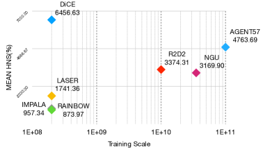
((a)) Mean

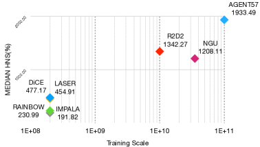
((b)) Median

Figure 1: Human Normalized Scores (%) of 57 games.

2 BACKGROUND

Consider an MDP, defined by a 5-tuple $(\mathcal{S},\mathcal{A},p,r,\gamma)$, where $\mathcal{S}$ is thee state space, $\mathcal{A}$ is the action space, $p$ is the state transition probability function which associates distributions over state to state-action pair, $r:\mathcal{S}\times\mathcal{A}\rightarrow\mathbb{R}$ is the reward function, and $\gamma\in(0,1)$ is the discounted factor. Let $\pi$ a distribution over action to each state be the policy.

The objective of reinforcement learning is to find

$$\operatorname*{arg\,max}_{\pi}\ \mathcal{J}_{\pi}=\mathbb{E}_{(s_{0},a_{0},s_{1},\ldots,s_{t},a_{t},\ldots)\sim\pi}\left[\sum_{k=0}^{\infty}\gamma^{k}r_{k}\right].$$ (1)

, where $\mathbb{E}_{(s_{0},a_{0},s_{1},\ldots,s_{t},a_{t},\ldots)\sim\pi}$ is a brief form of $\mathbb{E}_{a_{1}\sim\pi(a_{1}|s_{0}),s_{1}\sim p(s_{1}|a_{1},s_{0}),\ldots}$.

Value-based methods maximize $\mathcal{J}_{\pi}$ by generalized policy iteration (GPI) (Sutton, Barto, 2018). The policy evaluation is conducted by minimizing $\mathbb{E}_{\pi}[(\mathcal{T}Q^{\pi}-Q^{\pi})^{2}]$, where $\mathcal{T}Q^{\pi}$ is

$$\mathcal{T}Q^{\pi}(s_{t},a_{t}) =\mathbb{E}_{p}[r_{t}+\gamma V^{\pi}(s_{t})],$$

$$V^{\pi}(s_{t}) =\mathbb{E}_{\pi}[Q^{\pi}(s_{t},a_{t})]$$

where $\mathbb{E}_{p}$ is a shorthand of $\mathbb{E}_{s_{t+1}\sim p(s_{t+1}|s_{t},a_{t})}$ and $\mathbb{E}_{\pi}$ is a shorthand of $\mathbb{E}_{a_{t}\sim\pi(a_{t}|s_{t})}$. The policy improvement is usually achieved by $\epsilon$-greedy. A refined structure design of $Q^{\pi}$ is provided by dueling-Q (Wang et al., 2016). It estimates $Q^{\pi}$ by the summation of the advantage function and the state value function, $Q^{\pi}=A^{\pi}+V^{\pi}$.

When the large scale training is involved, the off-policy problem is inevitable. Denote $\mu$ as the behavior policy, $\pi$ as the target policy. $c_{t}\overset{def}{=}\min\{\frac{\pi_{t}}{\mu_{t}},\bar{c}\}$ is the clipped importance sampling. For brevity, $c_{[t:t+k]}\overset{def}{=}\prod_{i=0}^{k}c_{t+i}$. ReTrace (Munos et al., 2016) estimates $Q(s_{t},a_{t})$ by clipped per-step importance sampling

$$Q^{\tilde{\pi}}(s_{t},a_{t})=\mathbb{E}_{\mu}[Q(s_{t},a_{t})+\sum_{k\geq 0}\gamma^{k}c_{[t+1:t+k]}\delta^{Q}_{t+k}Q],$$ (2)

where $\delta^{Q}_{t}Q\overset{def}{=}r_{t}+\gamma Q(s_{t+1},a_{t+1})-Q(s_{t},a_{t})$. The ReTrace operator is a contraction mapping and has a fixed point $Q^{\tilde{\pi}_{ReTrace}}$ corresponding to some $\tilde{\pi}_{ReTrace}$. $Q^{\pi}$ is learned by minimizing $\mathbb{E}_{\mu}[(Q^{\tilde{\pi}}-Q^{\pi})^{2}]$, which gives the gradient ascent direction

$$\mathbb{E}_{\mu}[(Q^{\tilde{\pi}}-Q^{\pi})\nabla Q^{\pi}].$$ (3)

		HNS(%)		SABER(%)
	Num. Frames	Mean	Median	Mean	Median
DiCE	200M	6456.63	477.17	50.11	13.90
Rainbow	200M	873.97	230.99	28.39	4.92
IMPALA	200M	957.34	191.82	29.45	4.31
LASER	200M	1741.36	454.91	36.77	8.08
R2D2	10B	3374.31	1342.27	60.43	33.62
NGU	35B	3169.90	1208.11	50.47	21.19
Agent57	100B	4763.69	1933.49	76.26	43.62

Table 2: Atari Scores. Rainbow’s scores are from (Hessel et al., 2017). IMPALA’s scores are from (Espeholt et al., 2018). LASER’s scores are from (Schmitt et al., 2020), no sweep at 200M. R2D2’s scores are from (Kapturowski et al., 2018). NGU’s scores are from (Badia et al., 2020b). Agent57’s scores are from (Badia et al., 2020a).

Policy-based methods maximize $\mathcal{J}_{\pi}$ by policy gradient. It’s shown (Sutton, Barto, 2018) that $\nabla\mathcal{J}_{\pi}=\mathbb{E}_{\pi}[G\nabla\log\pi]$, where $G=\sum_{i=t}^{\infty}\gamma^{i}r_{i}$. When involved with an estimated baseline, it becomes an actor-critic algorithm. The policy gradient is given by $\nabla\mathcal{J}_{\pi}=\mathbb{E}_{\pi}[(G-V^{\pi})\nabla\log\pi]$, where $V^{\pi}$ is optimized by minimizing $\mathbb{E}_{\pi}[(G-V^{\pi})^{2}]$.

Since (Williams, Peng, 1991), many on-policy policy-based methods (Mnih et al., 2016b; Schulman et al., 2017b) add an entropy regularization to loss function like $\alpha\nabla\mathcal{H}(\pi)$, where $\mathcal{H}(\pi)=-\sum_{a^{\prime}}\pi(a^{\prime}|s)\log\pi(a^{\prime}|s)$ is the entropy of $\pi$.

As one large scale policy-based method, IMPALA (Espeholt et al., 2018) also introduces entropy. Besides, IMPALA introduces V-Trace off-policy actor-critic algorithm to correct the discrepancy between the target policy and the behavior policy. Let $\rho_{t}\overset{def}{=}\min\{\frac{\pi_{t}}{\mu_{t}},\bar{\rho}\}$, $c_{t}\overset{def}{=}\min\{\frac{\pi_{t}}{\mu_{t}},\bar{c}\}$ to be the clipped importance sampling. For brevity, let $c_{[t:t+k]}\overset{def}{=}\prod_{i=0}^{k}c_{t+i}$. V-Trace estimates $V(s_{t})$ by

$$V^{\tilde{\pi}}(s_{t})=\mathbb{E}_{\mu}[V(s_{t})+\sum_{k\geq 0}\gamma^{k}c_{[t:t+k-1]}\rho_{t+k}\delta^{V}_{t+k}V],$$ (4)

where $\delta^{V}_{t}V\overset{def}{=}r_{t}+\gamma V(s_{t+1})-V(s_{t})$. $V^{\pi}$ is learned by minimizing $\mathbb{E}_{\mu}[(V^{\tilde{\pi}}-V^{\pi})^{2}]$, giving the gradient ascent direction

$$\mathbb{E}_{\mu}[(V^{\tilde{\pi}}-V^{\pi})\nabla V^{\pi}].$$ (5)

If $\bar{c}\leq\bar{\rho}$, the V-Trace operator is a contraction mapping, and $V$ converges to $V^{\tilde{\pi}}$ that corresponds to

$$\tilde{\pi}(a|s)=\frac{\min\left\{\bar{\rho}\mu(a|s),\pi(a|s)\right\}}{\sum_{b\in\mathcal{A}}\min\left\{\bar{\rho}\mu(b|s),\pi(b|s)\right\}}.$$

Combining V-Trace into the Actor-Critic paradigm, the direction of the policy gradient is given by

$$\mathbb{E}_{\mu}\left[\rho_{t}(r_{t}+\gamma V^{\tilde{\pi}}(s_{t+1})-V(s_{t}))\nabla\log\pi\right].$$ (6)

Another related work is maximum entropy RL (Haarnoja et al., 2017, 2018a), which maximizes state value as well as the entropy of the policy. Here we call them MaxEnt. The objective of MaxEnt is to

$$maximize\ \mathcal{J}_{soft}=\mathbb{E}_{\pi}\left[\sum_{k=0}^{\infty}\gamma^{k}(r_{k}+\tau\textbf{H}[\pi])\right].$$

$Q^{\pi}_{soft}$ and $V^{\pi}_{soft}$ are defined by the soft Bellman equation

$$\mathcal{T}Q^{\pi}_{soft}(s_{t},a_{t})=\mathbb{E}_{p}[r_{t}+\gamma V^{\pi}_{soft}(s_{t+1})],$$ (7)

$$where V^{\pi}_{soft}(s_{t})=\mathbb{E}_{\pi}[Q^{\pi}_{soft}(s_{t},a_{t})-\tau\log\pi(a_{t}|s_{t})].$$

$\pi_{soft}$ is defined as a Boltzmann policy

$$\pi_{soft}(a_{t}|s_{t})\propto\exp((Q^{\pi}_{soft}(s_{t},a_{t})-V^{\pi}_{soft}(s_{t}))/\tau).$$

Although (Haarnoja et al., 2018a) achieves Adaptive Trade-off by adjusting $\tau$ adaptively, it still suffers some drawbacks. i) Since $\tau$ in $\mathcal{J}_{soft}$ encourages exploration by maximizing entropy reward when optimizing the target policy, it couples the exploration rate of the behavior policy with the target policy, which makes it neither Closed-form nor Diversity. ii) $\mathcal{J}_{soft}$ is regularized by H[$\pi$] compared to $\mathcal{J}_{\pi}$, which means the target policy is not Objective-invariant during training.

3 Method

In this section, we introduce DiCE and also check three characteristics. At the beginning of 3.1, we use $V_{\theta}$ to estimates $V^{\pi}$, $A_{\theta}$ to estimates $A^{\pi}$, $Q_{\theta}=V_{\theta}+A_{\theta}$ to estimate $Q^{\pi}$ and $\pi_{\theta}$ to approximate $\pi$, where $\theta$ represents all parameters to be optimized. But the target functions of $V_{\theta}$, $A_{\theta}$ and $Q_{\theta}$ will be changed later, which is detailed in 3.1. In 3.2 and 3.3, $V_{\theta}$, $A_{\theta}$ and $Q_{\theta}$ estimate the new target functions.

3.1 Closed-form Diversity

Assume $v_{\theta}\in\mathbb{R}^{|\mathcal{A}|}$ is a parameterized vector. For brevity, we write $v_{\theta}$ as $v$. Inspired by MaxEnt, we define a Boltzmann policy as

$$\pi_{\tau}(v)\propto\exp(v/\tau).$$

It’s evident that,

$$\textbf{H}[\pi_{\tau}]\to 0, \pi_{\tau}\to argmax, as\ \tau\to 0+;$$

$$\textbf{H}[\pi_{\tau}]\to\log|\mathcal{A}|, \pi_{\tau}\to uniform, as\ \tau\to+\infty.$$

Since $\textbf{H}[\pi_{\tau}]$ is a continuous function of $\tau$, for $\forall\ 0<e<\log|\mathcal{A}|$, $\exists\ \tau_{0}$ s.t. $\textbf{H}[\pi_{\tau_{0}}]=e$. So we can simply control $\textbf{H}[\pi_{\tau}]$ by choosing a proper $\tau$.

If we define a family of behavior policies as

$$\mathcal{B}_{v}=\{\pi_{\tau}(v)|\,\tau\in(0,+\infty)\},$$

it’s obvious that $\mathcal{B}_{v}$ is a family of closed-form functions of $v$ and $\mathcal{B}_{v}$ has one dimension of freedom $\tau$. So $\mathcal{B}_{v}$ achieves Closed-form Diversity for $v$.

Since the behavior policy is sampled from a family $\mathcal{B}_{v}$, it’s nature to ask what the definitions of $V^{\pi}$, $Q^{\pi}$ and $A^{\pi}$ are, i.e. what functions $V_{\theta}$, $Q_{\theta}$ and $A_{\theta}$ are estimating. As $(V^{\pi_{\tau}},Q^{\pi_{\tau}})$ satisfies the following Bellman equation,

$$\mathcal{T}Q^{\pi_{\tau}}_{t} =\mathbb{E}_{p}[r_{t}+\gamma V^{\pi_{\tau}}_{t+1}],$$

$$where\ V^{\pi_{\tau}}_{t} =\mathbb{E}_{a_{t}\sim\pi_{\tau}}[Q^{\pi_{\tau}}_{t}(\cdot,a_{t})],$$

we observe that $\tau$ only influences $(V^{\pi_{\tau}},Q^{\pi_{\tau}})$ when taking the expectation $V^{\pi_{\tau}}_{t}=\mathbb{E}_{\pi_{\tau}}[Q^{\pi_{\tau}}_{t}]$.

Assume $\tau$ is sampled from a distribution $\Omega$, the influence is totally eliminated as

$$\mathcal{T}Q^{\pi_{\tau}}_{t} =\mathbb{E}_{p}[r_{t}+\gamma V^{\pi_{\tau}}_{t+1}],$$

$$where\ V^{\pi_{\tau}}_{t} =\mathbb{E}_{\tau\sim\Omega}[\mathbb{E}_{a_{t}\sim\pi_{\tau}}[Q^{\pi_{\tau}}_{t}(\cdot,a_{t})]].$$

Now $Q^{\pi_{\tau}}_{t}$ only depends on the transition probability $p$ and the average policy $\pi_{\Omega}\overset{def}{=}\int_{\tau\sim\Omega}\pi_{\tau}$, which is free from $\tau$. Hence, we rewrite the above Bellman equation as

$$\mathcal{T}Q^{\Omega}_{t} =\mathbb{E}_{p}[r_{t}+\gamma V^{\Omega}_{t+1}],$$

$$where\ V^{\Omega}_{t} =\mathbb{E}_{a_{t}\sim\pi_{\Omega}}[Q^{\Omega}_{t}(\cdot,a_{t})],$$

where $Q^{\Omega}_{t}\overset{def}{=}\int_{\tau\sim\Omega}Q^{\pi_{\tau}}_{t}$, $V^{\Omega}_{t}\overset{def}{=}\int_{\tau\sim\Omega}V^{\pi_{\tau}}_{t}$. Similarly, we have $A^{\Omega}_{t}\overset{def}{=}\int_{\tau\sim\Omega}A^{\pi_{\tau}}_{t}$.

Now we use $V_{\theta}$ to estimates $V^{\Omega}$, $A_{\theta}$ to estimates $A^{\Omega}$, $Q_{\theta}=V_{\theta}+A_{\theta}$ to estimate $Q^{\Omega}$.

3.2 Objective-invariant Exploration

To check if $\mathcal{B}_{v}$ is Objective-invariant, by a typical derivative of cross entropy, we have $\nabla\log\pi_{\tau}=(\textbf{1}-\pi_{\tau})\frac{\nabla v}{\tau}$. Plugging into (6), we have the following policy gradient

$$\nabla\mathcal{J}_{\pi_{\tau}}=\mathbb{E}_{\mu_{\tau}}\left[\rho_{t}(r_{t}+\gamma V^{\tilde{\pi}_{\tau}}(s_{t+1})-V^{\pi_{\tau}}(s_{t}))(\textbf{1}-\pi_{\tau})\frac{\nabla v}{\tau}\right],$$

where ${\mu_{\tau}}$ is the behavior policy corresponding to ${\pi_{\tau}}$.

It’s obvious that $maximize\ \mathcal{J}_{\pi_{\tau}}$ is equivalent to $maximize\ \tau\mathcal{J}_{\pi_{\tau}}$. Taking an additional $\tau$, we free the scale of policy gradient from $\tau$,

$$\nabla\tau\mathcal{J}_{\pi_{\tau}}=\mathbb{E}_{\mu_{\tau}}\left[\rho_{t}(r_{t}+\gamma V^{\tilde{\pi}_{\tau}}(s_{t+1})-V^{\pi_{\tau}}(s_{t}))(\textbf{1}-\pi_{\tau})\nabla v\right].$$

Taking expectation w.r.t. $\tau$, we have

$$\nabla\mathbb{E}_{\tau\sim\Omega}[\tau\mathcal{J}_{\pi_{\tau}}]=\mathbb{E}_{\tau\sim\Omega}\left[\mathbb{E}_{\mu_{\tau}}\left[\rho_{t}(r_{t}+\gamma V^{\tilde{\pi}_{\tau}}(s_{t+1})-V^{\pi_{\tau}}(s_{t}))(\textbf{1}-\pi_{\tau})\nabla v\right]\right].$$ (8)

When the importance sampling clip $\bar{\rho}$ and $\bar{c}$ is $+\infty$, we know V-Trace is an unbiased estimation (Espeholt et al., 2018). Regardless the function approximation error of $V_{\theta}$, we have

$$\nabla\mathbb{E}_{\tau\sim\Omega}[\tau\mathcal{J}_{\pi_{\tau}}]=\mathbb{E}_{\tau\sim\Omega}\left[\mathbb{E}_{\pi_{\tau}}\left[A^{\pi_{\tau}}(\textbf{1}-\pi_{\tau})\nabla v\right]\right].$$

Therefore, if $\Omega$ is a fixed distribution of $\tau$, $\mathcal{B}_{v}$ is Objective-invariant as $\mathbb{E}_{\tau\sim\Omega}[\tau\mathcal{J}_{\pi_{\tau}}]$ is free from $\tau$. If $\Omega$ can be optimized, let $\tau_{0}=\operatorname*{arg\,max}_{\tau}\{\tau\mathcal{J}_{\pi_{\tau}}\}$, then $\mathbb{E}_{\tau\sim\Omega}[\tau\mathcal{J}_{\pi_{\tau}}]=\tau_{0}\mathcal{J}_{\pi_{\tau_{0}}}$ is equivalent to the objective defined in (1). So it’s also $\tau$-free.

In practice, we choose $v=A_{\theta}$, this is because (Schulman et al., 2017a) proves the equivalence between the evaluation of the state-action value function and the policy gradient with the evaluation of the state value function. But it’s an open question if there exists a better choice of $v$.

We use the Learner-Actor architecture. The Actor part of DiCE is shown in Algorithm 1, and the full version can be found in appendix B.

Algorithm 1 DiCE Algorithm (Actor).

  Initialize Parameter Server (PS) and Data Collector (DC).

  // ACTOR

  Initialize $d_{pull}$, $M$, $\Omega$.

  Initialize $\theta$, i.e. initialize $A_{\theta}$, $V_{\theta}$,$Q_{\theta}=V_{\theta}+A_{\theta}$ and $\pi_{\theta}$.

  Initialize $\{\mathcal{B}_{m}\}_{m=1,...,M}$ and sample $\tau\sim\Omega$.

  Initialize $count=0$, $G=0$.

  Initialize environment and $s=s_{0}$.

  while $True$ do

     Calculate $\pi_{\tau}(\cdot|s)\propto\exp(A_{\theta}/\tau)$.

     Sample $a\sim\pi_{\tau}(\cdot|s)$.

     $s,r,done\sim p(\cdot|s,a)$.

     $G\leftarrow G+r$.

     if $done$ then

        Update $\Omega$ by $(\tau,G)$.

        Send data to DC.

        Sample $\tau\sim\Omega$.

        $G\leftarrow 0$.

        Reset the environment and $s=s_{0}$.

     end if

     if $count\mod d_{pull}$ = 0 then

        Pull $\theta$ from PS and update $\theta$.

     end if

     $count\leftarrow count+1$.

  end while

3.3 Adaptive Trade-off

In Algorithm 1, both "Update $\Omega$ by $(\tau,G)$" and "Sample $\tau\sim\Omega$" are achieved by Adaptive Trade-off.

In practice, we use a Bandits Vote Algorithm (BVA) to adaptively update $\Omega$ to maximize the expected cumulative return. Different from other meta-controllers, BVA uses an ensemble of bandits. During the training process, each bandit is updated individually. During the evaluation process, each bandit provides one evaluation for each $\tau$ and the final evaluation of each $\tau$ is the average evaluation of all bandits. During the sample process, each bandit provides several candidates and one candidate is sampled uniformly from all candidates. The details of BVA is shown in Appendix A.

4 Experiments

We firstly introduce our basic setup. Then we report our results on ALE, namely, 57 atari games. In our ablation study, we report the results of the policy-based baseline of DiCE, which shows that DiCE boosts our policy-based baseline by a large margin. We also make additional ablation study to check the effect of the proposed characteristics.

4.1 Basic Setup

All the experiment is accomplished using 92 CPU cores and a single Tesla-V100-SXM2-32GB GPU. To deal with partially observable MDP (POMDP), we use a recurrent encoder by LSTM (Schmidhuber, 1997) with 256 units. We use burn-in (Kapturowski et al., 2018) to deal with representational drift. We store the recurrent state during inference and make it the start point of the burn-in phase. We train each sample twice. We do not use any intrinsic reward in any experiment. To be general, we will not end the episode if life is lost.

We use BVA to sample $\tau$s, evaluate $\tau$s and find the best region of $\tau$s. We use $\tau$s sampled from the best region to evaluate the expected return. Hyperparameters are listed in Appendix C.

4.2 Analysis and Summary of Results

Table 2 summarizes the mean and the median Human Normalized Scores (HNS) of 57 games, as well as Standardized Atari BEnchmark for RL (SABER)(Toromanoff et al., 2019). Scores of 57 games and learning curves are listed in Appendix E. The videos will be released in the future.

In general, DiCE achieves SOTA on mean HNS compared to other algorithms, including 10B+ algorithms. DiCE also achieves the highest median HNS among 200M algorithms.

The results can roughly be classified into three kinds: (i) results of some games achieve historical highest score, such as Atlantis, Gopher, Jamesbond. For fairness, we also report mean and median SABER, which is normalized by Human World Records and capped by 200%. The mean SABER is very competitive compared to other 10B+ algorithms. The mean SABER and median SABER is much higher than other 200M algorithms, which shows the overall performance is much better than other 200M algorithms. (ii) results of some games are increasing and the learning processes have not converged, such as Alien, BeamRider, ChopperCommand; (iii) results of some games encounter the bottleneck due to the hard exploration problem, such as IceHockey, PrivateEye, Surround.

One crucial thing for solving (iii) is how to acquire better samples. Even DiCE achieves controlling the entropy of the behavior policy in a Closed-form, DiCE only maintains one dimension of freedom. DiCE tries to collect diverse samples by enlarging the behavior policy to a family of policies $\{\pi_{\tau}\}_{\tau\in[K,+\infty]}$. The family can achieve a large range of entropy. However, it’s obvious that $\pi_{\tau}$ is an order-preserving mapping of $A$, which means that the total order relations of actions’ probability distributions are identical for $\forall\ \pi_{\tau}\in\{\pi_{\tau}\}_{\tau\in[K,+\infty]}$. Value-based methods such as R2D2 collect samples by a family of policies $\{\pi_{\epsilon}\}_{\epsilon\in[0,1]}$, where $\pi_{\epsilon}$ represents $\epsilon$-greedy. Except for the max $Q$-value, $\pi_{\epsilon}$ does not preserve the order. $\{\pi_{\epsilon}\}_{\epsilon\in[0,1]}$ is more likely to explore the state where $\{\pi_{\tau}\}_{\tau\in[K,+\infty]}$ less prefers. The data distribution of samples is influenced by the inductive bias induced by the family of behavior policies. It’s critical and open to define a proper family of closed-form functions for more elite samples. Instead, NGU and Agent57 achieve active exploration of the environment by the intrinsic reward. Such exploration enlarges MDP, so UVFA (Schaul et al., 2015) is needed.

DiCE focuses on Objective-invariant Exploration. There are some hints to improve DiCE. The first is to enlarge the function space of the behavior policy by a linear combination. Since $\pi_{\epsilon}$ is identical to $\epsilon\cdot\pi_{\tau\rightarrow+\infty}+(1-\epsilon)\cdot\pi_{\tau\rightarrow 0+}$, it’s reasonable to consider a combination representation for a larger family of behavior policies, such as $\{\sum_{i}\alpha_{i}\cdot\pi_{\tau_{i}}|\sum_{i}\alpha_{i}=1\}$. The second is to adopt the idea of LASER by shared experience replay, which gives diverse samples from different families of policies $\{\{\pi_{n,\tau}\}_{\tau\in[K,+\infty]}\}_{n=1,2,...}$. The third is to make a better policy evaluation. Now the value function $V_{\theta}$ is estimating the average policy $\pi_{\Omega}$, which is $V^{\Omega}$. A better way is to use a UVFA or a closed-form expression, if exists, to estimate $\{V^{\pi_{\tau}}\}_{\tau\in[K,+\infty]}$.

4.3 Ablation Study

We firstly provide the scores of the baseline on 57 atari games. All hyperparameters of the baseline are the same as DiCE. Except for that we remove "Update $\Omega$ by $(\tau,G)$" and change "Sample $\tau\sim\Omega$" to "$\tau=1$" in Algorithm 1, the baseline is trained and evaluated identically to DiCE. From another perspective, we apply DiCE directly on the baseline without any change.

		HNS(%)		SABER(%)
	Num. Frames	Mean	Median	Mean	Median
DiCE	200M	6456.63	477.17	50.11	13.90
baseline	200M	1929.95	195.54	35.91	8.73

Table 3: Comparison to baseline.

The summary is shown in Table 3. Full comparison on 57 games are listed in Appendix D. The progress is impressive. DiCE promotes mean HNS by $235\%$, median HNS by $145\%$, mean SABER by $40\%$ and median SABER by $59\%$. Recalling Table 2, although our baseline meets SOTA performance, there is no evident performance difference between our baseline and other 200M algorithms. But DiCE achieves the best performance on all criteria among 200M algorithm and is approaching 10B+ algorithms on some criteria. This phenomenon proves that DiCE is very effective and boosts our policy-based baseline to a new State-Of-The-Art.

Name	Characteristics
DiCE	Closed-form Diversity, Objective-invariant Exploration, Adaptive Trade-off
baseline	N/A
random	Closed-form Diversity, Objective-invariant Exploration
entropy	Closed-form Diversity, Adaptive Trade-off

Table 4: Ablation Settings.

We make additional ablation study to find how much each characteristic contributes to DiCE. To check Objective-invariant, we add an entropy regularization with coefficient = 1 to the loss function, named as entropy. To check Adaptive Trade-off, we remove "Update $\Omega$ by $(\tau,G)$" in Algorithm 1, which means the distribution of $\tau$ is always the fixed initial distribution, named as random. It’s impossible to check Closed-form Diversity solely. If Closed-form Diversity does not hold, there is no need to consider Objective-invariant Exploration and Adaptive Trade-off.

We choose Breakout and ChopperCommand to do ablation study, because the performances of DiCE and the baseline on these two games are comparable.

((a)) breakout

((b)) chopper_command

Figure 2: Evaluation Return Curves.

The evaluation curve are shown in Figure 2. It’s obvious that random performs the worst, which evidently proves that Adaptive Trade-off is critical in DiCE. On the early stage of Breakout, DiCE and entropy show a higher sample efficiency that baseline and random. Notice that DiCE and entropy have Adaptive Trade-off, while baseline and random do not. We see Adaptive Trade-Off helps boosting the sample efficiency. There is no significant difference between DiCE and entropy, as DiCE performs better on ChopperCommand but worse on Breakout. So we cannot make a conclusion whether Objective-invariant is better or not. As for Closed-form Diversity, the full comparison between DiCE and baseline has already shown that DiCE is effective. Since Closed-form Diversity is the necessary condition for DiCE, there is no doubt that Closed-form Diversity is important. In general, we conclude that Closed-form Diversity and Adaptive Trade-off are critical. As for Objective-invariant Exploration, it’s uncertain whether Objective-invariant is better, but Exploration is one of the most important thing in RL.

Although DiCE enlarges the behavior policy to a family of behavior policies, it’s still a question to find what a good exploration is. DisCor (Kumar et al., 2020) has claimed that the choice of the sampling distribution is of crucial importance for the stability and efficiency of ADP algorithms. With a given replay buffer, DisCor re-weights each sample to mitigate this phenomenon. But if working on sample acquiring rather than sample re-weighting, it’s an interesting question to find a proper family of behavior policies such that the target policy learned with collected samples can achieve higher sample efficiency. Meanwhile, the superiority of this proper family of the behavior policies should be guaranteed. We leave this question for future study.

5 Conclusion

This paper proposes three characteristics, Closed-form Diversity, Objective-invariant Exploration and Adaptive Trade-off. We propose a mechanism for policy-based methods that enjoys three characteristics. The mechanism is sample efficient and boosts policy-based baseline to State-Of-The-Art with 200M training scale. The overall performance is higher than other 200M algorithms and is competitive compared to 10B+ algorithms. We analyse the ablation cases and discuss the potential improvement in future work.

Appendix A Bandit Vote Algorithm

The algorithm is shown in Algorithm 2.

Algorithm 2 Bandits Vote Algorithm.

  for $m=1,...,M$ do

     Sample $mode\sim\{argmax,random\}$, sample $lr$, sample $width$.

     Initialize $B_{m}=Bandit(mode,l,r,acc,width,lr,\textbf{w},\textbf{N},d)$.

  end for

  while $True$ do

     for $m=1,...,M$ do

        Evaluate $\mathcal{B}_{m}$ by (9).

        Sample candidates $c_{m,1},...,c_{m,d}$ by $mode$ and (11) from $\mathcal{B}_{m}$.

     end for

     Sample $x$ from $\{c_{m,i}\}_{m=1,...,M;i=1,...,d}$.

     Execute $x$ and receive $g$.

     for $m=1,...,M$ do

        Update $\mathcal{B}_{m}$ with $(x,g)$ by (10).

     end for

  end while

Let’s firstly define a bandit as $\mathcal{B}=Bandit(mode,l,r,acc,width,lr,\textbf{w},\textbf{N},d)$.

• $mode$ is the mode of sampling, with two choices, $argmax$ and $random$.

• $l$ is the left boundary of $\mathcal{B}$, and each $x$ is clipped to $x=\max\{x,l\}$.

• $r$ is the right boundary of $\mathcal{B}$, and each $x$ is clipped to $x=\min\{x,r\}$.

• $acc$ is the accuracy, where each $x$ is located in the $\lfloor(\min\{\max\{x,l\},r\}-l)/acc\rfloor$th tile.

• $width$ is the tile coding width, where the value of the $i$th tile is estimated by the average of $\{\textbf{w}_{i-width},...,\textbf{w}_{i+width}\}$.

• $lr$ is the learning rate.

• w is a vector in $\mathbb{R}^{\lfloor(r-l)/acc\rfloor}$, which represents the weight of each tile.

• N is a vector in $\mathbb{R}^{\lfloor(r-l)/acc\rfloor}$, which counts the number of sampling of each tile.

• $d$ is an integer, which represents how many candidates is provided by $\mathcal{B}$ when sampling.

During the evaluation process, we evaluate the value of the $i$th tile by

$$V_{i}=\frac{1}{2*width+1}\sum_{k=i-width}^{i+width}\textbf{w}_{k}.$$ (9)

During the training process, for each sample $(x,g)$, where $g$ is the target value. Since $x$ locates in the $i$th tile, we update $\mathcal{B}$ by

$$\left\{\begin{aligned} &i=\lfloor(\min\{\max\{x,l\},r\}-l)/acc\rfloor,\\ &\textbf{w}_{j}\leftarrow\textbf{w}_{j}+lr*\left(g-V_{i}\right),j=i-width,...,i+width,\\ &\textbf{N}_{i}\leftarrow\textbf{N}_{i}+1.\end{aligned}\right.$$ (10)

During the sampling process, we firstly evaluate $\mathcal{B}$ by (9) and get $(V_{1},...,V_{\lfloor(r-l)/acc\rfloor})$. We calculate the score of $i$th tile by

$$score_{i}=\frac{V_{i}-\mu(\{V_{j}\}_{j=1,...,\lfloor(r-l)/acc\rfloor})}{\sigma(\{V_{j}\}_{j=1,...,\lfloor(r-l)/acc\rfloor})}+c\cdot\sqrt{\frac{\log(1+\sum_{j}\textbf{N}_{j})}{1+\textbf{N}_{i}}}.$$ (11)

For different $mode$s, we sample the candidates by the following mechanism,

• if $mode$ = $argmax$, find tiles with top-$d$ $score$s, then sample $d$ candidates from these tiles, one uniformly from a tile;

• if $mode$ = $random$, sample $d$ tiles with $score$s as the logits without replacement, then sample $d$ candidates from these tiles, one uniformly from a tile;

In practice, we define a set of bandits $\{\mathcal{B}_{m}\}_{m=1,...,M}$. At each step, we sample $d$ candidates $\{c_{m,i}\}_{i=1,...,d}$ from each $B_{m}$, so we have a set of $m\times d$ candidates $\{c_{m,i}\}_{m=1,...,M;i=1,...,d}$. Then we sample uniformly from these $m\times d$ candidates to get $x$. At last, we transform the selected $x$ to $\tau$ by $\tau=\frac{1}{\exp(x)-1}$. When we receive $(\tau,g)$, we transform $\tau$ to $x$ by $x=\log(1+1/\tau)$. Then we update each $B_{m}$ by (10).

Appendix B Full Algorithm

Algorithm 3 DiCE Algorithm full version.

  Initialize Parameter Server (PS) and Data Collector (DC).

  

  // LEARNER

  Initialize $d_{push}$.

  Initialize $\theta$, i.e. initialize $A_{\theta}$, $V_{\theta}$, $Q_{\theta}=V_{\theta}+A_{\theta}$.

  Initialize $\pi_{\tau}\propto\exp(A_{\theta}/\tau)$.

  Initialize $count=0$.

  while $True$ do

     Load data from DC.

     Estimate $Q^{\pi}$ and $V^{\pi}$ by proper off-policy algorithms.

         (For instance, ReTrace (2) for $Q^{\pi}$ and V-Trace (4) for $V^{\pi}$.)

     Update $\theta$ by policy gradient (8) and policy evaluation (3), (5).

     if $count$ mod $d_{push}$ = 0 then

        Push $\theta$ to PS.

     end if

     $count\leftarrow count+1$.

  end while

  

  // ACTOR

  Initialize $d_{pull}$, $M$, $\Omega$.

  Initialize $\theta$, i.e. initialize $A_{\theta}$, $V_{\theta}$,$Q_{\theta}=V_{\theta}+A_{\theta}$ and $\pi_{\theta}$.

  Initialize $\{\mathcal{B}_{m}\}_{m=1,...,M}$ and sample $\tau\sim\Omega$.

  Initialize $count=0$, $G=0$.

  Initialize environment and $s=s_{0}$.

  while $True$ do

     Calculate $\pi_{\tau}(\cdot|s)\propto\exp(A_{\theta}/\tau)$.

     Sample $a\sim\pi_{\tau}(\cdot|s)$.

     $s,r,done\sim p(\cdot|s,a)$.

     $G\leftarrow G+r$.

     if $done$ then

        Update $\Omega$ by $(\tau,G)$.

        Send data to DC.

        Sample $\tau\sim\Omega$.

        $G\leftarrow 0$.

        Reset the environment and $s=s_{0}$.

     end if

     if $count\mod d_{pull}$ = 0 then

        Pull $\theta$ from PS and update $\theta$.

     end if

     $count\leftarrow count+1$.

  end while

Appendix C Hyperparameters

Parameter	Value
Image Size	(84, 84)
Grayscale	Yes
Num. Action Repeats	4
Num. Frame Stacks	4
Action Space	Full
End of Episode When Life Lost	No
Num. States	200M
Sample Reuse	2
Num. Environments	160
Reward Shape	$\log(abs(r)+1.0)\cdot(2\cdot 1_{\{r\geq 0\}}-1_{\{r<0\}})$
Reward Clip	No
Intrinsic Reward	No
Random No-ops	30
Burn-in	40
Seq-length	80
Burn-in Stored Recurrent State	Yes
Bootstrap	Yes
Batch size	64
Discount ($\gamma$)	0.997
$V$-loss Scaling ($\xi$)	1.0
$Q$-loss Scaling ($\alpha$)	10.0
$\pi$-loss Scaling ($\beta$)	10.0
Entropy Regularization	No
Importance Sampling Clip $\bar{c}$	1.05
Importance Sampling Clip $\bar{\rho}$	1.05
Backbone	IMPALA,deep
LSTM Units	256
Optimizer	Adam Weight Decay
Weight Decay Rate	0.01
Weight Decay Schedule	Anneal linearly to 0
Learning Rate	5e-4
Warmup Steps	4000
Learning Rate Schedule	Anneal linearly to 0
AdamW $\beta_{1}$	0.9
AdamW $\beta_{2}$	0.98
AdamW $\epsilon$	1e-6
AdamW Clip Norm	50.0
Learner Push Model Every $n$ Steps	25
Actor Pull Model Every $n$ Steps	64
Num. Bandits	7
Bandit Learning Rate	Uniform([0.05, 0.1, 0.2])
Bandit Tiling Width	Uniform([1, 2, 3])
Num. Bandit Candidates	7
Bandit Value Normalization	Yes
Bandit UCB Scaling	1.0
Bandit Search Range for $1/\tau$	[0.0, 50.0]

Table 5: Hyperparameters for Atari Experiments.

Appendix D Comparison to Baseline

Games	RND	HUMAN	BASELINE	HNS(%)	DiCE	HNS(%)
Scale			200M		200M
alien	227.8	7127.8	13720	195.54	10641	150.92
amidar	5.8	1719.5	560	32.34	653.9	37.82
assault	222.4	742	16228	3080.37	36251	6933.91
asterix	210	8503.3	213580	2572.80	851210	10261.30
asteroids	719	47388.7	18621	38.36	759170	1625.15
atlantis	12850	29028.1	3211600	19772.10	3670700	22609.89
bank heist	14.2	753.1	895.3	119.24	1381	184.98
battle zone	236	37187.5	70137	189.17	130410	352.28
beam rider	363.9	16926.5	34920	208.64	104030	625.90
berzerk	123.7	2630.4	1648	60.81	1222	43.81
bowling	23.1	160.7	162.4	101.24	176.4	111.41
boxing	0.1	12.1	98.3	818.33	99.9	831.67
breakout	1.7	30.5	624.3	2161.81	696	2410.76
centipede	2090.9	12017	102600	1012.57	38938	371.21
chopper command	811	7387.8	616690	9364.42	41495	618.60
crazy climber	10780.5	36829.4	161250	600.70	157250	584.73
defender	2874.5	18688.9	421600	2647.75	837750	5279.21
demon attack	152.1	1971	291590	16022.76	549450	30199.46
double dunk	-18.6	-16.4	20.25	1765.91	23	1890.91
enduro	0	860.5	10019	1164.32	14317	1663.80
fishing derby	-91.7	-38.8	53.24	273.99	48.8	265.60
freeway	0	29.6	3.46	11.69	33.7	113.85
frostbite	65.2	4334.7	1583	35.55	8102	188.24
gopher	257.6	2412.5	188680	8743.90	454150	21063.27
gravitar	173	3351.4	4311	130.19	6150	188.05
hero	1027	30826.4	24236	77.88	17655	55.80
ice hockey	-11.2	0.9	1.56	105.45	-8.1	25.62
jamesbond	29	302.8	12468	4543.10	567020	207082.18
kangaroo	52	3035	5399	179.25	14286	477.17
krull	1598	2665.5	64347	5878.13	11104	890.49
kung fu master	258.5	22736.3	124630.1	553.31	1270800	5652.43
montezuma revenge	0	4753.3	2488.4	52.35	2528	53.18
ms pacman	307.3	6951.6	7579	109.44	4296	60.03
name this game	2292.3	8049	32098	517.76	30037	481.95
phoenix	761.5	7242.6	498590	7681.23	597580	9208.60
pitfall	-229.4	6463.7	-17.8	3.16	-21.8	3.10
pong	-20.7	14.6	20.39	116.40	21	118.13
private eye	24.9	69571.3	134.1	0.16	15095	21.67
qbert	163.9	13455.0	21043	157.09	19091	142.40
riverraid	1338.5	17118.0	11182	62.38	17081	99.77
road runner	11.5	7845	251360	3208.64	57102	728.80
robotank	2.2	11.9	10.44	84.95	69.7	695.88
seaquest	68.4	42054.7	11862	28.09	2728	6.33
skiing	-17098	-4336.9	-12730	34.23	-9327	60.90
solaris	1236.3	12326.7	2319	9.76	3653	21.79
space invaders	148	1668.7	3031	189.58	105810	6948.25
star gunner	664	10250	337150	3510.18	358650	3734.47
surround	-10	6.5	-10	0.00	-9.8	1.21
tennis	-23.8	-8.3	-21.05	17.74	23.7	306.45
time pilot	3568	5229.2	84341	4862.62	150930	8871.35
tutankham	11.4	167.6	381	236.62	380.3	236.17
up n down	533.4	11693.2	416020	3723.06	907170	8124.13
venture	0	1187.5	0	0.00	1969	165.81
video pinball	0	17667.9	297920	1686.22	673840	3813.92
wizard of wor	563.5	4756.5	26008	606.83	21325	495.15
yars revenge	3092.9	54576.9	76903.5	143.37	84684	158.48
zaxxon	32.5	9173.3	46070.8	503.66	62133	679.38
MEAN HNS(%)	0.00	100.00		1929.95		6456.63
MEDIAN HNS(%)	0.00	100.00		195.54		477.17

Games	RND	HWR	BASELINE	SABER(%)	DiCE	SABER(%)
Scale			200M		200M
alien	227.8	251916	13729	5.36	10641	4.14
amidar	5.8	104159	560	0.53	653.9	0.62
assault	222.4	8647	16228	189.99	36251	200.00
asterix	210	1000000	213580	21.34	851210	85.12
asteroids	719	10506650	18621	0.17	759170	7.22
atlantis	12850	10604840	3211600	30.20	3670700	34.53
bank heist	14.2	82058	895.3	1.07	1381	1.67
battle zone	236	801000	70137	8.73	130410	16.26
beam rider	363.9	999999	34920	3.46	104030	10.37
berzerk	123.7	1057940	1648	0.14	1222	0.10
bowling	23.1	300	162.4	50.31	176.4	55.36
boxing	0.1	100	98.3	98.30	99.9	99.90
breakout	1.7	864	624.3	72.20	696	80.52
centipede	2090.9	1301709	102600	7.73	38938	2.84
chopper command	811	999999	616690	61.64	41495	4.07
crazy climber	10780.5	219900	161250	71.95	157250	70.04
defender	2874.5	6010500	421600	6.97	837750	13.90
demon attack	152.1	1556345	291590	18.73	549450	35.30
double dunk	-18.6	21	20.25	98.11	23	105.05
enduro	0	9500	10019	105.46	14317	150.71
fishing derby	-91.7	71	53.24	89.08	48.8	86.36
freeway	0	38	3.46	9.11	33.7	88.68
frostbite	65.2	454830	1583	0.33	8102	1.77
gopher	257.6	355040	188680	53.11	454150	127.94
gravitar	173	162850	4311	2.54	6150	3.67
hero	1027	1000000	24236	2.32	17655	1.66
ice hockey	-11.2	36	1.56	27.03	-8.1	6.57
jamesbond	29	45550	12468	27.33	567020	200.00
kangaroo	52	1424600	5399	0.38	14286	1.00
krull	1598	104100	64347	61.22	11104	9.27
kung fu master	258.5	1000000	124630.1	12.44	1270800	127.09
montezuma revenge	0	1219200	2488.4	0.20	2528	0.21
ms pacman	307.3	290090	7579	2.51	4296	1.38
name this game	2292.3	25220	32098	130.00	30037	121.01
phoenix	761.5	4014440	498590	12.40	597580	14.87
pitfall	-229.4	114000	-17.8	0.19	-21.8	0.18
pong	-20.7	21	20.39	98.54	21	100.00
private eye	24.9	101800	134.1	0.11	15095	14.81
qbert	163.9	2400000	21043	0.87	19091	0.79
riverraid	1338.5	1000000	11182	0.99	17081	1.58
road runner	11.5	2038100	251360	12.33	57102	2.80
robotank	2.2	76	10.44	11.17	69.7	91.46
seaquest	68.4	999999	11862	1.18	2728	0.27
skiing	-17098	-3272	-12730	31.59	-9327	56.21
solaris	1236.3	111420	2319	0.98	3653	2.19
space invaders	148	621535	3031	0.46	105810	17.00
star gunner	664	77400	337150	200.00	358650	200.00
surround	-10	9.6	-10	0.00	-9.8	1.02
tennis	-23.8	21	-21.05	6.14	23.7	106.03
time pilot	3568	65300	84341	130.84	150930	200.00
tutankham	11.4	5384	381	6.88	380.3	6.87
up n down	533.4	82840	416020	200.00	907170	200.00
venture	0	38900	0	0.00	1969	5.06
video pinball	0	89218328	297920	0.33	673840	0.76
wizard of wor	563.5	395300	26008	6.45	21325	5.26
yars revenge	3092.9	15000105	76903.5	0.49	84684	0.54
zaxxon	32.5	83700	46070.8	55.03	62133	74.22
MEAN SABER(%)	0.00	100.00		35.91		50.11
MEDIAN SABER(%)	0.00	100.00		8.73		13.90

Appendix E Atari Results

E.1 Atari Games Table of Scores Based on Human Average Records

Random scores and average human’s scores are from (Badia et al., 2020a). Rainbow’s scores are from (Hessel et al., 2017). IMPALA’s scores are from (Espeholt et al., 2018). LASER’s scores are from (Schmitt et al., 2020), no sweep at 200M. As there are many versions of R2D2 and NGU, we use original papers’. R2D2’s scores are from (Kapturowski et al., 2018). NGU’s scores are from (Badia et al., 2020b). Agent57’s scores are from (Badia et al., 2020a).

Games	RND	HUMAN	RAINBOW	HNS(%)	IMPALA	HNS(%)	LASER	HNS(%)	DiCE	HNS(%)
Scale			200M		200M		200M		200M
alien	227.8	7127.8	9491.7	134.26	15962.1	228.03	35565.9	512.15	10641	150.92
amidar	5.8	1719.5	5131.2	299.08	1554.79	90.39	1829.2	106.4	653.9	37.82
assault	222.4	742	14198.5	2689.78	19148.47	3642.43	21560.4	4106.62	36251	6933.91
asterix	210	8503.3	428200	5160.67	300732	3623.67	240090	2892.46	851210	10261.30
asteroids	719	47388.7	2712.8	4.27	108590.05	231.14	213025	454.91	759170	1625.15
atlantis	12850	29028.1	826660	5030.32	849967.5	5174.39	841200	5120.19	3670700	22609.89
bank heist	14.2	753.1	1358	181.86	1223.15	163.61	569.4	75.14	1381	184.98
battle zone	236	37187.5	62010	167.18	20885	55.88	64953.3	175.14	130410	352.28
beam rider	363.9	16926.5	16850.2	99.54	32463.47	193.81	90881.6	546.52	104030	625.90
berzerk	123.7	2630.4	2545.6	96.62	1852.7	68.98	25579.5	1015.51	1222	43.81
bowling	23.1	160.7	30	5.01	59.92	26.76	48.3	18.31	176.4	111.41
boxing	0.1	12.1	99.6	829.17	99.96	832.17	100	832.5	99.9	831.67
breakout	1.7	30.5	417.5	1443.75	787.34	2727.92	747.9	2590.97	696	2410.76
centipede	2090.9	12017	8167.3	61.22	11049.75	90.26	292792	2928.65	38938	371.21
chopper command	811	7387.8	16654	240.89	28255	417.29	761699	11569.27	41495	618.60
crazy climber	10780.5	36829.4	168788.5	630.80	136950	503.69	167820	626.93	157250	584.73
defender	2874.5	18688.9	55105	330.27	185203	1152.93	336953	2112.50	837750	5279.21
demon attack	152.1	1971	111185	6104.40	132826.98	7294.24	133530	7332.89	549450	30199.46
double dunk	-18.6	-16.4	-0.3	831.82	-0.33	830.45	14	1481.82	23	1890.91
enduro	0	860.5	2125.9	247.05	0	0.00	0	0.00	14317	1663.80
fishing derby	-91.7	-38.8	31.3	232.51	44.85	258.13	45.2	258.79	48.8	265.60
freeway	0	29.6	34	114.86	0	0.00	0	0.00	33.7	113.85
frostbite	65.2	4334.7	9590.5	223.10	317.75	5.92	5083.5	117.54	8102	188.24
gopher	257.6	2412.5	70354.6	3252.91	66782.3	3087.14	114820.7	5316.40	454150	21063.27
gravitar	173	3351.4	1419.3	39.21	359.5	5.87	1106.2	29.36	6150	188.05
hero	1027	30826.4	55887.4	184.10	33730.55	109.75	31628.7	102.69	17655	55.80
ice hockey	-11.2	0.9	1.1	101.65	3.48	121.32	17.4	236.36	-8.1	25.62
jamesbond	29	302.8	19809	72.24	601.5	209.09	37999.8	13868.08	567020	207082.18
kangaroo	52	3035	14637.5	488.05	1632	52.97	14308	477.91	14286	477.17
krull	1598	2665.5	8741.5	669.18	8147.4	613.53	9387.5	729.70	11104	890.49
kung fu master	258.5	22736.3	52181	230.99	43375.5	191.82	607443	2701.26	1270800	5652.43
montezuma revenge	0	4753.3	384	8.08	0	0.00	0.3	0.01	2528	53.18
ms pacman	307.3	6951.6	5380.4	76.35	7342.32	105.88	6565.5	94.19	4296	60.03
name this game	2292.3	8049	13136	188.37	21537.2	334.30	26219.5	415.64	30037	481.95
phoenix	761.5	7242.6	108529	1662.80	210996.45	3243.82	519304	8000.84	597580	9208.60
pitfall	-229.4	6463.7	0	3.43	-1.66	3.40	-0.6	3.42	-21.8	3.10
pong	-20.7	14.6	20.9	117.85	20.98	118.07	21	118.13	21	118.13
private eye	24.9	69571.3	4234	6.05	98.5	0.11	96.3	0.10	15095	21.67
qbert	163.9	13455.0	33817.5	253.20	351200.12	2641.14	21449.6	160.15	19091	142.40
riverraid	1338.5	17118.0	22920.8	136.77	29608.05	179.15	40362.7	247.31	17081	99.77
road runner	11.5	7845	62041	791.85	57121	729.04	45289	578.00	57102	728.80
robotank	2.2	11.9	61.4	610.31	12.96	110.93	62.1	617.53	69.7	695.88
seaquest	68.4	42054.7	15898.9	37.70	1753.2	4.01	2890.3	6.72	2728	6.33
skiing	-17098	-4336.9	-12957.8	32.44	-10180.38	54.21	-29968.4	-100.86	-9327	60.90
solaris	1236.3	12326.7	3560.3	20.96	2365	10.18	2273.5	9.35	3653	21.79
space invaders	148	1668.7	18789	1225.82	43595.78	2857.09	51037.4	3346.45	105810	6948.25
star gunner	664	10250	127029	1318.22	200625	2085.97	321528	3347.21	358650	3734.47
surround	-10	6.5	9.7	119.39	7.56	106.42	8.4	111.52	-9.8	1.21
tennis	-23.8	-8.3	0	153.55	0.55	157.10	12.2	232.26	23.7	306.45
time pilot	3568	5229.2	12926	563.36	48481.5	2703.84	105316	6125.34	150930	8871.35
tutankham	11.4	167.6	241	146.99	292.11	179.71	278.9	171.25	380.3	236.17
up n down	533.4	11693.2	125755	1122.08	332546.75	2975.08	345727	3093.19	907170	8124.13
venture	0	1187.5	5.5	0.46	0	0.00	0	0.00	1969	165.81
video pinball	0	17667.9	533936.5	3022.07	572898.27	3242.59	511835	2896.98	673840	3813.92
wizard of wor	563.5	4756.5	17862.5	412.57	9157.5	204.96	29059.3	679.60	21325	495.15
yars revenge	3092.9	54576.9	102557	193.19	84231.14	157.60	166292.3	316.99	84684	158.48
zaxxon	32.5	9173.3	22209.5	242.62	32935.5	359.96	41118	449.47	62133	679.38
MEAN HNS(%)	0.00	100.00		873.97		957.34		1741.36		6456.63
MEDIAN HNS(%)	0.00	100.00		230.99		191.82		454.91		477.17

Games	R2D2	HNS(%)	NGU	HNS(%)	AGENT57	HNS(%)	DiCE	HNS(%)
Scale	10B		35B		100B		200M
alien	109038.4	1576.97	248100	3592.35	297638.17	4310.30	10641	150.92
amidar	27751.24	1619.04	17800	1038.35	29660.08	1730.42	653.9	37.82
assault	90526.44	17379.53	34800	6654.66	67212.67	12892.66	36251	6933.91
asterix	999080	12044.30	950700	11460.94	991384.42	11951.51	851210	10261.30
asteroids	265861.2	568.12	230500	492.36	150854.61	321.70	759170	1625.15
atlantis	1576068	9662.56	1653600	10141.80	1528841.76	9370.64	3670700	22609.89
bank heist	46285.6	6262.20	17400	2352.93	23071.5	3120.49	1381	184.98
battle zone	513360	1388.64	691700	1871.27	934134.88	2527.36	130410	352.28
beam rider	128236.08	772.05	63600	381.80	300509.8	1812.19	104030	625.90
berzerk	34134.8	1356.81	36200	1439.19	61507.83	2448.80	1222	43.81
bowling	196.36	125.92	211.9	137.21	251.18	165.76	176.4	111.41
boxing	99.16	825.50	99.7	830.00	100	832.50	99.9	831.67
breakout	795.36	2755.76	559.2	1935.76	790.4	2738.54	696	2410.76
centipede	532921.84	5347.83	577800	5799.95	412847.86	4138.15	38938	371.21
chopper command	960648	14594.29	999900	15191.11	999900	15191.11	41495	618.60
crazy climber	312768	1205.59	313400	1208.11	565909.85	2216.18	157250	584.73
defender	562106	3536.22	664100	4181.16	677642.78	4266.80	837750	5279.21
demon attack	143664.6	7890.07	143500	7881.02	143161.44	7862.41	549450	30199.46
double dunk	23.12	1896.36	-14.1	204.55	23.93	1933.18	23	1890.91
enduro	2376.68	276.20	2000	232.42	2367.71	275.16	14317	1663.80
fishing derby	81.96	328.28	32	233.84	86.97	337.75	48.8	265.60
freeway	34	114.86	28.5	96.28	32.59	110.10	33.7	113.85
frostbite	11238.4	261.70	206400	4832.76	541280.88	12676.32	8102	188.24
gopher	122196	5658.66	113400	5250.47	117777.08	5453.59	454150	21063.27
gravitar	6750	206.93	14200	441/32	19213.96	599.07	6150	188.05
hero	37030.4	120.82	69400	229.44	114736.26	381.58	17655	55.80
ice hockey	71.56	683.97	-4.1	58.68	63.64	618.51	-8.1	25.62
jamesbond	23266	8486.85	26600	9704.53	135784.96	49582.16	567020	207082.18
kangaroo	14112	471.34	35100	1174.92	24034.16	803.96	14286	477.17
krull	145284.8	13460.12	127400	11784.73	251997.31	23456.61	11104	890.49
kung fu master	200176	889.40	212100	942.45	206845.82	919.07	1270800	5652.43
montezuma revenge	2504	52.68	10400	218.80	9352.01	196.75	2528	53.18
ms pacman	29928.2	445.81	40800	609.44	63994.44	958.52	4296	60.03
name this game	45214.8	745.61	23900	375.35	54386.77	904.94	30037	481.95
phoenix	811621.6	125.11	959100	14786.66	908264.15	14002.29	597580	9208.60
pitfall	0	3.43	7800	119.97	18756.01	283.66	-21.8	3.10
pong	21	118.13	19.6	114.16	20.67	117.20	21	118.13
private eye	300	0.40	100000	143.75	79716.46	114.59	15095	21.67
qbert	161000	1210.10	451900	3398.79	580328.14	4365.06	19091	142.40
riverraid	34076.4	207.47	36700	224.10	63318.67	392.79	17081	99.77
road runner	498660	6365.59	128600	1641.52	243025.8	3102.24	57102	728.80
robotank	132.4	1342.27	9.1	71.13	127.32	1289.90	69.7	695.88
seaquest	999991.84	2381.55	1000000	2381.57	999997.63	2381.56	2728	6.33
skiing	-29970.32	-100.87	-22977.9	-46.08	-4202.6	101.05	-9327	60.90
solaris	4198.4	26.71	4700	31.23	44199.93	387.39	3653	21.79
space invaders	55889	3665.48	43400	2844.22	48680.86	3191.48	105810	6948.25
star gunner	521728	5435.68	414600	4318.13	839573.53	8751.40	358650	3734.47
surround	9.96	120.97	-9.6	2.42	9.5	118.18	-9.8	1.21
tennis	24	308.39	10.2	219.35	23.84	307.35	23.7	306.45
time pilot	348932	20791.28	344700	20536.51	405425.31	24192.24	150930	8871.35
tutankham	393.64	244.71	191.1	115.04	2354.91	1500.33	380.3	236.17
up n down	542918.8	4860.17	620100	5551.77	623805.73	5584.98	907170	8124.13
venture	1992	167.75	1700	143.16	2623.71	220.94	1969	165.81
video pinball	483569.72	2737.00	965300	5463.58	992340.74	5616.63	673840	3813.92
wizard of wor	133264	3164.81	106200	2519.35	157306.41	3738.20	21325	495.15
yars revenge	918854.32	1778.73	986000	1909.15	998532.37	1933.49	84684	158.48
zaxxon	181372	1983.85	111100	1215.07	249808.9	2732.54	62133	679.38
MEAN HNS(%)		3374.31		3169.90		4763.69		6456.63
MEDIAN HNS(%)		1342.27		1208.11		1933.49		477.17

E.2 Atari Games Table of Scores Based on SABER

Human World Records (HWR) are from (Toromanoff et al., 2019).

Games	RND	HWR	RAINBOW	SABER(%)	IMPALA	SABER(%)	LASER	SABER(%)	DiCE	SABER(%)
Scale			200M		200M		200M		200M
alien	227.8	251916	9491.7	3.68	15962.1	6.25	976.51	14.04	10641	4.14
amidar	5.8	104159	5131.2	4.92	1554.79	1.49	1829.2	1.75	653.9	0.62
assault	222.4	8647	14198.5	165.90	19148.47	200.00	21560.4	200.00	36251	200.00
asterix	210	1000000	428200	42.81	300732	30.06	240090	23.99	851210	85.12
asteroids	719	10506650	2712.8	0.02	108590.05	1.03	213025	2.02	759170	7.22
atlantis	12850	10604840	826660	7.68	849967.5	7.90	841200	7.82	3670700	34.53
bank heist	14.2	82058	1358	1.64	1223.15	1.47	569.4	0.68	1381	1.67
battle zone	236	801000	62010	7.71	20885	2.58	64953.3	8.08	130410	16.26
beam rider	363.9	999999	16850.2	1.65	32463.47	3.21	90881.6	9.06	104030	10.37
berzerk	123.7	1057940	2545.6	0.23	1852.7	0.16	25579.5	2.41	1222	0.10
bowling	23.1	300	30	2.49	59.92	13.30	48.3	9.10	176.4	55.36
boxing	0.1	100	99.6	99.60	99.96	99.96	100	100.00	99.9	99.90
breakout	1.7	864	417.5	48.22	787.34	91.11	747.9	86.54	696	80.52
centipede	2090.9	1301709	8167.3	0.47	11049.75	0.69	292792	22.37	38938	2.84
chopper command	811	999999	16654	1.59	28255	2.75	761699	76.15	41495	4.07
crazy climber	10780.5	219900	168788.5	75.56	136950	60.33	167820	75.10	157250	70.04
defender	2874.5	6010500	55105	0.87	185203	3.03	336953	5.56	837750	13.90
demon attack	152.1	1556345	111185	7.13	132826.98	8.53	133530	8.57	549450	35.30
double dunk	-18.6	21	-0.3	46.21	-0.33	46.14	14	82.32	23	105.05
enduro	0	9500	2125.9	22.38	0	0.00	0	0.00	14317	150.71
fishing derby	-91.7	71	31.3	75.60	44.85	83.93	45.2	84.14	48.8	86.36
freeway	0	38	34	89.47	0	0.00	0	0.00	33.7	88.68
frostbite	65.2	454830	9590.5	2.09	317.75	0.06	5083.5	1.10	8102	1.77
gopher	257.6	355040	70354.6	19.76	66782.3	18.75	114820.7	32.29	454150	127.94
gravitar	173	162850	1419.3	0.77	359.5	0.11	1106.2	0.57	6150	3.67
hero	1027	1000000	55887.4	5.49	33730.55	3.27	31628.7	3.06	17655	1.66
ice hockey	-11.2	36	1.1	26.06	3.48	31.10	17.4	60.59	-8.1	6.57
jamesbond	29	45550	19809	43.45	601.5	1.26	37999.8	83.41	567020	200.00
kangaroo	52	1424600	14637.5	1.02	1632	0.11	14308	1.00	14286	1.00
krull	1598	104100	8741.5	6.97	8147.4	6.39	9387.5	7.60	11104	9.27
kung fu master	258.5	1000000	52181	5.19	43375.5	4.31	607443	60.73	1270800	127.09
montezuma revenge	0	1219200	384	0.03	0	0.00	0.3	0.00	2528	0.21
ms pacman	307.3	290090	5380.4	1.75	7342.32	2.43	6565.5	2.16	4296	1.38
name this game	2292.3	25220	13136	47.30	21537.2	83.94	26219.5	104.36	30037	121.01
phoenix	761.5	4014440	108529	2.69	210996.45	5.24	519304	12.92	597580	14.87
pitfall	-229.4	114000	0	0.20	-1.66	0.20	-0.6	0.20	-21.8	0.18
pong	-20.7	21	20.9	99.76	20.98	99.95	21	100.00	21	100.00
private eye	24.9	101800	4234	4.14	98.5	0.07	96.3	0.07	15095	14.81
qbert	163.9	2400000	33817.5	1.40	351200.12	14.63	21449.6	0.89	19091	0.79
riverraid	1338.5	1000000	22920.8	2.16	29608.05	2.83	40362.7	3.91	17081	1.58
road runner	11.5	2038100	62041	3.04	57121	2.80	45289	2.22	57102	2.80
robotank	2.2	76	61.4	80.22	12.96	14.58	62.1	81.17	69.7	91.46
seaquest	68.4	999999	15898.9	1.58	1753.2	0.17	2890.3	0.28	2728	0.27
skiing	-17098	-3272	-12957.8	29.95	-10180.38	50.03	-29968.4	-93.09	-9327	56.21
solaris	1236.3	111420	3560.3	2.11	2365	1.02	2273.5	0.94	3653	2.19
space invaders	148	621535	18789	3.00	43595.78	6.99	51037.4	8.19	105810	17.00
star gunner	664	77400	127029	164.67	200625	200.00	321528	200.00	358650	200.00
surround	-10	9.6	9.7	100.51	7.56	89.59	8.4	93.88	-9.8	1.02
tennis	-23.8	21	0	53.13	0.55	54.35	12.2	80.36	23.7	106.03
time pilot	3568	65300	12926	15.16	48481.5	72.76	105316	164.82	150930	200.00
tutankham	11.4	5384	241	4.27	292.11	5.22	278.9	4.98	380.3	6.87
up n down	533.4	82840	125755	152.14	332546.75	200.00	345727	200.00	907170	200.00
venture	0	38900	5.5	0.01	0	0.00	0	0.00	1969	5.06
video pinball	0	89218328	533936.5	0.60	572898.27	0.64	511835	0.57	673840	0.76
wizard of wor	563.5	395300	17862.5	4.38	9157.5	2.18	29059.3	7.22	21325	5.26
yars revenge	3092.9	15000105	102557	0.66	84231.14	0.54	166292.3	1.09	84684	0.54
zaxxon	32.5	83700	22209.5	26.51	32935.5	39.33	41118	49.11	62133	74.22
MEAN SABER(%)	0.00	100.00		28.39		29.45		36.78		50.11
MEDIAN SABER(%)	0.00	100.00		4.92		4.31		8.08		13.90

Games	R2D2	SABER(%)	NGU	SABER(%)	AGENT57	SABER(%)	DiCE	SABER(%)
Scale	10B		35B		100B		200M
alien	109038.4	43.23	248100	98.48	297638.17	118.17	10641	4.14
amidar	27751.24	26.64	17800	17.08	29660.08	28.47	653.9	0.62
assault	90526.44	200.00	34800	200.00	67212.67	200.00	36251	200.00
asterix	999080	99.91	950700	95.07	991384.42	99.14	851210	85.12
asteroids	265861.2	2.52	230500	2.19	150854.61	1.43	759170	7.22
atlantis	1576068	14.76	1653600	15.49	1528841.76	14.31	3670700	34.53
bank heist	46285.6	56.40	17400	21.19	23071.5	28.10	1381	1.67
battle zone	513360	64.08	691700	86.35	934134.88	116.63	130410	16.26
beam rider	128236.08	12.79	63600	6.33	300509.8	30.03	104030	10.37
berzerk	34134.8	3.22	36200	3.41	61507.83	5.80	1222	0.10
bowling	196.36	62.57	211.9	68.18	251.18	82.37	176.4	55.36
boxing	99.16	99.16	99.7	99.70	100	100.00	99.9	99.90
breakout	795.36	92.04	559.2	64.65	790.4	91.46	696	80.52
centipede	532921.84	40.85	577800	44.30	412847.86	31.61	38938	2.84
chopper command	960648	96.06	999900	99.99	999900	99.99	41495	4.07
crazy climber	312768	144.41	313400	144.71	565909.85	200.00	157250	70.04
defender	562106	9.31	664100	11.01	677642.78	11.23	837750	13.90
demon attack	143664.6	9.22	143500	9.21	143161.44	9.19	549450	35.30
double dunk	23.12	105.35	-14.1	11.36	23.93	107.40	23	105.05
enduro	2376.68	25.02	2000	21.05	2367.71	24.92	14317	150.71
fishing derby	81.96	106.74	32	76.03	86.97	109.82	48.8	86.36
freeway	34	89.47	28.5	75.00	32.59	85.76	33.7	88.68
frostbite	11238.4	2.46	206400	45.37	541280.88	119.01	8102	1.77
gopher	122196	34.37	113400	31.89	117777.08	33.12	454150	127.94
gravitar	6750	4.04	14200	8.62	19213.96	11.70	6150	3.67
hero	37030.4	3.60	69400	6.84	114736.26	11.38	17655	1.66
ice hockey	71.56	175.34	-4.1	15.04	63.64	158.56	-8.1	6.57
jamesbond	23266	51.05	26600	58.37	135784.96	200.00	567020	200.00
kangaroo	14112	0.99	35100	2.46	24034.16	1.68	14286	1.00
krull	145284.8	140.18	127400	122.73	251997.31	200.00	11104	9.27
kung fu master	200176	20.00	212100	21.19	206845.82	20.66	1270800	127.09
montezuma revenge	2504	0.21	10400	0.85	9352.01	0.77	2528	0.21
ms pacman	29928.2	10.22	40800	13.97	63994.44	21.98	4296	1.38
name this game	45214.8	187.21	23900	94.24	54386.77	200.00	30037	121.01
phoenix	811621.6	20.20	959100	23.88	908264.15	22.61	597580	14.87
pitfall	0	0.20	7800	7.03	18756.01	16.62	-21.8	0.18
pong	21	100.00	19.6	96.64	20.67	99.21	21	100.00
private eye	300	0.27	100000	98.23	79716.46	78.30	15095	14.81
qbert	161000	6.70	451900	18.82	580328.14	24.18	19091	0.79
riverraid	34076.4	3.28	36700	3.54	63318.67	6.21	17081	1.58
road runner	498660	24.47	128600	6.31	243025.8	11.92	57102	2.80
robotank	132.4	176.42	9.1	9.35	127.32	169.54	69.7	91.46
seaquest	999991.84	100.00	1000000	100.00	999997.63	100.00	2728	0.27
skiing	-29970.32	-93.10	-22977.9	-42.53	-4202.6	93.27	-9327	56.21
solaris	4198.4	2.69	4700	3.14	44199.93	38.99	3653	2.19
space invaders	55889	8.97	43400	6.96	48680.86	7.81	105810	17.00
star gunner	521728	200.00	414600	200.00	839573.53	200.00	358650	200.00
surround	9.96	101.84	-9.6	2.04	9.5	99.49	-9.8	1.02
tennis	24	106.70	10.2	75.89	23.84	106.34	23.7	106.03
time pilot	348932	200.00	344700	200.00	405425.31	200.00	150930	200.00
tutankham	393.64	7.11	191.1	3.34	2354.91	43.62	380.3	6.87
up n down	542918.8	200.00	620100	200.00	623805.73	200.00	907170	200.00
venture	1992	5.12	1700	4.37	2623.71	6.74	1969	5.06
video pinball	483569.72	0.54	965300	1.08	992340.74	1.11	673840	0.76
wizard of wor	133264	33.62	106200	26.76	157306.41	39.71	21325	5.26
yars revenge	918854.32	6.11	986000	6.55	998532.37	6.64	84684	0.54
zaxxon	181372	200.00	111100	132.75	249808.9	200.00	62133	74.22
MEAN SABER(%)		60.43		50.47		76.26		50.11
MEDIAN SABER(%)		33.62		21.19		43.62		13.90

(1.) alien

(2.) amidar

(3.) assault

(4.) asterix

(5.) asteroids

(6.) atlantis

(7.) bank_heist

(8.) battle_zone

(9.) beam_rider

(10.) berzerk

(11.) bowling

(12.) boxing

(13.) breakout

(14.) centipede

(15.) chopper_command

(16.) crazy_climber

(17.) defender

(18.) demon_attack

(19.) double_dunk

(20.) enduro

(21.) fishing_derby

(22.) freeway

(23.) frostbite

(24.) gopher

(25.) gravitar

(26.) hero

(27.) ice_hockey

(28.) jamesbond

(29.) kangaroo

(30.) krull

(31.) kung_fu_master

(32.) montezuma_revenge

(33.) ms_pacman

(34.) name_this_game

(35.) phoenix

(36.) pitfall

(37.) pong

(38.) private_eye

(39.) qbert

(40.) riverraid

(41.) road_runner

(42.) robotank

(43.) seaquest

(44.) skiing

(45.) solaris

(46.) space_invader

(47.) star_gunner

(48.) surround

(49.) tennis

(50.) time_pilot

(51.) tutankham

(52.) up_n_down

(53.) venture

(54.) video_pinball

(55.) wizard_of_wor

(56.) yars_revenge

(57.) zaxxon

References

- Badia et al. (2020a) Badia Adrià Puigdomènech, Piot Bilal, Kapturowski Steven, Sprechmann Pablo, Vitvitskyi Alex, Guo Daniel, Blundell Charles. Agent57: Outperforming the atari human benchmark // arXiv preprint arXiv:2003.13350. 2020a.
- Badia et al. (2020b) Badia Adrià Puigdomènech, Sprechmann Pablo, Vitvitskyi Alex, Guo Daniel, Piot Bilal, Kapturowski Steven, Tieleman Olivier, Arjovsky Martín, Pritzel Alexander, Bolt Andew, others . Never Give Up: Learning Directed Exploration Strategies // arXiv preprint arXiv:2002.06038. 2020b.
- Dadashi et al. (2019) Dadashi Robert, Taiga Adrien Ali, Le Roux Nicolas, Schuurmans Dale, Bellemare Marc G. The value function polytope in reinforcement learning // International Conference on Machine Learning. 2019. 1486–1495.
- Espeholt et al. (2018) Espeholt Lasse, Soyer Hubert, Munos Remi, Simonyan Karen, Mnih Volodymir, Ward Tom, Doron Yotam, Firoiu Vlad, Harley Tim, Dunning Iain, others . Impala: Scalable distributed deep-rl with importance weighted actor-learner architectures // arXiv preprint arXiv:1802.01561. 2018.
- Haarnoja et al. (2017) Haarnoja Tuomas, Tang Haoran, Abbeel Pieter, Levine Sergey. Reinforcement learning with deep energy-based policies // arXiv preprint arXiv:1702.08165. 2017.
- Haarnoja et al. (2018a) Haarnoja Tuomas, Zhou Aurick, Abbeel Pieter, Levine Sergey. Soft actor-critic: Off-policy maximum entropy deep reinforcement learning with a stochastic actor // arXiv preprint arXiv:1801.01290. 2018a.
- Haarnoja et al. (2018b) Haarnoja Tuomas, Zhou Aurick, Hartikainen Kristian, Tucker George, Ha Sehoon, Tan Jie, Kumar Vikash, Zhu Henry, Gupta Abhishek, Abbeel Pieter, others . Soft actor-critic algorithms and applications // arXiv preprint arXiv:1812.05905. 2018b.
- Hessel et al. (2017) Hessel Matteo, Modayil Joseph, Van Hasselt Hado, Schaul Tom, Ostrovski Georg, Dabney Will, Horgan Dan, Piot Bilal, Azar Mohammad, Silver David. Rainbow: Combining improvements in deep reinforcement learning // arXiv preprint arXiv:1710.02298. 2017.
- Kapturowski et al. (2018) Kapturowski Steven, Ostrovski Georg, Quan John, Munos Remi, Dabney Will. Recurrent experience replay in distributed reinforcement learning // International conference on learning representations. 2018.
- Kumar et al. (2020) Kumar Aviral, Gupta Abhishek, Levine Sergey. Discor: Corrective feedback in reinforcement learning via distribution correction // arXiv preprint arXiv:2003.07305. 2020.
- Mnih et al. (2016a) Mnih Volodymyr, Badia Adria Puigdomenech, Mirza Mehdi, Graves Alex, Lillicrap Timothy, Harley Tim, Silver David, Kavukcuoglu Koray. Asynchronous methods for deep reinforcement learning // International conference on machine learning. 2016a. 1928–1937.
- Mnih et al. (2016b) Mnih Volodymyr, Badia Adrià Puigdomènech, Mirza Mehdi, Graves Alex, Lillicrap Timothy P., Harley Tim, Silver David, Kavukcuoglu Koray. Asynchronous Methods for Deep Reinforcement Learning. 2016b.
- Mnih et al. (2015) Mnih Volodymyr, Kavukcuoglu Koray, Silver David, Rusu Andrei A, Veness Joel, Bellemare Marc G, Graves Alex, Riedmiller Martin, Fidjeland Andreas K, Ostrovski Georg, others . Human-level control through deep reinforcement learning // nature. 2015. 518, 7540. 529–533.
- Munos et al. (2016) Munos Remi, Stepleton Tom, Harutyunyan Anna, Bellemare Marc. Safe and Efficient Off-Policy Reinforcement Learning // Advances in Neural Information Processing Systems 29. 2016. 1054–1062.
- Nachum et al. (2017) Nachum Ofir, Norouzi Mohammad, Xu Kelvin, Schuurmans Dale. Bridging the gap between value and policy based reinforcement learning // Advances in Neural Information Processing Systems. 2017. 2775–2785.
- Santos Mignon dos, Rocha da (2017) Santos Mignon Alexandre dos, Rocha Ricardo Luis de Azevedo da. An Adaptive Implementation of -Greedy in Reinforcement Learning // Procedia Computer Science. 2017. 109. 1146–1151.
- Schaul et al. (2015) Schaul Tom, Horgan Daniel, Gregor Karol, Silver David. Universal Value Function Approximators // ICML. 2015. 1312–1320.
- Schmidhuber (1997) Schmidhuber Sepp Hochreiter; Jürgen. Long short-term memory // Neural Computation. 1997.
- Schmitt et al. (2020) Schmitt Simon, Hessel Matteo, Simonyan Karen. Off-policy actor-critic with shared experience replay // International Conference on Machine Learning. 2020. 8545–8554.
- Schulman et al. (2017a) Schulman John, Chen Xi, Abbeel Pieter. Equivalence between policy gradients and soft q-learning // arXiv preprint arXiv:1704.06440. 2017a.
- Schulman et al. (2017b) Schulman John, Wolski Filip, Dhariwal Prafulla, Radford Alec, Klimov Oleg. Proximal policy optimization algorithms // arXiv preprint arXiv:1707.06347. 2017b.
- Song et al. (2020) Song H. Francis, Abdolmaleki Abbas, Springenberg Jost Tobias, Clark Aidan, Soyer Hubert, Rae Jack W., Noury Seb, Ahuja Arun, Liu Siqi, Tirumala Dhruva, Heess Nicolas, Belov Dan, Riedmiller Martin, Botvinick Matthew M. V-MPO: On-Policy Maximum a Posteriori Policy Optimization for Discrete and Continuous Control // International Conference on Learning Representations. 2020.
- Song et al. (2019) Song Zhao, Parr Ron, Carin Lawrence. Revisiting the softmax bellman operator: New benefits and new perspective // International Conference on Machine Learning. 2019. 5916–5925.
- Sutton, Barto (2018) Sutton Richard S, Barto Andrew G. Reinforcement learning: An introduction. 2018.
- Tokic (2010) Tokic Michel. Adaptive -greedy exploration in reinforcement learning based on value differences // Annual Conference on Artificial Intelligence. 2010. 203–210.
- Toromanoff et al. (2019) Toromanoff Marin, Wirbel Emilie, Moutarde Fabien. Is deep reinforcement learning really superhuman on atari? leveling the playing field // arXiv preprint arXiv:1908.04683. 2019.
- Wang et al. (2016) Wang Ziyu, Schaul Tom, Hessel Matteo, Hasselt Hado, Lanctot Marc, Freitas Nando. Dueling network architectures for deep reinforcement learning // International conference on machine learning. 2016. 1995–2003.
- Williams, Peng (1991) Williams Ronald J, Peng Jing. Function optimization using connectionist reinforcement learning algorithms // Connection Science. 1991. 3, 3. 241–268.