Spin Hall and inverse spin galvanic effects in graphene with strong interfacial spin-orbit coupling: a quasi-classical Green’s function approach

Abstract

van der Waals heterostructures assembled from atomically thin crystals are ideal model systems to study spin-orbital coupled transport because they exhibit a strong interplay between spin, lattice and valley degrees of freedom that can be manipulated by strain, electric bias and proximity effects. The recently predicted spin-helical regime in graphene on transition metal dichalcogenides, in which spin and pseudospin degrees of freedom are locked together [M. Offidani et al. Phys. Rev. Lett. 119, 196801 (2017)], suggests their potential application in spintronics. Here, by deriving an Eilenberger equation for the quasiclassical Green’s function of two-dimensional Dirac fermions in the presence of spin-orbit coupling (SOC) and scalar disorder, we obtain analytical expressions for the dc spin galvanic susceptibility and spin Hall conductivity in the spin-helical regime. Our results disclose a sign change in the spin Hall angle (SHA) when the Fermi energy relative to the Dirac point matches the Bychkov-Rashba energy scale, irrespective of the magnitude of the spin-valley interaction imprinted on the graphene layer. The behavior of the SHA is connected to a reversal of the total internal angular momentum of Bloch electrons that reflects the spin-pseudospin entanglement induced by SOC. We also show that the charge-spin conversion reaches a maximum when the Fermi level lies at the edge of the spin-minority band in agreement with previous findings. Both features are fingerprints of spin-helical Dirac fermions and suggest a direct way to estimate the strength of proximity-induced SOC from transport data. The relevance of these findings for interpreting recent spin-charge conversion measurements in nonlocal spin-valve geometry is also discussed.

I Introduction

van der Waals heterostructures (Geim_2013, ) have become one of the most promising spintronic platforms, where both fundamental and applied aspects of spin transport can be addressed with exquisite electrical control in the atomically thin limit (Han_2014, ; Avsar_2020, ; Cavill_2020, ).

Soon after graphene became well established as a high-performance spin channel supporting spin transport over long distances at room temperature (Tombros_2007, ; Guimaraes_2012, ; Kamalakar_2015, ; Drogeler_16, ; Gebeyeue_2019, ), the primary focus has shifted towards the study of emergent spin-charge coupling effects in van der Waals heterostructures. An intriguing possibility consists of exploiting relativistic SOC phenomena to generate and manipulate spin-polarization flow in atomically thin planes. One of the first proposed schemes made use of proximity-induced SOC in graphene flakes with a dilute coverage of heavy adatoms (Ferreira_2014, ; Balakrishnan_2014, ; Tuan_2016, ), which are believed to be efficient extrinsic sources of spin Hall currents and nonequilibrium spin polarization (Pachoud_2014, ; Huang_2016, ). An alternative approach, which recently meets a lot of attention, consists of enhancing the SOC by placing the graphene sheet on top of a layered semiconductor (Avsar_2014, ; Wang_2015, ; Gmitra_2015, ; Offidani_2017, ; Island_19, ; Wang_21, ; Lin_21, ). It is now understood that the breaking of inversion symmetry in van der Waals heterostructures results in dramatically enhanced intrinsic- and Bychkov-Rashba (BR)-type SOC (Bychkov_1984, ; Rashba_2009, ; Rashba_2012, ), endowing spin-split Dirac cones with a robust skyrmion-like spin texture in $\mathbf{k}$ space (Offidani_2018c, ). The interface-induced SOC, whose precise spatial profile reflects the interlayer atomic registry and disorder landscape, can be further manipulated by applying strain and electric fields (random_SOC_Hernando_09, ; Gmitra_2016, ; Santos_2018, ; Cysne_2018, ; Xu_18, ; Leutenantsmeyer_18, ). Low-temperature magnetotransport data for graphene on transition metal dichalcogenides (TMDs) is consistent with interface-induced SOC in the range 1–10 meV (WAL_Volkl_2017, ; WAL_Wakamura_2018, ; WAL_Wang_2016, ; WAL_Yang_2017, ; WAL_Zihlmann_18, ), up to two orders of magnitude higher than graphene’s weak intrinsic SOC ($\lambda_{I}\simeq 42.2$ $\mu$eV (Sichau_19, )), in good agreement with theoretical predictions based on density functional theory and semi-empirical methods (Wang_2015, ; Gmitra_2016, ; Cysne_2018, ). Concurrently, room-temperature Hanle-type spin precession measurements revealed another fingerprint of proximitized graphene, that is, a giant ratio of out-of-plane to in-plane spin lifetimes ($\tau_{\perp}/\tau_{\parallel}\approx 10$ (Benitez_2017, ; Ghiasi_2017, ; Zihlmann_2018, )) driven by the competition of symmetry distinct spin-orbit interactions and intervalley scattering (Cummings_2017, ; Offidani_2018, ). Meanwhile, quantum Hall effect measurements performed on ultra-clean bilayer graphene/few-layer WSe₂ have shown that interfacial SOC can be made as large as 15 meV by removing contaminants from the device areas (Wang_21, ).

A high interfacial SOC with magnitude comparable to the quasiparticle lifetime broadening is a desirable feature because it allows efficient spin-charge conversion via spin-helical Dirac fermions (Offidani_2017, ) as demonstrated in a series of elegant spin-valve experiments on graphene/TMD bilayers (Safeer_2019, ; Ghiasi_2019, ; Benitez_2020, ; Khokhriakov_2020, ; Lin_2020, ). The delicate interplay between intrinsic and extrinsic (impurity-driven) spin-orbit-coupled transport mechanisms in graphene-based heterostructures has been recently studied by means of a linear response formalism, supported by conservation laws (Milletari_2016a, ; Milletari_2016b, ; Milletari_2017, ; Offidani_2018b, ). Unlike BR-coupled two-dimensional (2D) electron gases (Inoue_04, ; Mishchenko_04, ; Dimitrova_05, ), the spin Hall conductivity in an infinite system with nonmagnetic defects was found to be finite due to the generally noncoplanar nature of the equilibrium spin texture at the Fermi energy (Milletari_2017, ). The critical role played by impurity scattering in the context of SOC-driven spin-charge conversion has also been investigated by means of the non-equilibrium Green’s function technique, which is particularly suited to derive coupled spin-charge drift-diffusion equations (Raimondi_2006, ; Gorini_2010, ; Raimondi_2012, ). In particular, the Keldysh technique in the so-called quasiclassical approximation, pioneered by Eilenberger (Eilenberger_1968, ; Rammer_1986, ) for dirty type II superconductors, has been applied to describe the locked spin-charge dynamics of topological insulators (TI) (Schwab_2011, ).

The aim of the present paper is to extend the quasi-classical approach developed in Refs. (Raimondi_2006, ; Gorini_2010, ; Raimondi_2012, ) to a system of dirty 2D Dirac fermions subject to strong proximity-induced SOC. Our focus will be on the low-density regime highlighted in Ref. (Offidani_2017, ), in which the Fermi energy crosses a single spin-split band, and thus the 2D Dirac fermions acquire a well-defined spin helicity akin to surface states of a three-dimensional topological insulator. Our work is organized as follows: In Section II we introduce the effective Hamiltonian of graphene/TMD heterostructures and discuss how proximity-induced SOC modifies the electronic structure at low energies. In Section III, we present the Keldysh technique and in Section IV we derive the Eilenberger equation for the quasiclassical Green’s function in the spin-helical regime. In particular we discuss the $\mathrm{T}-$matrix expansion for the disorder potential and derive the general expression for the collision integral. In Section V, by confining to the Born approximation for the self-energy, i.e. the second order in the $\mathrm{T}-$matrix expansion, we solve the Eilenberger equation and find the expressions for the longitudinal electrical conductivity and the spin galvanic susceptibility, while there is no spin Hall effect due to the absence, at this order, of skew scattering. The latter is explicitly considered in Section VI by carrying out the T-matrix expansion up to the third order in the scattering potential. (Some technical details are relegated to the Appendix for clarity of exposition.) The explicit solution of the Eilenberger equation provides the expressions of the electrical conductivity, spin galvanic susceptibility and spin Hall conductivity in terms of the dimensionless disorder coupling strength and of the energy eigenstate at the Fermi level. Recent spin precession measurements of inverse spin Hall and spin galvanic effects in a graphene/WS₂ heterostructure (Benitez_2020, ) are put into context. Finally Section VII presents our conclusions.

II The model

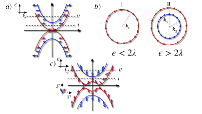
Figure 1: (a-b) Energy dispersion of the Dirac-Rashba model and corresponding equilibrium spin texture in $C_{\textrm{6v}}$-symmetric heterostructures (where $\lambda_{\textrm{sv}}=0$). The spin-splitting of the Dirac bands leads to a spin gap of width $2\lambda$, which separates a 2D electron gas-like region of BR-split bands with counter-rotating spin textures (regime II: $\epsilon>2\lambda$) from a spin-helical regime (regime I: $\epsilon<2\lambda$). (c) Same as (a) for graphene heterostructures with $C_{3v}$ point group symmetry. The competition of BR and spin-valley SOC gives rise to a “Mexican hat-shaped” dispersion with an electron/hole pocket at very low energies. Energies are defined with respect to the Dirac point. For visualisation purposes, the bands are plotted along $k_{x}$ with $k_{y}=0$ (i.e. spins lie only in the $yz$ plane).

The low-energy excitations in graphene/TMD bilayers are governed by the following generalized Dirac-Rashba model (we use natural units $\hbar=1$ throughout)

$$H_{\xi}=\intop d\mathbf{x}\,\Psi_{\xi}^{\dagger}\left[-\imath\mathit{v}\,\boldsymbol{\sigma}\cdot\mathbf{\boldsymbol{\nabla}}+V_{\mathit{\textrm{SO}}}^{\xi}+U\left(\mathbf{x}\right)\right]\Psi_{\xi}\,,$$ (1)

where $\xi=\pm 1$ signs refer to inequivalent valleys $K(+)$ and $K^{\prime}(-)$, $(\Psi_{\xi},\Psi_{\xi}^{\dagger})\equiv(\Psi_{\xi}(\mathbf{x}),\Psi_{\xi}^{\dagger}(\mathbf{x}))$ are 4-component spinor fields defined on the internal spaces of pseudospin and spin and $v$ is the velocity of massless Dirac fermions (here, $\boldsymbol{\sigma}$ is the vector of Pauli matrices acting on the pseudospin space). The term $V_{\mathit{\textrm{SO}}}^{\xi}$ describes the spatially uniform proximity-induced SOC on the graphene layer and comprises several contributions that reflect the $C_{3v}$ point group symmetry of the heterostructure (Wang_2015, ; Fabian_2017, ; Cysne_2018, ). For instance, the breaking of mirror reflection symmetry about the graphene plane allows $z\rightarrow-z$ asymmetric SOC. This so-called BR effect (Bychkov_1984, ) is generically present in graphene on a substrate and is responsible for the entanglement between pseudospin and spin degrees of freedom (Rashba_2009, ), with clear signatures in the spin dynamics (Tuan_2014, ) and current-induced spin-orbit torque (Sousa_2020, ). Moreover, the spin-orbit interactions imprinted on the graphene layer acquire sublattice-resolved terms inherited from the noncentrosymmetric TMD layer, namely the spin-valley coupling, as mentioned in the Introduction. All together, in the longwavelenght limit, $V_{\mathit{\textrm{SO}}}^{\xi}$ generally contains three SOC terms compatible with the $C_{3v}$ point group i.e.,

$$V_{\mathit{\textrm{SO}}}^{\xi}=V_{\textrm{KM}}+V_{\textrm{BR}}+V_{\textrm{sv}}^{\xi},$$ (2)

where $V_{\textrm{KM}}\propto\sigma_{z}s_{z}$ is the intrinsic-type Kane-Mele SOC (KaneMele_2005, ; KaneMele_2005b, ), $V_{\textrm{BR}}\propto(\sigma_{x}s_{y}-\sigma_{y}s_{x})$ describes the BR effect, (Rashba_2009, ) $V_{\textrm{sv}}^{\xi}\propto\xi s_{z}$ captures the spin-valley effect which acts on charge carriers as a valley-Zeeman coupling (Srivastava_2015, ), and $\mathbf{s}$ is the vector of Pauli matrices acting on the spin space. In practice, the weak $z\rightarrow-z$ symmetric Kane-Mele SOC can be neglected in comparison to the other effects (see, for example, Ref. (Gmitra_2016, )) and hence in this work, we approximate the spin-orbit interaction as follows

$$V_{\mathit{\textrm{SO}}}^{\xi}\simeq\lambda\left(\boldsymbol{\sigma}\times\mathbf{s}\right)_{z}+\xi\lambda_{\textrm{sv}}s_{z}.$$ (3)

Beyond SOC, the proximity coupling to a TMD also imprints a sublattice-staggered potential $H_{\Delta}^{\xi}=\Delta\xi\sigma_{z}$ on the graphene sheet. The staggered on-site energy is believed to be substantially smaller than the SOC energy scales in Eq. (3) (under 0.1 meV according to a recent study (Pezo_2020, )) and because it plays a very limited role in both the spin dynamics (Offidani_2018, ) and coupled spin-charge transport effects (Offidani_2017, ), we neglect it in the following discussion. We note that more SOC terms are allowed if additional crystal symmetries are broken further reducing the point group of the heterointerface. These include unconventional in-plane-polarized spin-valley and Kane-Mele-type SOC that are symmetry-allowed in graphene coupled to low-symmetry TMDs (Cysne_2018, ), the implications of which are beyond the scope of the present work. Finally, the last term in Eq.(1) is a random potential produced by scalar impurities, which will be responsible for the extrinsic generation of nonequilibrium spin polarization and spin Hall currents to be discussed in Secs. IV-VI.

The energy-momentum dispersion relation of the low-energy Dirac bands reads as

$$\epsilon_{ln}\left(\mathbf{k}\right)=l\sqrt{v^{2}k^{2}+[M_{n}(k)]^{2}},$$ (4)

where $M_{n}(k)=[2\lambda^{2}+\lambda_{\textrm{sv}}^{2}+2n\sqrt{\lambda^{4}+(\lambda^{2}+\lambda_{\textrm{sv}}^{2})v^{2}k^{2}}]^{1/2}$ is the spin gap induced by SOC, $n,l=\pm 1$ are the band indices and $k=|\mathbf{k}|$ (with $\mathbf{k}$ measured from a $K$ point). Equation (4) makes manifest the underlying particle-hole symmetry of the Hamiltonian, which results in one or two Dirac bands at the Fermi energy $\varepsilon$ depending on the gate-tunable charge carrier density (see Fig. 1). To ease the notation, we shall assume $\epsilon,\lambda_{\textrm{sv}},\lambda>0$ in what follows. Inverting Eq.(4) and evaluating the energy-momentum dispersion relation at the Fermi energy $\epsilon_{ln}=\varepsilon$, one obtains the Fermi momenta, $k_{ln}=k(\epsilon_{ln}=\varepsilon)$, as follows

$$k_{ln}=v^{-1}\sqrt{\lambda_{\textrm{sv}}^{2}+\varepsilon^{2}\pm 2\sqrt{\lambda^{2}\varepsilon^{2}+\lambda_{\textrm{sv}}^{2}\varepsilon^{2}-\lambda^{2}\lambda_{\textrm{sv}}^{2}}}.$$ (5)

The $\pm$ sign depends on the energy range within which lies the Fermi energy $\varepsilon$ (Fig. 1). The eigenvectors, $\psi_{ln}(\mathbf{x})=e^{i\mathbf{k}\cdot\mathbf{x}}\Phi_{ln}(\mathbf{k})$, have the following spinorial structure

$$\Phi(k_{ln},\theta)=\left(\begin{array}[]{c}e^{-i\theta}\\ i\alpha\\ \beta\\ i\gamma e^{i\theta}\end{array}\right)$$ (6)

with $\theta$ the momentum angle with respect to an arbitrary axis in the graphene plane and $\alpha,\beta$ and $\gamma$ given by

$$\alpha = \frac{(\epsilon_{ln}-\lambda_{\textrm{sv}})^{2}-v^{2}k_{ln}^{2}}{2\lambda vk_{ln}},$$ (7)

$$\beta = \frac{\epsilon_{ln}-\lambda_{\textrm{sv}}}{vk_{ln}},$$ (8)

$$\gamma = \frac{(\epsilon_{ln}-\lambda_{\textrm{sv}})^{2}-v^{2}k_{ln}^{2}}{2\lambda(\epsilon_{ln}+\lambda_{\textrm{sv}})}.$$ (9)

In this work we specialize to the regime I which should be experimentally accessible in ultra-clean devices with strong interfacial SOC. The Fermi energy therefore lies in the interval $\varepsilon_{-}\equiv\lambda_{sv}<\varepsilon<\sqrt{4\lambda^{2}+\lambda_{sv}^{2}}\equiv\varepsilon_{+}$ [Fig. 1 (c)], which we call spin-helical regime, where the simply-connected Fermi surface topology is akin to ideal topological surface states (Schwab_2011, ). For that reason, we will drop the band indices and define the Fermi momentum in regime I as $k_{F}\equiv k_{1,-1}$ with $k_{1,-1}=k_{1,-1}(\varepsilon)$ as per Eq.(5).

For the transport calculations below, we will also need the density of states at the Fermi level, per valley,

$$N_{F}=\frac{\varepsilon(\lambda^{2}+\lambda_{\textrm{sv}}^{2}+\sqrt{\lambda^{2}\varepsilon^{2}+\lambda_{\textrm{sv}}^{2}(\varepsilon^{2}-\lambda^{2})})}{2\pi v^{2}\sqrt{\varepsilon^{2}(\lambda^{2}+\lambda_{\textrm{sv}}^{2})-\lambda^{2}\lambda_{\textrm{sv}}^{2}}}.$$ (10)

From this expression, one easily recovers pristine graphene’s well-known expression $N_{0}=\varepsilon/(2\pi v^{2})$ by letting $\lambda_{\textrm{sv}}\rightarrow 0$ first and then $\lambda\rightarrow 0$. We will show below that in this regime, where the electronic states have a well-defined spin helicity, the pseudospin and spin degrees of freedom are constrained in such a way that it becomes possible a full description of the coupled spin-charge dynamics in terms of a single transport equation.

III The Keldysh technique

The Keldysh formalism, which goes back to the pioneering works by Schwinger (Schwinger_1961, ) and Keldysh (Keldysh_1965, ), is a powerful generalization of the standard perturbative approach of equilibrium quantum field theory to nonequilibrium problems. Within the Keldysh technique (Kadanoff_1962, ; Raimondi_2003, ; Rammer_2007, ; Kamenev_2009, ; Raimondi_2016, ), the Green’s function has the following matrix structure

$$\check{G}=\left(\begin{array}[]{cc}G^{R}&G^{K}\\ 0&G^{A}\end{array}\right),$$ (11)

with $G^{R},G^{A}$ and $G^{K}$ the respective retarded, advanced and Keldysh components. The Green’s function acts on the spin, valley and pseudospin spaces, and thus each block in Eq. (11) can be represented as a $8\times 8$ matrix. $\check{G}$ satisfies the left-right subtracted Dyson equation (Rammer_1986, ), which conveniently gets rid of the delta-function singularity at coinciding space-time points, i.e.

$$\left[\left(\check{G_{0}}\right)^{-1},\check{G}\right]=\left[\check{\Sigma},\check{G}\right],$$ (12)

where the square brackets define the commutator. Here the products are to be understood with respect to both the Keldysh and internal spin spaces and to the space-time coordinates (i.e. convolution products). The kinetic and proximity-induced SOC terms are contained in the bare Green’s function $\check{G_{0}}$, whereas the quasiparticle self-energy $\check{\Sigma}$ is due to the disorder potential. In the following the self-energy will be obtained by averaging, term by term, the perturbative expansion of the left-right subtracted Dyson equation in the potential $U\left(\mathbf{x}\right)$ with respect to the disorder configuration. The Green’s function $\check{G}$ entering Eq.(12) is then the disorder-averaged Green’s function. In explicit terms, we have

$$\left(\check{G}_{0}\left(X_{1};X_{2}\right)\right)^{-1}=\left(i\partial_{t_{1}}-h\left(\mathbf{x_{1}}\right)\right)\delta\left(t_{1}-t_{2}\right)\delta\left(\mathbf{x_{1}-\mathbf{x_{2}}}\right)\,,$$

with $X_{1}\equiv\mathbf{\mathbf{(x_{1}},}t_{1})$, $X_{2}\equiv\mathbf{\mathbf{(x_{2}},}t_{2})$ and $h\left(\mathbf{x}\right)$ the Hamiltonian density as derived from the disorder-free part in Eq. (1). The externally applied (uniform) electric field $\mathbf{E}$ is incorporated by means of the standard minimal coupling within the velocity gauge, $-i\boldsymbol{\nabla}\rightarrow-i\boldsymbol{\nabla}-e\mathbf{E}\,t$ (Rammer_1986, ; Rammer_2007, ), $t$ being the center-of-mass time defined below and $e>0$ the unit of electric charge.

The aim of this work is to derive a coupled spin-charge transport equation in the spin-helical regime. Following the standard approach, we define the center-of-mass and relative space-time coordinates

$$\mathbf{x}=\frac{1}{2}\left(\mathbf{x_{1}+\mathbf{x_{2}}}\right),\quad t=\frac{1}{2}\left(\mathbf{\mathrm{t}_{\mathrm{1}}+\mathrm{t}_{\mathrm{2}}}\right)\,,$$ (13)

$$\mathbf{r}=\mathbf{x}_{1}-\mathbf{x}_{2},\qquad\tau=t_{1}-t_{2}\,.$$ (14)

As customary, we introduce Wigner-mixed coordinates by taking the Fourier transform with respect to the $\mathbf{r}$ and $\tau$ variables. The key assumption in the derivation of the transport equation is that the center-of-mass space-time variable $\mathbf{x},t$ is a slow variable compared to $\mathbf{r},\tau$. As a result one can perform a gradient expansion (see Appendix A for details) of Eq.(12) obtaining for $\check{G}\left(\mathbf{x},t,\mathbf{k},\omega\right)\equiv\check{G}$ the following equation of motion

$$\partial_{t}\check{G}+\frac{1}{2}\left\{\boldsymbol{\sigma\cdot},\left(\nabla-e\mathbf{E\partial_{\omega}}\right)\check{G}\right\}+\qquad$$

$$+i\left[h\left(\mathbf{k}\right),\check{G}\right]-\frac{1}{2}\left\{e\mathbf{E\cdot},\nabla_{\mathbf{k}}\check{G}\right\}=-i\left[\check{\Sigma},\check{G}\right],$$ (15)

where $h\left(\mathbf{k}\right)$ is the Fourier-transformed bare Hamiltonian density and the curly brackets denote, as usual, the anticommutator. In a compact form, Eq. (15) provides the equation of motion for all the components of the Green’s function Eq.(11). The Keldysh component in the right hand side term of Eq.(15) is usually named collision integral and, in the spirit of the semiclassical Boltzmann transport theory, it can be divided in a $in$- and $out$-term according to

$$I =-i\left(\Sigma^{R}G^{K}-G^{K}\Sigma^{A}\right)+$$

$$+i\left(G^{R}\Sigma^{K}-\Sigma^{K}G^{A}\right)\equiv I_{out}+I_{in}\,.$$ (16)

The retarded and advanced clean Green’s functions are given by

$$G_{0\mathbf{k}}^{R,A}=\sum_{l,n}\frac{P_{ln}\left(\mathbf{k}\right)}{\omega-\epsilon_{ln}\left(\mathbf{k}\right)\pm i0^{+}},$$ (17)

where $P_{ln}\left(\mathbf{k}\right)=|\Phi(k_{ln},\theta)\rangle\langle\Phi(k_{ln},\theta)|$ is the projector onto the eigenstate with indices $ln$. In the spin-helical regime only the projector $P_{1-1}\left(\mathbf{k}\right)\equiv P\left(\mathbf{k}\right)$ is relevant and we omit the band indices hereafter for simplicity.

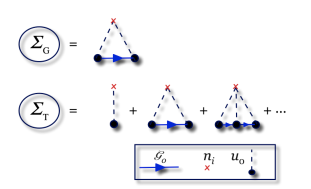
Figure 2: Disorder self energy in the non-crossing approximation. In the Gaussian case, the self energy consists of a single “rainbow” diagram with two potential insertions ($\Sigma_{G}$). In the $T$-matrix approach, one effectively resums the full series of single-impurity scattering events ($\Sigma_{T}$), which is then proportional to the impurity areal density $n_{i}$.

In the presence of random impurities with areal density $n_{i}$, the retarded and advanced Green’s functions are dressed with the corresponding disorder self-energies. The self energy is given by the average over disorder ($\prec...\succ$) of the $T$-matrix expansion as shown in Fig. 2, that is,

$$\Sigma^{R(A)}=T^{R(A)}=n_{i}\frac{u_{0}^{2}\mathcal{G}^{R(A)}}{1-u_{0}\mathcal{G}^{R(A)}}.$$ (18)

In the above $\mathcal{G}^{R(A)}=G_{0}^{R(A)}(\mathbf{x},\mathbf{x})$ is the local retarded (advanced) clean Green’s function, i.e. evaluated at coinciding space arguments and the disorder average is defined by

$$\prec U\left(\mathbf{x}\right)\succ = u_{0}\,,$$

$$\prec U\left(\mathbf{x}\right)U\left(\mathbf{x^{\prime}}\right)\succ = u_{0}^{2}\delta\left(\mathbf{x}-\mathbf{x}^{\prime}\right)\,,$$

$$\prec U\left(\mathbf{x}\right)U\left(\mathbf{x}^{\prime}\right)U\left(\mathbf{x}^{\prime\prime}\right)\succ = u_{0}^{3}\delta\left(\mathbf{x}-\mathbf{x}^{\prime}\right)\delta\left(\mathbf{x}^{\prime}-\mathbf{x}^{\prime\prime}\right)\,,$$

and so on and so forth.

In the equation of motion, one determines the Green function self-consistently by replacing $\mathcal{G}^{R(A)}$ with the disorder-average one $G^{R(A)}$. To quadratic order in the disorder potential, in the so-called first Born approximation, one keeps only the first term of the series expansion of Eq. (18). The corresponding retarded/advanced self-energies read as

$$\Sigma^{R(A)}=n_{i}u_{0}^{2}\int\frac{d\mathbf{k^{\prime}}}{(2\pi)^{2}}G_{0\mathbf{k^{\prime}}}^{R,A}=\mp i\pi n_{i}u_{0}^{2}N_{F}\left\langle P\left(\mathbf{k}_{F}\right)\right\rangle,$$ (19)

where from now $\left\langle\ldots\right\rangle$ indicates the integration, normalized to $2\pi$, over the wavevector angle defining the direction of $\mathbf{k}_{F}$. As a result the $out-$contribution of the collision integral becomes

$$I_{out}=-i\left(T^{R}G^{K}-G^{K}T^{A}\right).$$ (20)

In a self-consistent evaluation of the self-energy, one should replace $G_{0\mathbf{k}}^{R,A}$ with the disorder-averaged Green’s function $G_{\mathbf{k}}^{R,A}$ in Eq.(19). Provided one is not too close to the Dirac point, one can neglect the disorder correction to the electron spectrum and the self-consistent solution for the self-energy is reasonably approximated by the expression in Eq.(19).

Next, we consider the Keldysh self-energy, which determines the $in$-contribution of the collision integral. The perturbation expansion of the Keldysh Green’s function reads quite different from that of the retarded and advanced Green’s functions. After disorder averaging, at each order in $u_{0}$, there are as many terms as positions in which the Keldysh component can be placed with the additional requirement that on the left (right) of the Keldysh component there can be only retarded (advanced) Green’s functions. For instance, at first and second orders one has

$$G^{K\left(1\right)} =G_{0}^{R}u_{0}G_{0}^{K}+G_{0}^{K}u_{0}G_{0}^{A},$$

$$G^{K\left(2\right)} =G_{0}^{R}u_{0}\left(G_{0}^{R}u_{0}G_{0}^{K}+G_{0}^{K}u_{0}G_{0}^{A}\right)+G_{0}^{K}u_{0}G_{0}^{A}u_{0}G_{0}^{A}\,.$$

In the end, the Keldysh self-energy then reads

$$\Sigma^{K}=n_{i}u_{0}^{2}\overline{T}^{R}\int\frac{d\mathbf{k}^{\prime}}{\left(2\pi\right)^{2}}G_{\mathbf{k}^{\prime}}^{K}\overline{T}^{A},$$ (21)

where we have introduced the following notation

$$T^{R(A)}=n_{i}u_{0}^{2}G^{R\left(A\right)}\overline{T}^{R(A)}$$ (22)

with

$$\overline{T}^{R(A)}=\frac{1}{1-u_{0}G^{R(A)}}.$$ (23)

Interestingly, only the $\overline{T}^{R,A}$ parts of the $T$-matrices appear in the Keldysh self-energy upon performing the disorder average as a result of the latter involving impurity insertions in both the retarded and advanced Green’s functions at the left and right of the Keldysh Green’s function, respectively. This corresponds to the so-called $T$-matrix insertion in the vertex correction of the Kubo linear response formalism, which effectively resums the infinite set of single-impurity scattering diagrams (Milletari_2016a, ; Milletari_2016b, ). The ”in” contribution to the collision integral Eq.(16) finally reads

$$I_{in}=in_{i}u_{0}^{2}\int\frac{d\mathbf{k}^{\prime}}{\left(2\pi\right)^{2}}\left(G_{\mathbf{k}}^{R}\overline{T}^{R}G_{\mathbf{k}^{\prime}}^{K}\overline{T}^{A}-\overline{T}^{R}G_{\mathbf{k}^{\prime}}^{K}\overline{T}^{A}G_{\mathbf{k}}^{A}\right).$$ (24)

After some algebra, it is possible to recast the collision integral Eq.(16) in the form (for details see Appendix B)

$$I=I_{in}+I_{out}=in_{i}u_{0}^{2}\int\frac{d^{2}\mathbf{k^{\prime}}}{(2\pi)^{2}}\Big{(}G_{\mathbf{k}}^{R}\overline{T}^{R}G_{\mathbf{k^{\prime}}}^{K}\overline{T}^{A}-\overline{T}^{R}G_{\mathbf{k^{\prime}}}^{K}\overline{T}^{A}G_{\mathbf{k}}^{A}-G_{\mathbf{k^{\prime}}}^{R}\overline{T}^{R}G_{\mathbf{k}}^{K}\overline{T}^{A}+\overline{T}^{R}G_{\mathbf{k}}^{K}\overline{T}^{A}G_{\mathbf{k^{\prime}}}^{A}\Big{)}.$$ (25)

From the point of view of the kinetic equation, the variables $\mathbf{k}$ and $\mathbf{k^{\prime}}$ represent the momentum before and after a single-impurity scattering event, depending whether one considers the $in$- and $out$-contributions. One can easily check that the detailed balance is satisfied. If $\mathbf{k}\leftrightarrow\mathbf{k^{\prime}}$, the $in-$ and $out-$terms are interchanged and then the microscopic reversibility of the scattering probability is preserved (Lebowitz_1995, ). The general expression Eq.(25) is one of the main results of this work. The familiar case of a Fermi gas with Gaussian white-noise correlation is recovered by letting $\overline{T}^{R(A)}\rightarrow 1$.

IV The Eilenberger equation

In this section, we solve the kinetic equation presented earlier (cf. Eq.(15) and the following discussion) within the quasiclassical approximation (Rammer_1986, ; Rammer_2007, ; Raimondi_2003, ). The latter has a resemblance to the standard Boltzmann transport theory that lends itself to a physically transparent interpretation of 2D spin-orbit coupled transport effects in the experimentally relevant diffusive regime (Offidani_2018c, ; Milletari_2016a, ; Sousa_2020, ).

The established framework in which the quasiclassical theory is expressed is that of the real-time formulation of the Keldysh technique, as discussed above. The quasiclassical Green’s function $\check{g}$ is usually defined by (Eilenberger_1968, )

$$\check{g}\left(\mathbf{x},t,\mathbf{n},\omega\right)\doteq\frac{i}{\pi}\intop_{\mathcal{C}}d\xi\,\check{G}\left(\mathbf{x},t,\mathbf{k},\omega\right)$$ (26)

where we have introduced the variable $\xi=\epsilon_{1-1}(k)-\varepsilon$ in terms of the dispersion relation of the spin-helical band at the Fermi energy. Since we assumed $\varepsilon>0$, all the projectors in what follows are constructed from eigenstates $l=1,n=-1$. The integration contour $\mathcal{C}$ is taken in such a way to capture the contribution of the Green’s function pole, and that the $\xi$-integration leaves unaffected the angular dependence described by the unit vector $\mathbf{n}=\mathbf{k}/\left|\mathbf{k}\right|$. The so-called Eilenberger equation is then obtained by applying the $\xi$-integration to the Eq.(15) by reasonably assuming that the self-energy does not have a further singular behavior, which would add to the Green’s function pole. At the leading order in the weak-disorder expansion $\varepsilon\tau\gg 1$, with $\tau=1/(2\textrm{Im}\,\Sigma^{A})$ the quasiparticle lifetime, the $\xi$-integration procedure is not affected by the disorder-induced dressing of the pole. The Eilenberger equation then reads

$$\partial_{t}\check{g}+\frac{1}{2}\left\{\boldsymbol{\sigma\cdot},\left(\boldsymbol{\nabla}-e\mathbf{E\partial_{\omega}}\right)\check{g}\right\}+\qquad\quad$$

$$+i\left[h\left(\mathbf{\mathbf{k}_{F}}\right),\check{g}\right]=-i\left[\check{\Sigma},\check{g}\right].$$ (27)

The quasiclassical Green’s function has the same triangular matrix structure of the original Green’s function, i.e.

$$\check{g}=\left(\begin{array}[]{cc}g^{R}&g\\ 0&g^{A}\end{array}\right),$$ (28)

and in the clean system, the retarded (advanced) quasiclassical Green’s function are

$$g^{R(A)}=\pm P(\mathbf{k}_{F})\equiv\pm P\left(\theta\right),$$ (29)

where $P(\mathbf{k}_{F})\equiv P\left(\theta\right)$ is the projector on the spin-helical band evaluated at the Fermi energy with only the angle dependence remaining. In principle, we have to solve Eq. (27) for all the components of $\check{g}$, but one can considerably simplify the problem by noting that the elastic scattering from scalar impurities merely produces a shift in the pole of the retarded (advanced) component. Hence, as already mentioned, the expression (29) remains unchanged at leading order in powers of $\left(\varepsilon\tau\right)^{-1}$. Ultimately $g^{R(A)}$ gives information about the density of states whereas $g^{K}\equiv g$ provides the distribution function. Finally, the Eilenberger equation for the Keldysh component Eq. (27) becomes

$$\partial_{t}g+\frac{1}{2}\left\{\boldsymbol{\sigma\cdot},\left(\nabla-e\mathbf{E\partial_{\omega}}\right)g\right\}+i\left[h\left(\mathbf{k_{F}}\right),g\right]=\mathcal{I},$$ (30)

where the $\xi$-integration must be performed also in the right hand side of Eq. (15). Explicitly, by applying the $\xi$-integration to the expression of $I$ given by Eq. (25) and anticipating the definition of the scattering time given below in the Eq. (32), we obtain

$$\mathcal{I}=-\frac{1}{2\tau_{0}}\left(\left\langle g^{R}\right\rangle\overline{T}^{R}g\overline{T}^{A}-\overline{T}^{R}g\overline{T}^{A}\left\langle g^{A}\right\rangle\right)+$$ (31)

$$+\frac{1}{2\tau_{0}}\left(g^{R}\overline{T}^{R}\left\langle g\right\rangle\overline{T}^{A}-\overline{T}^{R}\left\langle g\right\rangle\overline{T}^{A}g^{A}\right),$$

where, for brevity, we defined $g^{R;A;K}\equiv g^{R,A,K}\left(\theta,\omega\right)$ and its angle averaged $\left\langle g^{R,A,K}\right\rangle=\left\langle g^{R,A;K}\left(\theta^{\prime},\omega\right)\right\rangle$ with $\theta$ and $\theta^{\prime}$ the angles of $\mathbf{k}$ and $\mathbf{k^{\prime}}$, respectively, both momenta evaluated at the Fermi surface. For convenience we have also introduced the basic scattering rate

$${\color[rgb]{0,0,0}1/\tau_{0}=2\pi N_{0}n_{i}u_{0}^{2}\,,}$$ (32)

which has the meaning of the inverse quasiparticle lifetime of graphene without the SOC in the Gaussian limit.

By looking at Eq. (30) we note two key differences with respect to the semiclassical Boltzmann transport equation (BTE): (1) there is a commutator term $i\left[h\left(\mathbf{k_{F}}\right),g\right]$ missing in the BTEs because there $g$ is a scalar, (2) a general scattering kernel is present which, in principle, holds for any type of impurity (magnetic, etc.), whereas semiclassical BTEs based on a scalar distribution function only applies to scalar impurities. Although not considered in the present paper, the method can be readily extended to impurity potential with a matrix structure in the internal degrees of freedom.

In the remainder of this paper, we confine our analysis to the case of a constant and uniform electric field for which the space and time derivatives in the Eq. (30) drop out and the quasiclassical Green’s function then depends only on $\mathbf{n},\omega$ or equivalently on $\theta,\omega$. To leading order in $\mathbf{E}$, one can safely replace $g$ in the force term (in the left hand side) by the equilibrium Keldysh Green’s function. The Eilenberger equation (30) then reduces to

$$-\frac{1}{2}\left\{\boldsymbol{\sigma\cdot},e\mathbf{E\partial_{\omega}}g_{eq}(\theta,\omega)\right\}+i\left[h\left(\mathbf{k_{F}}\right),g\right]=\mathcal{I},$$ (33)

where $g_{eq}(\theta,\omega)=f(\omega)P(\theta)$ is the equilibrium quasiclassical Keldysh Green’s function with

$$f(\omega)=2\tanh\left(\frac{\omega}{2T}\right),$$ (34)

where $T$ is the temperature (in our natutal units $k_{B}=1$).

To proceed further, following Ref. (Schwab_2011, ), we propose the following ansatz for the quasiclassical Keldysh Green’s function

$$g(\theta,\omega)=g_{0}(\theta,\omega)\,P(\theta)\,,$$ (35)

where $g_{0}\left(\theta,\omega\right)$ is a scalar function. Although $g$ is still a matrix, its structure is entirely constrained. The ansatz can be motivated by the following argument. Inspection of the Eq.(30) shows that, at leading order in the dilute regime ($\varepsilon\tau\gg 1$), the solution must commute with the Hamiltonian and be of order $g\sim\tau\sim\tau_{0}$. The commutator in the left hand side, although of order $\varepsilon\tau\gg 1$, vanishes because the Hamiltonian density at the Fermi level can be written as $h\left(\mathbf{k_{F}}\right)=\varepsilon P(\theta)$ and the remaining terms in the equation are of order unity. We note that this ansatz may not be sufficient when one is dealing with quantum (weak-localization) corrections in the weak-disorder expansion. Using these ingredients and by taking the trace of the Eq.(31) one gets a scalar collision integral for $g_{0}$

$$\mathcal{I}_{0}=-\int_{0}^{2\pi}\frac{\mathrm{d\theta^{\prime}}}{2\pi}W\left(\vartheta\right)\left[g_{0}\left(\theta,\omega\right)-g_{0}\left(\theta^{\prime},\omega\right)\right],$$ (36)

where

$$W\left(\vartheta\right)=\frac{N_{F}}{N_{0}}\frac{1}{\tau_{0}}\mathrm{Tr}\left[P(\theta)\overline{T}^{R}P(\theta^{\prime})\overline{T}^{A}\right]$$ (37)

is a function of the angle difference that from now we call $\vartheta\equiv\theta-\theta^{\prime}$.

In the end, once the solution for the quasiclassical Green’s function $g_{0}(\theta,\omega)$ is known one can easily obtain the steady-state observables, such as the electric current, the spin polarization and the spin current densities. According with the general recipe in the Abelian case (Konschelle_2014, ; Kadanoff_1962, ), using the notation (Rammer_1986, )

$$\intop\frac{d\mathbf{k}}{(2\pi)^{2}}\int\frac{d\omega}{2\pi i}\approx N_{F}\int\frac{d\mathbf{n}}{2\pi}\int\frac{d\omega}{2\pi i}\int d\xi,$$ (38)

if $O=\sigma_{i}\otimes s_{j}$ indicates a generic observable, its quantum statistical non-equilibrium average $\mathcal{O}$ is given by

$$\mathcal{O} \equiv \frac{i}{2}\intop\frac{d\omega}{2\pi}\intop\frac{d\mathbf{k}}{(2\pi)^{2}}\>\mathrm{Tr}\left[OG^{K}\left(\mathbf{k},\omega\right)\right]$$ (39)

$$= -\frac{N_{F}}{4}\intop d\omega\langle Tr\,\left[Og\left(\theta,\omega\right)\right]\rangle$$

$$= -\frac{N_{F}}{4}\intop d\omega\langle g_{0}\left(\theta,\omega\right)Tr\,\left[OP\left(\theta\right)\right]\rangle,$$

$$= -\frac{N_{F}}{2}\intop d\omega\langle g_{0}\left(\theta,\omega\right)O_{{\bf k}}\rangle,$$

where $O_{\mathbf{k}}=\textrm{Tr}\left[O\,P(\theta)\right]/2$ indicates the equilibrium average and, as before, $\left\langle\ldots\right\rangle$ is the integration over the directions of $\mathbf{k}=k_{F}\mathbf{n}$. The trace symbol involves all internal degrees of freedom: sublattice, valley and spin. Because intervalley scattering is neglected for simplicity (the impurity potential $U(\mathbf{x})$ is a scalar quantity), the trace over the valley degree of freedom yields a simple factor of two, which is compensated by the factor of two in the denominator in the definition of the equilibrium average of $O_{\mathbf{k}}$. The relevant observables are the charge current ($\mathbf{J}=-ev\boldsymbol{\mathbf{\sigma}}\otimes s_{0}$), spin polarization ($\mathbf{S}=\frac{\hbar}{2}\sigma_{0}\otimes\mathbf{s}$) and z-polarized spin Hall current ($\mathbf{J}_{s}^{z}=\frac{\hbar v}{2}\boldsymbol{\sigma}\otimes s_{z}$). Here we have reinstated the Planck constant for the sake of clarity. For the $C_{3v}$-invariant model with spin-valley coupling, the equilibrium charge current, spin polarization density and (persistent) spin Hall current can be easily evaluated as

$$\mathbf{J}_{\mathbf{k}}=(-ev)\frac{2(\beta+\alpha\gamma)}{1+\alpha^{2}+\beta^{2}+\gamma^{2}}\mathbf{n}\,,$$ (40)

$$\mathbf{S}_{\mathbf{k}}=\hbar\frac{(\alpha+\beta\gamma)}{1+\alpha^{2}+\beta^{2}+\gamma^{2}}\hat{z}\times\mathbf{n}\,,$$ (41)

$$\mathbf{J}_{s\mathbf{k}}^{z}=(\hbar v)\frac{(\beta-\alpha\gamma)}{1+\alpha^{2}+\beta^{2}+\gamma^{2}}\mathbf{n}\,,$$ (42)

where $\alpha,\beta$ and $\gamma$ depend on the parameters of the Hamiltonian and on the Fermi energy as defined in the Eq.(6).

Similar to the well-studied high density regime with two occupied Dirac bands (Milletari_2017, ; Offidani_2017, ; Offidani_2018b, ; Sousa_2020, ), the standard first Born approximation will allows us to obtain the leading semiclassical contribution to the nonequilibrium spin polarization density generated by the inverse spin galvanic effect, namely $\mathcal{S}_{i}\propto\epsilon_{ij}\epsilon\tau\,E_{j}$, with $\epsilon_{ij}$ the Levi-Civita symbol and $i,j=x,y$. On the other hand, the calculation of the steady-state $\hat{z}$-polarized spin Hall current density, $\mathcal{J}_{i}^{z}\propto\epsilon_{ij}\epsilon\tau\,E_{j}$, will require higher-order corrections to the self-energy due to the pivotal role played by skew scattering mechanism in the extrinsic spin Hall effect.

V The Eilenberger equation in the First Born approximation

In this section we consider the self-consistent Born approximation, which amounts to confine to second order in the disorder potential expansion, implying $\overline{T}^{R(A)}\longrightarrow 1$. As a result, the matrix transport equation (33) reduces to a simpler scalar effective transport equation for the “charge” component $g_{0}\left(\theta,\omega\right)$ of the quasiclassical Green’s function

$$\left(\mathbf{E}\cdot\mathbf{J}_{{\bf k}}\right)\partial_{\omega}f=-\frac{1}{2\pi}\intop_{0}^{2\pi}d\theta^{\prime}\,W\left(\vartheta\right)\left(g_{0}\left(\theta,\omega\right)-g_{0}\left(\theta^{\prime},\omega\right)\right),$$ (43)

where

$$W\left(\vartheta\right)=\frac{N_{F}}{N_{0}}\frac{1}{\tau_{0}}\mathrm{Tr}\{P\left(\theta\right),P\left(\theta^{\prime}\right)\}.$$ (44)

is the scattering kernel in the first Born approximation [c.f. Eq. (37)]. We remind the reader that, unless otherwise stated, the projectors are evaluated at the Fermi surface. Due to the periodicity of the projectors, the scattering kernel can only depend on the difference of the two angles. Furthermore due to the cyclic property of the trace, the expression is invariant under the interchange of the two angles, implying that the effective kernel is an even periodic function of the angle difference $\vartheta\equiv\theta-\theta^{\prime}$. The transport equation Eq.(43) together with the expressions of the effective kernel Eq.(44) and the velocity vertex Eq.(40), defines the coupled spin-charge response of the projected band at the Fermi energy. This is one of the central results of this paper and can be used to obtain the charge conductivity and spin-galvanic conductivity of the spin-helical band as discussed below.

We first illustrate the formalism with the $C_{6v}$-invariant Dirac-Rashba model obtained by setting $\lambda_{\textrm{sv}}=0$ in Eq. (3); the corresponding band structure and spin texture is shown in Fig. 1(a). In this case, the eigenvalue coefficients are $\alpha=-\beta=-\varepsilon/\sqrt{\varepsilon(\varepsilon+2\lambda)}$, $\gamma=-1$ and one can obtain simple analytical expressions for all the transport coefficients. In particular the equilibrium averages (40-42) read as

$${\bf J}_{{\bf k}} = (-ev)\frac{\sqrt{\varepsilon(\varepsilon+2\lambda)}}{\varepsilon+\lambda}{\bf n}$$ (45)

$${\bf S}_{{\bf k}} = -\hbar\frac{1}{2}\frac{\sqrt{\varepsilon(\varepsilon+2\lambda)}}{\varepsilon+\lambda}{\hat{{\bf z}}}\times{\bf n}$$ (46)

$$\mathbf{J}_{s\mathbf{k}}^{z} = 0.$$ (47)

The scattering kernel within the first Born approximation reads as (see Appendix C for details)

$$W(\vartheta)=\frac{1}{\tau_{0}}\frac{((2\lambda+\varepsilon)\cos(\theta-\theta^{\prime})+\varepsilon)^{2}}{\varepsilon(\lambda+\varepsilon)}\,.$$ (48)

One sees that the scattering kernel is left-right symmetric ($W(\vartheta)=W(-\vartheta)$) to all orders in the scattering potential, i.e. skew-scattering is absent and no extrinsic spin Hall effect (SHE) can be expected in this case. Interestingly, the absence of any form of SHE is an exact property of the model provided that the impurities are non-magnetic. This is a consequence of the in-plane spin texture of the minimal 2D Dirac-Rashba model and can also be understood from the exact Ward identities for the 4-point vertex function (Milletari_2017, ).

The solution of the transport equation (43) reads

$$g_{0}(\theta,\omega)=-(\partial_{\omega}f)\,\tau_{s}\,{\bf J}_{{\bf k}}\cdot{\bf E},$$ (49)

where

$$\frac{1}{\tau_{s}} = \frac{1}{2\pi}\int_{0}^{2\pi}{\rm d}\theta W(\theta)(1-\cos(\theta))$$ (50)

$$= \frac{1}{2\tau_{0}}\frac{\varepsilon^{2}+4\lambda^{2}}{\varepsilon(\varepsilon+\lambda)}.$$

By using the explicit expressions of the transport time (50) and of the equilibrium average (45) one obtains

$$g_{0}(\theta,\omega)=(ev)(2\tau_{0})(\partial_{\omega}f)\frac{\varepsilon\sqrt{\varepsilon(2\lambda+\varepsilon)}}{4\lambda^{2}+\varepsilon^{2}}\,\mathbf{E}\cdot\mathbf{n},$$ (51)

By inserting this last result in the Eq.(39) and considering the equilibrium average (46) one gets the following current-induced spin polarization

$$\boldsymbol{\mathcal{S}}=\frac{ev\tau_{0}}{\pi v^{2}}\frac{\varepsilon^{2}(\varepsilon+2\lambda)}{(\varepsilon^{2}+4\lambda^{2})}\hat{\mathbf{z}}\times\mathbf{E},$$ (52)

while the charge current reads

$$\boldsymbol{\mathcal{J}}=\frac{2e^{2}\tau_{0}}{\pi\hbar}\frac{\varepsilon^{2}(2\lambda+\varepsilon)}{(4\lambda^{2}+\varepsilon^{2})}\mathbf{E}\,.$$ (53)

These relations imply

$$\boldsymbol{\mathcal{S}}=\frac{\hbar}{2ev}\,\hat{\mathbf{z}}\times\boldsymbol{\mathcal{J}}\,.$$ (54)

The current-induced spin polarization is in plane and orthogonal to the applied electric field as a consequence of the symmetries of the model. In fact, it is easy to see that the inversion symmetry in the plane of graphene implies $\mathcal{S}_{z}=0$ and $\boldsymbol{\mathcal{S}}\cdot\mathbf{E}=0$. This is also the case in the presence of sublattice-staggered interactions (i.e. $\{\lambda_{\textrm{sv}},\Delta\}\neq 0$) due to the existence of a mirror reflection symmetry in the plane of the heterostructure (Sousa_2020, ). The locking of non-equilibrium spin polarization density and charge current in plane at 90 degrees Eq. (54) is thus a general property of non-magnetic graphene heterostructures with $C_{6v}$ or $C_{3v}$ point group symmetry. These restrictions are lifted in magnetic graphene heterostructures, where $\boldsymbol{\mathcal{S}}$ acquires collinear and out of plane components (Sousa_2020, ). We note that Eqs.(52)-(53) coincide exactly with the results for the electric-field-induced spin polarization (Edelstein_1990, ) obtained via the Kubo-Streda linear response theory by Offidani et al (Offidani_2017, ) and confirm the equivalence of the two approaches.

VI The Skew-Scattering mechanism

We now consider the self-energy expansion beyond the first Born approximation. This is relevant for models with non-coplanar spin texture ($\lambda_{\textrm{sv}}\neq 0$ and $\lambda\neq 0$), for which skew scattering mechanism is active and thus the model supports an extrinsic SHE with a semiclassical scaling $J_{i}^{z}\propto\epsilon_{ij}\epsilon\tau E_{j}$, in addition to the intrinsic SHE driven by Berry curvature effects (Offidani_2018c, ; Milletari_2017, ; Garcia_2017, ). The extrinsic mechanism is expected to provide the dominant contribution to the SHE in ultra-clean devices with high charge carrier mobility (i.e. $\epsilon\tau\gg 1$). When the scattering potential is not too strong ($|{\cal G}^{R\left(A\right)}|u_{0}\ll 1$), one may expand the matrices $\overline{T}^{R(A)}$ [c.f. Eqs.(23)] as

$$\overline{T}^{R(A)}\simeq 1+u_{0}\textrm{Re}{\cal G}^{R(A)}\mp iu_{0}\textrm{Im}{\cal G}^{R(A)}.$$ (55)

This approximation corresponds to keeping the first two diagrams in the second line of Fig.  2. We stress that the real part in Eq. (55) does not give contribution to the skew scattering mechanism, but only renormalises the lowest-order scattering amplitude. Mathematically, the skewness in the effective scattering kernel $W(\vartheta)\neq W(-\vartheta)$ results from the imaginary part of the retarded/advanced $T$-matrix, which endows the scattering term in Eq. (43) with an asymmetric contribution,

$$W\left(\vartheta\right)=W(\vartheta)+W_{\textrm{ss}}(\vartheta)$$ (56)

with

$$W_{\textrm{ss}}\left(\vartheta\right)=-ig_{ss}\left(\frac{N_{F}}{N_{0}}\right)^{2}\frac{2}{\tau_{0}}\mathrm{Tr}\left\langle P\left(\theta^{\prime\prime}\right)\right\rangle\left[P\left(\theta\right),P\left(\theta^{\prime}\right)\right]\,,$$ (57)

where the magnitude of the effect is controlled by the “coupling constant”

$$g_{ss}=2\pi u_{0}N_{0}.$$ (58)

The commutator under the trace implies that $W_{\textrm{ss}}$ is odd upon the interchange of $\theta$ and $\theta^{\prime}$ (in particular, $W_{\textrm{ss}}$ vanishes for $\theta=\theta^{\prime}$). A shift $\theta+\psi$, $\theta^{\prime}+\psi$ clearly leaves $W_{\textrm{ss}}$ unchanged because of the periodicity of the projectors with respect to both angles, and hence there can be no dependence on the sum $\theta+\theta^{\prime}$. As a result, $W_{\textrm{ss}}$ must be an odd periodic function of $\vartheta=\theta-\theta^{\prime}$.

The solution of the transport equation generalizes Eq.(49) and reads as

$$g_{0}(\theta,\omega)=-(\partial_{\omega}f)\left(\tau_{\parallel}\mathbf{E}\cdot\mathbf{J}_{\mathbf{k}}+\tau_{\perp}\mathbf{E}\times\mathbf{\mathbf{J}_{\mathbf{k}}}\cdot{\hat{{\bf z}}}\right)\,,$$ (59)

where

$$\tau_{\parallel} =\frac{\tau_{s}}{1+\left(\frac{\tau_{s}}{\tau_{a}}\right)^{2}}\,,\quad\tau_{\perp}=\frac{\tau_{a}}{1+\left(\frac{\tau_{a}}{\tau_{s}}\right)^{2}}\,$$ (60)

are transport times defined through the microscopic rates

$$\tau_{s}^{-1}=\frac{1}{2\pi}\intop_{0}^{2\pi}d\vartheta\,W(\vartheta)(1-\cos(\vartheta))$$ (61)

$$\tau_{a}^{-1}=\frac{1}{2\pi}\intop_{0}^{2\pi}d\vartheta\,W(\vartheta)\sin(\vartheta).$$ (62)

These rates generalize the well-known transport rates in semiclassical transport theory to include the finite asymmetric rates generated by spin-orbit scattering. The expression is formally equivalent to the solution of the linearized Boltzmann transport equations for 2D fermions with SOC (Milletari_2016a, ; Offidani_2018c, ). In Appendix D we derive the expression of the microscopic rates $\tau_{s}^{-1}$ and $\tau_{a}^{-1}$ in terms of the parameters $\alpha$, $\beta$ and $\gamma$ defining the generic eigenvector (6)

$$\frac{\tau}{\tau_{s}} = \frac{2N_{F}}{N_{0}}\frac{\gamma^{4}+1+(\alpha^{2}+\beta^{2})(\alpha^{2}+\beta^{2}-\gamma^{2}-1)}{(1+\alpha^{2}+\beta^{2}+\gamma^{2})^{2}},$$ (63)

$$\frac{\tau}{\tau_{a}} = 2g_{ss}\left(\frac{N_{F}}{N_{0}}\right)^{2}\frac{\left(1-\gamma^{2}\right)\left(\alpha^{2}+\beta^{2}\right)\left(\alpha^{2}+\beta^{2}-\gamma^{2}-1\right)}{(1+\alpha^{2}+\beta^{2}+\gamma^{2})^{3}}.$$ (64)

The zero-temperature nonequilibrium averages to be discussed below are computed according to Eq.(39), taking into account the solution (59). After the integration over $\omega$ one obtains

$$g_{0}\left(\theta\right)\equiv\int_{-\infty}^{\infty}d\omega g_{0}\left(\theta,\omega\right)=-4\left(\tau_{\parallel}\mathbf{E}\cdot\mathbf{J}_{\mathbf{k}}+\tau_{\perp}\mathbf{E}\times\mathbf{\mathbf{J}_{\mathbf{k}}}\cdot{\hat{{\bf z}}}\right)\,.$$ (65)

As a result the nonequilibrium average of a generic observable reads

$$\mathcal{O} = -\frac{N_{F}}{2}\left\langle O_{\mathbf{k}}g_{0}\left(\theta\right)\right\rangle$$ (66)

$$= 2N_{F}\left(\tau_{\parallel}\langle O_{\mathbf{k}}\mathbf{E}\cdot\mathbf{J}_{\mathbf{k}}\rangle+\tau_{\perp}\langle O_{\mathbf{k}}\mathbf{E}\times\mathbf{\mathbf{J}_{\mathbf{k}}}\cdot{\hat{{\bf z}}}\rangle\right).$$

Finally, from the expression Eq.(66) for the physical observables, the Drude conductivity ($\sigma_{xx}=\sigma_{yy}=\mathcal{J}_{x}/E_{x}$), the spin galvanic susceptibility ($\chi_{yx}=-\chi_{xy}=\mathcal{S}_{y}/E_{x}$) and the spin Hall conductivity $(\sigma_{\textrm{sH}}\equiv\sigma_{yx}^{z}=-\sigma_{xy}^{z}=\mathcal{J}_{sy}^{z}/E_{x})$ read respectively :

$$\sigma_{xx} = \sigma_{0}\frac{|\varepsilon|\tau_{\parallel}}{\hbar}\frac{N_{F}}{N_{0}}\frac{4(\beta+\alpha\gamma)^{2}}{(1+\alpha^{2}+\beta^{2}+\gamma^{2})^{2}}\,,$$ (67)

$$\chi_{yx} = -\chi_{0}\frac{\varepsilon\tau_{\parallel}}{\hbar}\frac{N_{F}}{N_{0}}\frac{(\alpha+\beta\gamma)(\beta+\alpha\gamma)}{(1+\alpha^{2}+\beta^{2}+\gamma^{2})^{2}}\,,$$ (68)

$$\sigma_{yx}^{z} = \sigma_{\textrm{sH}}\frac{\varepsilon\tau_{\perp}}{\hbar}\frac{N_{F}}{N_{0}}\frac{(\beta-\alpha\gamma)(\beta+\alpha\gamma)}{(1+\alpha^{2}+\beta^{2}+\gamma^{2})^{2}}\,,$$ (69)

with $N_{F}$ given in Eq.(10) and

$$\sigma_{0} \equiv\frac{2e^{2}}{h}\,,\quad\chi_{0}\equiv\frac{e}{\pi v}\,,\quad\sigma_{\textrm{sH}}\equiv\frac{e}{\pi}\,.$$ (70)

From the above equations, one sees that $\sigma_{xx}$, $(ev/\hbar)\chi_{yx}$ and $(e/\hbar)\sigma_{yx}^{z}$ are expressed in units of conductance quantum. With this choice, the expressions (67-69) depend only on dimensionless combinations of the various parameters. Following Ref. (Offidani_2017, ), we quantify the charge-to-spin conversion efficiency (CSC) with the the following figure of merit ($v_{F}=(1/2\pi)(k_{F}/N_{F})$)

$$CSC=(2ev_{F}/\hbar)\chi_{yx}/\sigma_{xx}.$$ (71)

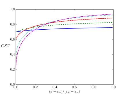
Figure 3: CSC efficiency as function of the difference of Fermi energy with respect to the lower edge $\varepsilon_{-}$ of the spin-helical regime, normalized to the energy interval $\varepsilon_{+}-\varepsilon_{-}$ of the same regime. The $T$-matrix expansion parameter, relevant for the skewness of the potential, is fixed to $(\lambda/\varepsilon)g_{ss}=0.1$. All energies are measured in units of the Rashba SOC $\lambda$. The various curves are for different values of the spin-valley coupling: $\lambda_{sv}=0.1\lambda$ (dot-dashes, magenta), $\lambda_{sv}=0.2\lambda$ (dotted, light blue), $\lambda_{sv}=0.4\lambda$ (long-dashes, red), $\lambda_{sv}=0.6\lambda$ (short-dashes, green), $\lambda_{sv}=0.8\lambda$ (full, blue)

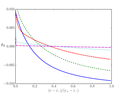
Figure 4: Spin Hall angle as function of the difference of Fermi energy with respect to the lower edge $\varepsilon_{-}$ of the spin-helical regime, normalized to the energy interval $\varepsilon_{+}-\varepsilon_{-}$ of the same regime. All parameters as in fig. 3. The vanishing at $\varepsilon=\lambda$, irrespective of the value of the spin-valley coupling, occurs at different values in terms of normalized variable $(\varepsilon-\varepsilon_{-})/(\varepsilon_{+}-\varepsilon_{-})$ and precisely at 0.473, 0.442, 0.366, 0.269, 0.147 for $\lambda_{sv}=$0.1, 0.2, 0.4, 0.6, 0.8, respectively.

For the SHE, we introduce similarly the spin Hall angle (SHA) $\theta_{H}$

$$\theta_{H}=(e/\hbar)\sigma_{yx}^{z}/\sigma_{xx}.$$ (72)

In the numerical analysis to be presented below, we will express all energies in units of $\lambda$. The disorder enters through the standard combination $\varepsilon\tau/\hbar$ and the coupling constant $g_{ss}$ defined in Eq.(58). For a more extended discussion see Appendix E. The equations (67-69) clearly show the different role played by the effective vertices and transport times in determining the behavior of the physical observables. The effective vertices depend only on the sublattice-spin entangled nature of the eigenstate (6). The analytic expression of the transport times $\tau_{\parallel}$ and $\tau_{\perp}$, which can be obtained by inserting Eqs. (7-9) in Eqs.(63-64), is too cumbersome to be presented here, although their numerical evaluation is straightforward.

The skew-scattering rate $\tau_{a}^{-1}$ shows a characteristic sign change upon increasing the Fermi energy. Such a sign change can be recognized by looking at the analytical expression (64). When the Fermi energy matches exactly the BR energy scale, i.e. $|\varepsilon|=|\lambda|$, the coefficients of the eigenvector (6) acquire a simple expression

$$\alpha=-\frac{\lambda+\lambda_{sv}}{\sqrt{3\lambda^{2}+\lambda_{sv}^{2}}},\beta=\frac{\lambda-\lambda_{sv}}{\sqrt{3\lambda^{2}+\lambda_{sv}^{2}}},\gamma=-1,$$ (73)

which implies the vanishing of the factor $1-\gamma^{2}$, in the formula (64) for the microscopic rate $\tau_{a}^{-1}$. Hence, remarkably, the sign change occurs at a well defined energy when the structure of the eigenvector implies the vanishing of the skew scattering already in lowest order for the effective scattering amplitude in the eigenstates (cf. Eq.(76) and the discussion in Appendix C). In this respect it is illuminating to notice the following equilibrium average

$$\langle\Phi(k_{F},\theta)|\sigma_{0}s_{z}+\sigma_{z}s_{0}|\Phi(k_{F},\theta)\rangle=2(1-\gamma^{2}),$$ (74)

i.e. the factor controlling the sign change, is the equilibrium average of the z-axis component of the total internal angular momentum, which includes both spin and pseudo spin. A change of sign as function of the Fermi energy was also observed for the anomalous Hall effect of Dirac fermions in (Offidani_2018c, ), where it was interpreted in terms of the behavior of the equilibrium spin texture of eigenstates.

Figure 3 shows the Fermi energy dependence of the CSC efficiency. It is apparent that the figure of merit increases monotonically with the carrier density within the spin-helical regime, attaining a maximum at $|\varepsilon|=\varepsilon_{+}$. In regime II, the CSC efficiency decreases monotonically with the Fermi energy $|\varepsilon|$ (Offidani_2017, ) due to the presence of two bands with opposite spin texture. Hence the upper edge $\varepsilon=\pm\varepsilon_{+}$ (for electrons/holes) sets the Fermi energy at which the inverse spin galvanic effect is the most efficient. Upon increasing the spin-valley coupling, there is an interesting effect depending on the charge carrier density. Near the edge of the spin-minority band ($\varepsilon_{+}$), the spin-valley coupling reduces the CSC efficiency, with an opposite effect observed near the lower edge where the “Mexican hat” feature develops (see Fig. 1 (c)). Such a behavior correlates well with the two different-sign regimes for the SHA (see Fig. 4). The latter changes from positive to negative upon increasing the Fermi energy $|\varepsilon|$, which is a consequence of the sign change in the microscopic scattering rate $\tau_{a}^{-1}$ previously discussed and occurs when the Fermi energy matches the Rashba SOC.

In the spin precession measurements reported in Ref. (Benitez_2020, ), the spin galvanic nonlocal resistance ($R_{\textrm{SGE}}$) in a graphene/WS₂ lateral device indeed shows a maximum, in absolute value, as function of the back-gate voltage ($V_{g}$) for both charge carrier polarities. Considering that the charge-neutrality point in the experiment is approximately located at $V_{g}\approx-10$ V and the nonlocal signal maximum (for electrons) at $V_{g}\approx-5$ V, one may estimate a charge carrier density $n\approx 3.5\times 10^{11}\>\mathrm{cm}^{-2}$ at the upper edge of the spin-helical regime (see, for example, Ref. (Ferreira11, )). Using the relation between electronic density and Fermi wavevector for regime I ($n=k_{F}^{2}/2\pi$), we find $\varepsilon_{+}\approx 60$ meV. By reasonably assuming $\lambda_{\textrm{sv}}\ll\lambda$ (in accord with a recent study (Pezo_2020, )), one can further estimate $\lambda\approx 29$ meV. This is a somewhat suprising result, given that functional theory calculations predict a proximity-induced BR SOC on the order of 0.4 meV (Pezo_2020, ; Gmitra_2016, ). In contrast, our estimate compares well with recent quantum Hall effect measurements indicating $\lambda\approx 15$ meV in graphene/WSe₂ (Wang_21, ). Strictly speaking, our estimate should be understood as an upper bound to the true BR SOC energy scale since the gate voltage dependence of $R_{\textrm{SGE}}$ also reflects the spin diffusion within the channel, which tends to shift the nonlocal signal maxima towards higher gate voltages $|V_{g}|$ (see also Ref. (Lin_2020, )). Most importantly, the very evidence of a maximum in $|R_{\textrm{SGE}}|$ as a function of carrier density shows that the spin-helical regime is experimentally accessible. Moreover, the qualitative behavior of the CSC efficiency (unlike the spin Hall angle (Offidani_2018c, )) is little sensitive to microscopic details of the impurity potential (Offidani_2017, ). This provides extra confidence that the behavior of the spin galvanic nonlocal signal in Ref. (Benitez_2020, ) is a fingerprint of emergent spin-helical Dirac fermions at the graphene/TMD interface. On the other hand, a sign change in the SHE signal as the back-gate voltage is swept at fixed carrier polarity as predicted here (see Fig. 4) is not evident in the experimental data (Benitez_2020, ). The significant uncertainty in the nonlocal signal at low temperatures renders a quantitative comparison between theory and experiment more challenging. According to our theory, the sign change occurs when $|\varepsilon|=|\lambda|\approx 29$ meV. Incidentally, the latter roughly coincides with the energy scale of electron-hole puddles in the experiment $\delta E=\hbar v\sqrt{\pi\delta n}$ (with $\delta n\approx 2.5\times 10^{11}\>\textrm{cm}^{-2}$ the residual carrier density), which could smear out the features of the extrinsic SHE predicted here. Therefore, the sign change in the SHA, if observed in cleaner samples, could provide a direct measure of the BR SOC energy scale. Both features, i.e. the maximum in the CSC efficiency and the sign change in SHA, thus provide valuable transport fingerprints of the spin-helical regime realized in graphene with proximity-induced SOC.

We briefly comment on the validity of our microscopic formulation. Close to the charge neutrality point, a full self-consistent evaluation of the self-energy is required to account for the behavior of the longitudinal charge conductivity. Because the weak-disorder condition implies $\epsilon\tau_{\parallel}\gtrsim 10$, which requires not too low carrier density, one needs also a very large SOC to have the regime I spanning a reasonable energy range. Notwithstanding, the predicted sign change in the SHA at $|\varepsilon|\approx|\lambda|$ should be generally valid irrespective of the level at which the self-energy is evaluated and may provide and experimental test of the theory. A detailed self-consistent evaluation to extend our theory closer to the charge neutrality point remains an important development for future work, but is beyond the scope of the present paper.

VII Conclusions

In conclusion, we developed a microscopic theory that captures the key features of coupled spin-charge transport in graphene-based heterostructures, in which Dirac fermions experience proximity-induced spin-valley coupling as well as Bychkov-Rashba effect due to interfacial breaking of inversion symmetry. We have restricted ourselves to the spin-helical regime realized at low electronic densities, characterized by the locking of spin and pseudospin degrees of freedom. Such a simplification has allowed us to derive, within the framework of the Eilenberger equation for the quasiclassical Green’s function, a single transport equation capturing the low-energy behavior of dirty spin-orbit-coupled Dirac fermions. The Eilenberger equation exhibits a scattering kernel, which is derived within a T-matrix expansion by projecting the disorder potential in the energy eigenstate at the Fermi energy. Both symmetric and skew scattering features have been connected to the spin and pseudo spin texture of the eigenstate through explicit analytical expressions. The spin-charge transport response functions are described in terms of longitudinal ($\tau_{\parallel}$) and transverse ($\tau_{\perp}$) transport times. The transverse transport time is different from zero only in the presence of both Bychkov-Rashba interaction and spin-valley coupling, in accord with the exact covariant conservation laws of the Dirac-Rashba model (Milletari_2017, ). Interestingly, the SHE vanishes, then changing sign, when the Fermi energy crosses the Bychkov-Rashba energy scale, irrespective of the value of the spin-valley coupling. This is a consequence of the fact that the equilibrium spin and pseudo spin texture, at this particular value of the Fermi energy, implies a vanishing total spin angular momentum. In the spin-helical energy range, the inverse spin galvanic effect has a maximum at the edge of the spin-minority band. These features then represent the fingerprints of the spin-helical regime and may provide a direct way to estimate the proximity-induced SOC in graphene heterostructures using spin precession measurements in nonlocal geometry that can disentangle SHE and inverse spin galvanic signals (Cavill_2020, ). The comparison with recent experimental results (Benitez_2020, ) provides a reasonable estimate for the Bychkov-Rashba SOC parameter. More importantly, the energy range within which the theory is valid appears to be experimentally accessible, so that the results presented in this paper can be put to a test.

Appendix A Details on gradient expansion

To clarify the procedure, we can consider the simplest possible example: free electrons in a perfect (no disorder) system and in the presence of an electric field described by a scalar potential. We start from the Dyson equation Eq.(12) and move to Wigner coordinates. A convolution product $A(1,2)\otimes B(2,1^{\prime})$ in Wigner space can be written as

$$(A\otimes B)(X,k)=e^{i(\partial_{X}^{A}\partial_{k}^{B}-\partial_{k}^{A}\partial_{X}^{B})}A(X,k)B(X,k)$$

where the coordinates $(X,k)$ define the so-called mixed representation. Here $k=(\mathbf{k,\omega})$. If $A(X,k)$ and $B(X,k)$ are slowly varying functions of $X$, the exponential can be expanded order by order in the small parameter $\partial_{X}\partial_{k}\ll 1$. One can ultimately generates from the Eq.(12) an approximated equation. In the lowest-order approximation of gradient expansion, we have

$$e^{i(\partial_{X}^{A}\partial_{k}^{B}-\partial_{k}^{A}\partial_{X}^{B})/2}\approx 1+\frac{i}{2}(\partial_{X}^{A}\partial_{k}^{B}-i\partial_{k}^{A}\partial_{X}^{B}),$$

so, beyond the standard semiclassical assumption that the potential varies slowly in space and time on the scale set by $1/k_{F},1/\varepsilon$, one has

$$-i\left[\hat{G}_{0}^{-1},^{\otimes}\hat{G}\right]\approx\qquad\qquad\qquad$$

$$\approx\partial_{T}\hat{G}-e\partial_{T}\Phi\partial_{\epsilon}G-\nabla_{\boldsymbol{p}}\hat{G}_{0}^{-1}\cdot\nabla_{\boldsymbol{R}}\hat{G}_{0}^{-1}\cdot\nabla_{\boldsymbol{k}}\hat{G}=$$

$$=\partial_{T}\hat{G}-e\partial_{T}\Phi\partial_{\epsilon}G+\boldsymbol{v}\cdot\nabla_{\boldsymbol{R}}\hat{G}+e\nabla_{\boldsymbol{R}}\Phi(\boldsymbol{R})\cdot\nabla_{\boldsymbol{k}}\hat{G}$$

where $\hat{G}=\hat{G}(X,k)$, $\boldsymbol{v}=\boldsymbol{k}/m$, $\Phi$ is the scalar potential as function of the Wigner variable $\boldsymbol{R}$. From that, after some simple algebra, one can recover the Eq.(15).

Appendix B On the detailed balance

To see better how the detailed balance is obeyed in the picture presented in this work, we have to start from $I_{in}$ and $I_{out}$ terms (the Eq.(24) and the Eq.(20)). They read

$$I_{in}=iu_{0}^{2}\int_{{\bf k^{\prime}}}\Big{(}G_{\mathbf{k}}^{R}\overline{T}^{R}G_{{\bf k^{\prime}}}^{K}\overline{T}^{A}-\overline{T}^{R}G_{{\bf k^{\prime}}}^{K}\overline{T}^{A}G_{\mathbf{k}}^{A}\Big{)}$$

and

$$I_{out}=-iu_{0}^{2}\int_{{\bf k^{\prime}}}\Big{(}G_{{\bf k^{\prime}}}^{R}\overline{T}^{R}G_{\mathbf{k}}^{K}-G_{\mathbf{k}}^{K}G_{{\bf k^{\prime}}}^{A}\overline{T}^{A}\Big{)}.$$

Now, we focus on $I_{out}$ term and project it in the basis in which $G^{R(A)}$ (and then also $\overline{T}^{R(A)}$) is diagonal. So, the $(ij)$-element reads

$$(I_{out})_{ij} = -iu_{0}^{2}\int_{{\bf k^{\prime}}}\Big{(}G_{{\bf k^{\prime}},i}^{R}\overline{T}_{i}^{R}G_{\mathbf{k},(ij)}^{K}-G_{\mathbf{k},(ij)}^{K}G_{{\bf k^{\prime}},j}^{A}\overline{T}_{j}^{A}\Big{)}$$

$$= -iu_{0}^{2}\int_{{\bf k^{\prime}}}G_{\mathbf{k},(ij)}^{K}\Big{(}G_{{\bf k^{\prime}},i}^{R}\overline{T}_{i}^{R}-G_{{\bf k^{\prime}},j}^{A}\overline{T}_{j}^{A}\Big{)}.$$

One can rewrite it as

$$(I_{out})_{ij} = -iu_{0}^{2}G_{\mathbf{k},(ij)}^{K}\Big{(}\frac{G_{{\bf k^{\prime}},i}^{R}}{1-u_{0}G_{{\bf k^{\prime}},i}^{R}}-\frac{G_{{\bf k^{\prime}},j}^{A}}{1-u_{0}G_{{\bf k^{\prime}},j}^{A}}\Big{)}$$

$$= -iu_{0}^{2}G_{\mathbf{k},(ij)}^{K}\Big{(}G_{{\bf k^{\prime}},i}^{R}-G_{{\bf k^{\prime}},j}^{A}\Big{)}\overline{T}_{i}^{R}\overline{T}_{j}^{A}.$$

From this result, we can recover the matrix relation for the $out-$term being careful about the position of each element. In particular one obtains

$$I_{out}=-iu_{0}^{2}\int_{{\bf k^{\prime}}}\Big{(}G_{{\bf k^{\prime}}}^{R}\overline{T}^{R}G_{\mathbf{k}}^{K}\overline{T}^{A}-\overline{T}^{R}G_{\mathbf{k}}^{K}\overline{T}^{A}G_{{\bf k^{\prime}}}^{A}\Big{)}.$$

The latter expression has the same matrix structure of the $in-$relation, as expected.

Appendix C Effective potential in the $C_{6v}$-invariant model

We recall that in this case $\alpha=-\beta=-\varepsilon/\sqrt{\varepsilon(\varepsilon+2\lambda)}$, $\gamma=-1$. Hence the normalization of the eigenvector (6) reads

$$1+\alpha^{2}+\beta^{2}+\gamma^{2}=4\frac{\varepsilon+\lambda}{\varepsilon+2\lambda}.$$ (75)

Although the disorder potential does not have a dependence on the scattering angle, its projection on the energy eigenstates gives rise to such a dependence. To this end we define the scattering amplitude for eigenstates at the Fermi surface with wave vector $\mathbf{k}=k_{F}\mathbf{n}$ and $\mathbf{k^{\prime}}=k_{F}\mathbf{n^{\prime}}$ where $\mathbf{n}=\left(\cos\theta,\sin\theta\right)$ and similarly for $\mathbf{n^{\prime}}$

$$p(\theta,\theta^{\prime}) \equiv \langle\Phi(k_{F},\theta)|\Phi(k_{F},\theta^{\prime})\rangle.$$ (76)

$$= e^{i(\theta-\theta^{\prime})}+\alpha^{2}+\beta^{2}+\gamma^{2}e^{-i(\theta-\theta^{\prime})}$$

$$= \alpha^{2}+\beta^{2}+\mathbf{n}\cdot\mathbf{n^{\prime}}\left(1+\gamma^{2}\right)$$

$$+ i\mathbf{n}\times\mathbf{n^{\prime}}\cdot\mathbf{z}\left(1-\gamma^{2}\right).$$

One sees how the skew scattering in the last term in the right hand side arises from the projection. In the $C_{6v}$-invariant model when $\gamma=-1$ skew scattering is absent in lowest order in the scattering amplitude and cannot appear in any successive order. To evaluate the scattering kernel we then need the trace

$${\rm Tr}\left[P(\theta)P(\theta^{\prime})\right]$$

$$= \frac{p\left(\theta,\theta^{\prime}\right)p\left(\theta^{\prime},\theta\right)}{\left(1+\alpha^{2}+\beta^{2}+\gamma^{2}\right)^{2}}$$

$$= \frac{(\varepsilon+(\varepsilon+2\lambda)\cos(\vartheta))^{2}}{(\varepsilon-\lambda)^{2}},$$

where $\vartheta=\theta-\theta^{\prime}$ as usual and in the last line we used the expressions for $\alpha,\beta,\gamma$ given above. Finally, by recalling that $N_{F}/N_{0}=(\varepsilon+\lambda)/\varepsilon$ and the definition (37) of the scattering kernel, one obtains

$$W(\vartheta)=\frac{1}{\tau}\frac{(\varepsilon+(\varepsilon+2\lambda)\cos(\vartheta))^{2}}{\varepsilon(\varepsilon+\lambda)},$$ (78)

which is the result quoted in the main text.

Appendix D Expression of the effective potential and transport times in the $C_{3v}$-invariant model

We want to find the expressions of the scattering kernel in the general case in terms of the eigenvector coefficients defined in Eq.(6). The Born approximation and skew scattering contributions are defined in Eqs. (44) and (57), respectively. For the scattering kernel in the Born approximation we need, apart from the eigenvector normalization factors,

$${\rm Tr}\left(P(\theta)P(\theta^{\prime})\right) = p(\theta,\theta^{\prime})p(\theta^{\prime},\theta).$$

By defining as usual $\vartheta=\theta-\theta^{\prime}$ and taking the $(1-\cos(\vartheta))$-component as requested by Eq.(61)

$$2\left(-\left(\gamma^{2}+1\right)\left(\alpha^{2}+\beta^{2}\right)+\left(\alpha^{2}+\beta^{2}\right)^{2}+\gamma^{4}+1\right).$$ (79)

In a similar way for the scattering kernel relevant for the skew scattering

$$-i{\rm Tr}\left(\langle P(\theta^{\prime\prime})\rangle\left[P(\theta),P(\theta^{\prime})\right]\right)$$

$$= 2{\rm Im}\int_{0}^{2\pi}\frac{d\theta^{\prime\prime}}{2\pi}p(\theta^{\prime\prime},\theta)p(\theta,\theta^{\prime})p(\theta^{\prime},\theta^{\prime\prime}).$$

After integrating over $\theta^{\prime\prime}$ and setting $\vartheta=\theta-\theta^{\prime}$, we may consider the $\sin(\vartheta)$ component as requested by Eq.(62)

$$2\left(\gamma^{2}-1\right)\left(\alpha^{2}+\beta^{2}\right)\left(\alpha^{2}+\beta^{2}-\gamma^{2}-1\right).$$ (80)

We finally have the transport times expressed in terms of the components of the eigenvector, where we have inserted back the normalization factors,

$$\frac{\tau}{\tau_{s}} = \frac{N_{F}}{N_{0}}\frac{2\left(\gamma^{4}+1+(\alpha^{2}+\beta^{2})(\alpha^{2}+\beta^{2}-\gamma^{2}-1)\right)}{(1+\alpha^{2}+\beta^{2}+\gamma^{2})^{2}},$$

$$\frac{\tau}{\tau_{a}} = g_{ss}\left(\frac{N_{F}}{N_{0}}\right)^{2}\frac{2\left(1-\gamma^{2}\right)\left(\alpha^{2}+\beta^{2}\right)\left(\alpha^{2}+\beta^{2}-\gamma^{2}-1\right)}{(1+\alpha^{2}+\beta^{2}+\gamma^{2})^{3}}.$$

Appendix E Disorder parameters

In numerically evaluating the physical observables we need to fix the strength of the disorder potential, which enters in the expression of the scattering time and of the coupling constant controlling the expansion about the Born approximation. They are, after reinstating $\hbar$,

$$\frac{1}{\tau} = \frac{2\pi}{\hbar}N_{0}n_{imp}u_{0}^{2}=\frac{2\varepsilon}{\hbar}\left(\frac{u_{0}}{v\hbar}\right)^{2}n_{imp},$$ (81)

$$g_{ss} = 2\pi N_{0}u_{0}=2\frac{\varepsilon}{v\hbar}\frac{u_{0}}{v\hbar}.$$ (82)

The theory is valid in the limit $\varepsilon\tau/\hbar\gg 1$ and for $g_{ss}\ll 1$. The quantity $u_{0}/(v\hbar)$ defines a typical length associated with the scattering potential. For typical scattering $u_{0}=1{\rm eV}{\rm nm}^{2}$, one has $u_{0}/(v\hbar)\sim 10^{-9}{\rm cm}$. For energies $\varepsilon\sim 100{\rm meV}$, $\varepsilon/(v\hbar)\sim 10^{6}{\rm cm}^{-1}$ and the weak scattering condition $g_{ss}\ll 1$ is satisfied. With impurity density $n_{imp}=10^{12}{\rm cm}^{-2}$, also the good metal condition is verified. In the numerical plots we use the Rashba SOC $\lambda$ as unit of energy. By indicating with $R=10^{-7}{\rm cm}$ the range of the impurity potential such that $u_{0}=UR^{2}$, we may express the two above disorder parameters as

$$\frac{\hbar}{\lambda\tau} = 2\frac{\varepsilon}{\lambda}\left(\frac{U}{\lambda}\right)^{2}\left(\frac{\lambda R^{2}}{v\hbar}\right)^{2}n_{imp},$$ (83)

$$g_{ss} = 2\frac{\varepsilon}{\lambda}\frac{U}{\lambda}\frac{\lambda}{v\hbar}\frac{\lambda R^{2}}{v\hbar}.$$ (84)

We take $\lambda=10{\rm meV}$ and $v=10^{8}{\rm cm}\>\textrm{s}^{-1}$ so that

$$\frac{\hbar}{\lambda\tau} = 1.8\times 10^{-3}\frac{\varepsilon}{\lambda}$$ (85)

$$g_{ss} = 1.8\times 10^{-2}\frac{\varepsilon}{\lambda}.$$ (86)

The two above relations fix the value of the disorder parameters in terms of the Fermi energy.

References

- (1) A. K. Geim and I. V. Grigorieva, Van der Waals heterostructures, Nature 499, 419 (2013).
- (2) W. Han, R. K. Kawakami, M. Gmitra, J. Fabian, Graphene spintronics, Nat. Nanotech. 9, 794 (2014).
- (3) A. Avsar, H. Ochoa, F. Guinea, B. Özyilmaz, B. J. van Wees, and I. J. Vera-Marun, Colloquium: Spintronics in graphene and other two-dimensional materials. Rev. Mod. Phys. 92, 021003 (2020).
- (4) S. A. Cavill, C. Huang, M. Offidani, Y.-H. Lin, M. A. Cazalilla, and A. Ferreira, Proposal for Unambiguous Electrical Detection of Spin-Charge Conversion in Lateral Spin Valves, Phys. Rev. Lett. 124, 236803 (2020).
- (5) N. Tombros, C. Jozsa, M. Popinciuc, H. T. Jonkman and B. J. van Wees, Electronic spin transport and spin precession in single graphene layers at room temperature, Nature 448, 571 (2007).
- (6) M. H. D. Guimares, A. Veligura, P. J. Zomer, T. Maassen, I. J. Vera-Marun, N. Tombros, and B. J. van Wees. Spin Transport in High-Quality Suspended Graphene Devices, Nano Lett. 12, 3512 (2012).
- (7) M. V. Kamalakar, C. Groenveld, A. Dankert and S. P. Dash, Long distance spin communication in chemical vapour deposited graphene, Nature Comm. 6, 6766 (2015).
- (8) M. Drögeler, C. Franzen, F. Volmer, T. Pohlmann, L. Banszerus, M.Wolter, K. Watanabe, T. Taniguchi, C. Stampfer, and B. Beschoten, Spin lifetimes exceeding 12 nanoseconds in graphene non-local spin valve devices, Nano Lett. 16, 3533 (2016)
- (9) Z. M. Gebeyehu, S. Parui, J. F. Sierra, M. Timmermans, M. J. Esplandiu, S. Brems, C. Huyghebaert, K. Garello, M. V. Costache and S. O. Valenzuela. Spin communication over 30 µm long channels of chemical vapor deposited graphene on SiO2, 2D Mater. 6, 034003 (2019).
- (10) A. Ferreira, T. G. Rappoport, M. A. Cazalilla, and A. H. Castro Neto, Extrinsic Spin Hall Effect Induced by Resonant Skew Scattering in Graphene, Phys. Rev. Lett. 112, 066601 (2014).
- (11) J. Balakrishnan, G. K. W. Koon, A. Avsar, Y. Ho, J. H. Lee, M. Jaiswal, S.-J. Baeck, J.-H. Ahn, A. Ferreira, M. A. Cazalilla, A. H. Castro Neto and B. Özyilmaz, Giant spin Hall effect in graphene grown by chemical vapour deposition, Nature Comm. 5, 4748 (2014).
- (12) D. V. Tuan, J. M. M.-Tejada, X. Waintal, B. K. Nikolić, S. O. Valenzuela, and S. Roche, Spin Hall Effect and Origins of Nonlocal Resistance in Adatom-Decorated Graphene, Phys. Rev. Lett. 117, 176602 (2016).
- (13) A. Pachoud, A. Ferreira, B. Özyilmaz, and A. H. Castro Neto, Scattering theory of spin-orbit active adatoms on graphene, Phys. Rev. B 90, 035444 (2014).
- (14) C. Huang, Y. D. Chong, and M. A. Cazalilla, Direct coupling between charge current and spin polarization by extrinsic mechanisms in graphene, Phys. Rev. B 94, 085414 (2016).
- (15) A. Avsar, J. Y. Tan, T. Taychatanapat, J. Balakrishnan, G.K.W. Koon, Y. Yeo, J. Lahiri, A. Carvalho, A. S. Rodin, E. C. T. O Farrell, G. Eda, A. H. Castro Neto, B. Ozyilmaz, Spin–orbit proximity effect in graphene, Nat. Commun. 5, 4875 (2014).
- (16) Z. Wang, D.-K. Ki, H. Chen, H. Berger, A. H. MacDonald, and A. F. Morpurgo, Strong interface-induced spin–orbit interaction in graphene on WS2, Nat. Commun. 6, 8339 (2015).
- (17) M. Gmitra and J. Fabian, Graphene on transition-metal dichalcogenides: A platform for proximity spin-orbit physics and optospintronics, Phys. Rev. B 92, 155403 (2015).
- (18) M. Offidani, M. Milletarì, R. Raimondi, and A. Ferreira, Optimal Charge-to-Spin Conversion in Graphene on Transition-Metal Dichalcogenides, Phys. Rev. Lett. 119, 196801 (2017).
- (19) J. O. Island, X. Cui, C. Lewandowski, J. Y. Khoo, E. M. Spanton, H. Zhou, D. Rhodes, J. C. Hone, T. Taniguchi, K. Watanabe, L. S. Levitov, M. P. Zaletel, and A. F. Young, Spin-orbit-driven band inversion in bilayer graphene by the van der Waals proximity effect, Nature 571, 85 (2019).
- (20) D. Wang, S. Che, G. Cao, R. Lyu, K. Watanabe, T. Taniguchi, C. N. Lau, and M. Bockrath, Quantum Hall Effect Measurement of Spin–Orbit Coupling Strengths in Ultraclean Bilayer Graphene/WSe2 Heterostructures, Nano Lett. 19, 7028 (2019).
- (21) J.-X. Lin, Y.-H. Zhang, E. Morissette, Z. Wang, S. Liu, D. Rhodes, K. Watanabe, T. Taniguchi, J. Hone, J.I.A. Li, Proximity-induced spin-orbit coupling and ferromagnetism in magic-angle twisted bilayer graphene, arXiv:2102.06566 (2021).
- (22) Y. A. Bychkov and E. I. Rashba, Properties of a 2D electron gas with lifted spectral degeneracy, JETP Lett. 39, 78 (1984).
- (23) E. I. Rashba, Graphene with structure-induced spin-orbit coupling: Spin-polarized states, spin zero modes, and quantum Hall effect, Phys. Rev. B 79, 161409(R) (2009).
- (24) D. Marchenko, A. Varykhalov, M. R. Scholz, G. Bihlmayer, E. I. Rashba, A. Rybkin, A. M. Shikin, O. Rader, Giant Rashba splitting in graphene due to hybridization with gold, Nat. Commun. 3, 1232 (2012).
- (25) M. Offidani and A. Ferreira, Anomalous Hall Effect in 2D Dirac Materials, Phys. Rev. Lett. 121, 126802 (2018).
- (26) D. Huertas-Hernando, F. Guinea, A. Brataas, Spin-Orbit-Mediated Spin Relaxation in Graphene, Phys. Rev. Lett. 103, 146801 (2009).
- (27) M. Gmitra, D. Kochan, P. Hogl and J. Fabian, Trivial and inverted Dirac bands and the emergence of quantum spin Hall states in graphene on transition-metal dichalcogenides, Phys. Rev. B 93, 155104 (2016).
- (28) F. J. dos Santos, D. A. Bahamon, R. B. Muniz, K. McKenna, E. V. Castro, J. Lischner, and A. Ferreira, Impact of complex adatom-induced interactions on quantum spin Hall phases, Phys. Rev. B 98, 081407(R) (2018).
- (29) T. P. Cysne, A. Ferreira and T. Rappoport, Crystal-field effects in graphene with interface-induced spin-orbit coupling, Phys. Rev. B 98, 045407 (2018).
- (30) J. Xu, T. Zhu, Y. K. Luo, Y.-M. Lu, and R. K. Kawakami, Strong and Tunable Spin-Lifetime Anisotropy in Dual-Gated Bilayer Graphene, Phys. Rev. Lett. 121, 127703 (2018).
- (31) J. C. Leutenantsmeyer, J. Ingla-Aynés, J. Fabian, and B. J. van Wees, Observation of Spin-Valley-Coupling-Induced Large Spin-Lifetime Anisotropy in Bilayer Graphene, Phys. Rev. Lett. 121, 127702 (2018).
- (32) Z. Wang, D.-K. Ki, J. Y. Khoo, D. Mauro, H. Berger, L. S. Levitov, and A. F. Morpurgo, Origin and Magnitude of ‘Designer’ Spin-Orbit Interaction in Graphene on Semiconducting Transition Metal Dichalcogenides, Phys. Rev. X 6, 041020 (2016).
- (33) B. Yang, M. Lohmann, D. Barroso, I. Liao, Z. Lin, Y. Liu, L. Bartels, K. Watanabe, T. Taniguchi, J. Shi, Strong electron-hole symmetric Rashba spin-orbit coupling in graphene/monolayer transition metal dichalcogenide heterostructures, Phys. Rev. B 96, 041409 (2017).
- (34) T. Völkl, T. Rockinger, M. Drienovsky, K. Watanabe, T. Taniguchi, D. Weiss, and J. Eroms, Magnetotransport in heterostructures of transition metal dichalcogenides and graphene, Phys. Rev. B 96, 125405 (2017).
- (35) S. Zihlmann, A. W. Cummings, J. H. Garcia, M. Kedves, K. Watanabe, T. Taniguchi, C. Schönenberger, and P. Makk, Phys. Rev. B 97, 075434 (2018).
- (36) T. Wakamura, F. Reale, P. Palczynski, S. Guron, C. Mattevi, and H. Bouchiat, Strong Anisotropic Spin-Orbit Interaction Induced in Graphene by Monolayer WS2, Phys. Rev. Lett. 120, 106802 (2018).
- (37) J. Sichau, M. Prada, T. Anlauf, T. J. Lyon, B. Bosnjak, L. Tiemann, and R. H. Blick, Resonance Microwave Measurements of an Intrinsic Spin-Orbit Coupling Gap in Graphene: A Possible Indication of a Topological State, Phys. Rev. Lett. 122, 046403 (2019).
- (38) L. A. Benitez, J. F. Sierra, W. Savero Torres, A. Arrighi, F. Bonell, M. V. Costache, and S. O. Valenzuela, Strongly anisotropic spin relaxation in graphene–transition metal dichalcogenide heterostructures at room temperature, Nat. Phys. 14, 303 (2017).
- (39) T. S. Ghiasi, J. Ingla-Aynes, A. A. Kaverzin, and B. J. Van Wees, Large Proximity-Induced Spin Lifetime Anisotropy in Transition-Metal Dichalcogenide/Graphene Heterostructures, Nano Lett. 17, 7528 (2017).
- (40) S. Zihlmann, A. W. Cummings, J. H. Garcia, M. Kedves, K. Watanabe, T. Taniguchi, C. Schonenberger, and P. Makk, Large spin relaxation anisotropy and valley-Zeeman spin-orbit coupling in WSe2/graphene/h-BN heterostructures, Phys. Rev. B 97, 075434 (2018).
- (41) A. W. Cummings, J. H. Garcia, J. Fabian, and S. Roche, Giant Spin Lifetime Anisotropy in Graphene Induced by Proximity Effects, Phys. Rev. Lett. 119, 206601 (2017).
- (42) M. Offidani and A. Ferreira, Microscopic theory of spin relaxation anisotropy in graphene with proximity-induced spin-orbit coupling, Phys. Rev. B 98, 245408 (2018).
- (43) C. K. Safeer, J. Ingla-Aynes, F. Herling, J. H. Garcia, M. Vila, N. Ontoso, M. R. Calvo, S. Roche, L. E. Hueso, and F. Casanova, Room-Temperature Spin Hall Effect in Graphene/MoS2 van der Waals Heterostructures, Nano Lett. 19, 1074 (2019).
- (44) T. S. Ghiasi, A. A. Kaverzin, P. J. Blah and B. J. van Wees, Charge-to-Spin Conversion by the Rashba–Edelstein Effect in Two-Dimensional van der Waals Heterostructures up to Room Temperature, Nano Lett. 19, 5959 (2019).
- (45) L. A. Benitez, W. Savero Torres, J. F. Sierra, M. Tim- mermans, J. H. Garcia, S. Roche, M. V. Costache, and S. O. Valenzuela, Tunable room-temperature spin galvanic and spin Hall effects in van der Waals heterostructures, Nat. Materials 19, 170 (2020).
- (46) D. Khokhriakov, A. Md. Hoque, B. Karpiak, S. P. Dash, Gate-tunable spin-galvanic effect in graphene-topological insulator van der Waals heterostructures at room temperature, Nature Comm. 11, 3657 (2020).
- (47) L. Lin, J. Zhang, G. Myeong, W. Shin, H. Lim, B. Kim, S. Kim, T. Jin, S. Cavill, B. S. Kim, C. Kim, J. Lischner, A. Ferreira, and S. Cho, Gate-Tunable Reversible Rashba–Edelstein Effect in a Few-Layer Graphene/2H-TaS2 Heterostructure at Room Temperature, ACS Nano 14, 5251 (2020).
- (48) M. Milletarí and A. Ferreira, Quantum diagrammatic theory of the extrinsic spin Hall effect in graphene, Phys. Rev. B 94, 134202 (2016)
- (49) M. Milletarí and A. Ferreira, Crossover to the anomalous quantum regime in the extrinsic spin Hall effect of graphene, Phys. Rev. B 94, 201402(R) (2016).
- (50) M. Milletarì, M. Offidani, A. Ferreira, and R. Raimondi, Covariant Conservation Laws and the Spin Hall Effect in Dirac-Rashba Systems, Phys. Rev. Lett. 119, 246801 (2017).
- (51) M. Offidani, R. Raimondi, and A. Ferreira, Microscopic Linear Response Theory of Spin Relaxation and Relativistic Transport Phenomena in Graphene, Condens. Matter 3, 18 (2018).
- (52) J.-i. Inoue, G. E. W. Bauer, and L. W. Molenkamp, Suppression of the persistent spin Hall current by defect scattering, Phys. Rev. B 70, 041303(R) (2004).
- (53) E. G. Mishchenko, A. V. Shytov, and B. I. Halperin, Spin Current and Polarization in Impure Two-Dimensional Electron Systems with Spin-Orbit Coupling, Phys. Rev. Lett. 93, 226602 (2004).
- (54) O. V. Dimitrova, Spin-Hall conductivity in a two-dimensional Rashba electron gas, Phys. Rev. B 71, 245327 (2005).
- (55) R. Raimondi, C. Gorini, P. Schwab, and M. Dzierzawa, Quasiclassical approach to the spin Hall effect in the two-dimensional electron gas, Phys. Rev. B 74, 035340 (2006).
- (56) C. Gorini, P. Schwab, R. Raimondi, and A. L. Shelankov, Non-Abelian gauge fields in the gradient expansion: Generalized Boltzmann and Eilenberger equations, Phys. Rev. B 82, 195316 (2010).
- (57) R. Raimondi, P. Schwab, C. Gorini, and G. Vignale, Spin-orbit interaction in a two-dimensional electron gas: A SU(2) formulation, Ann. Phys. (Berlin, Ger.) 524, 153 (2012).
- (58) G. Eilenberger, Transformation of Gorkov’s equation for type II superconductors into transport-like equations, Z. Phys. 214, 195 (1968).
- (59) J. Rammer and H. Smith, uantum field-theoretical methods in transport theory of metals, Rev. Mod. Phys. 58, 323 (1986).
- (60) P. Schwab, R. Raimondi, and C. Gorini, Spin-charge locking and tunneling into a helical metal, Europhys. Lett. 93, 67004 (2011).
- (61) D. Kochan, S. Irmer, and J. Fabian, Model spin-orbit coupling Hamiltonians for graphene systems, Phys. Rev. B 95, 165415 (2017).
- (62) D. V. Tuan, F. Ortmann, D. Soriano, Se. O. Valenzuela and S. Roche, Pseudospin-driven spin relaxation mechanism in graphene, Nat. Physics 10, 857 (2014).
- (63) F. Sousa, G. Tatara, and A. Ferreira, Skew-scattering-induced giant antidamping spin-orbit torques: Collinear and out-of-plane Edelstein effects at two-dimensional material/ferromagnet interfaces, Phys. Rev. Research 2, 043401 (2020).
- (64) C. L. Kane and E. J. Mele, Z2 Topological Order and the Quantum Spin Hall Effect, Phys. Rev. Lett. 95, 146802 (2005).
- (65) C. L. Kane and E. J. Mele, Quantum Spin Hall Effect in Graphene, Phys. Rev. Lett. 95, 226801 (2005).
- (66) A. Srivastava, M. Sidler, A. V. Allain, D. S. Lembke, A. Kis and A. Imamoğlu, Valley Zeeman effect in elementary optical excitations of monolayer WSe2, Nature Physics 11, 141 (2015).
- (67) Pezo, Z. Zanolli, N. Wittemeier, A. Fazzio, S. Roche, and J. H. Garcia, A Twist for Tuning the Spin-orbit Coupling in Graphene/Transition Metal Dichalcogenide Heterobilayer, arXiv:2011.06714 (2020).
- (68) J. Schwinger, Brownian Motion of a Quantum Oscillator, J. Math. Phys. 2, 407 (1961).
- (69) L. V. Keldysh, Diagram Technique for Nonequilibrium Processes, JETP 20, 1018 (1965).
- (70) J. Rammer, Quantum Field Theory of Non-equilibrium States, Cambridge University Press (2007).
- (71) P. Schwab and R. Raimondi, Quasiclassical theory of charge transport in disordered interacting electron systems, Ann. Phys., 12, 471 (2003).
- (72) A. Kamenev and A. Levchenko, Keldysh technique and non-linear sigma-model: basic principles and applications, Advances in Physics 58, 197 (2009).
- (73) R. Raimondi, C. Gorini, S. Tölle, in V. Dugaev, I. Tralle, A. Wal, J. Barnas, eds., Spin Orbitronics and Topological Transport Properties, chap. 5, 80, World Scientific, Singapore (2018).
- (74) L. P. Kadanoff and G. Baym, edited by D. Pines (Westview Press, 1962) p. 224.
- (75) Joel L. Lebowitz, 25 Years of Non-Equilibrium Statistical Mechanics, Springer (1995).
- (76) V.M. Edelstein, Spin polarization of conduction electrons induced by electric current in two-dimensional asymmetric electron systems, Solid State Commun. 73, 233 (1990).
- (77) François Konschelle, Transport equations for superconductors in the presence of spin interaction, Eur. Phys. J. B 87, 119 (2014).
- (78) J. Garcia, A. W. Cummings, and S. Roche, Spin Hall Effect and Weak Antilocalization in Graphene/Transition Metal Dichalcogenide Heterostructures, Nano Lett. 17, 5078 (2017).
- (79) A. Ferreira, J. V.-Gomes, J. Nilsson, E. R. Mucciolo, N. M. R. Peres, and A. H. Castro Neto, Unified description of the dc conductivity of monolayer and bilayer graphene at finite densities based on resonant scatterers, Phys. Rev. B 83, 165402 (2011).