A $(2+\varepsilon)$-Approximation Algorithm for Maximum Independent Set of Rectangles

Abstract

We study the Maximum Independent Set of Rectangles (MISR) problem, where we are given a set of axis-parallel rectangles in the plane and the goal is to select a subset of non-overlapping rectangles of maximum cardinality. In a recent breakthrough, Mitchell [45] obtained the first constant-factor approximation algorithm for MISR. His algorithm achieves an approximation ratio of 10 and it is based on a dynamic program that intuitively recursively partitions the input plane into special polygons called corner-clipped rectangles (CCRs), without intersecting certain special horizontal line segments called fences.

In this paper, we present a $(2+\varepsilon)$-approximation algorithm for MISR which is also based on a recursive partitioning scheme. First, we use a partition into a class of axis-parallel polygons with constant complexity each that are more general than CCRs. This allows us to provide an arguably simpler analysis and at the same time already improves the approximation ratio to 6. Then, using a more elaborate charging scheme and a recursive partitioning into general axis-parallel polygons with constant complexity, we improve our approximation ratio to $2+\varepsilon$. In particular, we construct a recursive partitioning based on more general fences which can be sequences of up to $O(1/\varepsilon)$ line segments each. This partitioning routine and our other new ideas may be useful for future work towards a PTAS for MISR.

1 Introduction

Maximum Independent Set of Rectangles (MISR) is a fundamental and well-studied problem in computational geometry, combinatorial optimization and approximation algorithms. In MISR, we are given a set $\mathcal{R}$ of $n$ possibly overlapping axis-parallel rectangles in the plane. We are looking for a subset $\mathcal{R}^{*}\subseteq\mathcal{R}$ of maximum cardinality such that the rectangles in $\mathcal{R}^{*}$ are pairwise disjoint. MISR finds numerous applications in practice, e.g., in map labeling [36, 25], data mining [28] and resource allocation [43].

The problem is an important special case of the Maximum Independent Set problem in graphs, which in general is NP-hard to approximate within a factor of $n^{1-\varepsilon}$ for any constant $\varepsilon>0$ [35]. However, for MISR much better approximation ratios are possible, e.g., there are multiple $O(\log n)$-approximation algorithms [15, 50, 42]. It had been a long-standing open problem to find an $O(1)$-approximation algorithm for MISR. One possible approach for this is to compute an optimal solution to the canonical LP-relaxation of MISR and round it. This approach was used by Chalermsook and Chuzhoy in order to obtain an $O(\log\log n)$-approximation [16]. The LP is conjectured to have an integrality gap of $O(1)$ which is a long-standing open problem by itself, with interesting connections to graph theory [14, 16]. On the other hand, it seems likely that MISR admits even a PTAS, given that it admits a QPTAS due to Adamaszek and Wiese [3], and in particular one with a running time of only  $n^{O((\log\log n/\varepsilon)^{{4}})}$ due to Chuzhoy and Ene [23].

Recently, in a breakthrough result, Mitchell presented a polynomial time 10-approximation algorithm [45] and consequently solved the aforementioned long-standing open problem. Instead of rounding the LP, he employs a recursive partitioning of the plane into a special type of rectilinear polygons called corner-clipped rectangles (CCRs). Given a CCR, he recursively subdivides it into at most five smaller CCRs until he obtains CCRs which essentially contain at most one rectangle from the optimal solution $\mathrm{OPT}$ each. At the end, he outputs the rectangles contained in these final CCRs plus some carefully chosen rectangles from $\mathrm{OPT}$ that are intersected by these recursive cuts. With a dynamic program, he computes the recursive partition that yields the largest number of output rectangles, which in particular “remembers” in each step $O(1)$ rectangles that were intersected by some previous cuts. In a structural theorem he shows that there exists a set of at least $|\mathrm{OPT}|/10$ rectangles which can be output by such a recursive partitioning, leading to the approximation ratio of 10. The structural theorem is proved using an exhaustive case analysis for defining the subdivision of a given CCR, with sixty cases in total.

Mitchell’s result yields several interesting open questions, most notably whether one can improve the approximation ratio and whether one can give a simpler analysis which does not rely on a large case distinction. In this paper, we answer both questions in the affirmative.

1.1 Our Contribution

In this paper, we present a polynomial time $(2+\varepsilon)$-approximation algorithm for MISR. In a first step, we construct a 6-approximation algorithm which hence already improves the approximation ratio. It uses an arguably simpler analysis, and also a less complicated dynamic program. Similar to the result by Mitchell [45], we use a recursive decomposition of the plane into a constant number of (simple) axis-parallel polygons with constant complexity each. However, instead of requiring the arising polygons to be CCRs, all our polygons are horizontally (or vertically) convex (see Figure 1), i.e., if two points in the polygon lie on the same horizontal (vertical) line, then any point between them is also contained in the polygon, and we require the polygons to have a bounded number of edges. Hence, this class of polygons is larger than CCRs. We prove that we can recursively partition the input plane into polygons of this class, such that at the end we extract at least $|\mathrm{OPT}|/6$ rectangles from $\mathrm{OPT}$. In fact, we can compute such a partition with a simpler dynamic program that does not need to remember any rectangle intersected by previous cuts, but which instead just partitions the plane recursively.

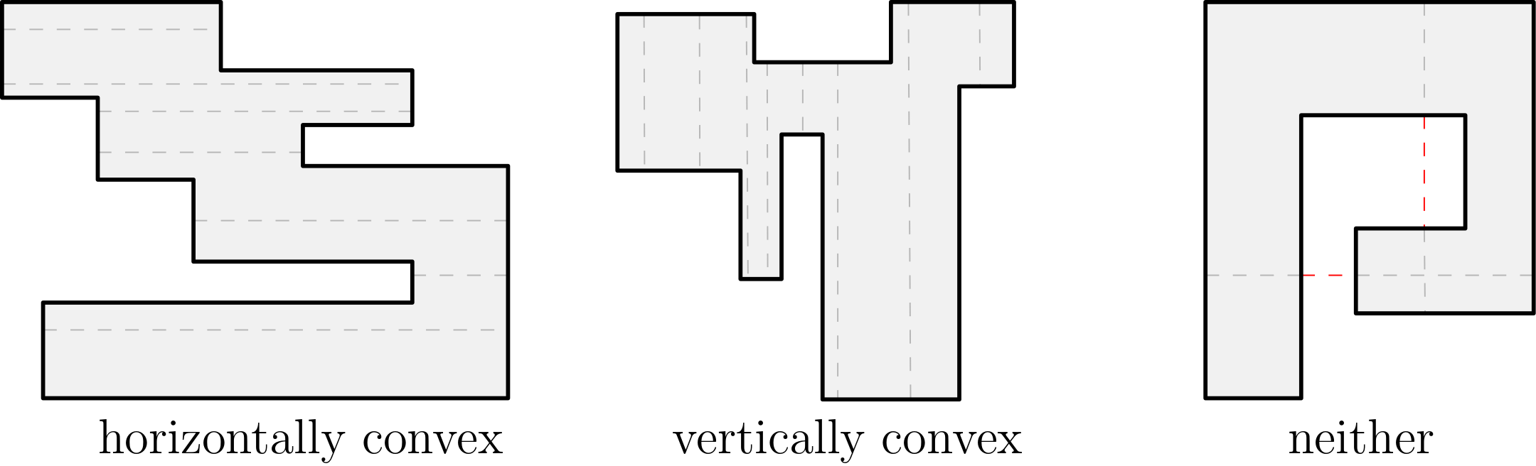
Figure 1: On the left a horizontally convex polygon. On the middle, a vertically convex polygon. On the right, an axis-parallel polygon that is neither horizontally nor vertically convex.

Given a horizontally (or vertically) convex polygon, we show that we can cut it into at most three smaller polygons (with a bounded number of edges), such that the cut uses only one single line segment $\ell$ that potentially intersects rectangles from $\mathrm{OPT}$ (and which are hence lost). In contrast, in [45] there can be two line segments of this type which yields a higher approximation ratio. Note that with this strategy it is unavoidable to intersect some rectangles from $\mathrm{OPT}$ (unless the instance is very easy). However, we ensure that for each rectangle $R\in\mathrm{OPT}$ intersected by $\ell$, we can find two other rectangles from $\mathrm{OPT}$ that we can charge $R$ to, while in [45] there was only one rectangle to charge to. Also, when we define our cut, there are only two different cases that we need to consider, which leads to an arguably simpler analysis. Based on this, we construct a fractional charging scheme which yields an approximation ratio of 6.

We extend this approach to improve the approximation ratio even further. In [45] and in our algorithm above, fences are defined which are horizontal line segments, emerging from boundary edges of the polygon. We are not allowed to cut through them in our recursive partition, and this intuitively protect some rectangles in $\mathrm{OPT}$ from being intersected (in particular the rectangles that we charged other rectangles to). We extend this approach to more general fences, each of them being a sequence of $7$ axis-parallel line segments, rather than single horizontal line segments. Like the fences above, they protect some of the rectangles in $\mathrm{OPT}$ from being deleted, since we do not allow ourselves to cut through them. However, due to their more elaborate shape, they protect more rectangles in $\mathrm{OPT}$ and they protect them better. For example, we use them to ensure that each rectangle receives charge either only from rectangles on its left, or only from rectangles on its right.

We show that in this way we obtain an approximation ratio of 3. Note that in [45] and in our algorithm above the rectangles in $\mathrm{OPT}$ are subdivided into three groups that are denoted as horizontally nested rectangles, vertically nested rectangles, and rectangles that are neither horizontally nor vertically nested. W.l.o.g. we can assume that there are at most $|\mathrm{OPT}|/2$ horizontally nested rectangles, which loses a factor of 2 (in [45] and in our argumentation). However, it turns out that our solution still sometimes contains some horizontally nested rectangles. In this case, we lose less than a factor of 2 in the previous step. Also, in some settings we identify more rectangles to charge to than in the previous argumentation. With these two ingredients we construct a more involved fractional charging argument which improves the approximation ratio to 3. In particular, this charging scheme crucially needs our more general fences in order to distribute the charges appropriately to rectangles that are included in the computed solution.

We need that our recursive partitioning sequence does not intersect any of our more general fences. To this end, we design a new recursive partitioning scheme based on axis-parallel polygons of constant complexity, without imposing additional conditions on the polygons like, e.g., being horizontally convex or a CCR. For our 3-approximation it would be sufficient to have such a scheme for fences with up to 7 line segments each. However, we obtain such a partition even for any set of $x$-monotone fences with an arbitrarily large constant number $\tau\in\mathbb{N}$ of line segments each. This can be used directly as a black-box in future work. For example, it might be that one can design a PTAS for MISR via fences with $\tau=1/\varepsilon^{O(1)}$ many line segments each.

Finally, we show that by using fences with $\tau=O(1/\varepsilon)$ line segments, we improve our approximation ratio to $2+\varepsilon$. To this end, we replace the definition of horizontally and vertically nested rectangles by a related but different definition of horizontally and vertically nice rectangles. This simplifies the analysis since now there are only two groups of rectangles, horizontally nice and vertically nice rectangles. Similar as above, by losing a factor of 2 we assume that at least $|\mathrm{OPT}|/2$ rectangles are horizontally nice. We construct a fractional charging argumentation in which each intersected horizontally nice rectangle is charged either to one vertically nice rectangle in our solution (i.e., that we assumed to be already lost when we focused on the horizontally nice rectangles) or to $1/\varepsilon$ horizontally nice rectangles in our solution. This yields an approximation ratio of $2+\varepsilon$.

We hope that our other new ideas will lead to further progress towards a PTAS for MISR.

Theorem 1.

For any $\varepsilon>0$ there is a polynomial-time $(2+\varepsilon)$-approximation algorithm for the Maximum Independent Set of Rectangles problem.

We remark that in order to obtain a better approximation ratio than 2, substantially new ideas seem to be needed. In the approach by Mitchell [45] as well as in our argumentations, the analysis loses a factor of 2 by focusing on the rectangles that are not horizontally nested or that are horizontally nice, respectively. This loses a factor of 2 in the approximation ratio. It seems unclear how to avoid this.

In parallel and independently from our work, Mitchell recently improved his 10-approximation algorithm to a $10/3$-approximation, and he claims that this algorithm can be improved further to a $(3+\varepsilon)$-approximation whose running time depends on $\varepsilon$ [46].

1.2 Other related work

For simple geometric objects such as disks, squares and fat objects, polynomial-time approximation schemes (PTAS) are known for the corresponding setting of Independent Set [26, 19]. In the weighted case of MISR, each rectangle has an associated weight and the goal is to select a maximum weight independent set. Recently, Chalermsook and Walczak obtained an $O(\log\log n)$-approximation [16], improving the previous $O(\log n/\log\log n)$-approximation by Chan and Har-Peled [19]. Furthermore, Marx [44] showed that MISR is W[1]-hard, ruling out an EPTAS for the problem. Grandoni et al. [32] presented a parameterized approximation scheme for the problem. Fox and Pach [27] have given an $n^{\varepsilon}$-approximation for maximum independent set of line segments. In fact, their result extends to the independent set of intersection graphs of $k$-intersecting curves (where each pair of curves has at most $k$ points in common).

MISR also has interesting connections with end-to-end cuts (called guillotine cuts [51], also known as binary space partitions [24]). Due to its practical relevance in cutting industry, guillotine cuts are well-studied for packing problems, e.g., [9, 40]. It has been conjectured that, given a set of $n$ axis-parallel rectangles, $\Omega(n)$ rectangles can be separated using a sequence of guillotine cuts [1]. If true, this will imply an $O(n^{5})$-time simple $O(1)$-approximation algorithm for MISR [1, 41].

There are many other related important geometric optimization problems, such as Geometric Set Cover [18, 17, 48], Geometric Hitting Set [21, 4, 49], 2-D Bin Packing [6, 37, 8], Strip Packing [34, 38, 29], 2-D Knapsack [39, 30, 31], Unsplittable Flow on a Path [13, 7, 12, 5, 33], Storage Allocation problem [10, 11, 47], etc. We refer the readers to [22] for a literature survey.

2 Dynamic program

We assume that we are given the set $\mathcal{R}$ with $n$ axis-parallel rectangles in the plane such that each rectangle $R\in\mathcal{R}$ is specified by its two opposite corners $(x_{l},y_{b})\in\mathbb{N}^{2}$ and $(x_{r},y_{t})\in\mathbb{N}^{2}$, with $x_{l}<x_{r}$ and $y_{b}<y_{t}$, so that $R:=\{(x,y)\in\mathbb{R}^{2}\mid x_{l}<x<x_{r}\wedge y_{b}<y<y_{t}\}$ (i.e., the rectangles are open sets). By a standard preprocessing [2], we can assume that, for each rectangle $R\in\mathcal{R}$, we have that $x_{l},x_{r},y_{b},y_{t}\in\{0,1,\dots,2n-1\}$. In particular, all input rectangles are contained in the square $S:=[0,2n-1]\times[0,2n-1]$.

Our algorithm is a geometric dynamic program (similar as in [2, 23, 45]) which, intuitively, recursively subdivides $S$ into smaller polygons until each polygon contains only one rectangle from the optimal solution $\mathrm{OPT}$. For each of the latter polygons, it selects one input rectangle that is contained in the polygon, and finally outputs the set of all rectangles that are selected in this way. During the recursion, we ensure that each arising polygon has only $O(1)$ edges that are all axis-parallel with integral coordinates. This ensures that there are only $n^{O(1)}$ possible polygons of this type, which allows us to define a dynamic program that computes the best recursive partition of $S$ in time $n^{O(1)}$. Note that the line segments defining the recursive subdivision of $S$ might intersect rectangles from $\mathrm{OPT}$ and those will not be included in our solution.

Our dynamic program has a parameter $k\in\mathbb{N}$. It has a dynamic programming table with one cell for each simple polygon $P\subseteq S$ with at most $k$ axis-parallel edges, such that the endpoints of each edge have integral coordinates.

Denote by $\mathcal{P}(k):=\mathcal{P}$ the set of polygons corresponding to the DP-cells. For each $P\in\mathcal{P}$, the dynamic program computes a solution $\mathrm{DP}(P)\subseteq\mathcal{R}$ consisting of rectangles from $\mathcal{R}$ contained in $P$. For computing these solutions, we order the polygons in $\mathcal{P}$ according to any partial order $\prec$ in which, for each $P,P^{\prime}\in\mathcal{P}$ with $P\subsetneq P^{\prime}$, it holds that $P\prec P^{\prime}$. We consider the polygons in $\mathcal{P}$ in this order so as to compute their respective solutions $\mathrm{DP}(P)$. Consider a polygon $P\in\mathcal{P}$. If $P$ does not contain any rectangle from $\mathcal{R}$ then we define $\mathrm{DP}(P):=\emptyset$ and stop. Similarly, if $P$ contains only one rectangle $R\in\mathcal{R}$ then we define $\mathrm{DP}(P):=\{R\}$ and stop. Otherwise, the DP tries all subdivisions of $P$ into at most three polygons $P_{1},P_{2},P_{3}\in\mathcal{P}$ with at most $k$ axis-parallel edges each, looks up their corresponding (already computed) solutions and defines their union $\mathrm{DP}(P_{1})\cup\mathrm{DP}(P_{2})\cup\mathrm{DP}(P_{3})$ as a candidate solution for $P$. Finally, we define $\mathrm{DP}(P)$ to be the candidate solution with largest cardinality. At the very end, we output $\mathrm{DP}(S)$.

Lemma 2.

Parameterized by $k\in\mathbb{N}$, the running time of the dynamic program is $O(n^{5k/2})$.

In order to analyze the DP, we introduce the concept of $k$-recursive partitions. Intuitively, the solution computed by the DP corresponds to a recursive partition of $S$ into polygons in $\mathcal{P}$, in which each arising polygon $P$ is further subdivided into at most three polygons $P_{1},P_{2}$ and $P_{3}$, or instead we select at most one rectangle $R\subseteq P$ and do not partition $P$ further. This can be modeled as a tree as given in the following definition.

Definition 3.

A $k$-recursive partition for a set $\mathcal{R}^{\prime}\subseteq\mathcal{R}$ consists of a rooted tree with vertices $V$ such that

• for each node $v\in V$ there is a corresponding polygon $P_{v}\in\mathcal{P}(k)$,

• for the root node $r\in V$ it holds that $P_{r}=S$,

• each internal node $v$ has at most three children $C_{v}\subseteq V$ such that $P_{v}=\dot{\cup}_{v^{\prime}\in C_{v}}P_{v^{\prime}}$,

• for each leaf $v\in V$, $P_{v}$ contains at most one rectangle in $\mathcal{R}^{\prime}$.

• for each rectangle $R^{\prime}\in\mathcal{R}^{\prime}$, there exists a leaf $v\in V$ such that $R^{\prime}\subseteq P_{v}$ and $R^{\prime}\cap P_{v^{\prime}}=\emptyset$ for each leaf $v^{\prime}$ with $v^{\prime}\neq v$.

Note that the rectangles in $\mathcal{R}^{\prime}$ are pairwise disjoint due to the last property. Also, for each internal node $v$, the polygons of its children are disjoint.

Lemma 4.

Given an input set of rectangles $\mathcal{R}$, if there exists a $k$-recursive partition for a set $\mathcal{R}^{\prime}\subseteq\mathcal{R}$, then on input $\mathcal{R}$ our dynamic program computes a solution $\tilde{\mathcal{R}}\subseteq\mathcal{R}$ with $|\tilde{\mathcal{R}}|\geq|\mathcal{R}^{\prime}|$.

In the following section, we will prove the following lemma.

Lemma 5.

For an arbitrary input set of rectangles $\mathcal{R}$, there exists a $26$-recursive partition for some set $\mathcal{R}^{\prime}\subseteq\mathcal{R}$ with $|\mathcal{R}^{\prime}|\geq\frac{1}{6}|\mathrm{OPT}|$.

This yields the following theorem. In Appendix A we will improve the approximation ratio to 3, and hence prove Theorem 1.

Theorem 6.

There is a polynomial-time 6-approximation algorithm for the Maximum Independent Set of Rectangles problem.

3 Recursive cutting sequence

In this section our goal is to prove Lemma 5. Consider an optimal solution $\mathrm{OPT}$. We will construct a $26$-recursive partition for a set $\mathcal{R}^{\prime}\subseteq\mathrm{OPT}$, such that $|\mathcal{R}^{\prime}|\geq|\mathrm{OPT}|/6$, and such that the axis-parallel polygons considered in this recursive partition are all horizontally convex (or all vertically convex).

Definition 7.

A polygon $P$ is horizontally (resp. vertically) convex if, for any two points $x,y\in P$ lying on the same horizontal (resp. vertical) line $\ell$, the line segment connecting $x$ and $y$ is contained in $P$.

Note that a rectangle $P$ is both horizontally and vertically convex, and this holds in particular for $S$. Like Mitchell [45], we first extend each rectangle $R\in\mathrm{OPT}$ in order to make it maximally large in each dimension. Formally, we consider the rectangles in $\mathrm{OPT}$ in an arbitrary order. For each $R\in\mathrm{OPT}$, we replace $R$ by a (possibly) larger rectangle $R^{\prime}$ such that $R\subseteq R^{\prime}\subseteq S$, and if we enlarged $R^{\prime}$ further by changing any one of its four coordinates, then we would intersect some other rectangle in $\mathrm{OPT}$ or it would no longer be true that $R^{\prime}\subseteq S$. Denote by $\mathrm{OPT}^{\prime}$ the resulting solution.

Lemma 8.

For every $k\in\mathbb{N}$, if there is a $k$-recursive partition for a set $\mathcal{R}^{\prime}\subseteq\mathrm{OPT}^{\prime}$, then there is also a $k$-recursive partition for a set $\tilde{\mathcal{R}}\subseteq\mathrm{OPT}$ with $|\mathcal{R}^{\prime}|=|\tilde{\mathcal{R}}|$.

Our goal is now to prove that there always exists a $k$-recursive partition for a subset $\mathcal{R}^{\prime}\subseteq\mathrm{OPT}^{\prime}$ with $|\mathcal{R}^{\prime}|\geq|\mathrm{OPT}|/6$. As in [45], we define nesting relationships for the rectangles in $\mathrm{OPT}^{\prime}$ (see Figure 3). Consider a rectangle $R\in\mathrm{OPT}^{\prime}$. Note that each of its four edges must intersect the edge of some other rectangle $R^{\prime}\in\mathrm{OPT}^{\prime}$ or some edge of $S$. We say that $R$ is vertically nested if its top edge or its bottom edge is contained in the interior of an edge of some other rectangle $R^{\prime}\in\mathrm{OPT}^{\prime}$ or in the interior of an edge of $S$. Similarly, we say that $R$ is horizontally nested if its left edge or its right edge is contained in the interior of an edge of some other rectangle $R^{\prime}\in\mathrm{OPT}^{\prime}$ or in the interior of an edge of $S$.

Figure 2: Example of maximal rectangles $\mathrm{OPT}^{\prime}$. Red rectangles are horizontally nested. Blue ones are vertically nested. Gray rectangles are neither vertically nested nor horizontally. White areas are not covered by any rectangle in $\mathrm{OPT}^{\prime}$.

Figure 3: Some line fences (red) emerging from the boundary of $P$ (blue). Shaded rectangles are the rectangles in $\mathrm{OPT}^{\prime}$ that intersect the boundary of $P$. White spaces indicate points that are not covered by rectangles of $\mathrm{OPT}^{\prime}$ contained in $P$. Darker gray rectangles correspond to rectangles in $\mathrm{OPT}^{\prime}(P)$ that are protected by some line fence.

Proposition 9 ([45]).

A rectangle $R\in\mathrm{OPT}^{\prime}$ cannot be both vertically and horizontally nested; however, it is possible for $R$ to be neither vertically nor horizontally nested.

We assume w.l.o.g. that at most half of the rectangles in $\mathrm{OPT}^{\prime}$ are horizontally nested (which will lose a factor of 2 in our approximation ratio). Assuming this, the polygons in our recursive partition will all be horizontally convex. Intuitively, we want that $\mathcal{R}^{\prime}$ contains at least a third of the rectangles that are not horizontally nested which yields a factor of 6. However, it might also contain rectangles that are horizontally nested and that will pay for rectangles in $\mathrm{OPT}^{\prime}\setminus\mathcal{R}^{\prime}$ that are not horizontally nested.

3.1 Definition of recursive partition

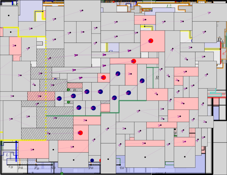
Figure 6: The left vertical edges (blue) and the right vertical edges (red) of an axis-parallel polygon. The polygon on the right is horizontally convex.

In order to describe our recursive partition, we initialize the corresponding tree $T$ with a root $r$ for which $P_{r}=S$. We define now a recursive procedure that takes as input a so far unprocessed vertex $v$ of the tree, corresponding to some polygon $P=P_{v}$. It either partitions $P$ further (hence adding children to $v$) or assigns at most one rectangle $R\in\mathrm{OPT}^{\prime}$ to $v$ and does not add children to $v$. We denote by $\mathrm{OPT}^{\prime}(P)\subseteq\mathrm{OPT}^{\prime}$ the subset of rectangles of $\mathrm{OPT}^{\prime}$ that are contained in $P$. If $\mathrm{OPT}^{\prime}(P)=\emptyset$, then we do not process $v$ further. If $|\mathrm{OPT}^{\prime}(P)|=1$, then we add the single rectangle in $\mathrm{OPT}^{\prime}(P)$ to $\mathcal{R}^{\prime}$, assign it to $v$, and do not process $v$ further. Assume now that $|\mathrm{OPT}^{\prime}(P)|>1$. We classify the vertical edges of $P$ as left vertical edges and right vertical edges (see Figure 6 in the appendix).

Definition 10.

For a vertical edge $e$ of an axis-parallel polygon $P$, we say that $e$ is left vertical if its interior contains a point $p=(p_{x},p_{y})$ such that the point $(p_{x}+\frac{1}{2},p_{y})$ is in $P$, and right vertical, otherwise.

For each point $p$ with integral coordinates on a left vertical edge of $P$, we define a line fence emerging from $p$, see Figure 3. If there is a point $p^{\prime}\in P$ such that (i) $p^{\prime}$ and $p$ have the same $y$-coordinate, (ii) the horizontal line segment connecting $p$ and $p^{\prime}$ intersects no rectangle of $\mathrm{OPT}^{\prime}(P)$ and (iii) $p^{\prime}$ is contained in the interior of the left side of a rectangle $R\in\mathrm{OPT}^{\prime}(P)$, or the top right corner or the bottom right corner of a rectangle $R\in\mathrm{OPT}^{\prime}(P)$, then we create a line fence that consists of the horizontal line segment from $p$ to $p^{\prime}$. Notice that if $p$ is contained in the interior of a left edge of a rectangle in $\mathrm{OPT}^{\prime}(P)$, then $p^{\prime}=p$ and the fence emerging from $p$ consists only of a single point. We call $p^{\prime}$ the endpoint of the fence emerging from $p$. We define line fences emerging at points of right vertical edges of $P$ in a symmetric manner. Denote by $F(P)$ the set of all fences created in this way.

When we partition $P$, we will cut $P$ along line segments such that (i) no horizontal line segment intersects a rectangle in $\mathrm{OPT}^{\prime}(P)$ and (ii) no interior of a vertical line segment intersects the interior of a line fence in $F(P)$. Intuitively, the line fences protect some rectangles in $\mathrm{OPT}^{\prime}(P)$ from being intersected by line segments defined in future iterations of the partition. This motivates the following definition.

Definition 11.

Given a horizontally convex polygon $P$, we say that a rectangle $R\in\mathrm{OPT}^{\prime}(P)$ is protected in $P$ if there exists a line fence $f\in F(P)$ such that the top edge or the bottom edge of $R$ is contained in $f$.

We will ensure that a protected rectangle will not be intersected when we cut $P$ by means of line fences in $F(P)$. We apply the following lemma to $P$.

Lemma 12 (Line-partitioning Lemma).

Given a horizontally convex (resp. vertically convex) polygon $P\in\mathcal{P}(26)$, such that $P$ contains at least two rectangles from $\mathrm{OPT}^{\prime}$, there exists a set $C$ of line segments with integral coordinates such that:

1. $C$ is composed of at most $8$ horizontal or vertical line segments that are all contained in $P$.

2. $P\setminus C$ has two or three connected components, and each of them is a horizontally (resp. vertically) convex polygon in $\mathcal{P}(26)$.

3. There is a vertical (resp. horizontal) line segment $\ell\in C$ such that $\ell$ intersects all the rectangles in $\mathrm{OPT}^{\prime}(P)$ that are intersected by $C$.

4. The line segment $\ell$ does not intersect any rectangle that is protected in $P$.

We introduce an (unprocessed) child vertex of $v$ corresponding to each connected component of $P\setminus C$ which completes the processing of $P$.

We apply the above procedure recursively to each unprocessed vertex $v$ of the tree until there are no more unprocessed vertices. Let $T$ denote the tree obtained at the end, and let $\mathcal{R}^{\prime}$ denote the set of all rectangles that we assigned to some leaf during the recursion. One can easily see that if a rectangle $R\in\mathrm{OPT}^{\prime}$ is protected in some polygon $P_{v}\supseteq R$ corresponding to a node $v\in T$, then $R$ will be protected in each polygon $P_{v^{\prime}}\subseteq P_{v}$ where $v^{\prime}$ is a descendant of $v$ in $T$. This implies that $R\in\mathcal{R}^{\prime}$.

3.2 Analysis

We want to prove that $|\mathcal{R}^{\prime}|\geq|\mathrm{OPT}|/6$. Consider an internal node $v$ of the tree and let $\ell_{v}$ be the corresponding line segment $\ell$ due to Lemma 12, defined above for partitioning $P_{v}$. We define a charging scheme for the rectangles in $\mathrm{OPT}^{\prime}$ that are intersected by $\ell_{v}$ and are not horizontally nested. For any such rectangle $R$, we will identify two rectangles $R_{L}$ and $R_{R}$ in $\mathrm{OPT}^{\prime}(P_{v})$ such that $R_{L}$ lies on the left of $R$ and $R_{R}$ lies on the right of $R$, and assign a charge of $1/2$ to each of them, and thus a total charge of $1$. More precisely, we will assign each of these charges to some corner of $R_{L}$ and $R_{R}$, respectively, and ensure that in the overall process each corner of each rectangle is charged at most once. Thus, each rectangle receives a total charge of at most $2$. Furthermore, if a rectangle receives a charge (to one of its corners), then it will be protected by the fences for the rest of the partitioning process.

One key difference to the algorithm of Mitchell [45] is that, in our algorithm, each application of Lemma 12 yields only one line segment $\ell$ that might intersect rectangles from $\mathrm{OPT}^{\prime}$. In the respective routine in [45] there can be two such line segments, and a consequence is that for each intersected rectangle $R\in\mathrm{OPT}^{\prime}$ there might be only one other rectangle from $\mathrm{OPT}^{\prime}$ to charge, rather than two. Furthermore, our proof of Lemma 12 is arguably simpler.

The charging scheme.

We now explain how to distribute the charge from rectangles that are intersected by $\ell_{v}$ (and are thus not in $\mathcal{R}^{\prime}$).

Definition 13.

We say that a rectangle $R\in\mathrm{OPT}^{\prime}$ sees the top-left corner $c$ of a rectangle $R^{\prime}\in\mathrm{OPT}^{\prime}$ on its right if there is a horizontal line segment $h$ that connects a point $p$ on the right edge of $R$ with $c$, such that $h$ does not intersect any rectangle in $\mathrm{OPT}^{\prime}$, $p$ is not the bottom-right corner of $R$, and $h$ does not contain the top edge of any other rectangle in ${R^{\prime\prime}\in}\mathrm{OPT}^{\prime}$.

Figure 4: Green marks indicate all the corners of the rectangles in $\mathrm{OPT}^{\prime}$ that are seen by the rectangle $R$. Corners displayed in red are examples of corners not seen by $R$. The one on the top is a bottom-left corner and here $p$ would be the top-right corner of $R$, which is excluded. The red corner on the right is not seen by $R$ because here $h$ would contain the top edge of $R^{\prime}$.

The last two conditions in the definition ensure that $R^{\prime}$ is not completely below $R$ (i.e., below the line that contains the bottom edge of $R$), and that $c^{\prime}$ is not “behind” $R^{\prime\prime}$. We define the bottom-left corner seen by $R\in\mathrm{OPT}^{\prime}$ on its right as well as the corners seen by $R\in\mathrm{OPT}^{\prime}$ on its left, top and bottom in a symmetric manner. See Figure 4.

It is easy to see that if a rectangle $R$ is horizontally nested, then there is at least one side (left or right) on which $R$ does not see any corner. On the other hand, if $R$ is not horizontally nested, then on its left it sees at least one corner of a rectangle in $\mathrm{OPT}^{\prime}(P)$, and similarly on its right. Intuitively, we will later charge $R$ to these rectangles in $\mathrm{OPT}^{\prime}(P)$.

Lemma 14.

Let $P$ be an axis-parallel polygon, and let $R$ be a rectangle in $\mathrm{OPT}^{\prime}(P)$ that is not protected in $P$ and not horizontally nested. Then, $R$ sees at least one corner of a rectangle in $\mathrm{OPT}^{\prime}(P)$ on its left, and at least one corner of another rectangle in $\mathrm{OPT}^{\prime}(P)$ on its right.

For every node $v\in T$ and every rectangle $R\in\mathrm{OPT}^{\prime}(P_{v})$ that is not horizontally nested and that is intersected by $\ell_{v}$, we assign a (fractional) charge of $1/2$ to a corner of a rectangle in $\mathrm{OPT}^{\prime}(P_{v})$ that $R$ sees on its left, and a charge of $1/2$ to a corner of a rectangle in $\mathrm{OPT}^{\prime}(P_{v})$ that $R$ sees on its right.

We prove now that if some rectangle $R\in\mathrm{OPT}^{\prime}$ is charged at some point, then $R\in\mathcal{R}^{\prime}$. The reason is that when $R$ is charged due to a vertical line segment $\ell_{v}$, then in the subsequent subproblems (i.e., corresponding to the children of $v$) $R$ will be protected.

Lemma 15.

If a rectangle $R^{\prime}\in\mathrm{OPT}^{\prime}$ receives a charge to at least one of its corner, then $R^{\prime}\in\mathcal{R}^{\prime}$.

In the next lemma, we show that each corner of a rectangle $R^{\prime}\in\mathcal{R}^{\prime}$ can be charged at most once. Hence, each rectangle receives a total fractional charge of at most 2.

Lemma 16.

Each corner of a rectangle in $\mathcal{R}^{\prime}$ is charged at most once.

As a consequence, each rectangle in $\mathcal{R}^{\prime}$ needs to pay for at most two other rectangles that are not horizontally nested and that were intersected, which loses a factor 3. We lose another factor 2 since we assumed that at most half of the rectangles in $\mathrm{OPT}^{\prime}$ are not horizontally nested. This yields a factor of 6 overall.

Lemma 17.

We have $|\mathcal{R}^{\prime}|\geq|\mathrm{OPT}|/6$.

3.2.1 Proof of the Line-partitioning Lemma

Now we prove Lemma 12. We assume w.l.o.g. that $P$ is horizontally convex with at most $26$ edges. We denote by $v\leq 13$ the number of vertical edges of $P$. We denote by $L(P)$ and $R(P)$ the set of the left and right vertical edges of $P$, respectively. Assume w.l.o.g. that $|L(P)|\geq|R(P)|$. Let $e_{1},...,e_{s}$ denote the left vertical edges of $P$, ordered from top to bottom. We have $s\geq v/2$. Consider the edges $E_{M}:=\{e_{\left\lfloor s/3\right\rfloor+1},...,e_{\left\lceil 2s/3\right\rceil}\}$, which are essentially the edges in the middle third of $e_{1},...,e_{s}$, see Figure 5. Let $f\in F(P)$ be a line fence in $F(P)$ emerging from a point $p$ on an edge in $E_{M}$ such that, among all such fences, its endpoint $p^{\prime}$ is the furthest to the right. Imagine that we define a vertical ray that emerges in $p^{\prime}$ and that is oriented downward. We follow this ray until we reach a point $q^{\prime}_{b}$ such that (i) $q^{\prime}_{b}$ is contained in the interior of the top edge of some rectangle $R_{b}\in\mathrm{OPT}^{\prime}(P)$ that is protected by some fence $g_{b}\in F(P)$, or (ii) $q^{\prime}_{b}$ is contained in some fence $g_{b}\in F(P)$ such that $q^{\prime}_{b}$ is neither the first nor the last point of $g_{b}$ (hence, intuitively $q^{\prime}_{b}$ is in the interior of $g_{b}$), or (iii) if we continued further we would leave $P$. In the first two cases, we define $q_{b}$ to be the point that $g_{b}$ emerges from, in the latter case we simply define $q_{b}:=q^{\prime}_{b}$. In a symmetric manner, we define a vertical ray that is oriented upward, emerging from $p^{\prime}$, and we define corresponding points $q_{t},q^{\prime}_{t}$, and possibly a corresponding fence $g_{t}\in F(P)$ and possibly a corresponding rectangle $R_{t}\in\mathrm{OPT}^{\prime}(P)$.

We define $C_{b}$ to be a sequence of line segments that connect $p$ with $q_{b}$, using only points in $f$, $\overline{p^{\prime}q^{\prime}_{b}}$, the top edge of $R_{b}$, the left edge of $R_{b}$ and $g_{b}$, see Figure 5. We define $C_{t}$ similarly. Then we define our cut $C$ by $C:=C_{b}\cup C_{t}$ with $\ell:=\overline{q_{t}^{\prime}q^{\prime}_{b}}$. Note that $C$ has at most 8 edges. By construction, $\ell$ is the only line segment in $C$ that can intersect rectangles in $\mathrm{OPT}^{\prime}$, however, $\ell$ does not intersect any protected rectangle. Also, the length of $\ell$ is strictly larger than zero.

We need to argue that each connected component of $P\setminus C$ has at most 26 edges, i.e., at most $13$ vertical edges. First, $P\setminus C$ consists of at most three connected components: apart from the boundary of $P$, the first component $P_{1}$ is enclosed by $C_{t}$, the second component $P_{2}$ is enclosed by $C_{b}$ and the last component $P_{3}$ is enclosed by the sequence of line segments $C_{r}\subseteq C$ that connects $q_{t}$ and $q_{b}$. Now observe that the boundary of $P_{1}$ is disjoint from the edges $E_{B}:=\{e_{\left\lceil 2s/3\right\rceil+1},\dots,e_{s}\}$, the boundary of $P_{2}$ is disjoint from $E_{T}:=\{e_{1},\dots,e_{\left\lfloor s/3\right\rfloor}\}$, and the boundary of $P_{3}$ is disjoint from $E_{M}$. Since $C_{b}$ (and $C_{t}$) has at least $\lfloor s/3\rfloor\geq\lfloor v/6\rfloor$ vertical edges, and $C_{b}$ (and $C_{t}$) has at most $2$ vertical edges, the number of vertical edges of $P_{1}$ (and $P_{2}$) is at most $v-\lfloor v/6\rfloor+2=\lceil\frac{5}{6}v\rceil+2\leq\lceil\frac{5}{6}\cdot 13\rceil+2=13$. Similarly, since $E_{M}$ has at least $\lceil s/3\rceil\geq\lceil v/6\rceil$ vertical edges and $C_{r}$ has at most $3$ vertical edges, the number of vertical edges of $P_{3}$ is at most $v-\lceil v/6\rceil+3=\lfloor\frac{5}{6}v\rfloor+3\leq\lfloor\frac{5}{6}\cdot 13\rfloor+3=13$.

Finally, we would like $P\setminus C$ to have at least two connected components. This is clearly true if $\ell$ or $\overline{pp^{\prime}}$ contain a point in the interior of $P$. One can show that if this is not the case, then $\overline{pp^{\prime}}$ must be identical with the top or the bottom edge of $P$ and $p^{\prime}$ must be the top-right corner of a rectangle $R\in\mathrm{OPT}^{\prime}(P)$ (see Figure 5), we refer to Appendix C.10 for details. Due to our choice of $f$ this implies that $\left\lfloor s/3\right\rfloor+1=1$ and hence $P$ has at most $4s\leq 8$ edges. Thus, we can for example define a cut $C^{\prime}$ that consists of the horizontal line segment between $p$ and the top-left corner of $R$, the left edge of $R$, and the bottom edge of $R$.

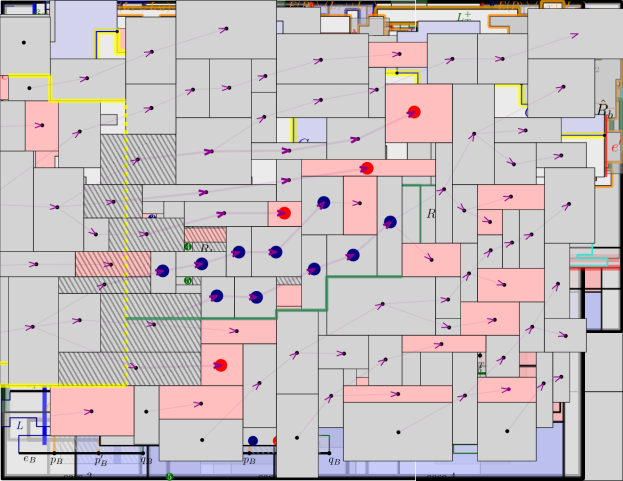
Figure 5: Partitioning an horizontally convex polygon with $26$ edges (left). If the partitioning process fails to create two connected components, the polygon must have at most 8 edges (right). In both cases, the set of line segments $C$ used to cut the polygon is shown in yellow.

4 Improving the approximation ratio to 3

In this section, we give an overview of our additional ideas to obtain an approximation ratio of 3; we refer to Appendix A for details. One key idea is to use more elaborate fences that are no longer just horizontal line segments, but instead $x$-monotone sequences of $\tau=O(1)$ line segments, see Figure 7 in Appendix. Like before, each of them emerges on a point of some vertical edges of the corresponding polygon $P$. We refer to these new fences as $\tau$-fences and hence our previous fences are 1-fences. In particular, $\tau$-fences protect more rectangles from $\mathrm{OPT}$ (if $\tau$ is sufficiently large), see Figure 7.

One benefit of these larger fences is the following. Suppose that we apply a cut $C$ to a polygon $P$, let $\ell$ denote the single (vertical) line segment in $C$ that intersects rectangles from $\mathrm{OPT}^{\prime}$. Assume that due to $C$, the top-right or bottom-right corner of some rectangle $R$ is charged. In the argumentation in Section 3.1, it could happen that later the top-left or bottom-left corner of $R$ is charged by some rectangle $R^{\prime}$. However, if we use $\tau$-fences for some $\tau\geq 3$, then after applying the cut $C$, such a rectangle $R^{\prime}$ is protected by a $\tau$-fence that emerges from a point on $\ell$ (which is a vertical edge in the connected component of $P\setminus C$ that contains $R$). Therefore, at most two corners from each rectangle receive a charge: either only its left or only its right corners. Therefore, each rectangle $R\in\mathcal{R}^{\prime}$ receives a fractional charge of at most 1. Thus, due to this we lose only a factor of 2, in addition to the factor of 2 that we lost by assuming that there are at most $|\mathrm{OPT}|/2$ horizontally nested rectangles (and we assumed that we lost them completely). Hence, already this improves the approximation ratio to 4.

Then, we improve the approximation ratio to 3 with the following argumentation. Suppose that a rectangle $R\in\mathrm{OPT}^{\prime}$ is intersected by some cut $C$ such that $R$ is not horizontally nested. If $R$ sees two corners of (one or two) other rectangles in $\mathrm{OPT}^{\prime}$ on its right, then we can charge $R$ to these two corners, instead of charging it only to one corner like in the argumentation above. If we can do this for all intersected rectangles $R\in\mathrm{OPT}^{\prime}$ (towards their respective left and right), then one can show that this already improves the approximation ratio to 3. However, it might be that $R$ sees only one such corner $c$ on its right. Then we show that one of the following two cases applies. The first case is that we identify two corners $c^{\prime},c^{\prime\prime}$ belonging to rectangles $R^{\prime},R^{\prime\prime}$ on the right of $R$ such that $R$ sees $c^{\prime}$ but $R$ does not see $c^{\prime\prime}$. However, we show that if $\tau\geq 7$ then this ensures that $R^{\prime\prime}\in\mathcal{R}^{\prime}$, that $c^{\prime\prime}$ will not be charged again if $R^{\prime\prime}$ is not horizontally nested and at most twice in total otherwise, and that the corners of $R^{\prime\prime}$ on the opposite side will never be charged. Hence, we can assign a charge of $1/4$ each to $c^{\prime}$ and $c^{\prime\prime}$. The second case is that $R$ sees a corner $\hat{c}$ of a horizontally nested rectangle $\hat{R}$ on the right of $R$. In this case, we assign a charge of $1/2$ to $\hat{c}$. One may wonder why we can afford to assign a charge of $1/2$ to $\hat{c}$ (and similarly before two charges of $1/4$ each to $c^{\prime\prime}$ if $R^{\prime\prime}$ is horizontally nested). The intuitive reason is that we had already given up on the horizontally nested rectangles, assuming a loss of a factor of 2. However, after charging $\hat{c}$ we ensure that $\hat{R}\in\mathcal{R}^{\prime}$ (we show that $\tau\geq 3$ suffices) while we had assumed that we had already lost $\hat{R}$. Hence, we can assign a charge of 1 unit to $\hat{R}$ “for free”.

We choose $\tau:=7$ and hence we need a recursive partitioning scheme that does not cut through any ${7}$-fence. In fact, we prove even a stronger statement that could be useful for future work: we show that for any constant $\tau\in\mathbb{N}$ there is a recursive partitioning scheme into polygons in $\mathcal{P}(30\tau+18)$ such that each recursive cut does not cut through any $\tau$-fence. In particular, our routine for cutting one given polygon is a generalization of Lemma 12. The resulting polygons might no longer be horizontally convex; we allow them to be arbitrary simple axis-parallel polygons with $O(\tau)$ vertices and integral coordinates. However, we can still establish the necessary partitioning scheme via distinguishing only a few different cases.

See 1

Appendix A A recursive partitioning for a 3-approximate set

In this section, we construct a $228$-recursive partition for a set $\mathcal{R}^{\prime}\subseteq\mathrm{OPT}^{\prime}$, such that $|\mathcal{R}^{\prime}|\geq\frac{1}{3}|\mathrm{OPT}^{\prime}|$, where $\mathrm{OPT}^{\prime}$ denotes the set of maximal rectangles in $S$. We first show how to construct this recursive partition to obtain $\mathcal{R}^{\prime}$, using a more general Partitioning Lemma (Lemma 20) than for the $6$-approximation. Then, we prove the Partitioning Lemma, and finally we describe a charging scheme for the rectangles that are intersected during the partitioning process, and analyze it to show that $\mathcal{R}^{\prime}$ is a $3$-approximate solution.

A.1 Recursive Partitioning

As before, we assume without loss of generality that at most half of the rectangles in $\mathrm{OPT}^{\prime}$ are horizontally nested. Otherwise, it must be that at most half of the rectangles in $\mathrm{OPT}^{\prime}$ are vertically nested, and we can for example rotate $\mathrm{OPT}^{\prime}$ by $90$ degrees to obtain an equivalent instance $\mathrm{OPT}^{\prime}$ where at most half of the rectangles are horizontally nested.

In order to describe this recursive partition, we initialize the corresponding tree $T$ with root $r$. We define now a recursive procedure that takes as input a so far unprocessed vertex $v$ of the tree, corresponding to some polygon $P=P_{v}$. It either partitions $P$ further (hence adding children to $v$) or assigns a rectangle $R\in\mathrm{OPT}^{\prime}$ to $v$ and does not add children to $v$. We denote by $\mathrm{OPT}^{\prime}(P)\subseteq\mathrm{OPT}^{\prime}$ the subset of rectangles of $\mathrm{OPT}^{\prime}$ that are contained in $P$. If $\mathrm{OPT}^{\prime}(P)=\emptyset$, then we simply delete $v$ from $T$. If $|\mathrm{OPT}^{\prime}(P)|=1$ then we add the single rectangle in $\mathrm{OPT}^{\prime}(P)$ to $\mathcal{R}^{\prime}$, assign it to $v$, and do not process $v$ further.

Assume now that $|\mathrm{OPT}^{\prime}(P)|>1$.

Figure 7: Some $5$-fences emerging from a left vertical edge (blue) on the boundary of an axis-parallel polygon. Shaded rectangles are the rectangles in $\mathrm{OPT}^{\prime}$ that intersect the boundary of $P$. White spaces indicate points that are not covered by rectangles of $\mathrm{OPT}^{\prime}$ contained in $P$. Darker gray rectangles correspond to rectangles in $\mathrm{OPT}^{\prime}(P)$ that are $5$-protected.

We say that a curve $\gamma$ of the plane is $x$-monotone (resp. $y$-monotone) if for any vertical (resp. horizontal) line $\ell$, the intersection $\ell\cap\gamma$ is connected.

Given an integral parameter $\tau\geq 1$ and a vertical edge $e$ of $P$, a $\tau$-fence anchored on $e$ is a $x$-monotone curve defined by a sequence of at most $\tau$ horizontal and vertical line segments that is contained in $P$, has one endpoint on $e$ and intersects no rectangles of $\mathrm{OPT}^{\prime}$. See Figure 7. Denote by $F_{\tau}(P)$ the set of all fences created in this way.

When we partition $P$, we will cut $P$ along a sequence of line segments such that (i) no horizontal line segment intersects a rectangle in $\mathrm{OPT}^{\prime}(P)$ and (ii) the interior of any line segment is disjoint from the interior of any $\tau$-fence. Therefore, the $\tau$-fences intuitively protect some rectangles in $\mathrm{OPT}^{\prime}(P)$ from being intersected by line segments defined in future iterations of the partition. This motivates the following definition.

Definition 18.

Given a polygon $P$, we say that a rectangle $R\in\mathrm{OPT}^{\prime}(P)$ is $\tau$-protected in $P$ if there exists a vertical edge $e$ in $P$ such that the top side of $R$ is contained in a $\tau$-fence emerging from $e$ and the bottom of $R$ is contained in another $\tau$-fence also emerging from $e$.

Observation 19.

Given an axis-parallel polygon $P$ and a parameter $\tau\geq 3$, if a rectangle $R\in\mathrm{OPT}^{\prime}(P)$ has its top or bottom edge contained in a $(\tau-2)$-fence, then it is $\tau$-protected.

Proof.

Without loss of generality, we assume that the top edge of $R$ is contained in a $(\tau-2)$-fence $f$ anchored on a point $p$ on a left vertical edge of $P$. Using $f$, the left edge of $R$ and the bottom edge of $R$, we can construct another fence an $x$-monotone sequence of at most $\tau$ line segments anchored on $p$ that contains the bottom edge of $R$. Thus, $R$ is $\tau$-protected. ∎

We will ensure that no protected rectangle will be intersected when we cut $P$, and the fences in $F_{\tau}(P)$ will help us to ensure this. We apply the following lemma to $P$ with $\tau=7$.

Lemma 20 (Partitioning Lemma).

Let $\tau\geq 1$ be an integer. Let $P$ be a simple axis-parallel polygon with at most $30\tau+18$ edges of integral coordinates, such that $P$ contains at least two rectangles from $\mathrm{OPT}^{\prime}$. Then there exists a sequence $C$ of line segments with integral coordinates such that:

1. $C$ is composed of at most $2\tau+1$ horizontal or vertical line segments that are all contained in $P$.

2. $P\setminus C$ has exactly two connected components, and each of them is a simple axis-parallel polygon with at most $30\tau+18$ edges.

3. There is a vertical line segment $\ell$ of $C$ that intersects all the rectangles in $\mathrm{OPT}^{\prime}(P)$ that are intersected by $C$.

4. $\ell$ does not intersect any rectangle that is $\tau$-protected in $P$.

We introduce an (unprocessed) child vertex of $v$ corresponding to each connected component of $P\setminus C$ which completes the processing of $P$.

We apply the above procedure recursively to each unprocessed vertex $v$ of the tree until there are no more unprocessed vertices. Let $T$ denote the tree obtained at the end, and let $\mathcal{R}^{\prime}$ denote the set of all rectangles that we assigned to some leaf during the recursion.

Lemma 21.

The tree $T$ and the set $\mathcal{R}^{\prime}$ satisfy the following properties.

1. For each node $v\in T$, the horizontal edges of $P_{v}$ do not intersect any rectangle in $\mathrm{OPT}^{\prime}$.

2. $T$ is a $228$-recursive partition for $\mathcal{R}^{\prime}$.

3. If a rectangle $R\in\mathrm{OPT}^{\prime}$ is $7$-protected in $P_{v}$ for some node $v\in T$, then

   • it is $7$-protected in $P_{v^{\prime}}$ for each descendant $v^{\prime}$ of $v$,

   • $R\in\mathcal{R}^{\prime}$.

Proof.

The first and second properties follow from the definition of the fences and Lemma 20. The third property follows from the fact that for any $\tau\geq 1$, if $f$ is a $\tau$-fence in $F(P_{v})$ then, $f\cap P_{v^{\prime}}$ is a $\tau$-fence of $F(P_{v^{\prime}})$. ∎

A.2 Proof of the Partitioning Lemma

In this section, we prove the partitioning Lemma used to construct the recursive partitioning of $S$. First, given an axis-parallel polygon $P$ with $k$ edges (and with no holes), we label the edges of $P$ according to their order in the boundary starting from an arbitrary edge in a clockwise fashion: $E(P)=e_{1},\dots,e_{k}$. The distance between two edges $e_{i}$ and $e_{j}$ with $i\leq j$ is $d(e_{i},e_{j})=\min\{j-i,k-j+i\}$.

We will start by proving the following helpful lemma, which establishes a similar result as the one from Chazelle ([20], Theorem 2) but now in the context of axis-parallel polygons.

Lemma 22.

Given an axis-parallel polygon $P$ with $k$ edges, there exists a vertical line segment $\ell$ such that $\ell$ is contained in $P$ and its endpoints are respectively contained in two horizontal edges of distance at least $k/3$.

Proof.

Let $\mathcal{L}$ be the set of vertical line segments contained in $P$ and with both endpoints on $P$’s boundary. Notice that a vertical line segment $\ell\in\mathcal{L}$ may contain some of $P$’s vertical edges. We also denote by $e_{T}$ and $e_{B}$ the horizontal edges of $P$ in which the top and the bottom endpoint of $\ell$ are respectively contained. Finally we denote $d(\ell):=d(e_{B},e_{T})$.

To prove the lemma, we must show that there exists $\ell\in\mathcal{L}$ such that $d(\ell)\geq k/3$. For this, consider any $\ell\in\mathcal{L}$ such that $d(\ell)<k/3$. We construct, via a complete case analysis, another $\ell^{\prime}\in\mathcal{L}$ such that $d(\ell^{\prime})>d(\ell)$. See Figure 8.

Figure 8: Different cases in the proof of Lemma 22. The line $\ell\in\mathcal{L}$ is displayed in orange, between points $p_{B}$ and $p_{T}$. On the polygon, edges from $L$ are shown in blue, while edges in $R$ are shown in green. The cut $\ell^{\prime}$ such that $d(\ell^{\prime})>d(\ell)$ is shown with a dashed thick red line.

We orient the edges of $P$ in a clockwise fashion. In this order, we can partition $P$’s boundary as: $E(P)=e_{B}\cup L\cup e_{T}\cup R$. W.l.o.g. we assume that $|R|\geq|L|$. In particular, we have $d(\ell)=|L|+1$.

Let $p_{T}=\ell\cap e_{T}$ and $p_{B}=\ell\cap e_{B}$ denote the top and bottom endpoint of $\ell$ respectively. Similarly as the left and right vertical edges, we define the top horizontal edges (resp. bottom horizontal edges) of $P$ to any horizontal edge $e$, that contains in its interior a point $(x,y)$ such that the point $(x,y-1/2)\in P$ (resp. $(x,y+1/2)\in P$).

1. If $e_{T}$ is a bottom horizontal edge of $P$, then since $\ell$ is contained in $P$, $p_{T}$ must be an endpoint of $e_{T}$.

   1. If $p_{T}$ is the left endpoint of $e_{T}$, then $p_{T}$ must be the top endpoint of an vertical edge $e^{\prime}$ of $P$. Furthermore, $e^{\prime}$ is strictly contained in $\ell$, i.e., the bottom endpoint $q$ of $e^{\prime}$ is contained in $\ell$ strictly above $p_{B}$. The vertex $q$ is contained in a horizontal edge $e\in R$ and we have $d(e_{B},e)=d(e_{B},e_{T})+2$. Thus, the vertical line segment $\ell^{\prime}$ with endpoints $p_{B}$ and $q$ is in $\mathcal{L}$ and we have $d(\ell^{\prime})=d(\ell)+2$.

   2. Otherwise, $p_{T}$ is the right endpoint of $e_{T}$. In this case, let $q$ be the lowest point above $p_{T}$, with the same $x$-coordinate as $p_{T}$ that is contained in the boundary of $P$. The point $q$ lies in a horizontal edge $e\in R$. We claim that either $d(e_{B},e)$ or $d(e,e_{T})$ is greater than $d(e_{B},e_{T})$. For the sake of a contradiction, assume that both are smaller than or equal to $d(\ell)$. Then, it must be that $d(e_{B},e_{T})+d(e_{T},e)+d(e,e_{B})=k$, which implies that $d(e_{B},e_{T})\geq k/3$. Thus, we have either $d(e_{T},e)>d(\ell)$ — in which case we define $\ell^{\prime}$ as the vertical line segment with endpoints $q$ and $p_{T}$ — or $d(e_{B},e)>d(\ell)$, and we then define $\ell^{\prime}$ as the vertical line segment with endpoints $q$ and $p_{B}$. In both cases, we have $\ell^{\prime}\in\mathcal{L}$ and $d(\ell^{\prime})>d(\ell)$.

2. If $e_{B}$ is a top horizontal edge of $P$, then we proceed symmetrically as case 1 to obtain $\ell^{\prime}\in\mathcal{L}$ such that $d(\ell^{\prime})>d(\ell)$.

Otherwise, $e_{T}$ is a top horizontal edge and $e_{B}$ is a bottom horizontal edge. Let $q_{T}$ and $q_{B}$ denote the right endpoint of $e_{T}$ and the right endpoint of $e_{B}$, respectively.

1. If $p_{T}=q_{T}$, then $q_{T}$ must be the top endpoint (or the bottom) of a vertical edge $e^{\prime}$ of $P$. The other endpoint $q$ of $e^{\prime}$ is contained in a horizontal edge $e\in R$. Let $\ell^{\prime}$ be the vertical line segment joining $p_{B}$ and $q$. It is clear that $\ell^{\prime}$ is in $\mathcal{L}$ and since $e\in R$, we have $d(\ell^{\prime})=d(\ell)+2$.

2. If $p_{B}=q_{B}$, then we proceed symmetrically as case 2 to obtain $\ell^{\prime}\in\mathcal{L}$ such that $d(\ell^{\prime})=d(\ell)+2$.

Otherwise, both $q_{T}$ and $q_{B}$ are strictly on the right of $\ell$. W.l.o.g. we assume that $q_{T}$ has $x$-coordinate smaller than or equal to the one of $q_{B}$. Now, define the closed rectangular area $W$ that has $\ell$ as left side and $q_{T}$ as top-right corner.

1. If $W$ intersects no horizontal edge $e\in R$, then in particular the right side of $W$ is contained in $P$. Let $p^{\prime}_{B}$ denote the bottom-right corner of $W$. By assumption, $p^{\prime}_{B}$ lies in $e_{B}$. We replace $\ell$ by the vertical line segment $\hat{\ell}$ between $q_{T}$ and $p^{\prime}_{B}$. We have $\hat{\ell}\in\mathcal{L}$, and $d(\hat{\ell})=d(\ell)$. Then, $\hat{\ell}$ satisfies the requirements of case 2. We apply the same process as in case 2 to obtain $\ell^{\prime}\in\mathcal{L}$ such that $d(\ell^{\prime})=d(\hat{\ell})+2=d(\ell)+2$.

2. Otherwise, $W$ intersects some horizontal edge in $R$. Since $\ell$ is contained in $P$, each such horizontal edge must have its left endpoint in $W$. Let $q\in W$ be (any of) the leftmost left endpoint of a horizontal edge $e\in R$. The vertical line segment between $e_{B}$ and $e_{T}$ that passes by $q$ is contained in $P$: by the choice of $q$, it does not intersect the interior of any horizontal edge in $R$, and since $\ell\subset P$, no horizontal edge in $L$ intersects the interior of $W$. Then, since $e\in R$, we can apply the same argumentation as in case 1(b) and prove that either $d(e_{B},e)$ or $d(e_{B},e)$ is greater than $d(e_{B},e_{T})=d(\ell)$. If $d(e_{T},e)>d(e_{B},e_{T})$, we define $\ell^{\prime}$ to be the vertical line segment between $e_{B}$ and $q$. Otherwise, we define $\ell^{\prime}$ to be the vertical line segment between $e_{T}$ and $q$. In both cases, $\ell^{\prime}\in\mathcal{L}$ and $d(\ell^{\prime})>d(\ell)$.

Thus, for any $\ell\in\mathcal{L}$ such that $d(\ell)<k/3$, we have constructed another line $\ell^{\prime}\in\mathcal{L}$ such that $d(\ell^{\prime})>d(\ell)$. Consequently, the element $\ell_{0}\in\mathcal{L}$ that maximizes $d(\ell)$ over all $\ell\in\mathcal{L}$ must satisfy $d(\ell_{0})\geq k/3$. ∎

We can now prove our Partitioning Lemma restated below.

See 20

Proof.

Let $P$ be an axis-parallel polygon with $k\leq 30\tau+18=15(2\tau+1)+3$ edges.

1. If $k\leq 15(2\tau+1)-1$, then let $R$ be one of the rectangles of $\mathrm{OPT}^{\prime}(P)$ with the leftmost left side. The leftward horizontal ray $h_{T}$ (resp. $h_{B}$) from the top-right corner of $R$ (resp. from the bottom-right corner of $R$) reaches $P$’s boundary without intersecting any rectangle in $\mathrm{OPT}^{\prime}(P)$. Let $C$ be the union of $h_{T}$, $h_{B}$, and the right side of $R$. The cut $C$ intersects no rectangles in $OPT^{\prime}(P)$ and $P\setminus C$ has at least two connected components. Since $C$ has three line segments, each of these component has at most $15(2\tau+1)-1+3+1=15(2\tau+1)+3$ edges.

We assume now that $P$ has $k\geq 15(2\tau+1)$ edges. To construct a cut $C$ we will identify two $\tau$-fences $f_{1}$ and $f_{2}$ in $P$, and one vertical line segment $\ell$ that connects two points on $f_{1}$ and $f_{2}$ (with integral coordinates), and does not intersect the interior of any other $\tau$-fences. In particular, no $\tau$-protected rectangle is intersected by $\ell$. We will define the cut $C$ as a subset of $f_{1}\cup\ell\cup f_{2}$, so in particular it will consists of at most $2\tau+1$ line segments. We will choose $f_{1}$ and $f_{2}$ so that they are respectively anchored on vertical edges of distance at least $2\tau+2$ from each other. This implies that each of the two connected components of $P\setminus C$ will have at most $k\leq 30\tau+18$ edges.

In some degenerate cases, the connected components of $P\setminus C$ may not be simple axis-parallel polygons. More precisely, each connected component may have some vertical edges that intersect and some horizontal edges that intersect, but since $C$ is contained in $P$ no vertical edge can cross an horizontal edge. This is due to the fact that $\tau$-fences may contain some edges of the polygon, and thus, the cut $C$ may intersect $P$’s boundary not only on its endpoints. See Figure 10. If this is the case, we will argue at the end of the proof that there exists a subset $C^{\prime}\subset C$ that intersects $P$’s boundary only on its endpoints, and so that $P\setminus C^{\prime}$ has exactly two connected components that are simple axis-parallel polygon with at most $k\leq 30\tau+18$ edges.

Let $\ell_{0}$ be the vertical line segment given by Lemma 22. Recall that the edges of $P$ are ordered in a clockwise fashion. In this order, we have: $E(P)=e_{B}\cup L\cup e_{T}\cup R$. By the choice of $\ell_{0}$ we know that both $L$ and $R$ have size at least $k/3-1\geq 5(2\tau+1)-1$. Since $|L|$ and $|R|$ are odd numbers, we have $|L|\geq 5(2\tau+1)$ and $|R|\geq 5(2\tau+1)$. We further partition each of these groups into three subgroups according to the clockwise ordering: $L=L_{B}\cup L_{M}\cup L_{T}$ and $R=R_{T}\cup R_{M}\cup R_{B}$ (See Figure 9), such that

• The middle-left group $L_{M}$ and the middle-right group $R_{M}$ contain each at least $2\tau+1$ edges.

• The bottom-left group $L_{B}$, the top-left group $L_{T}$, the bottom-right group $R_{B}$ and the top-right group $R_{T}$ contain at least $2(2\tau+1)$ edges each.

Figure 9: The partition of $P$’s boundary into sets $\{e_{B}\},L_{B},L_{M},L_{T},\{e_{T}\},R_{T},R_{M},R_{B}$. Middle groups $L_{M}$ and $R_{M}$ each contains at least $2\tau+1$ edges, while other groups ($L_{T},L_{B},R_{B}$ and $R_{T}$) each contains at least $2(2\tau+1)$ edges.

Let $p_{1},p_{2},\dots,p_{r}$ the set of points of $\ell_{0}$, ordered from bottom to top, such that each $p_{i}$, $i\in[r]$ is contained in a $\tau$-fence. Let $E_{i}$ be the set of vertical edges $e$ such that there exists a $\tau$-fence anchored in $e$ that contains $p_{i}$. Finally, we define $J=\cup_{i=1}^{r}E_{i}$.

Remark. Notice that the edge $e_{B}$ is covered by two $1$-fences $f$ and $f^{\prime}$ (that are also $\tau$-fences), such that $f$ (resp. $f^{\prime}$) is anchored on the vertical $e\in L_{B}$ (resp. $e^{\prime}\in R_{B}$) that is incident to $e_{B}$. In particular, we have that $p_{1}\in e_{B}$, $E_{1}\cap L_{B}\neq\emptyset$ and $E_{1}\cap R_{B}\neq\emptyset$. Similarly, we remark that $p_{r}\in e_{T}$, $E_{r}\cap L_{T}\neq\emptyset$ and $E_{r}\cap R_{T}\neq\emptyset$.

1. First assume that $(L_{M}\cup R_{M})\cap J=\emptyset$, i.e., none of the fences anchored on edges in $L_{M}\cup R_{M}$ intersects $J$. We define $B=R_{B}\cup e_{B}\cup L_{B}$ and $T=L_{T}\cup e_{T}\cup R_{T}$. For any edges $e\in B$ and $e^{\prime}\in T$, we have $d(e,e^{\prime})\geq\min(|L_{M}|,|R_{M}|)+1\geq 2\tau+2$.

   1. If there is an index $i$ such that $E_{i}\cap B\neq\emptyset$ and $E_{i}\cap T\neq\emptyset$ then it means that $p_{i}$ is contained in a fence $f$ anchored on a edge $e$ of $B$ and $p_{i}$ is also contained in one fence $f^{\prime}$ anchored on an edge $e^{\prime}$ of $T$. Thus, there exists a cut $C\subseteq f\cup f^{\prime}\subset P$ that is a sequence of at most $|f|+|f^{\prime}|\leq 2\tau$ line segments, that connects two points of the boundary contained on edges at distance at least $2\tau+2$ from each other. Thus, each connected components of $P\setminus C$ has at most $k-1\leq 15(2\tau+1)+2$ edges. Since $C$ is a subset of two fences, it does not intersect any rectangle in $\mathrm{OPT}^{\prime}(P)$.

   2. If there is no such index, then each $E_{i}$ is either contained in $B$ or in $T$. In particular we obtain that $E_{1}\subseteq B$ and $E_{r}\subseteq T$. Thus, there exists $1\leq i\leq r-1$ such that $E_{i}\subseteq B$ and $E_{i+1}\subseteq T$. Thus, let $\ell$ be the vertical line segment between $p_{i}$ and $p_{i+1}$. The point $p_{i}$ is contained in a fence $f$ anchored on a edge $e\in B$ and $p_{i+1}$ is contained in a fence $f^{\prime}$ anchored on an edge $e^{\prime}\in T$. In particular, we have $d(e,e^{\prime})\geq 2\tau+1$. Thus, there exists a sequence $C\subseteq f\cup\ell\cup f^{\prime}$ of at most $2\tau+1$ line segments that connects $e$ and $e^{\prime}$, and since $d(e,e^{\prime})\geq 2\tau+1$, each component of $P\setminus C$ has at most $k\leq 15(2\tau+1)+3$ edges.

      We now check that conditions (3) and (4) hold. Since $f$ and $f^{\prime}$ are $\tau$-fences, it is clear that only $\ell$ may intersect some rectangles in $\mathrm{OPT}^{\prime}(P)$. Then, for the sake of a contradiction, assume that $\ell$ intersects a rectangle $R\in\mathrm{OPT}^{\prime}(P)$ that is $\tau$-protected. There exists two $\tau$-fences $g$ and $g^{\prime}$, both anchored on the same edge $e^{\prime\prime}$, such that the top edge of $R$ is contained in $g$ and the bottom side of $R$ is contained in $g^{\prime}$. Since $\ell$ intersects $R$, it must intersect the interior of $g$ and $g^{\prime}$. This implies that $p_{i}\in g^{\prime}\cap\ell$ and $p_{i+1}\in g\cap\ell$, and in particular we have $e^{\prime\prime}\in E_{i}\cap E_{i+1}$ and also $e^{\prime\prime}\notin(L_{M}\cup R_{M})$. Thus, $e^{\prime\prime}\in T\cup B$, which brings a contradiction with the fact that $E_{i}\subseteq B$ and $E_{i+1}\subseteq T$. Therefore, $C$ does not intersect any $\tau$-protected rectangle.

2. Now consider now the case $L_{M}\cap J\neq\emptyset$ or $R_{M}\cap J\neq\emptyset$; by symmetry, we can assume that $L_{M}\cap J\neq\emptyset$. Let $f$ be the fence anchored on an edge $e\in L_{M}$, with the rightmost endpoint $p$ among all $\tau$-fences anchored on $L_{M}$. In particular, $f$ must intersect $\ell_{0}$. Let $q$ denote the lowest point on the upward vertical ray starting from $p$, such that $q$ is contained in the interior of a $\tau$-fence $g$. We denote $e_{g}$ the edge on which $g$ is anchored. We also denote $\ell$ the vertical line segment between $p$ and $q$ (we may have $q=p$). Similarly, let $\hat{q}$ denote the highest point on the downward vertical ray $\hat{\ell}$ from $p$, such that $\hat{q}$ is contained in the interior of a $\tau$-fence $\hat{g}$ anchored on an edge $e_{\hat{g}}$ (we may also have $\hat{q}=p$). By the choice of $f$, we know that both $e_{g}$ and $e_{\hat{g}}$ are not in $L_{M}$.

   

   1. If $e_{g}\in R$, then the distance between $e$ and $e_{g}$ is at least $\min(|L_{T}|,|L_{B}|)+1\geq 2\tau+2$. Thus, there exists a cut $C\subseteq f\cup\ell\cup g$ with at most $2\tau+1$ line segments, that satisfies the properties (1)-(3) of the Partitioning Lemma. To prove that the last property also holds, we can use a similar argumentation as in case 1(b). Here, assuming that $\ell$ intersects a $\tau$-protected rectangle would imply a contradiction with the definition of $q$ as the lowest point above $p$ that is contained in the interior of a $\tau$-fence.

   2. Similarly, if $e_{\hat{g}}\in R$, then we can define a cut $C\subseteq f\cup\hat{\ell}\cup\hat{g}$.

   3. Consider now the case where both $e_{g}$ and $e_{\hat{g}}$ are in $L$. Recall that, by definition of $f$, we know that $e_{g}$ and $e_{\hat{g}}$ are not in $L_{M}$.

      

      1. If $e_{\hat{g}}\in L_{B}$ and $e_{g}\in L_{T}$ then $d(e_{\hat{g}},e_{g})\geq\min(|L_{M}|,|R|)+1\geq 2\tau+2$, and we define $C\subseteq g\cup\ell\cup\hat{\ell}\cup\hat{g}$.

      2. If $e_{\hat{g}}\in L_{T}$ and $e_{g}\in L_{B}$ then we also have $d(e_{\hat{g}},e_{g})\geq\min(|L_{M}|,|R|)\geq 2\tau+2$. In this case, $g$ and $\hat{g}$ must intersect and thus $C$ consists of the proper subset of $g\cup\hat{g}$ that connects $e_{g}$ and $e_{\hat{g}}$.

      3. In the remaining case, $e_{g}$ and $e_{\hat{g}}$ are both in $L_{T}$ or both in $L_{B}$. These two cases are symmetrical so we only describe how to proceed in the former case. Let $\ell^{\prime}$ denote the downward vertical ray from $f$’s endpoint $p$ to a point $q^{\prime}$ on the boundary of $P$. Let $q^{\prime}_{1},\dots,q^{\prime}_{r^{\prime}}$ be the points on $\ell^{\prime}$, from top to bottom, such that each $q^{\prime}_{i}$ is contained in the interior of a $\tau$-fence. Let $E^{\prime}_{1},\dots,E^{\prime}_{r^{\prime}}$ be sets of edges from $P$ such that $e^{\prime}\in E^{\prime}_{i}$ if there exists a fence anchored in $e^{\prime}$ that contains $q^{\prime}_{i}$. We know that $E^{\prime}_{r^{\prime}}\cap(R\cup\{e_{B}\})\neq\emptyset$, and by definition of $f$ we also have that, for all $i\geq 1$, $E^{\prime}_{i}\cap L_{M}=\emptyset$.

         We know that $q^{\prime}$ lies on an horizontal edge contained in $R\cup\{e_{B}\}\subset E(P)\setminus(L_{T}\cup L_{M})$. Additionally, our assumption $e_{\hat{g}}\in L_{T}$ implies that there is an index $i_{0}$ such that $E^{\prime}_{i_{0}}\cap L_{T}\neq\emptyset$. Thus, there exists an index $i$, with $i_{0}\leq i\leq r^{\prime}-1$ such that (a) $E^{\prime}_{i}\cap L_{T}\neq\emptyset$ and (b) $(E^{\prime}_{i}\cup E^{\prime}_{i+1})\cap(E(P)\setminus(L_{T}\cup L_{M}))\neq\emptyset$. We denote $g^{\prime}$ the $\tau$-fence anchored on an edge $e^{\prime}\in L_{T}$ such that $g^{\prime}$ contains $q^{\prime}_{i}$, and $g^{\prime\prime}$ the $\tau$-fence anchored on an edge $e^{\prime\prime}\in E(P)\setminus(L_{T}\cup L_{M})$ such that $g^{\prime\prime}$ contains $q^{\prime}_{i}$ or $q^{\prime}_{i+1}$.

         We partition $L_{T}=L_{T}^{-}\cup L_{T}^{+}$ such that $L_{T}^{+}$ and $L_{T}^{-}$ are both continuous fraction of the boundary of $P$, the set $L_{T}^{-}$ is incident to $L_{M}$, and such that $|L_{T}^{-}|\geq\lfloor|L_{T}|/2\rfloor\geq 2\tau+1$ and $|L_{T}^{+}|\geq\lceil|L_{T}|/2\rceil\geq 2\tau+1$. We distinguish two subcases.

         

         1. If $e^{\prime}\in L_{T}^{-}$, then $d(e^{\prime},e^{\prime\prime})\geq\min(|L_{T}^{+}|,|L_{M}|)+1\geq 2\tau+2$. Then, we define a cut $C\subseteq g^{\prime}\cup g^{\prime\prime}\cup\ell_{i}$ where $\ell_{i}$ is the vertical line segment between $q^{\prime}_{i}$ and $q^{\prime}_{i+1}$. In the case where $q_{i}\in g^{\prime\prime}$, the fences $g^{\prime}$ and $g^{\prime\prime}$ intersects (on $q^{\prime}_{i}$) (see the left figure for case 2(b)(ii)(A)), so we can define $C$ as a subset of $g^{\prime}\cup g^{\prime\prime}$.

         2. Otherwise, we have $e^{\prime}\in L_{T}^{+}$. Then $d(e^{\prime},e)\geq\min(|L_{T}^{-}|,1+|R|+1+|L_{B}|)+1\geq 2\tau+2$. We claim $f$ and $g^{\prime}$ must intersect. Let $\ell^{\prime}_{+}\subset P$ denote the vertical line segment that connects $p$ (the right endpoint of $f$) to a point of $P$’s boundary, located above $p$. The set $f\cup\ell^{\prime}_{+}$ separates $P$ into at least two connected components, among which there is one component $K_{1}$ that contains $e^{\prime}$, and another component $K_{2}$ that contains $\ell^{\prime}$.

            Therefore, we know that $g^{\prime}$ intersects the interior of $K_{1}$ and the interior of $K_{2}$ (since $g^{\prime}$ intersects $\ell^{\prime}$ on $q^{\prime}_{i}$). Since $g^{\prime}$ is connected and is contained in $P$, it must intersect $f\cup\ell^{\prime}_{+}$. If it intersects $f$, the desired claim is proved. Otherwise there is a point $q_{+}\in\ell^{\prime}_{+}\cap g^{\prime}$. Since $g^{\prime}$ was assumed to be $x$-monotone, the whole vertical line segment that connects $q^{\prime}_{i}$ and $q_{+}$ is contained in $g^{\prime}$. In particular $p\in g^{\prime}$ which means that $g^{\prime}\cap f\neq\emptyset$.

            Thus, we can define a cut $C\subset f\cup g^{\prime}$ that have length at most $2\tau$ and connects edges $e$ and $e_{g}$, with $d(e,e_{g})\geq 2\tau+2$.

At this stage, we have constructed a sequence $C$ of at most $2\tau+1$ line segments (with integral coordinates), that connects two edges $e$ and $e^{\prime}$ on $P$’s boundary that are at distance at least $d(e,e^{\prime})\geq 2\tau+2$ from each other, and such that $P\setminus C$ has two connected components with at most $30\tau+18$ edges each. Therefore, $C$ satisfies property (1) of the Partitioning Lemma, and by construction it satisfies also properties (3) and (4). If the two connected components of $P\setminus C$ are simple polygons, then such a cut satisfies the properties of the lemma. Otherwise, the interior of $C$ must intersect $P$’s boundary. See Figure 10. Let $C_{1},\dots,C_{r}$ denote the maximal subpaths of $C$ whose interior are contained in the interior of $P$. In particular, the endpoints of each $C_{i}$ are on $P$’s boundary. So for each index $i$, $P\setminus C_{i}$ has exactly two connected components that are simple polygons. We claim that there exists an index $i$, such that these two connected components have at most $k\leq 30\tau+18$ edges each.

For a contradiction assume that for each $i$, making the cut $C_{i}$ strictly increases the complexity. This means that the endpoints of $C_{i}$ are respectively on edges $e_{i}$ and $e^{\prime}_{i}$ such that $d(e_{i},e^{\prime}_{i})\leq c_{i}$ where $c_{i}$ is the number of line segments of $C$ that are contained in $C_{i}$. Therefore, if $c\leq 2\tau+1$ denotes the total number of line segments in $C$, we obtain the following contradiction:

$$2\tau+2\leq d(e,e^{\prime})\leq\sum_{i=1}^{r}d(e_{i},e^{\prime}_{i})\leq\sum_{i=1}^{r}c_{i}\leq c\leq 2\tau+1.$$

Therefore, there exists an index $i$ such that $c_{i}\leq d(e_{i},e^{\prime}_{i})-1$, which implies that $P\setminus C_{i}$ has exactly two connected components that are simple axis-parallel polygon and have at most $k\leq 30\tau+18$ edges each. This finishes the proof.

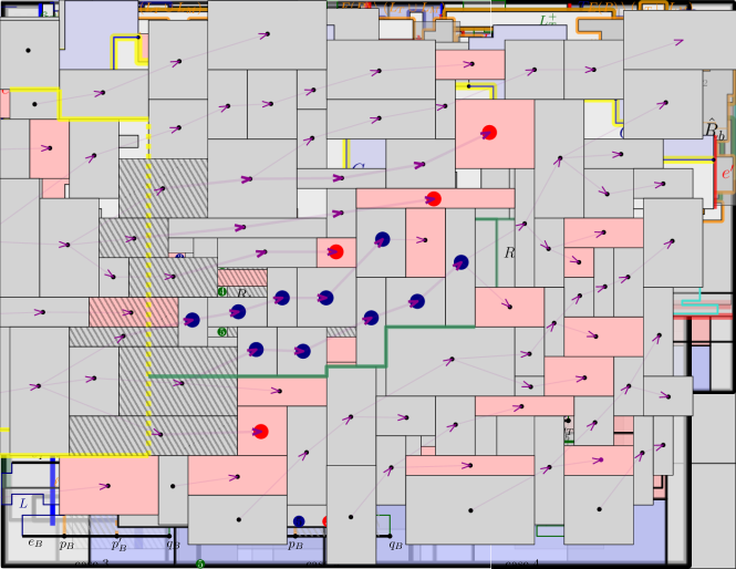
Figure 10: Our cut $C$ (yellow) may partition a simple axis-parallel polygon $P$ into two connected components (blue and gray) that are not simple polygons. In this case, we identify one subpath $C^{\prime}\subset C$ whose interior lies inside $P$ (and thus cuts $P$ into two simple polygons), such that cutting along $C^{\prime}$ does not increase the complexity. For instance here, $C^{\prime}$ may be any of $\{C_{3},C_{4},C_{6},C_{7},C_{8}\}$. On the other hand, cutting $P$ along $C_{1},C_{2}$ of $C_{5}$ would create one simple connected component with strictly more edges than $P$. Indeed, each such subpath $C_{i}$ ($i\in\{1,2,5\}$) connects two edges $e_{i},e^{\prime}_{i}$ of the boundary, that are at distance $d(e_{i},e^{\prime}_{i})\leq c_{i}$, where $c_{i}$ is the number of line segments of $C$ that $C_{i}$ contains. For instance, $2=d(e_{2},e^{\prime}_{2})\leq c_{2}=3$. We show that there exists always a subpath $C_{i}\subset C$ such that $d(e_{i},e^{\prime}_{i})>c_{i}$.

∎

A.3 Charging scheme and analysis.

In this section we show that $|\mathcal{R}^{\prime}|\geq|\mathrm{OPT}|/3$. We use a more sophisticated charging scheme than the one we previously described in Section 3.1. We still follow the same idea of charging non-horizontally nested rectangles that get intersected during the recursive partitioning to corners of rectangles that are not yet intersected. Here either we charge additional corners (that are not necessarily seen by the rectangle that is intersected), or we charge horizontally nested rectangles, and count them as “saved”. This will allow us to charge non-horizontally nested rectangle with a fractional charge of at most $\frac{1}{2}$.

The charging scheme.

Consider an internal node $v$ of the tree and let $\ell_{v}$ be the corresponding line segment $\ell$ defined above for partitioning $P_{v}$ as in Lemma 20. Assume that there is a rectangle $R\subset P_{v}$ that is intersected by $\ell_{v}$ and that is not horizontally nested. By Lemma 20 we know that $R$ is not $7$-protected in $P_{v}$ and, in particular, it is not protected (by a line fence) in $P_{v}$. Thus, Lemma 14 implies that $R$ sees at least one corner of some rectangle in $\mathrm{OPT}^{\prime}(P_{v})$ on each side. For each such rectangle $R$, we introduce $4$ tokens that correspond to a fractional charge of $\frac{1}{4}$ each (we will later refer to these tokens as belonging to $R$). We distribute two tokens on the right and two on the left. Let us describe the token distribution on the right and the token distribution to the left will be symmetric. See Figure 11.

Figure 11: Token distribution strategy for the charging scheme.

Since $R$ is not horizontally nested, it sees at least one corner on its right.

1. If $R$ sees more than one corner, put one token on two of those corners each (choose any two such corners arbitrarily if needed).

2. If $R$ sees only one corner $c$ of a rectangle, say $\hat{R}_{0}\in\mathrm{OPT}^{\prime}$ on its right, then we give one token to $c$. To identify the second corner that will receive the second token from $R$, we first observe the following.

   Claim 23.

   If $c$ is the top-left corner (resp. bottom-left corner) of $\hat{R}_{0}$, then the $y$-coordinates of the top edges (resp. the bottom edges) of $R$ and $\hat{R}_{0}$ are equal and the $x$-coordinates of the right edge of $R$ and left edge of $\hat{R}_{0}$ are equal.

   Proof.

   Let $y_{b}$ and $y_{t}$ denote the $y$-coordinates of the bottom and top edge of $R$, respectively, and let $y^{\prime}_{b}$ and $y^{\prime}_{t}$ denote the $y$-coordinates of the bottom and top edge of $\hat{R}_{0}$, respectively. Additionally, let $x_{r}$ denote the $x$-coordinate of the right edge of $R$ and let $x^{\prime}_{l}$ denote the $x$-coordinate of the left edge of $\hat{R}_{0}$. Observe that in the proof of Lemma 14, the only cases when $R$ sees only one corner to its right are case $1$ when $y_{t}=y^{\prime}_{t}$ and $y^{\prime}_{b}<y_{b}$, and case $2a$ when $y_{t}<y^{\prime}_{t}$ and $y_{b}=y^{\prime}_{b}$. In both these cases we have that $x_{r}=x^{\prime}_{l}$, which completes the proof of the claim. ∎

   We assume without loss of generality that the unique corner $c$ that $R$ sees on its right is the top-left corner of $\hat{R}_{0}$, as the other case can be handled symmetrically. Let $h$ be the rightwards horizontal ray from the top-right vertex $p$ of $R$ and let $\hat{R}_{b}\in\mathrm{OPT}^{\prime}(P_{v})$ be the first rectangle such that $h$ intersects the interior of the left edge of $\hat{R}_{b}$. Notice that such a rectangle must exist, as otherwise the top edge of $R$ would be contained in a 1-fence emerging from a right vertical edge of $P$. This would imply that $R$ is $3$-protected and in particular, it would be $7$-protected, contradicting property (4) of Lemma 20. Let $p^{\prime}$ be the intersection of $h$ with the left edge of $\hat{R}_{b}$. Let $H^{r}_{R}$ be the set of all rectangles in $\mathrm{OPT}^{\prime}(P_{v})$ that have their top edge contained in the horizontal line segment $pp^{\prime}$.

   1. Suppose there exists in $H^{r}_{R}$ a rectangle $\hat{R}_{a}$ that is horizontally nested. Notice that then, the right edge of $\hat{R}_{a}$ has to be contained in the left edge of $\hat{R}_{b}$. In this case, give the second token to the top-left corner of $\hat{R}_{a}$. In particular, in the case when $\hat{R}_{a}=\hat{R}_{0}$, the top-left corner of $\hat{R}_{a}$ has received two tokens from $R$.

   2. If none of the rectangles in $H^{r}_{R}$ are horizontally nested, then give the second token to the bottom-left corner of $\hat{R}_{b}$. (In the case when the bottom edges of $R$ and $\hat{R}_{0}$ have the same $y$-coordinate, we charge the top-left corner of $\hat{R}_{b}$).

We say that the corners of rectangles $\hat{R}_{0},\hat{R}_{a}$ or $\hat{R}_{b}$ in $\mathrm{OPT}^{\prime}$ that received a token from $R$ were charged by $R$. We perform this token distribution for each non-horizontally nested rectangle $R\in OPT^{\prime}$ that is intersected during the recursive partitioning. See Figure 12 for an example of this token distribution.

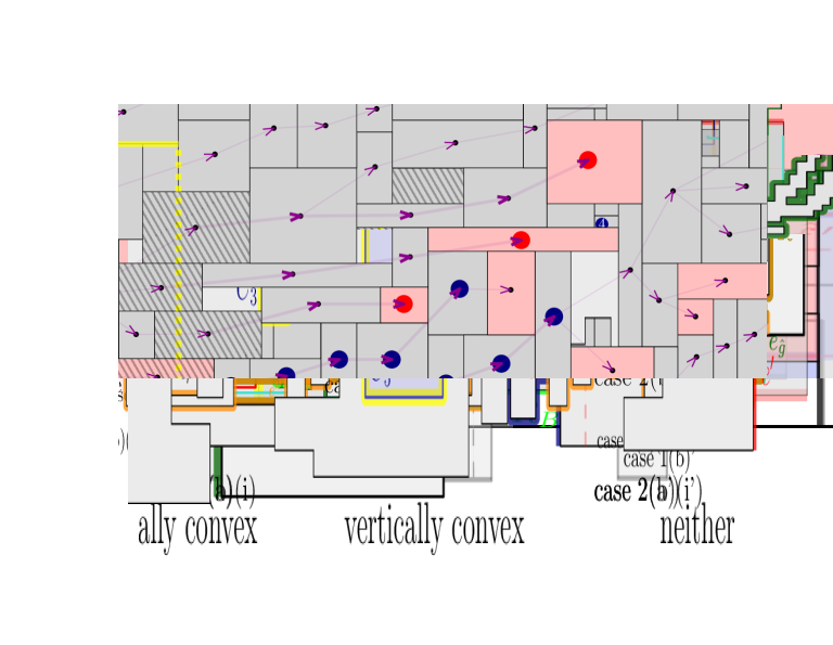
Figure 12: An example of the charging process for rectangles intersected (tilling pattern) by the vertical line segment (dashed yellow line) of a cut (yellow) of a polygon $P$ during the partitioning process. Rectangles in $\mathrm{OPT}^{\prime}(P)$ that are horizontally nested are displayed in red. For each rectangle $R_{i}$ ($1\leq i\leq 5$) that is intersected by $\ell$ and not nested horizontally, we introduce 4 tokens (marked by the number $i$); and we distribute two tokens to corners of rectangles of $\mathrm{OPT}^{\prime}(P)$ on the right, and two on the left. In further iterations of the partitioning process, rectangles that has been charged will be $3$-protected (Lemma 24) and thus will never be intersected. Each corner of a rectangle is charged with at most one token if it is not horizontally nested, and with at most two tokens if it is horizontally nested (Lemma 26). Additionally, if the left corner of a rectangle is charged (for example the bottom-left corner of $\hat{R}$), then all the rectangles on the right of $\hat{R}$ that may potentially charged right corners of $\hat{R}$ (such as $R^{\prime}$), will be protected by $7$-fences (green line segments) emerging from $\ell$, and thus right corners of $\hat{R}$ will not be charged later (Lemma 27).

Analysis of the charging scheme.

We now analyze our charging scheme. We show that following the charging scheme mentioned above, we can guarantee that the number of tokens on a non-horizontally nested rectangle and a horizontally nested rectangle is at most two and four respectively. We show this by first proving that there can be at most one token on a corner of a non-horizontal rectangle and at most two tokens on a corner of a horizontally nested rectangle. Then we prove that only one of the two corners of any horizontal edge of a rectangle can be charged.

To prove these results, we first need to establish the following technical properties.

Lemma 24.

Let $R\in\mathrm{OPT}^{\prime}(P_{v})$ be a non-horizontally nested rectangle intersected during the partitioning of $P_{v}$ for some node $v\in T$, and let $c$ be the left corner of a rectangle $\hat{R}\in\mathrm{OPT}^{\prime}(P_{v})$ charged by $R$. Then we have that:

1. $c$ is seen by $R$ or by the rightmost rectangle on the left of $\hat{R}$ in $H_{R}^{r}$;

2. if $v^{\prime}\in T$ denotes the child of $v$ such that $\hat{R}\subseteq P_{v^{\prime}}\subset P_{v}$, then $\hat{R}$ and all the rectangles in $H^{r}_{R}$ are protected by $3$-fences emerging from a left vertical edge of $P_{v^{\prime}}$.

Proof.

The proof of $(1)$ follows directly if $c$ is seen by $R$ or $\hat{R}\in H^{r}_{R}$ because the right most rectangle to the left of $\hat{R}$ in $H^{r}_{R}$ will belong to $\{R\}\cup H^{r}_{R}$ and it is easy to see that this rectangle will see the corner $c$ of $\hat{R}$ from the proof of Lemma 14. If both conditions do not happen, then corner $c$ is charged via case $2(b)$ of the charging scheme. Let us assume without loss of generality that $c$ is the bottom left corner of $\hat{R}$. The rightward ray from the top right vertex $p$ of $R$ hits the interior of the left edge of $\hat{R}$ at $p^{\prime}$ and the line segment $h$ joining $p$ and $p^{\prime}$ contains the top edges of all the rectangles in $H^{r}_{R}$ by the way we find $\hat{R}$ and $c$ in the charging scheme. The fact that we charged $c$ implies that the rightmost rectangle $\hat{R}_{a}$ in $H^{r}_{R}$ is non-horizontally nested. Since the horizontal line segment $h^{\prime}$ joining the top right vertex of $\hat{R}_{a}$ and $p^{\prime}$ on the left edge of $\hat{R}$ does not intersect any rectangle in $\mathrm{OPT}^{\prime}(P_{v})$ and also does not contain the top edges of any rectangle in $\mathrm{OPT}^{\prime}(P_{v})$, we can say that $\hat{R}_{a}$ has to see the corner $c$ of $\hat{R}$ following a similar argument as in the proof of Lemma 14.

The proof of $(2)$ will follow from the above proof of $(1)$ because, if $c$ is seen by $R$ or $\hat{R}\in H^{r}_{R}$, then after partitioning $P_{v}$, the horizontal line segment connecting $c$ and the left boundary of $P_{v^{\prime}}$ does not intersect any rectangle in $\mathrm{OPT}^{\prime}(P_{v^{\prime}})$. This means that $c$ is contained in a $1$-fence and hence $\hat{R}$ is $3$-protected. If $c$ is seen by the rightmost rectangle $\hat{R}_{a}$ in $H^{r}_{R}$, then we can say that $c$ is in a $3$-fence that basically connects $p,p^{\prime}$ and $c$ in that order. Since $p^{\prime}$ is in the interior of the left edge of $\hat{R}$, we can say that the top edge is also contained in a $3$-fence emerging from the same point as the $3$-fence that contained $c$, proving that $\hat{R}$ is $3$-protected. Rectangles in $H^{r}_{R}$ are protected by $3$-fences because their top edges (assuming $c$ is a top left corner) are contained in the $1$-fence emerging from the point of intersection of the top edge of $R$ with the part of the vertical cut $\ell_{v}$ partitioning $P_{v}$. ∎

The last property of the claim ensures that a rectangle that is charged will be $3$-protected after being charged for the first time, and in particular using Lemma 21(iii) we directly obtain the following property of our charging scheme.

Lemma 25.

If a rectangle $\hat{R}\in\mathrm{OPT}^{\prime}$ is charged, then $\hat{R}\in\mathcal{R}^{\prime}$.

We now bound the number of tokens charged to a corner of a rectangle $\hat{R}\in\mathcal{R}^{\prime}$. This bound depends on whether $\hat{R}$ is horizontally nested or not.

Lemma 26.

Let $\hat{R}\in\mathcal{R}^{\prime}$ be a not horizontally nested (resp. horizontally nested) rectangle. Then, each of its corners is charged with at most one token (resp. at most two tokens).

Proof.

We first distinguish two types of tokens. If the corner $c$ of a rectangle $\hat{R}\in\mathcal{R}^{\prime}$, charged by a rectangle $R\in\mathrm{OPT}^{\prime}$, is seen by $R$, then we say that the corresponding token is a direct token, and that $c$ was directly charged by $R$. Otherwise, we say that it is an indirect token, and that $c$ was indirectly charged by $R$. For instance, in Figure 11, the tokens received by $\hat{R}_{b}$ in case 2(b) and by $\hat{R}_{a}$ in case 2(a) top, are indirect tokens. In Figure 12, direct tokens are shown in green, and indirect tokens are shown in red and blue.

Since a corner of a rectangle in $\mathrm{OPT}^{\prime}$ is seen by at most one rectangle in $\mathrm{OPT}^{\prime}$, a corner cannot be directly charged by two different rectangles. In particular, a rectangle $R$ charges a corner $c$ of a rectangle $\hat{R}$ with one token if either this corner is not the unique corner seen by $R$ on the same side as corner $c$ (see case 1 in Figure 11) or $\hat{R}$ is non-horizontally nested, and with two tokens if $\hat{R}$ is horizontally nested and $c$ is the unique corner seen by $R$ to that side (this happens in the case 2(a), when $\hat{R}_{a}=\hat{R}_{0}$). Moreover, observe that a corner cannot be simultaneously charged directly and indirectly by the same rectangle. We now show that if a corner $c$ of a rectangle $\hat{R}\in\mathcal{R}^{\prime}$ is directly charged by a rectangle $R\in\mathrm{OPT}^{\prime}$, it cannot be also indirectly charged by another rectangle $R^{\prime}\in\mathrm{OPT}^{\prime}$.

For a contradiction, assume that $c$ was directly charged by a rectangle $R$ intersected during the partitioning of $P_{v}$ for some node $v\in T$ and that $c$ was indirectly charged by a rectangle $R^{\prime}\neq R$ that was intersected during the partitioning of $P_{v^{\prime}}$ for some node $v^{\prime}\in T$. We have either $P_{v}=P_{v^{\prime}}$, $P_{v}\subset P_{v^{\prime}}$ or $P_{v^{\prime}}\subset P_{v}$. Notice that from the first property of Lemma 24, it holds that $R\in H^{r}_{R^{\prime}}$.

• If $P_{v}=P_{v^{\prime}}$, then $R$ and $R^{\prime}$ were intersected by the same vertical line. This is a contradiction with the facts that $R$ is in $H^{r}_{R^{\prime}}$ and that all the rectangles in $H^{r}_{R^{\prime}}$ lie strictly on the right of $R^{\prime}$.

• If $P_{v}\subset P_{v^{\prime}}$, then since $R\in H^{r}_{R^{\prime}}$, we know by Lemma 24 that $R$ is $3$-protected in $P_{v}$ which contradicts the fact that it was intersected during the partitioning of $P_{v}$.

• If $P_{v^{\prime}}\subset P_{v}$, then the leftwards horizontal ray from $c$ must intersect the boundary of $P_{v^{\prime}}$ before intersecting any rectangles in $P_{v^{\prime}}$, which contradicts the fact that $R^{\prime}\in\mathrm{OPT}^{\prime}(P_{v^{\prime}})$.

Therefore, a corner of a rectangle in $\mathcal{R}^{\prime}$ cannot be at the same time directly and indirectly charged.

We now claim that a corner of a rectangle $\hat{R}\in\mathcal{R}^{\prime}$ is charged with at most two indirect tokens, and that in this case, $\hat{R}$ must be horizontally nested. This will conclude the proof of the Lemma.

To prove this fact, we first distinguish two types of indirect tokens: the token of type (a) charged to the horizontally nested rectangle $\hat{R}_{a}$ in case 2(a) of the charging process; and the token of type (b), charged to $\hat{R}_{b}$ in case 2(b). In Figure 12, indirect tokens of type (a) and (b) are respectively shown in red and blue.

We show that a corner $c$ of a rectangle $\hat{R}\in\mathcal{R}^{\prime}$ cannot be charged with two indirect tokens of the same type. This implies that if a corner is charged with two indirect tokens, one of these indirect tokens is of type (a), which implies that $\hat{R}$ must be horizontally nested.

1. Suppose for a contradiction that a left corner $c$ of rectangle $\hat{R}$ has been charged with two tokens of type (a) by two distinct rectangles $R$ (intersected during the partitioning of $P_{v}$ for some $v\in T$) and $R^{\prime}$ (intersected during the partitioning of $P_{v^{\prime}}$ for some $v^{\prime}\in T$). We assume without loss of generality that $c$ is the top-left corner, and that $P_{v^{\prime}}\subseteq P_{v}$. Since $\hat{R}\in H_{R}^{r}$ and $\hat{R}\in H_{R^{\prime}}^{r}$, there is minimal horizontal line segment connecting the top edges of $R,R^{\prime}$ and $\hat{R}$ in $P_{v}$ that does not intersect any rectangle in $\mathrm{OPT}^{\prime}(P_{v})$. We obtain a contradiction similarly as before. If $P_{v^{\prime}}=P_{v}$ then we obtain a contradiction with the fact that $R$ and $R^{\prime}$ must be intersected by the same vertical line segment. Otherwise $R^{\prime}$ was not intersected during the partitioning of $P_{v}$. In this case, if $R^{\prime}$ is on the left of $R$, then the leftwards horizontal ray from $c$ must cross the boundary before reaching the top edge of $R^{\prime}$; if not, then by Lemma 24 $R^{\prime}$ must be $3$-protected in $P_{v^{\prime}}$.

2. Suppose a left corner $c$ of a rectangle $\hat{R}$ was charged with two indirect tokens of type (b) by two distinct rectangles $R$ and $R^{\prime}$. We assume here without loss of generality that $c$ is a bottom-left corner. By Lemma 24, we know that $c$ is seen by a rectangle $\hat{R}_{a}\in H^{r}_{R}\cap H^{r}_{R^{\prime}}$. Therefore, $R$ and $R^{\prime}$ are on the left of $\hat{R}_{a}$ and there is an horizontal line segment that contains the top edges of $R,R^{\prime}$ and $\hat{R}_{a}$. Thus, we can argue as in case (a) to obtain a contradiction.

This finishes the proof. ∎

We now show that if a left corner of a rectangle $\hat{R}\in\mathcal{R}^{\prime}$ is charged, then no right corner of this rectangle is charged, and vice-versa. Intuitively, by Lemma 24, we know that if a left corner of $\hat{R}$ has been charged, the top edge $\hat{R}$ will be contained in a 3-fence emerging from the left; by extending this 3-fence to 7-fences, we will protect all rectangles in $\mathrm{OPT}^{\prime}$ that may potentially charge right corners of $\hat{R}$.

Lemma 27.

At most two corners per rectangle in $\mathcal{R}^{\prime}$ are charged.

Proof.

Suppose that the left corner $c$ of a rectangle $\hat{R}$ was charged by a rectangle $R\in\mathrm{OPT}^{\prime}$ intersected during the partitioning of $P_{v}$ for some $v\in T$. First, since we charge left corners on the right and right corners on the left, it is clear that the right corners of $\hat{R}$ cannot be charged by any rectangle intersected during the partitioning of the same polygon $P_{v}$.

Assume for a contradiction that a right corner of $\hat{R}$ was charged by a rectangle $R^{\prime}$ during the partitioning of $P_{v^{\prime}}$ for some node $v^{\prime}\neq v$ such that $\hat{R}\subset P_{v^{\prime}}\subset P_{v}$. By Lemma 24, we know that the top edge of $\hat{R}$ is contained in a $3$-fence $f$ emerging from a left vertical edge of $P_{v^{\prime}}$. Moreover, since $\hat{R}$ was charged by $R^{\prime}$, there exists a point $p^{\prime}$ contained in the right edge of $\hat{R}$ such that there exists an horizontal line segment $h$ that contains $p^{\prime}$ and the top or the bottom edge of $R^{\prime}$, such that $h$ intersects no rectangles in $\mathrm{OPT}^{\prime}$. We now construct a $5$-fence $f^{\prime}$ anchored on a left vertical edge of $P_{v^{\prime}}$ as the union of $f$, the fraction of the right edge of $\hat{R}$ between its top-right corner and $p^{\prime}$, and the horizontal line segment $h$. See Figure 12. Therefore, the top or the bottom edge of $R^{\prime}$ is contained in a $5$-fence, which implies that it is $7$-protected in $P_{v^{\prime}}$, and thus contradicts the assumptions that it was intersected during the partitioning of $P_{v^{\prime}}$. This shows that a rectangle can be charged only on one side. ∎

Combining these three lemmas, we can lower bound the size of $\mathcal{R}^{\prime}$.

Lemma 28.

It holds that $|\mathcal{R}^{\prime}|\geq|\mathrm{OPT}^{\prime}|/3$.

Proof.

Let us define $\mathcal{I}:=\mathrm{OPT}^{\prime}\setminus\mathcal{R}^{\prime}$, the set of rectangles that were intersected during the recursive partitioning process. Let $\mathrm{OPT}^{\prime}_{h}\subset\mathrm{OPT}^{\prime}$ denote the set of rectangles in $\mathrm{OPT}^{\prime}$ that are horizontally nested. By our initial assumption, we have

$$|\mathrm{OPT}^{\prime}_{h}|\leq\frac{1}{2}|\mathrm{OPT}^{\prime}|$$ (1)

By Lemma 25, we know that all the rectangles in $\mathrm{OPT}^{\prime}$ that are charged are in $\mathcal{R}^{\prime}$. Combining lemmas 26 and 27, we know that each rectangle in $\mathcal{R}^{\prime}\cap\mathrm{OPT}^{\prime}_{h}$ is charged with at most $4$ tokens, i.e., for a total fractional charge of $1$, and each rectangle in $\mathcal{R}^{\prime}\setminus\mathrm{OPT}^{\prime}_{h}$ is charged with at most $2$ tokens, i.e., for a total fractional charge of $1/2$. Thus, we deduce that:

$$|\mathcal{I}\setminus\mathrm{OPT}^{\prime}_{h}|\leq|\mathcal{R}^{\prime}\cap\mathrm{OPT}^{\prime}_{h}|+\frac{1}{2}|\mathcal{R}^{\prime}\setminus\mathrm{OPT}^{\prime}_{h}|$$ (2)

Now we have,

$$\frac{3}{2}|\mathcal{I}| =\frac{3}{2}|\mathcal{I}\setminus\mathrm{OPT}^{\prime}_{h}|+\frac{3}{2}|\mathcal{I}\cap\mathrm{OPT}^{\prime}_{h}|$$

$$\leq|\mathcal{R}^{\prime}\cap\mathrm{OPT}^{\prime}_{h}|+\frac{1}{2}|\mathcal{R}^{\prime}\setminus\mathrm{OPT}^{\prime}_{h}|+\frac{1}{2}|\mathcal{I}\setminus\mathrm{OPT}^{\prime}_{h}|+\frac{3}{2}|\mathcal{I}\cap\mathrm{OPT}^{\prime}_{h}|$$

$$=|\mathcal{R}^{\prime}\cap\mathrm{OPT}^{\prime}_{h}|+\frac{1}{2}\big{(}|\mathrm{OPT}^{\prime}|-|\mathrm{OPT}^{\prime}_{h}|-|\mathcal{I}\setminus\mathrm{OPT}^{\prime}_{h}|\big{)}+\frac{1}{2}|\mathcal{I}\setminus\mathrm{OPT}^{\prime}_{h}|+\frac{3}{2}|\mathcal{I}\cap\mathrm{OPT}^{\prime}_{h}|$$

$$=\frac{1}{2}|\mathrm{OPT}^{\prime}|+\frac{1}{2}|\mathcal{R}^{\prime}\cap\mathrm{OPT}^{\prime}_{h}|+|\mathcal{I}\cap\mathrm{OPT}^{\prime}_{h}|$$

$$\leq\frac{1}{2}|\mathrm{OPT}^{\prime}|+|\mathrm{OPT}^{\prime}_{h}|$$

$$\leq\frac{1}{2}|\mathrm{OPT}^{\prime}|+\frac{1}{2}|\mathrm{OPT}^{\prime}|=|\mathrm{OPT}^{\prime}|,$$

where the first and the last inequalities follow from equations (2) and (1), respectively. Thus, at most two thirds of the rectangles in $\mathrm{OPT}^{\prime}$ are intersected during the recursive partitioning process, and in particular $|\mathcal{R}^{\prime}|\geq\frac{1}{3}|\mathrm{OPT}^{\prime}|=\frac{1}{3}|\mathrm{OPT}|$. ∎

This concludes the proof of Theorem 1.

Appendix B An improved $(2+\varepsilon)$ approximation

In this section, we build on the ideas from Section A. We show that by using the same dynamic program and only making slight modifications to the definition of nesting and charging scheme, we can push the approximation factor arbitrarily close to $2$ by using a larger parameter $k$ of the dynamic program. Let us assume that $\frac{1}{\varepsilon}\in\mathbb{N}$ whenever we refer to $\varepsilon$ below.

Definition 29.

A rectangle $R\in\mathrm{OPT}^{\prime}$ is said to be horizontally nice (resp. vertically nice) if $R$ sees the bottom left (resp. top right) corner of some rectangle in $\mathrm{OPT}^{\prime}$ to its right (resp. bottom) or its bottom edge (resp. right edge) is contained in the boundary of $S$.

The below Observation extends Lemma 14 to a more general result without any assumptions about the rectangle whether it is protected or non-horizontally nested.

Observation 30.

For any rectangle $R\in\mathrm{OPT}^{\prime}$, if the horizontal line segment $h$ that connects its top-right corner to a right vertical edge $e^{\prime}$ of $S$

1. Intersects a rectangle in $\mathrm{OPT}^{\prime}$ or contains the top edge of a rectangle in $\mathrm{OPT}^{\prime}$, then if $R^{\prime}\in\mathrm{OPT}^{\prime}$ be the rectangle intersected by $h$, or that has its top side intersected by $h$, that is the closest to $R$. Then either $R$ sees the bottom left corner of $R^{\prime}$ or $y_{t}\leq y_{t}^{\prime},y_{b}^{\prime}<y_{b},x_{r}=x_{l}^{\prime}$, where $y_{t},y_{t}^{\prime},y_{b},y_{b}^{\prime}$ are the $y$-coordinates of the top edges of $R,R^{\prime}$ and bottom edges of $R,R^{\prime}$, respectively, and $x_{r},x_{l}^{\prime}$ are the $x$-coordinates of the right and left edges of $R$ and $R^{\prime}$, respectively.

2. Does not intersect any rectangle nor contains the top edge of any rectangle in $\mathrm{OPT}^{\prime}$, then the right edge of $R$ is contained in the right edge of $S$

In the next proposition, we show that any rectangle in the optimal solution is either horizontally nice or vertically nice.

Proposition 31.

A rectangle $R\in\mathrm{OPT}^{\prime}$ has to be either horizontally nice or vertically nice.

Proof.

For contradiction, let us assume that there exists a rectangle $R\in\mathrm{OPT}^{\prime}$ such that it is neither horizontally nice nor vertically nice. Consider a horizontal line segment $h$ that connects the top-right corner of $R$ to the right vertical edge of $S$. If $h$ intersects some rectangle in $\mathrm{OPT}^{\prime}$ or contains the top edge of some rectangle in $\mathrm{OPT}^{\prime}$, then let $R^{\prime}\in\mathrm{OPT}^{\prime}$ denote the rectangle intersected by $h$, or that has its top side contained in $h$, that is closest to $R$. From Observation 30, we know that either $R$ sees the bottom left corner of $R^{\prime}$ or $y_{t}\leq y_{t}^{\prime},y_{b}^{\prime}<y_{b},x_{r}=x_{l}^{\prime}$, where $y_{t},y_{t}^{\prime},y_{b},y_{b}^{\prime}$ are the $y$-coordinates of the top edges of $R,R^{\prime}$ and bottom edges of $R,R^{\prime}$, respectively, and $x_{r},x_{l}^{\prime}$ are the $x$-coordinates of the right and left edges of $R$ and $R^{\prime}$, respectively. and if $h$ does not intersect any rectangle and does not contain the top edge of any other rectangle in $\mathrm{OPT}^{\prime}$, then again by Observation 30, we know that the right edge of $R$ is contained in the right edge of $S$ contradicting our assumption on $R$. So we have deduced that if a rectangle is not horizontally nice, then there exists a rectangle $R^{\prime}$ (possibly $S$) such that the bottom right vertex of $R$ is strictly contained in the interior of a vertical edge of $R^{\prime}$. Using symmetry, we can also prove that if a rectangle is not vertically nice, then there exists a rectangle $R^{\prime\prime}$(possibly $S$) such that the bottom right vertex of $R$ is strictly contained in the interior of a horizontal edge of $R^{\prime\prime}$. Since $R$ is neither horizontally nice nor vertically nice, we should have two rectangles that have a common interior point in $\mathrm{OPT}^{\prime}$ – contradicting our assumption about rectangles in $\mathrm{OPT}^{\prime}$. ∎

Using Proposition 31, we can assume without loss of generality that the number of horizontally nice rectangles is at least $|\mathrm{OPT}|/2$. Now let us restate the partitioning lemma, where we will use $\tau={4}/{\varepsilon}+3$. See 20

We introduce an (unprocessed) child vertex of $v$ corresponding to each connected component of $P\setminus C$ which completes the processing of $P$.

We apply the above procedure recursively to each unprocessed vertex $v$ of the tree until there are no more unprocessed vertices. Let $T$ denote the tree obtained at the end, and let $\mathcal{R}^{\prime}$ denote the set of all rectangles that we assigned to some leaf during the recursion. For any given $\varepsilon\geq 0$, we show that by using $\tau={4}/{\varepsilon}+1$ in the partition lemma above, we can guarantee that $|\mathcal{R}^{\prime}|\geq|\mathrm{OPT}|/(2+\varepsilon)$.

Lemma 32.

The tree $T$ and the set $\mathcal{R}^{\prime}$ satisfy the following properties.

1. For each node $v\in T$, the horizontal edges of $P_{v}$ do not intersect any rectangle in $\mathrm{OPT}^{\prime}$.

2. $T$ is a $120/\varepsilon+108$-recursive partition for $\mathcal{R}^{\prime}$.

3. If a rectangle $R\in\mathrm{OPT}^{\prime}$ is $(4/\varepsilon+3)$-protected in $P_{v}$ for some node $v\in T$, then

   • it is $(4/\varepsilon+3)$-protected in $P_{v^{\prime}}$ for each descendant $v^{\prime}$ of $v$,

   • $R\in\mathcal{R}^{\prime}$.

Proof.

The first and second properties follow from the definition of the fences and Lemma 20(2) and $\tau={4}/{\varepsilon}+3$. The third property follows from the fact that for any $\tau\geq 1$, if $f$ is a $\tau$-fence in $F(P_{v})$ then, $f\cap P_{v^{\prime}}$ is a $\tau$-fence of $F(P_{v^{\prime}})$. ∎

B.1 Charging scheme and analysis.

To describe our charging scheme, we first define a directed graph $H$ whose vertex set is $\mathrm{OPT}^{\prime}$ and where there is a directed edge from a node corresponding to a rectangle $R\in\mathrm{OPT}^{\prime}$ to that of $\hat{R}\in\mathrm{OPT}^{\prime}$ if and only if $R$ sees the bottom-left corner of $\hat{R}$ on its right. Since a corner of a rectangle can be seen by at most one rectangle on its left, the in-degree of each node in $H$ is at most one. Therefore, $H$ is a directed forest. Notice that in that forest, nodes with out-degree zero correspond to rectangles that are not horizontally nice.

Before presenting formally the charging process, we need the following Claim that gives us a bridge between $\tau$-protection and distances in $H$. For the ease of the presentation, we identify a node in $H$ with its corresponding rectangle in $\mathrm{OPT}^{\prime}$.

Claim 33.

Let $R$ and $R^{\prime}$ be two rectangles in $\mathrm{OPT}^{\prime}$ such that there exists an oriented path in $H$ of length $d$ that connects $R$ to $R^{\prime}$. Then, there exists a sequence $f$ of at most $2d+1$ horizontal and vertical line segments such that $f$ intersects no rectangles in $\mathrm{OPT}^{\prime}$ and such that the bottom edges of $R$ and $R^{\prime}$ are respectively contained in the first and the last horizontal segment of $f$.

Proof.

We prove the claim by induction on $d$. First, if $d=0$, then $R=R^{\prime}$ and we set $f$ as the bottom edge of $R$. Then, assume that $R$ and $R^{\prime}$ are at distance $d\geq 1$ in $H$. Let $\hat{R}$ denote the rectangle incident to ${R^{\prime}}$ on the directed path from $R$ to $R^{\prime}$. By induction hypothesis, there exists a set $\hat{f}$ of at most $2(d-1)+1$ horizontal and vertical line segments that intersects no rectangle in $\mathrm{OPT}^{\prime}$ and whose first and last horizontal segment respectively contain the bottom edge of $R$ and the bottom edge of $R^{\prime}$. Since $\hat{R}$ sees the bottom-left corner of $R^{\prime}$, there is a horizontal line segment $h$ that connects the bottom-right corner of $R^{\prime}$ to a point $x$ on the right edge of $\hat{R}$, without intersecting any rectangle in $\mathrm{OPT}^{\prime}$. We define $f$ as the union of $\hat{f}$, the vertical line segment from the bottom-right corner of $\hat{R}$ to $x$, and $h$. One can easily check that $f$ satisfies the expected properties. This terminates the proof of the claim. ∎

We now describe the charging process. Consider the tree $T$ obtained at the end of the recursive partitioning process. For each node $v\in T$ and each rectangle $R$ intersected by $\ell_{v}$ during the partitioning of $P_{v}$, we proceed as follows. Let $\gamma$ be any maximal oriented path in $H$, rooted at $R$, such that all rectangles in $\gamma$ are contained in $P_{v}$.

1. If $\gamma$ has length at least $2/\varepsilon$, then we distribute a (fractional) charge of $\varepsilon/2$ to each of the first $2/\varepsilon$ rectangles.

2. Otherwise, $\gamma$ has length less than $2/\varepsilon$. Let us denote by $R^{\prime}$ the last rectangle on $\gamma$. Then,

   1. either $R^{\prime}$ is a leaf in $H$, i.e., it is not horizontally nice. In that case, we distribute a charge of $1$ to $R^{\prime}$.

   2. Or, $R^{\prime}$ sees the bottom-left corner of a rectangle $R^{\prime\prime}$ that is not contained in $P_{v}$. Using the Claim above, we deduce that the bottom edge of $R$ is contained in a $(4/\varepsilon+1)$-fence emerging from a right vertical edge of $P_{v}$, i.e., $R$ is $(4/\varepsilon+3)$-protected in $P_{v}$. This is a contradiction with Lemma 20$(4)$ and Lemma 32$(iii)$. Thus, this case cannot happen.

See Figure 13 for an illustration of the charging process. We now discuss the correctness of our charging process. First, since each node in $H$ have in-degree at most one, it is clear that a rectangle cannot be charged by two rectangles intersected by the same vertical line segment $\ell_{v}$. Then, using Claim 33, we know that after being charged, each rectangle on $\gamma$ will be $(4/\varepsilon+3)$-protected in $P_{v^{\prime}}$ for any node $v^{\prime}\in T$ such that $P_{v^{\prime}}\subset P_{v}$, and therefore rectangles that are charged will be part of the final solution $\mathcal{R}^{\prime}$ (Lemma 32$(iii)$).

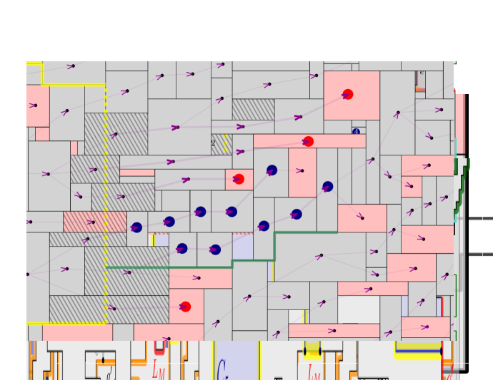
Figure 13: An example of the charging process for the $(2+\varepsilon)$-approximation algorithm with $\varepsilon=\frac{2}{5}$. Rectangles that are not horizontally nice are displayed in red. For each rectangle intersected (tilling pattern) by the vertical line segment (dashed yellow line) of a cut (yellow) of a polygon $P$ during the partitioning process, we will charge some rectangles in $\mathrm{OPT}^{\prime}(P)$ that will be protected by long enough fences (green line segments) in further iterations of recursive partitioning process. To decide which rectangles to charge, we use the directed forest $H$ displayed by purple arcs, and select one directed path (thicker lines) rooted at each rectangle that we need to pay for. When this path is long enough, we distribute a charge (big blue dots) of $\varepsilon/2={1}/{5}$ to each of the $2/\varepsilon=5$ first horizontally nice rectangles. Otherwise, the path ends on a non-horizontally nice rectangle and then we give a full charge of $1$ to this rectangle.

Analysis of the charging scheme.

Now we finally show that $|\mathcal{R}^{\prime}|\geq|\mathrm{OPT}^{\prime}|/(2+\varepsilon)$.

Lemma 34.

It holds that $|\mathcal{R}^{\prime}|\geq|\mathrm{OPT}^{\prime}|/(2+\varepsilon)$.

Proof.

Let $b_{c},b_{\ell},r_{c},r_{\ell}$ be the fraction of blue rectangles that are charged, blue rectangles that are intersected(and hence lost), red rectangles that are charged, and red rectangles that are intersected respectively. Then we have

$$b_{c}+b_{\ell}+r_{c}+r_{\ell} =1$$ (3)

$$r_{c}+r_{\ell} \leq\frac{1}{2}$$ (4)

Here Equation (4) follows from the assumption that at least half of the rectangles are horizontally nice.

Now from the charging scheme, each saved red rectangle will receive a charge of at most $1$ and each saved blue rectangle will receive a charge of at most $\varepsilon/2$. Thus we observe that $b_{\ell}|\mathrm{OPT}^{\prime}|\leq(b_{c}|\mathrm{OPT}^{\prime}|\cdot\varepsilon/2)+r_{c}|\mathrm{OPT}^{\prime}|$. Hence,

$$\frac{2}{\varepsilon}(b_{\ell}-r_{c}) \leq b_{c}$$ (5)

This property of charging is crucial in our analysis.

Multiplying Equation (5) by $\varepsilon$, and Equation (4) by $2$ and then adding them gives

$$2(b_{\ell}+r_{\ell}) \leq\varepsilon b_{c}+1.$$ (6)

Using Equation (3), as $b_{\ell}+r_{\ell}=1-b_{c}+r_{c}$, we obtain

$$1\leq(2+\varepsilon)b_{c}+2(r_{c})\leq(2+\varepsilon)(b_{c}+r_{c}).$$ (7)

This proves that $b_{c}+r_{c}\geq{1}/({2+\varepsilon})$, i.e., $|\mathcal{R}^{\prime}|\geq|\mathrm{OPT}^{\prime}|/(2+\varepsilon)$. ∎

Appendix C Omitted proofs

C.1 Proof of Lemma 2

Polygons associated to the cells of the dynamic program are axis-parallel, have at most $k$ edges, and each vertex has integral coordinates in $[0,\dots,2n-1]\times[0,\dots,2n-1]$. Thus, the number of cells is $O(n^{k})$. For each cell, the algorithm enumerates all possible partitions of the corresponding polygon $P\in\mathcal{P}(k)$ into two or three polygons $P_{1},P_{2},P_{3}$ in $\mathcal{P}(k)$. Such a partition can be characterized by two sequences $\sigma$ and $\sigma^{\prime}$ of line segments whose union corresponds to edges of $P_{i}$ (with $i=1,2,3$) that are contained in the interior of $P$. Since each $P_{i}$ has at most $k$ edges and each such edge is shared by two polygons $P_{i}$, the total number of line segments in $\sigma\cup\sigma^{\prime}$ is at most $3k/2$. Thus, the running time to process each DP cell is $O(n^{3k/2})$. This gives an overall running time of $O(n^{5k/2})$. ∎

C.2 Proof of Lemma 4

Notice that we can assume w.l.o.g. that there is no pair of rectangles $R_{p},R_{q}\in\mathcal{R}$ such that $R_{p}\subseteq R_{q}$ (if that is the case, we can safely replace $R_{q}$ by $R_{p}$ in any feasible solution containing $R_{q}$).

We will prove the statement by induction on the height of the tree. If the tree has height $1$, it means that $|\mathcal{R}^{\prime}|$ is constant and each node aside from the root contains either a unique or no rectangle from $\mathcal{R}^{\prime}$. For each polygon in one of the leaves we can define a feasible partition into a constant number of polygons from $\mathcal{P}$ by circumventing the corresponding rectangle from $\mathcal{R}^{\prime}$ and extending its horizontal boundary until touching the boundary of the polygon. This sequence of polygons represents a feasible partition that our Dynamic Program considers, meaning that the returned solution will have size at least $|\mathcal{R}^{\prime}|$ as the polygons containing the rectangles from $\mathcal{R}^{\prime}$ will be leaves containing a unique rectangle.

Following the inductive proof, we can recurse the argument on each subtree rooted at a child of the root (notice that the subtrees are not $k$-recursive partitions of their corresponding sets of rectangles as the polygons associated to their roots are not $S$; however, that requirement does not play a role in this argumentation so, for the sake of this proof, we can assume that partitions allow to associate arbitrary polygons from $\mathcal{P}$ to the root node). Again the subdivision into polygons induced by the recursive partition for $\mathcal{R}^{\prime}$ is a feasible candidate that our Dynamic Program considers, leading to a returned solution of size at least $|\mathcal{R}^{\prime}|$.∎

C.3 Proof of Lemma 8

Let $\mathcal{T}$ be a $k$-recursive partition for a set $\mathcal{R}^{\prime}\subseteq\mathrm{OPT}^{\prime}$, and consider $\tilde{\mathcal{R}}\subseteq\mathrm{OPT}$ to be the set of original rectangles that were maximally expanded so as to obtain $\mathcal{R}^{\prime}$. In particular $|\mathcal{R}^{\prime}|=|\tilde{\mathcal{R}}|$. Since each rectangle $R\in\tilde{\mathcal{R}}$ is contained in a unique rectangle $R^{\prime}\in{\mathcal{R}^{\prime}}$, we conclude that $\mathcal{T}$ is also a $k$-recursive partition for $\tilde{\mathcal{R}}$. ∎

C.4 Proof of Proposition 9

For a contradiction, assume that a rectangle $R\in\mathrm{OPT}^{\prime}$ is vertically and horizontally nested. W.l.o.g. we can assume that its top edge is contained in the interior of an edge of a rectangle $R^{\prime}\in\mathrm{OPT}^{\prime}$ and its left edge is contained in the interior of an edge of a rectangle $R^{\prime\prime}\in\mathrm{OPT}^{\prime}$. Let $c=(x,y)$ be the coordinates of the top-left corner of $R$. Since $c$ lies in the interior of the bottom edge of $R^{\prime}$ and coordinates of rectangles in $\mathrm{OPT}^{\prime}$ are integral, we deduce that the point $c^{\prime}=(x-1/2,y+1/2)$ must lie in the interior of $R^{\prime}$. An analogous argumentation indicates that $c^{\prime}$ is also contained in the interior of $R^{\prime\prime}$. This is a contradiction with the fact that rectangles in $\mathrm{OPT}^{\prime}$ are disjoint. ∎

C.5 Proof of Lemma 14

Let $R$ be a rectangle in $\mathrm{OPT}^{\prime}(P)$ that is not horizontally nested. We prove that $R$ sees a corner on its right, or is protected. The left case is symmetrical. Consider the horizontal line segment $h$ that connects its top-right corner to a right vertical edge $e^{\prime}$ of $P$. If $h$ does not intersect any rectangle in $\mathrm{OPT}^{\prime}(P)$, then $R$ must be protected by a fence that emerges from a point in $e^{\prime}$, i.e., $R$ is protected in $P$. Otherwise, let $R^{\prime}\in\mathrm{OPT}^{\prime}(P)$ denote the rectangle intersected by $h$, or that has its top side intersected by $h$, that is the closest to $R$. We now use the fact that $R$ is not horizontally nested to prove that $R$ sees a corner of $R^{\prime}$.

Let $y_{b}$ and $y_{t}$ denote the $y$-coordinates of the bottom and top edge of $R$ and let $y^{\prime}_{b}$ and $y^{\prime}_{t}$ denote the $y$-coordinates of the bottom and top edge of $R^{\prime}$. Additionally, let $x_{r}$ denote the $x$-coordinate of the right edge of $R$ and let $x^{\prime}_{l}$ denote the $x$-coordinate of the left edge of $R^{\prime}$. We know that $x_{r}\leq x^{\prime}_{l}$. We now treat all the possible cases.

1. If $y_{t}=y^{\prime}_{t}$ then, by definition of $R^{\prime}$, we obtain directly that $R$ sees the top-left corner of $R^{\prime}$.

   1. Otherwise, we have $y^{\prime}_{b}<y_{t}<y^{\prime}_{t}$.

      1. If $x_{r}=x^{\prime}_{l}$ then necessarily we have that $y_{b}\leq y^{\prime}_{b}$ since we assumed that $R$ was not horizontally nested. In this case, it is clear that $R$ sees the bottom-left corner of $R^{\prime}$.

      2. Otherwise, we have $x_{r}<x^{\prime}_{l}$, and then either $y^{\prime}_{b}<y_{b}$ or $y_{b}\leq y^{\prime}_{b}$.

         1. We show that $y^{\prime}_{b}<y_{b}$ cannot happen. Indeed, assume that $y^{\prime}_{b}<y_{b}$ and consider the rectangular area $W$ with bottom-left corner $(x_{r},y_{b})$ and top-right corner $(x^{\prime}_{l},y_{t})$. In particular, the right edge of $R$ is the left edge of $W$. Since rectangles in $\mathrm{OPT}^{\prime}$ are maximally large in each dimension, $W$ must intersect some rectangle in $\mathrm{OPT}^{\prime}$. By maximality again, there must be a rectangle $R^{\prime\prime}\in\mathrm{OPT}^{\prime}$ that intersects $h$ within $W$, or that has its top side contained in $h$ within $W$. If $R^{\prime\prime}$ is contained in $P$, then we get a contradiction with the definition of $R^{\prime}$. Otherwise, if $R^{\prime\prime}$ is not contained in $P$, then either $R^{\prime\prime}$ is intersected by the boundary of $P$, and by Lemma 12(iii), it must be intersected by a vertical edge of $P$, or $R^{\prime\prime}$ must be contained in the complement of $P$. In both cases, the horizontal rightwards ray from the top-right corner of $R$ must reach the boundary of $P$ before reaching the left edge of $R^{\prime}$. This is a contradiction with the definition of $R^{\prime}$.

         2. If $y_{b}\leq y^{\prime}_{b}$ then we prove that $R$ sees the bottom-left corner of $R^{\prime}$. As in the previous case, consider the rectangular area $W$ with bottom-left corner $(x_{r},y^{\prime}_{b})$ and top-right corner $(x^{\prime}_{l},y_{t})$. If $R$ does not see the bottom-left corner of $R^{\prime}$, then there must be a rectangle in $\mathrm{OPT}^{\prime}$ that intersects $W$. By maximality, this implies that there exists a rectangle $R^{\prime\prime}$ that intersects $h$ or that has its top side contained in $h$. By the same argumentation as before we obtain a contradiction with the definition of $R^{\prime}$. ∎

C.6 Proof of Observation 30

In case $1$, we know from the proof of Lemma 14 that if $R$ is non-horizontally nested, then $R$ sees the bottom left corner of $R^{\prime}$ or $y_{t}=y_{t}^{\prime},y_{b}^{\prime}<y_{b},x_{r}=x_{l}^{\prime}$ (basically the top picture in case $1$ of Figure C.5). When $R$ is horizontally nested, we already have that $y_{t}<y_{t}^{\prime},y_{b}^{\prime}<y_{b},x_{r}=x_{l}^{\prime}$ by the definition of horizontally nestedness. Which completes the proof for this case of the observation. In case $2$, if $R$ is non-horizontally nested, by the exact same arguments as in case $(2.b.i)$ in the proof of Lemma 14(refer to the figure of case $(2.b.i)$ of Figure C.5) , we get a contradiction. Otherwise, the only case for $R$ to be horizontally nested in case $2$ of our observation is if the right edge of $R$ has to be contained in the right edge of $S$. This completes the proof of the observation

C.7 Proof of Lemma 15

Suppose that $R^{\prime}$ receives a charge from a rectangle $R$ during the partitioning of $P_{v}$, for some $v\in T$. In particular, $R$ sees a corner $c$ of $R^{\prime}$. W.l.o.g. we assume that $R^{\prime}$ is on the right of $R$, and $c$ is the top-left corner of $R^{\prime}$ (the case where $c$ is the bottom-left corner is analogous). Consider $v^{\prime}\in T$ to be the child of $v$ such that $P_{v^{\prime}}$ contains $R^{\prime}$. We show that $R^{\prime}$ is protected in $P_{v^{\prime}}$. As discussed before, as a consequence of property (4) of Lemma 12, this will imply that $R^{\prime}\in\mathcal{R}^{\prime}$. The vertical line segment $\ell_{v}$ that intersected $R$ is a vertical edge of $P_{v^{\prime}}$. Since $R$ sees $c$, the horizontal leftwards ray from $c$ does not intersect any rectangle in $\mathrm{OPT}^{\prime}(P_{v^{\prime}})$ and reaches a left vertical edge of $P_{v^{\prime}}$, say on a point $p$. Then, the horizontal edge of $R^{\prime}$ that contains $c$ is contained in the line fence of $F(P_{v^{\prime}})$ emerging from $p$, i.e., $R^{\prime}$ is protected in $P_{v^{\prime}}$. ∎

C.8 Proof of Lemma 16

Let $c$ be a corner of a rectangle $R^{\prime}\in\mathcal{R}^{\prime}$. W.l.o.g. we assume that $c$ lies on the left side of $R^{\prime}$. We also assume that $c$ is the top-left corner of $R^{\prime}$ (the case when $c$ is the bottom-left corner is analogous). For a contradiction, assume that $c$ is charged at least twice. Then, there are two rectangles $R_{1}\in\mathrm{OPT}^{\prime}(P_{v_{1}})$ and $R_{2}\in\mathrm{OPT}^{\prime}(P_{v_{2}})$, for some nodes $v_{1},v_{2}\in T$, such that $c$ receives charges from $R_{1}$ during the partitioning of $P_{v_{1}}$ and also receives charge from $R_{2}$ during the partitioning of $P_{v_{2}}$. In particular, both $R_{1}$ and $R_{2}$ see $c$, and $R^{\prime}\subseteq P_{v_{2}}\cap P_{v_{1}}$. We have $P_{v_{2}}\subseteq P_{v_{1}}$ or $P_{v_{1}}\subseteq P_{v_{2}}$. W.l.o.g. we assume that $P_{v_{2}}\subseteq P_{v_{1}}$. In particular, both $R_{1}$ and $R_{2}$ are contained in $P_{v_{1}}$.

First, if $v_{1}=v_{2}$, then $R_{1}$ and $R_{2}$ are both intersected by the same vertical line segment $\ell_{v_{1}}$ (Lemma 12, property (3)). In particular, the top edge of $R_{2}$ is below the bottom edge of $R_{1}$, or the contrary. Since both $R_{1}$ and $R_{2}$ see $c$, the leftwards horizontal ray $h$ from $c$ intersect the right edges of both $R_{1}$ and $R_{2}$. These two facts together indicate that $h$ intersect the bottom edge of $R_{1}$ and the top edge of $R_{2}$, or the contrary. This brings a contradiction with the third condition of Definition 13.

Otherwise, we have that $v_{2}$ is a descendant of $v_{1}$. We show that the contradiction comes here from the fact that $R_{2}$ must be protected in $P_{v_{2}}$. Since $c$ was charged from $R_{1}$ during the partitioning of $P_{v_{1}}$, the argumentation in the proof of Lemma 15 indicates that $c$ is contained in a line fence $f$ emerging from a right vertical side of $P_{v_{2}}$. In particular, since $R_{2}$ is contained in $P_{v_{2}}$ and sees $c$, it must be that the top edge (or the bottom edge) of $R_{2}$ is contained in $f$; otherwise we would get a contradiction with the assumption that fences in $P_{v_{2}}$ do not penetrate any rectangle in $\mathrm{OPT}^{\prime}(P_{v_{2}})$. This implies that $R_{2}$ must be protected in $P_{v_{2}}$. Thus, by property (4) of Lemma 12, $R_{2}$ cannot be intersected during the partitioning of $P_{v_{2}}$, and $R^{\prime}$ does not receive any charge from $R_{2}$. ∎

C.9 Proof of Lemma 17

We can write $\mathrm{OPT}^{\prime}=\mathrm{OPT}^{\prime}_{h}\cup\mathcal{R}^{\prime}\cup L$, where $\mathrm{OPT}^{\prime}_{h}$ are the rectangles in $\mathrm{OPT}^{\prime}$ that are horizontally nested and $L$ are the rectangles in $\mathrm{OPT}^{\prime}$ not horizontally nested that are intersected by $\ell_{v}$, for some node $v\in T$. Notice that $L\cap\mathcal{R}^{\prime}=\emptyset$. Since a rectangle has $4$ corners, we know from Lemma 16 that each rectangle in $\mathcal{R}^{\prime}$ receives a charge of at most $2$. Then, by Lemma 15, no corners of rectangles in $L$ are charged. Thus, $|L|\leq 2|\mathcal{R}^{\prime}|$. By our initial assumption that at most half of the rectangles in $\mathrm{OPT}^{\prime}$ are horizontally nested, it holds that $|L|+|\mathcal{R}^{\prime}|\geq|\mathrm{OPT}^{\prime}|/2$. Thus, $|\mathcal{R}^{\prime}|\geq|\mathrm{OPT}^{\prime}|/6=|\mathrm{OPT}|/6$. ∎

C.10 Remaining details of proof of Lemma 12

We would like to ensure that $P\setminus C$ has at least two connected components. This is clearly true if $\ell$ or $\overline{pp^{\prime}}$ contain a point in the interior of $P$. Otherwise, $\ell$ is contained in some edge of $P$. If $\ell$ is contained in a left vertical edge $e$ of $P$, then $p=p^{\prime}$ and in particular $p$ is contained in the interior of the left edge of some rectangle $R\in\mathrm{OPT}^{\prime}$. Then, also the top-left corner of $R$ is contained in $e$, and the line segment joining the top-left corner of $R$ with the top-right corner of $R$ is a fence emerging from $e$ that is longer than $f$, which contradicts the choice of $f$. If $\ell$ is contained in a right vertical edge $e^{\prime}$ of $P$, then $\overline{pp^{\prime}}$ must be identical with the top or the bottom edge of $P$ (since otherwise $\overline{pp^{\prime}}$ would contain a point in the interior of $P$). Assume w.l.o.g. that it is the top edge of $P$. In this case, $P\setminus C$ has only one connected component; however, then $\left\lfloor s/3\right\rfloor+1=1$ which implies that $P$ has at most $4s\leq 8$ edges. Therefore, this is an easy case since we can afford to increase the complexity of $P$ substantially by our cut. For example, since in this case $p^{\prime}$ must be the top-right corner of a rectangle $R\in\mathrm{OPT}^{\prime}(P)$, we can define a cut $C^{\prime}$ that consists of the horizontal line segment between $p$ and the top-left corner of $R$, the left edge of $R$, and the bottom edge of $R$. Then, $P\setminus C^{\prime}$ has two (horizontally convex) connected components, each with at most $4s+2\leq 10$ edges each, and $C^{\prime}$ does not intersect any rectangle from $\mathrm{OPT}^{\prime}(P)$.

References

- [1] Fidaa Abed, Parinya Chalermsook, José R. Correa, Andreas Karrenbauer, Pablo Pérez-Lantero, José A. Soto, and Andreas Wiese. On guillotine cutting sequences. In Approximation, Randomization, and Combinatorial Optimization. Algorithms and Techniques (APPROX/RANDOM), volume 40, pages 1–19. Schloss Dagstuhl - Leibniz-Zentrum für Informatik, 2015. doi:10.4230/LIPIcs.APPROX-RANDOM.2015.1.
- [2] Anna Adamaszek, Sariel Har-Peled, and Andreas Wiese. Approximation schemes for independent set and sparse subsets of polygons. J. ACM, 66(4):29:1–29:40, 2019. doi:10.1145/3326122.
- [3] Anna Adamaszek and Andreas Wiese. Approximation schemes for maximum weight independent set of rectangles. In 54th Annual IEEE Symposium on Foundations of Computer Science (FOCS), pages 400–409. IEEE Computer Society, 2013. doi:10.1109/FOCS.2013.50.
- [4] Pankaj K. Agarwal and Jiangwei Pan. Near-linear algorithms for geometric hitting sets and set covers. Discret. Comput. Geom., 63(2):460–482, 2020. doi:10.1007/s00454-019-00099-6.
- [5] Aris Anagnostopoulos, Fabrizio Grandoni, Stefano Leonardi, and Andreas Wiese. A mazing 2+ approximation for unsplittable flow on a path. ACM Trans. Algorithms, 14(4):55:1–55:23, 2018. doi:10.1145/3242769.
- [6] Nikhil Bansal, Alberto Caprara, and Maxim Sviridenko. A new approximation method for set covering problems, with applications to multidimensional bin packing. SIAM J. Comput., 39(4):1256–1278, 2009. doi:10.1137/080736831.
- [7] Nikhil Bansal, Amit Chakrabarti, Amir Epstein, and Baruch Schieber. A quasi-ptas for unsplittable flow on line graphs. In Proceedings of the 38th Annual ACM Symposium on Theory of Computing (STOC), pages 721–729. ACM, 2006. doi:10.1145/1132516.1132617.
- [8] Nikhil Bansal and Arindam Khan. Improved approximation algorithm for two-dimensional bin packing. In Proceedings of the Twenty-Fifth Annual ACM-SIAM Symposium on Discrete Algorithms (SODA), pages 13–25. SIAM, 2014. doi:10.1137/1.9781611973402.2.
- [9] Nikhil Bansal, Andrea Lodi, and Maxim Sviridenko. A tale of two dimensional bin packing. In 46th Annual IEEE Symposium on Foundations of Computer Science (FOCS), pages 657–666. IEEE Computer Society, 2005. doi:10.1109/SFCS.2005.10.
- [10] Amotz Bar-Noy, Reuven Bar-Yehuda, Ari Freund, Joseph Naor, and Baruch Schieber. A unified approach to approximating resource allocation and scheduling. J. ACM, 48(5):1069–1090, 2001. doi:10.1145/502102.502107.
- [11] Reuven Bar-Yehuda, Michael Beder, and Dror Rawitz. A constant factor approximation algorithm for the storage allocation problem. Algorithmica, 77(4):1105–1127, 2017. doi:10.1007/s00453-016-0137-8.
- [12] Paul S. Bonsma, Jens Schulz, and Andreas Wiese. A constant-factor approximation algorithm for unsplittable flow on paths. SIAM J. Comput., 43(2):767–799, 2014. doi:10.1137/120868360.
- [13] Amit Chakrabarti, Chandra Chekuri, Anupam Gupta, and Amit Kumar. Approximation algorithms for the unsplittable flow problem. Algorithmica, 47(1):53–78, 2007. doi:10.1007/s00453-006-1210-5.
- [14] Parinya Chalermsook. Coloring and maximum independent set of rectangles. In 14th International Workshop on Approximation, Randomization, and Combinatorial Optimization (APPROX/RANDOM), volume 6845, pages 123–134. Springer, 2011. doi:10.1007/978-3-642-22935-0\_11.
- [15] Parinya Chalermsook and Julia Chuzhoy. Maximum independent set of rectangles. In Proceedings of the Twentieth Annual ACM-SIAM Symposium on Discrete Algorithms (SODA), pages 892–901. SIAM, 2009. URL: http://dl.acm.org/citation.cfm?id=1496770.1496867.
- [16] Parinya Chalermsook and Bartosz Walczak. Coloring and maximum weight independent set of rectangles. In Proceedings of the 2021 ACM-SIAM Symposium on Discrete Algorithms (SODA), pages 860–868. SIAM, 2021. doi:10.1137/1.9781611976465.54.
- [17] Timothy M. Chan and Elyot Grant. Exact algorithms and apx-hardness results for geometric packing and covering problems. Comput. Geom., 47(2):112–124, 2014. doi:10.1016/j.comgeo.2012.04.001.
- [18] Timothy M. Chan, Elyot Grant, Jochen Könemann, and Malcolm Sharpe. Weighted capacitated, priority, and geometric set cover via improved quasi-uniform sampling. In Proceedings of the Twenty-Third Annual ACM-SIAM Symposium on Discrete Algorithms (SODA), pages 1576–1585. SIAM, 2012. doi:10.1137/1.9781611973099.125.
- [19] Timothy M. Chan and Sariel Har-Peled. Approximation algorithms for maximum independent set of pseudo-disks. Discret. Comput. Geom., 48(2):373–392, 2012. doi:10.1007/s00454-012-9417-5.
- [20] Bernard Chazelle. A theorem on polygon cutting with applications. In 23rd Annual Symposium on Foundations of Computer Science, Chicago, Illinois, USA, 3-5 November 1982, pages 339–349. IEEE Computer Society, 1982. URL: https://doi.org/10.1109/SFCS.1982.58, doi:10.1109/SFCS.1982.58.
- [21] Chandra Chekuri, Sariel Har-Peled, and Kent Quanrud. Fast lp-based approximations for geometric packing and covering problems. In Proceedings of the 2020 ACM-SIAM Symposium on Discrete Algorithms (SODA), pages 1019–1038. SIAM, 2020. doi:10.1137/1.9781611975994.62.
- [22] Henrik I. Christensen, Arindam Khan, Sebastian Pokutta, and Prasad Tetali. Approximation and online algorithms for multidimensional bin packing: A survey. Comput. Sci. Rev., 24:63–79, 2017. doi:10.1016/j.cosrev.2016.12.001.
- [23] Julia Chuzhoy and Alina Ene. On approximating maximum independent set of rectangles. In IEEE 57th Annual Symposium on Foundations of Computer Science (FOCS), pages 820–829. IEEE Computer Society, 2016. doi:10.1109/FOCS.2016.92.
- [24] Mark de Berg, Otfried Cheong, Marc J. van Kreveld, and Mark H. Overmars. Computational geometry: algorithms and applications, 3rd edition. Springer, 2008. URL: https://www.worldcat.org/oclc/227584184.
- [25] Jeffrey S. Doerschler and Herbert Freeman. A rule-based system for dense-map name placement. Commun. ACM, 35(1):68–79, 1992. doi:10.1145/129617.129620.
- [26] Thomas Erlebach, Klaus Jansen, and Eike Seidel. Polynomial-time approximation schemes for geometric intersection graphs. SIAM J. Comput., 34(6):1302–1323, 2005. doi:10.1137/S0097539702402676.
- [27] Jacob Fox and János Pach. Computing the independence number of intersection graphs. In Proceedings of the Twenty-Second Annual ACM-SIAM Symposium on Discrete Algorithms (SODA), pages 1161–1165. SIAM, 2011. doi:10.1137/1.9781611973082.87.
- [28] Takeshi Fukuda, Yasuhiko Morimoto, Shinichi Morishita, and Takeshi Tokuyama. Data mining using two-dimensional optimized accociation rules: Scheme, algorithms, and visualization. pages 13–23, 1996. doi:10.1145/233269.233313.
- [29] Waldo Gálvez, Fabrizio Grandoni, Afrouz Jabal Ameli, Klaus Jansen, Arindam Khan, and Malin Rau. A tight (3/2+) approximation for skewed strip packing. In Approximation, Randomization, and Combinatorial Optimization. Algorithms and Techniques (APPROX/RANDOM), volume 176, pages 44:1–44:18. Schloss Dagstuhl - Leibniz-Zentrum für Informatik, 2020. doi:10.4230/LIPIcs.APPROX/RANDOM.2020.44.
- [30] Waldo Gálvez, Fabrizio Grandoni, Sandy Heydrich, Salvatore Ingala, Arindam Khan, and Andreas Wiese. Approximating geometric knapsack via l-packings. In 58th IEEE Annual Symposium on Foundations of Computer Science (FOCS), pages 260–271. IEEE Computer Society, 2017. doi:10.1109/FOCS.2017.32.
- [31] Waldo Gálvez, Fabrizio Grandoni, Arindam Khan, Diego Ramírez-Romero, and Andreas Wiese. Improved approximation algorithms for 2-dimensional knapsack: Packing into multiple l-shapes, spirals, and more. In 37th International Symposium on Computational Geometry (SoCG), volume 189, pages 39:1–39:17. Schloss Dagstuhl - Leibniz-Zentrum für Informatik, 2021. doi:10.4230/LIPIcs.SoCG.2021.39.
- [32] Fabrizio Grandoni, Stefan Kratsch, and Andreas Wiese. Parameterized approximation schemes for independent set of rectangles and geometric knapsack. In 27th Annual European Symposium on Algorithms (ESA), volume 144, pages 53:1–53:16. Schloss Dagstuhl - Leibniz-Zentrum für Informatik, 2019. doi:10.4230/LIPIcs.ESA.2019.53.
- [33] Fabrizio Grandoni, Tobias Mömke, Andreas Wiese, and Hang Zhou. A (5/3 + )-approximation for unsplittable flow on a path: placing small tasks into boxes. In Proceedings of the 50th Annual ACM SIGACT Symposium on Theory of Computing (STOC), pages 607–619. ACM, 2018. doi:10.1145/3188745.3188894.
- [34] Rolf Harren, Klaus Jansen, Lars Prädel, and Rob van Stee. A -approximation for strip packing. Comput. Geom., 47(2):248–267, 2014. doi:10.1016/j.comgeo.2013.08.008.
- [35] Johan Håstad. Clique is hard to approximate within . Acta Mathematica, 182(1):105–142, 1999. doi:10.1007/BF02392825.
- [36] Jan-Henrik Haunert and Tobias Hermes. Labeling circular focus regions based on a tractable case of maximum weight independent set of rectangles. In Proceedings of the 2nd ACM International Workshop on Interacting with Maps, MapInteract (SIGSPATIAL), pages 15–21. ACM, 2014. doi:10.1145/2677068.2677069.
- [37] Klaus Jansen and Lars Prädel. New approximability results for two-dimensional bin packing. Algorithmica, 74(1):208–269, 2016. doi:10.1007/s00453-014-9943-z.
- [38] Klaus Jansen and Malin Rau. Closing the gap for pseudo-polynomial strip packing. In 27th Annual European Symposium on Algorithms (ESA), volume 144, pages 62:1–62:14. Schloss Dagstuhl - Leibniz-Zentrum für Informatik, 2019. doi:10.4230/LIPIcs.ESA.2019.62.
- [39] Klaus Jansen and Guochuan Zhang. On rectangle packing: maximizing benefits. In J. Ian Munro, editor, Proceedings of the Fifteenth Annual ACM-SIAM Symposium on Discrete Algorithms (SODA), pages 204–213. SIAM, 2004. URL: http://dl.acm.org/citation.cfm?id=982792.982822.
- [40] Arindam Khan, Arnab Maiti, Amatya Sharma, and Andreas Wiese. On guillotine separable packings for the two-dimensional geometric knapsack problem. In 37th International Symposium on Computational Geometry (SoCG), volume 189, pages 48:1–48:17. Schloss Dagstuhl - Leibniz-Zentrum für Informatik, 2021. doi:10.4230/LIPIcs.SoCG.2021.48.
- [41] Arindam Khan and Madhusudhan Reddy Pittu. On guillotine separability of squares and rectangles. In Approximation, Randomization, and Combinatorial Optimization. Algorithms and Techniques (APPROX/RANDOM), volume 176, pages 47:1–47:22. Schloss Dagstuhl - Leibniz-Zentrum für Informatik, 2020. doi:10.4230/LIPIcs.APPROX/RANDOM.2020.47.
- [42] Sanjeev Khanna, S. Muthukrishnan, and Mike Paterson. On approximating rectangle tiling and packing. In Proceedings of the Ninth Annual ACM-SIAM Symposium on Discrete Algorithms (SODA), pages 384–393. ACM/SIAM, 1998. URL: http://dl.acm.org/citation.cfm?id=314613.314768.
- [43] Liane Lewin-Eytan, Joseph Naor, and Ariel Orda. Routing and admission control in networks with advance reservations. In 5th International Workshop on Approximation Algorithms for Combinatorial Optimization (APPROX), volume 2462, pages 215–228. Springer, 2002. doi:10.1007/3-540-45753-4\_19.
- [44] Dániel Marx. Efficient approximation schemes for geometric problems? In 13th Annual European Symposium on Algorithms (ESA), volume 3669, pages 448–459. Springer, 2005. doi:10.1007/11561071\_41.
- [45] Joseph S. B. Mitchell. Approximating maximum independent set for rectangles in the plane. CoRR, abs/2101.00326, 2021. Version 1. URL: https://arxiv.org/abs/2101.00326v1.
- [46] Joseph S. B. Mitchell. Approximating maximum independent set for rectangles in the plane. CoRR, abs/2101.00326, 2021. Version 3. URL: https://arxiv.org/abs/2101.00326v3.
- [47] Tobias Mömke and Andreas Wiese. Breaking the barrier of 2 for the storage allocation problem. In 47th International Colloquium on Automata, Languages, and Programming (ICALP), volume 168, pages 86:1–86:19. Schloss Dagstuhl - Leibniz-Zentrum für Informatik, 2020. doi:10.4230/LIPIcs.ICALP.2020.86.
- [48] Nabil H. Mustafa, Rajiv Raman, and Saurabh Ray. Settling the apx-hardness status for geometric set cover. In 55th IEEE Annual Symposium on Foundations of Computer Science (FOCS), pages 541–550. IEEE Computer Society, 2014. doi:10.1109/FOCS.2014.64.
- [49] Nabil H. Mustafa and Saurabh Ray. Improved results on geometric hitting set problems. Discret. Comput. Geom., 44(4):883–895, 2010. doi:10.1007/s00454-010-9285-9.
- [50] Frank Nielsen. Fast stabbing of boxes in high dimensions. Theor. Comput. Sci., 246(1-2):53–72, 2000. doi:10.1016/S0304-3975(98)00336-3.
- [51] János Pach and Gábor Tardos. Cutting glass. Discret. Comput. Geom., 24(2-3):481–496, 2000. doi:10.1007/s004540010050.