Differentially Private Densest Subgraph

Abstract

Given a graph, the densest subgraph problem asks for a set of vertices such that the average degree among these vertices is maximized. Densest subgraph has numerous applications in learning, e.g., community detection in social networks, link spam detection, correlation mining, bioinformatics, and so on. Although there are efficient algorithms that output either exact or approximate solutions to the densest subgraph problem, existing algorithms may violate the privacy of the individuals in the network, e.g., leaking the existence/non-existence of edges.

In this paper, we study the densest subgraph problem in the framework of the differential privacy, and we derive upper and lower bounds for this problem. We show that there exists a linear-time $\epsilon$-differentially private algorithm that finds a 2-approximation of the densest subgraph with an extra poly-logarithmic additive error. Our algorithm not only reports the approximate density of the densest subgraph, but also reports the vertices that form the dense subgraph.

Our upper bound almost matches the famous $2$-approximation by Charikar both in performance and in approximation ratio, but we additionally achieve differential privacy. In comparison with Charikar’s algorithm, our algorithm has an extra poly-logarithmic additive error. We partly justify the additive error with a new lower bound, showing that for any differentially private algorithm that provides a constant-factor approximation, a sub-logarithmic additive error is inherent.

We also practically study our differentially private algorithm on real-world graphs, and we show that in practice the algorithm finds a solution which is very close to the optimal.

1 Introduction

The densest subgraph problem (DSP) [16] is a fundamental tool to many graph mining applications. Given an undirected graph $G=(V,E)$, the density of an induced subgraph $S\subseteq V$ is defined as $d_{G}(S)=|E(S)|/|S|$, where $E(S)$ is the set of all edges in the subgraph induced by the vertices $S\subseteq V$. In the densest subgraph problem, the goal is to find a subset of vertices $S\subseteq V$ with the highest density $d_{G}(S)$. The densest subgraph problem (DSP) is used as a crucial tool for community detection in social network graphs. This problem also has notable applications in learning including link spam detection [14], correlation mining [31], story identification [1] and bioinformatics [32] – we refer the reader to the tutorial by Gionis and Tsourakakis [15] for more applications of DSP. Due to its importance, the DSP problem has been studied extensively in the literature [16, 7, 24, 33, 34, 4]: it is long known that efficient, polynomial-time algorithms exist for finding the exact solution of DSP [16, 7, 24].

In many applications of DSP, however, the underlying graph is privacy sensitive (e.g., social network graphs). Therefore, one might be concerned that the result output by the DSP algorithm might breach the privacy privacy of the individuals in the network, e.g., disclose the (non)-existence of friendship between pairs of individuals. In this paper, we explore how to perform community detection on sensitive graphs, while protecting individuals’ privacy. To this end, we ask the following question,

We first help the reader recall the notion of differential privacy [8] in a graph context. Let $G$ and $G^{\prime}$ be two graphs that are identical expect the existence/non-existence of a single edge. Informally, the differential privacy requires that the outputs of the (randomized) algorithm on $G$ and $G^{\prime}$ are close in distribution. In this way, the output of the algorithm does not reveal meaningful information about the existence of an edge in the graph. Henceforth, we say that two undirected graphs $G$ and $G^{\prime}$ are neighboring if they differ in only one edge. More formally, differential privacy (DP) is defined as follows [8].

Definition 1.1 ($(\epsilon,\delta)$-Differential Privacy (DP)).

Let $\epsilon>0$ and $\delta\in[0,1]$. We say that a randomized algorithm ${\sf Alg}$ achieves $(\epsilon,\delta)$-differential privacy or $(\epsilon,\delta)$-DP for short, if for any two neighboring graphs $G$ and $G^{\prime}$, for any subset $U$ of the output space,

$$\Pr[{\sf Alg}(G)\in U]\leq e^{\epsilon}\cdot\Pr[{\sf Alg}(G^{\prime})\in U]+\delta$$

Whenever $\delta=0$, we also say that the algorithm satisfies $\epsilon$-DP.

For the densest subgraph problem, we assume that the output contains 1) a dense subset of vertices $S\subseteq V$; and 2) an estimate of the density of $S$. Had we required the algorithm to output only an estimate of $\max_{S\subseteq V}d_{G}(S)$, i.e., an estimated density of the densest subgraph, then it would have been easy to devise a DP algorithm: observe that the quantity $\max_{S\subseteq V}d_{G}(S)$ has small global sensitivity, that is, if we flip the existence of a single edge in $G$, the quantity $\max_{S\subseteq V}d_{G}(S)$ changes by at most $1$. As a result, we can just use the standard Laplacian mechanism [8] to output a DP estimate with good accuracy. However, we stress that most interesting applications would also want to know the dense community $S$ — simply knowing an estimate of its density would not be too useful.

The requirement to also report a dense vertex set $S\subseteq V$ makes it much more challenging to devise a DP algorithm. In our case, none of the off-the-shelf DP mechanisms would directly work to the best of our knowledge. First, observe that the output is high-dimensional, and has high global sensitivity as we explain in Appendix A. Therefore, the standard Laplacian mechanism [8, 36, 11] (also called output perturbation) completely fails. Another naïve approach is randomized response [37, 36, 11] (also called input perturbation), i.e., adding some noise to obfuscate the existence of each edge. Unfortunately, as we argue in Appendix A, the randomized response approach gives poor utility. Finally, the exponential mechanism [26, 36, 11] also fails — not only is it not polynomial-time, the standard analysis gives an error bound as large as $O(n)$ which makes the result meaningless.

1.1 Our Results and Contributions

We present new upper- and lower-bounds for the differentially private, densest subgraph problem. First, we give a linear-time DP approximation algorithm for the densest subgraph problem. The runtime and accuracy of our algorithm are roughly competitive to the state-of-the-art non-private approximation algorithm by Charikar [7]. Specifically, let $n$ denote the number of vertices. Our algorithm is linear-time, and achieves $\epsilon$-DP and $(2,O(\frac{1}{\epsilon}\log^{2.5}n))$-approximation — here we have two approximation parameters: the first parameter $2$ is the multiplicative approximation ratio, and the second parameter $O(\frac{1}{\epsilon}\log^{2.5}n)$ is an additive error. In comparison, Charikar’s famous (non-private) linear-time algorithm achieves $(2,0)$-approximation where the additive error is $0$. We justify the extra additive error with a new lower bound, showing that to achieve any constant-multiplicative approximation, some sub-logarithmic additive error is unavoidable. Our upper- and lower-bound results are stated in the following theorems:

Theorem 1.2 (DP approximation of densest subgraph).

Given a graph $G$, and parameters $\epsilon>0$ and $\sigma\in[0,1]$, there exists a linear-time $\epsilon$-DP algorithm that succeeds with the probability of $1-\sigma$ and outputs $S\subseteq V$ and an estimate $d^{*}$ such that

$$OPT/2-O(\frac{1}{\epsilon}\cdot\log^{2.5}n\cdot\log\frac{1}{\sigma})\leq d_{G}(S)\leq OPT,\ \ \text{ and }\ \ |d^{*}-d_{G}(S)|\leq O(\frac{1}{\epsilon}\cdot\log^{2.5}n\cdot\log\frac{1}{\sigma})$$

where $OPT$ is the true density of the densest subgraph.

Theorem 1.3 (Lower bound on additive error for DP densest subgraph).

Let $\alpha>1$, $\epsilon>0$ be arbitrary constants, $\exp(-n^{0.49})<\sigma<0.000001\cdot\min(1,\epsilon,\exp(-\epsilon))$, and $0\leq\delta\leq\frac{\sigma\epsilon}{\log\frac{1}{4\sigma}}$. Then, there exists a sufficiently small $\beta=\Theta\big{(}\frac{1}{\alpha}\sqrt{\frac{1}{\epsilon}\log\frac{1}{\sigma}}\big{)}$ such that there does not exist an $(\epsilon,\delta)$-DP mechanism that achieves $(\alpha,\beta)$-approximation with $1-\sigma$ probability.

Note that our upper bound achieves $\epsilon$-DP, and our lower bound works even for $(\epsilon,\delta)$-DP. This makes both our upper- and lower-bounds stronger. The proof of Theorem 1.3 is available in Appendix D. Finally, we conclude the paper in Section 5 by demonstrating the performance of our algorithm on real-world datasets. We show that in practice, our algorithm achieves a very accurate solution, even for small choices of the privacy parameter $\epsilon$.

1.2 Technical Highlight

To see the intuition behind our final algorithm, it helps to break it down into several intermediate steps, to see how the various techniques are eventually woven together.

Background on Charikar’s famous algorithm.

Our algorithm is inspired by a work of Charikar [7]. Charikar [7] shows that a simple greedy algorithm can achieve a multiplicative approximation ratio of $2$ for DSP. The greedy algorithm is as follows. Let $G=(V,E)$ be an undirected graph. Initially, let $S:=V$, i.e., $S$ is initalized to the set of all vertices. At each iteration, the algorithm finds a vertex $v_{\min}\in S$ with the minimum degree in the graph induced by the vertices of $S$, and removes $v_{\min}$ from $S$. Consider an algorithm that repeats the aforementioned procedure until the set $S$ becomes empty. From all of the sets $S$ encountered during the execution of the algorithm, the algorithm returns the one with the highest density. Charikar proved that this simple greedy algorithm achieves an approximation ratio of $2$.

Warmup idea: a quadratic-time DP algorithm.

Our first idea is as follows. In Charikar’s algorithm, in each iteration, all residual vertices $v\in S$ examine their degree within the subgraph induced by $S$ — henceforth we call the the degree of $v$ in the subgraph induced by $S$ the residual degree of $v$. Charikar’s algorithm picks the $v$ with the minimum residual degree and removes it from $S$. Our idea is to replace the residual degree with a noisy, DP counterpart. Unfortunately, naïvely adding independent noise to the true residual degree in each of the $n$ iterations would result in an $n$-fold loss in error given a fixed privacy budget $\epsilon$ (and the loss can be reduced to $\sqrt{n}$ if we allowed $(\epsilon,\delta)$-DP rather than $\epsilon$-DP and used the advanced composition theorem [12, 36, 11]).

Our idea is to rely on the elegant DP prefix sum mechanism by Dwork et al. [9] and Chan, Shi, and Song [5, 6]. Specifically, we can think of the problem as follows.

• Initially, every vertex computes its noisy total degree using the standard Laplacian mechanism. Although there are $n$ vertices, we only need to add noise of constant average magnitude by using parallel composition.

• Next, every vertex $u$ still remaining in $S$ maintains a noisy counter to keep track of roughly how many of its direct neighbors have departed (i.e., have been removed from $S$). If we subtract this value from the vertice’s noisy total degree, we get an estimate of its residual degree in the subgraph induced by $S$.

Therefore, the problem boils down to how to have every residual vertex $v$ maintain a noisy counter of how many of its neighbors have departed. Imagine that every time a neighbor of $v$ departs, a value of $1$ is accumulated to $v$’s counter; and every time a non-neighbor of $u$ departs, $0$ is accumulated to $v$’s counter. Using the elegant DP prefix sum mechanism by Dwork et al. [9] and Chan et al. [5, 6], we can report $v$’s noisy counter value at any time step, incurring only $O(\frac{1}{\epsilon}\cdot{{\sf poly}}\log n)$ error with all but negligible probability. The noisy counter values and the vertices’ noisy degrees are then used to determine which vertex is to depart next. Further, although it seems like there are $n$ counters, using parallel composition, we need not incur extra loss in the privacy budget due to the $n$ counters.

By extending Charikar’s proof (which we omit in this short roadmap), we can prove that this warmup algorithm achieves the desired $(2,\frac{1}{\epsilon}\cdot{{\sf poly}}\log n)$-approximation. In particular, the error of the prefix sum mechanism directly contributes to the additive error term. Unfortunately, the warmup algorithm incurs $\Theta(n^{2})$ runtime, since we need to update $O(n)$ noisy counters in each of the $n$ iterations.

Making it quasilinear time.

Our final goal is to get an $O(m+n)$-time algorithm where $m$ denotes the number of edges and $n$ denotes the number of vertices. However, as an important stepping stone, let us first consider how to make it quasilinear time in $m+n$. The key observation is that when the graph is sparse, updates to the vertices’ noisy counters (realized by the prefix sum mechanisms) are also sparse. Most of the $n^{2}$ updates come with an input $0$, and only $m$ of them come with an input of $1$. Our idea is therefore to avoid triggering updates when the input is $0$.

While the intuition seems simple, realizing this idea differentially privately is actually tricky since we need to avoid consuming too much privacy budget. At a very high level, each vertex $v\in S$ keeps track of a noisy outstanding counter ${\sf Cnt}(v)$ of the number of its neighbors that departed recently, but have not been accumulated into the prefix sum mechanism yet. When a vertex $u$ gets removed from $S$, it informs its neighboring vertices to update their noisy outstanding counters. At this moment, each vertex $v$ also checks if its noisy outstanding counter ${\sf Cnt}(v)$ has exceeded some predetermined polylogarithmic noisy threshold — if so, it accumulates the current outstanding counter into its prefix sum mechanism, and resets ${\sf Cnt}(v)$ to $0$.

The key technical challenge here is that we would be invoking with high probability the total of $O(m)$ updates to the vertices’ noisy outstanding counters, but we cannot afford an $O(m)$-fold loss in the privacy budget (or equivalently, an $O(m)$-fold loss in error when the privacy budget is fixed). To resolve this problem, our idea is in spirit reminiscent of the sparse-vector technique [10, 30, 20].We show that we can reduce the privacy analysis of our algorithm to the standard sparse-vector technique. See the subsequent “proof techniques” paragraph regarding the technical challenges in the analysis and proof.

Final touches: making it linear time.

The above algorithm can be implemented in $O(m+n)\log n$ time if we use a Fibonacci heap to store the residual vertices based on their residual degree (i.e., degree in the graph induced by $S$). To make the algorithm linear time, we discretize vertices residual degree into polylogarithmically sized regions, and place each vertice in a corresponding bucket based on its residual degree.

Using an idea inspired by Charikar [7], one can show that if a vertex is removed from the $k$-th bucket in the current iteration, then, in the next iteration, we only need to sequentially look at the $(k-1)$-th, $k$-th, and $(k+1)$-th, … buckets. Moreover, within each bucket, all vertices are treated as having roughly the same degree, and we do not further differentiate them in picking the next vertex to remove from $S$. Using appropriate data structures to store the buckets and the vertices within the buckets, we can eventually obtain a DP-algorithm that completes in $O(m+n)$ runtime. Here, the discretization due to bucketing introduces some additive polylogarithmic error, but asymptotically we still preserve the $(2,O(\frac{1}{\epsilon}\log^{2.5}n))$-approximation as before. We defer the detailed algorithm and analysis to Section 4.

Proof techniques.

Proving our algorithm DP turns out to be rather non-trivial. Specifically, our algorithm is not a simple sequential composition of the various underlying building blocks (e.g., prefix sum mechanism, and outstanding counter threshold queries). Therefore, we cannot simply analyze each building block separately and then use standard composition theorems to get the desired DP guarantees. The problem is that the building blocks are interleaved in an adaptive way: the outcome of one step of the prefix sum mechanism corresponding to some vertex will affect the input to the next step of some outstanding counter query, which will then affect the input to the next step of prefix sum mechanism. Despite the complex and adaptive nature of our algorithm, we show that the privacy analysis of our algorithm can be reduced the privacy bounds of sparse-vector-technique. The actual proof is involved and we defer the detailed exposition to Section B.1, Appendix B.2, and Appendix C. All the missing proofs are available in the appendices with the same Theorem number.

1.3 Additional Related Work

Differentially private algorithms for graphs.

Early works on differentially private graph algorithms focused on computing simple statistics from graphs. The elegant work by Nissim et al. [28] was the first to apply the DP notion to graph computations. Specifically, they showed how to release the cost of minimum spanning tree and the number of triangles in a graph. The work by Karwa et al. [22] extended triangle counting to counting other subgraph structures differentially privately. The work by Hay et al. [21] considered how to release degree distribution while preserving DP. Other works consider how to release the answers to all queries belonging ot some class on a given graph. For example, Gupta, Roth, and Ullman [19] consider how to compute a private synthetic data structure for answering all cut queries with $O(n^{1.5})$ error where $n$ denotes the number of vertices. Gupta, Hardt, Roth, and Ullman show how to release the cut function on arbitrary graphs [17].

Closely related work.

Our DSP problem can be viewed as a combinatorial optimization problem. To the best of our knowledge, there exist few works that consider how to solve combinatorial optimization problems differentially privatey in graphs. The first such work was the elegant work by Gupta et al. [18]. They showed polynomial-time DP algorithms for approximating the min-cut and vertex cover problem. For min-cut, their solution can report the vertices on both sides of the cut. However, for vertex cover, their algorithm cannot report the exact set of vertices in the vertex cover — instead, it outputs a permutation of vertices, and if one knows the set of edges, one can recover a good vertex cover from this permutation.

Other notions of privacy.

In this paper, we consider the notion of edge differential privacy in graphs, which was a standard notion adopted in various prior works [18, 17, 19, 28, 22, 21]. Some works study stronger notions. For example, Kasiviswanathan et al. [23] and Blocki et al. [3] investigate the notion of node differential privacy, where neighboring graphs are defined as two graphs that differ in one node rather than one edge. Gehrke et al. [13] explore a different strengthening of differential privacy for social network graphs. An interesting future work direction is to understand whether we can design accurate DSP algorithms that satisfy these strengthened notions of privacy.

Concurrent work of Nguyen and Vullikanti [27].

In the independent and concurrent work, Nguyen and Vullikanti designed a $(\epsilon,\delta)$-DP algorithm for the densest subgraph. Their $(\epsilon,\delta)$-DP algorithm is less secure than our $\epsilon$-DP algorithm since for our algorithm we have $\delta=0$. We also show in section 5 that in practice, our algorithm achieves a significantly more accurate solution in comparison to Nguyen and Vullikanti. It is also worth mentioning that while our algorithm runs in a linear-time, it is not clear whether the algorithm proposed by Nguyen and Vullikanti can be realized in a linear work. In fact, the algorithm SEQDENSEDP introduced in their paper [27] has a quadratic running time. Nguyen and Vullikanti also provide a similar sub-logarithmic lower bound on the additive error of any differentially private algorithm. They also consider a PRAM version of their algorithm, while our algorithm is in the RAM model.

2 Preliminaries

2.1 Densest Subgraph

We define the densest subgraph problem [16, 7]. Let $G=(V,E)$ be an undirected graph and $S\subseteq V$. We define $E(S)$ to be the edges induced by $S$, i.e., $E(S):=\{(i,j)\in E:i,j\in S\}$.

Definition 2.1.

Let $S\subseteq V$. We define the density $d(S)$ of the subset $S$ to be $d(S):=\frac{|E(S)|}{|S|}$. We define the density $d(G)$ of the undirected graph $G(V,E)$ to be $d(G):=\max_{S\subseteq V}d(S)$.

Observe that $2d(S)$ is simply the average degree of the subgraph induced by $S$.

We next define the notion of approximation we use to measure the algorithm’s utility.

Definition 2.2 (Approximation algorithm for densest subgraph).

Given an undirected graph $G=(V,E)$, we want to design a randomized algorithm ${\sf Alg}$ that outputs 1) a subset of vertices $S^{*}\subseteq V$ which is an estimate of the densest subgraph; and 2) a noisy density $d^{*}$, which is an estimate of $d(G)$. Let $\alpha\geq 1$, $\beta>0$, and $\sigma\in(0,1]$. Such an algorithm ${\sf Alg}$ is said to achieve $(\alpha,\beta)$-approximation with $1-\sigma$ probability, iff with $1-\sigma$ probability, the following hold:

1. $d(S^{*})\geq d(G)/\alpha-\beta$, i.e., the algorithm outputs a dense set $S^{*}$ whose (true) density is close to $d(G)$; and

2. $|d^{*}-d(S^{*})|\leq\beta$, i.e., the estimated density $d^{*}$ is close to the true density of the reported subgraph $S^{*}$.

As mentioned in Section 1, we consider edge differential privacy in this paper. We say that two undirected graphs $G$ and $G^{\prime}$ are neighboring if the adjacency matrix of $G$ and $G^{\prime}$ differ in only one entry (i.e., $G$ and $G^{\prime}$ are the same except for the existence/non-existence of a single edge). The notion of $(\epsilon,\delta)$-differential privacy and $\epsilon$-differential privacy were formally defined in Section 1.

2.2 Mathematical Tools

We define the symmetric geometric distribution [2, 35] which can be viewed as a discrete version of the standard Laplacian distrubtion [8].

Definition 2.3 (Symmetric geometric distribution).

Let $\gamma>1$. The symmetric geometric distribution ${\sf Geom}(\gamma)$ takes integer values such that the probability mass function at $k$ is $\frac{\gamma-1}{\gamma+1}\cdot\gamma^{-|k|}$.

We shall assume that sampling from the symmetric geometric distribution takes constant time. How to sample such noises was discussed in detail in earlier works on differential privacy [2].

The global sensitivity of a function $f({\bf I})$, denoted $\Delta_{f}$, is defined as follows:

$$\Delta_{f}:=\max_{{\bf I},{\bf I}^{\prime}\text{neighboring}}|f({\bf I})-f({\bf I}^{\prime})|_{1}$$

The following fact about the geometric mechanism (which is equivalent to a discrete version of the Laplacian mechanism) was shown in previous works [8, 9, 5, 6, 2].

Fact 1 (Geometric mechanism).

The geometric mechanism $f^{\prime}({\bf I}):=f({\bf I})+{\sf Geom}(\exp(\epsilon/\Delta_{f}))$ satisfies $\epsilon$-DP. Moreover, for $\sigma\in(0,1)$, for any input ${\bf I}$, the error $|f^{\prime}({\bf I})-f({\bf I})|$ is upper bounded by $O(\frac{\Delta_{f}}{\epsilon}\cdot\log\frac{1}{\sigma})$ with probability $1-\sigma$.

2.3 Building Block: Differentially Private Prefix Sum Mechanism

Dwork et al. [9] as well as Chan, Shi, and Song [5, 6] suggest a DP prefix sum mechanism. Initially, the mechanism is initialized with $N$, which is an upper bound on the total number of values that will arrive, and at the time of initialization, the mechanism’s output is defined to be $0$. Next, a sequence of at most $N$ integer values arrive one by one, and the value that arrives at time $t\in[N]$ is denoted $x_{t}$. In every time step $t$, the mechanism outputs an estimate ${\sf PSum}_{t}$ of the prefix sum $\sum_{t^{\prime}\leq t}x_{t^{\prime}}$. The term ${\sf err}_{t}:=|{\sf PSum}_{t}-\sum_{t^{\prime}\leq t}x_{t^{\prime}}|$ measures the error of the estimate at time $t$.

We say that two integer sequences ${\bf x}:=(x_{1},\ldots,x_{N})$ and ${\bf x}^{\prime}:=(x^{\prime}_{1},\ldots,x^{\prime}_{N})$ are neighboring, if the vector ${\bf x}-{\bf x}^{\prime}$ has exactly one coordinate that is either $1$ or $-1$, and all other coordinates are $0$. A prefix sum mechanism for length-$N$ sequences is said to satisfy $\epsilon$-adaptive-DP, iff for any admissible (even unbounded) adversary ${\mathcal{A}}$, for any set $\Gamma$,

$$\Pr[{\sf Expt}^{{\mathcal{A}}}_{0}\in\Gamma]\leq e^{\epsilon}\cdot\Pr[{\sf Expt}^{{\mathcal{A}}}_{1}\in\Gamma]$$

where for $b\in\{0,1\}$, ${\sf Expt}^{{\mathcal{A}}}_{b}$ is defined as follows:

The earlier works [9, 5, 6] prove the following theorem about such a DP prefix-sum mechanism:

Theorem 2.4 (DP prefix-sum mechanism [9, 5, 6]).

There is an $\epsilon$-adaptive-DP prefix-sum mechanism satisfying the above syntax, and moreover,

1. for any fixed $t\in[N]$ and $\sigma\in(0,1)$, with probability $1-\sigma$, ${\sf err}_{t}<O(\frac{1}{\epsilon}\cdot\log^{1.5}N\cdot\log\frac{1}{\sigma})$.

2. making $n$ updates to the prefix-sum mechanism takes total time $O(n)$, that is, the average time per update is $O(1)$.

Note that although the earlier works [9, 5, 6] stated only the non-adaptive version of the above theorem where the sequence is not chosen adaptively, it is not hard to see that their proofs actually work for adaptive sequences too.

3 A Quasilinear-Time Scheme

3.1 Detailed Construction

We first describe an algorithm that runs in time quasilinear in $m+n$ where $m$ denotes the number of edges and $n$ denotes the number of vertices. The intuition behind our algorithm has been explained in Section 1.2. Later in Section 4, we describe how to improve the algorithm’s runtime to $O(m+n)$.

Remark : Below is the meta-algorithm. Immediately after the meta-algorithm description, we describe additional data structure tricks to run it in quasilinear time.

Data : Let $G:=(V,E)$ be the input graph. Let $\epsilon_{0}=\epsilon_{1}=\epsilon_{2}=\epsilon^{\prime}=\epsilon/4$. Let ${\sf T}:=\frac{C}{\epsilon}\log n\log\frac{1}{\sigma}$ for a suitably large constant $C$.

1:  Every vertex $v\in V$ computes its noisy degree $D(v)={\sf deg}(v)+{\sf Geom}(e^{\epsilon_{0}/2})$ where ${\sf deg}(v)$ denotes $v$’s true degree.

2:  Every vertex $v\in V$ initializes an $\epsilon_{1}$-DP prefix-sum algorithm. Henceforth we use ${{\sf PSum}}(v)$ denote the DP-prefix-sum instance for the vertex $v$; moreover, the notation ${{\sf PSum}}(v)$ also denotes the current outcome of the algorithm ${{\sf PSum}}(v)$.

3:   Every vertex $v\in V$ initializes a counter, denoted ${\sf Cnt}(v):=0$. Additionally, initialize a fresh noise ${\mathcal{E}}(u):={\sf Geom}(e^{\epsilon_{2}})$.

4:  Let $S:=V$ and $d_{\rm max}:=0$. Repeat the following until $S$ is empty:

1. Find the vertex $v\in S$ whose $D(v)-{\sf PSum}(v)$ is the smallest.

2. If $d_{\rm max}<D(v)-{\sf PSum}(v)$, then update $d_{\rm max}:=D(v)-{\sf PSum}(v)$ and let $S^{*}:=S$.

3. Remove $v$ from $S$.

4. For each $u\in S$ such that $(u,v)\in E$: let ${\sf Cnt}(u):={\sf Cnt}(u)+1$.

5. For each $u\in S$:

   • Let ${\mathcal{N}}:={\sf Geom}(e^{\epsilon_{2}})$ be a fresh noise.

   • If ${\sf Cnt}(u)+{\mathcal{E}}(u)+{\mathcal{N}}>{\sf T}$: input ${\sf Cnt}(u)$ to ${\sf PSum}(u)$, reset ${\sf Cnt}(u):=0$ and initialize a fresh noise ${\mathcal{E}}(u):={\sf Geom}(e^{\epsilon_{2}})$.

5:  return  $S^{*}$ and $d^{*}:=\min\left(\frac{E(S^{*})+{\sf Geom}(\exp({\epsilon^{\prime}}))}{|S^{*}|},|S^{*}|\right)$.

Algorithm 1 Differentially Private Densest Subgraph - Quasilinear-Time Variant.

Running it in quasilinear time.

In the above algorithm, if we run Line (4e) naïvely as is, it will require $\Omega(n^{2})$ time. However, with an additional data structructure trick, we can run the above algorithm in time $O(m+n\log n)$. Recall that every time a vertex $u$’s outstanding counter ${\sf Cnt}(u)$ is reset to $0$, we also sample a fresh $\mathcal{E}(u)$, and subsequently until ${\sf Cnt}(u)$ is reset to $0$ again, in every time step, we will check if ${\sf Cnt}(u)+\mathcal{E}(u)+{\mathcal{N}}>{\sf T}$ where ${\mathcal{N}}$ is freshly sampled in the respective time step — and if so, ${\sf PSum}(u)$ must be updated. Equivalently, we can change the sampling as follows: any time ${\sf Cnt}(u)$ gets updated (i.e., either reset to $0$ or incremented), we sample a random variable ${\boldsymbol{\tau}}(u)$, which means the following: if ${\sf Cnt}(u)$ does not get updated, when is the next time step in which the event ${\sf Cnt}(u)+\mathcal{E}(u)+{\mathcal{N}}>{\sf T}$ happens. Note that if ${\boldsymbol{\tau}}(u)>n$, we can simply treat ${\boldsymbol{\tau}}(u)=\infty$. We may assume that ${\boldsymbol{\tau}}(u)$ can be sampled in constant time, since it follows a geometric distribution (see earlier works [2] on how to do this). Therefore, we can maintain a table $L[1..n]$ where $L[t^{\prime}]$ stores a linked list of vertices that want their ${\sf PSum}$ updated in time step $t^{\prime}$. If a vertice $u$’s ${\boldsymbol{\tau}}(u)$ value changes from $t_{1}$ to $t_{2}$ before time step $t_{1}$, then we remove $u$ from $L[t_{1}]$ and add $u$ to $L[t_{2}]$ — this can be accomplished in constant time if in the table ${\boldsymbol{\tau}}(u)$ that stores the next ${\sf PSum}$ update time for $u$, we also store a pointer to $u$’s position in the table $L$. Instead of executing Line 4(e) in a brute-force way, we can simply read $L[t]$ in each time step $t$ to look for the vertices that want their ${\sf PSum}$ updated in time step $t$.

Moreover, we will also use a Fibonnaci heap to maintain the residual noisy degree (i.e., $D(v)-{\sf PSum}(v)$) of every vertex. Due to the way ${\sf T}$ is chosen, for a proper constant $C$, one can show through a standard Chernoff bound that with the probability of $1-\sigma$, there cannot be more than $3m$ ${\sf PSum}$ updates in which the true increment input to the ${\sf PSum}$ instance is 0. This means that there cannot be more than $O(m)$ ${\sf PSum}$ updates in total except with $\sigma$ probability. Summarizing the above, the above algorithm can be executed in time $O(m+n\log n)$ with $1-\sigma$ probability.

3.2 Differential Privacy and Utility Guarantees

We now formally state the algorithm’s differential privacy guarantees as well as utility.

Theorem 3.1 (Differential privacy of the output).

The algorithm in Section 3.1 satisfies $(\epsilon_{0}+\epsilon_{1}+\epsilon_{2}+\epsilon^{\prime})$-DP.

Our algorithm’s utility is stated in the following theorem:

Theorem 3.2 (Utility of our algorithm).

Our algorithm in Section 3.1 achieves $(2,O(\frac{1}{\epsilon}\cdot\log^{2.5}n\cdot\log\frac{1}{\sigma}))$-approximation with probability $1-\sigma$.

4 A Linear-Time Algorithm

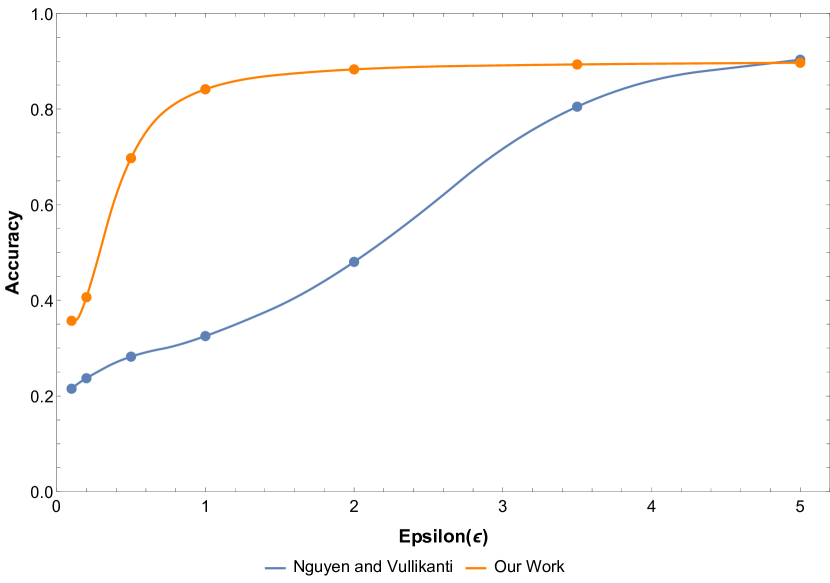
(a) ca-Astro Network

(b) ca-GrQc Network

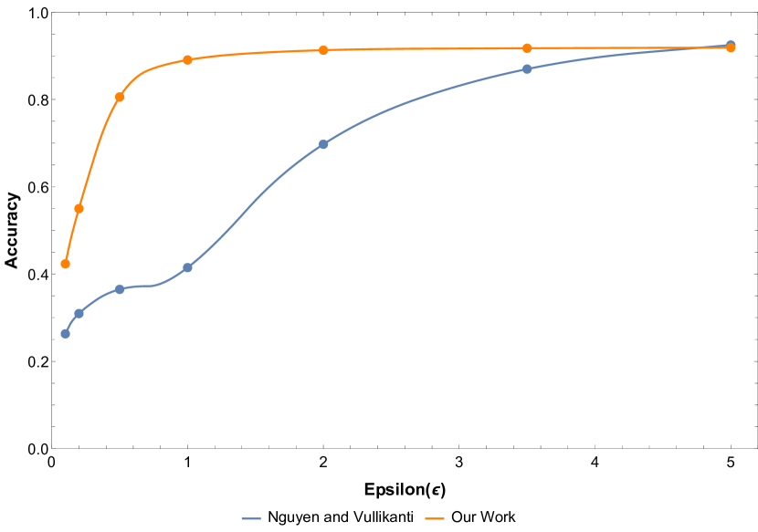
(c) musae DE Network

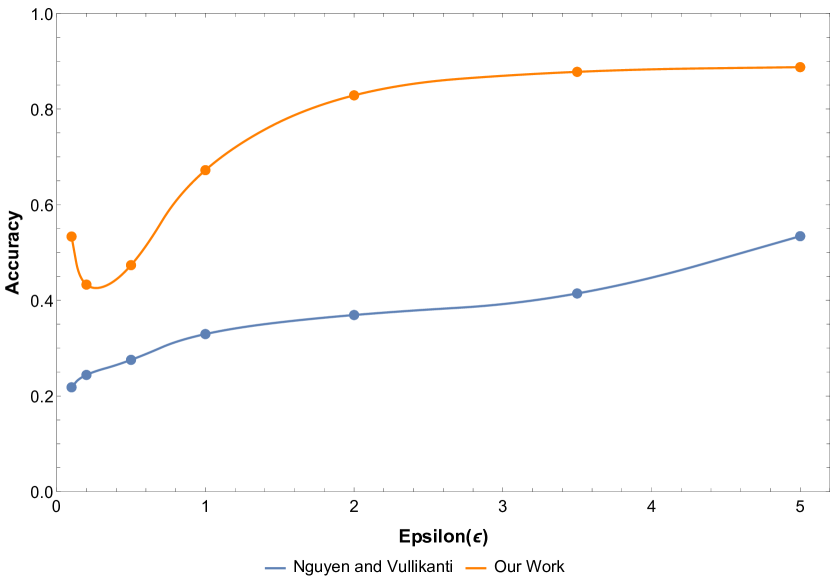
(d) musae ENGB Network

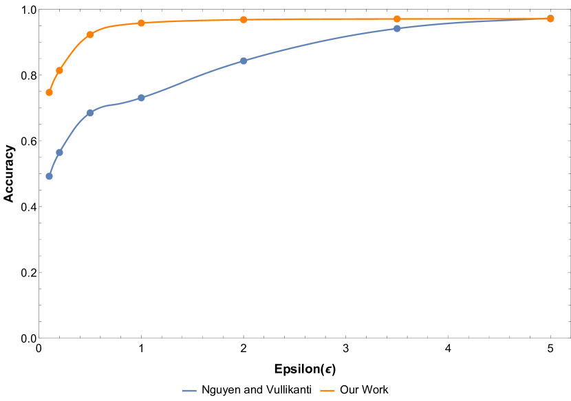
(e) socfb-Amherst41 Network

(f) socfb-Auburn71 Network

Figure 1: Accuracy of our linear-time algorithm as well as the accuracy of the Nguyen and Vullikanti [27]. The orange line shows the accuracy of our proposed algorithm, and the blue line shows the accuracy of Nguyen and Vullikanti.

As mentioned, the algorithm in Section 3.1 takes $O(m+n\log n)$ time. We suggest an improved version that runs in linear time, inspired by a trick suggested by Charikar [7].

Observe that $\bigl{|}\min_{v\in S_{t+1}}|E(v,S_{t+1})|-\min_{v\in S_{t}}|E(v,S_{t})|\bigr{|}\leq 1$. Our algorithm is maintaining a noisy estimate $D(v)-{\sf PSum}(v)$ of $|E(v,S_{t})|$ for all residual vertices $v$. As we discussed, all estimates have at most $O(\frac{1}{\epsilon}\log^{2.5}n\log\frac{1}{\sigma})$ error with $1-\sigma$ probability. Henceforth let $C$ be a sufficiently large constant, and let ${\sf err}:=\frac{C}{\epsilon}\log^{2.5}n\log\frac{1}{\sigma}$. We can discretize the value of $D(v)-{\sf PSum}(v)$ into $B:=\lceil n/{\sf err}+1\rceil$ buckets. The $i$-th bucket will contain values from the range $[(i-1)\cdot{\sf err}-{\sf err}/2,(i-1)\cdot{\sf err}+{\sf err}/2]$. We can now maintain a data structure such that each vertex is placed in the right bucket depending on the current estimate $D(v)-{\sf PSum}(v)$. Inside each bucket, we maintain a linked list of vertices. We also maintain an array such that each vertex stores the bucket it currently belongs to, as well as its pointer in the corresponding linked list.

With this idea, we can modify the algorithm in Section 3.1 into a variant that runs in linear time.

Data : Let $G:=(V,E)$ be the input graph. Let $\epsilon_{0}=\epsilon_{1}=\epsilon_{2}=\epsilon^{\prime}=\epsilon/4$. Let ${\sf T}:=\frac{C}{\epsilon}\log n\log\frac{1}{\sigma}$ for a suitably large constant $C$.

Initialization : Run the initialization steps of Algorithm 1 in Section 3.1, and moreover, place all vertices in the right bucket. Recall that each vertex stores a pointer to where it resides in the linked list of its bucket. Initially, let $\mathit{idx}=1$. We may assume that the (imaginary) 0-th bucket is always empty.

1:  Let $S:=V$ and $d_{\rm max}:=0$. Repeat the following until $S$ is empty:

1. Let $\mathit{idx}^{\prime}$ be the bucket from which a vertex is removed in the previous time step. Check whether each bucket $\mathit{idx}^{\prime}-1,\mathit{idx}^{\prime}$, $\cdots$ is non-empty, and let $\mathit{idx}$ be the smallest non-empty bucket among these. Let $v$ be an arbitrary vertex from this bucket $\mathit{idx}$. Remove $v$ from the bucket.

2. If $d_{\rm max}<D(v)-{\sf PSum}(v)$, then update $d_{\rm max}:=D(v)-{\sf PSum}(v)$ and let $S^{*}:=S$.

3. Remove $v$ from $S$.

4. For each $u\in S$ such that $(u,v)\in E$: let ${\sf Cnt}(u):={\sf Cnt}(u)+1$.

5. For each $u\in S$, if ${\sf Cnt}(u)+{\mathcal{E}}(u)+{\mathcal{N}}>{\sf T}$ where ${\mathcal{N}}:={\sf Geom}(e^{\epsilon_{2}})$ denotes a fresh noise:

   // This line is executed efficiently using the same data structure as mentioned in Section 3.1.

   • Input ${\sf Cnt}(u)$ to ${\sf PSum}(u)$;

   • Based on the updated value $D(u)-{\sf PSum}(u)$, relocate $u$ to a new bucket if necessary;

   • Reset ${\sf Cnt}(u):=0$, and resample a fresh ${\mathcal{E}}(u):={\sf Geom}(e^{\epsilon_{2}})$.

2:  return  $S^{*}$ and $d^{*}:=\min\left(\frac{E(S^{*})+{\sf Geom}(\exp({\epsilon^{\prime}}))}{|S^{*}|},|S^{*}|\right)$.

Algorithm 2 Differentially Private Densest Subgraph - Linear-Time Variant.

Theorem 4.1 (Linear-time variant).

The above algorithm satisfies $\epsilon$-DP and moreover, it achieves $(2,O(\frac{1}{\epsilon}\cdot\log^{2.5}n\cdot\log\frac{1}{\sigma}))$-approximation with probability $1-\sigma$. The algorithm completes in time $O(n+m)$ with $1-\exp(-\Omega(m))$ probability where $n=|V|$ and $m=|E|$.

5 Empirical Results

In this section, we analyze our differentially private algorithm experimentally on real-world datasets and compare it to Charikar’s algorithm and other DP algorithms for the densest subgraph problem. In our experiments, We use Charikar’s algorithm as a non-differential private baseline. Table 1 shows the 6 different networks that we used to evaluate the performance of our algorithm. For a graph $G$, let $S_{c}$ be the subgraph returned by Charikar’s algorithm. We measure the accuracy of a DP algorithm as $\frac{d_{G}(S^{*})}{d_{G}(S_{c})}$ where $S^{*}$ is the subgraph returned by the DP algorithm. In other words, we measure the accuracy of the algorithms based on their relative performance in comparison to Charikar’s algorithm.

Network	Nodes	Edges	Baseline Solution	Description
ca-Astro [25]	18771	198050	29.554	Collaboration net. arXiv Astro Phy.
ca-GrQc [25]	5241	14484	22.3913	Collaboration net. arXiv General Rel.
musae DE [25]	9498	153138	39.0157	Social net. of Twitch (DE)
musae ENGB [25]	7126	35324	11.9295	Social net. of Twitch (GB)
socfb-Amherst41 [29]	2235	90954	54.5489	Social net. of Facebook (Amherst)
socfb-Auburn71 [29]	18448	973918	84.9551	Social net. of Facebook (Auburn)

Table 1: General statistics of networks

Figure 1 shows the accuracy of our linear-time algorithm as well as the accuracy of the $(\epsilon,\delta)$-DP algorithm proposed by Nguyen and Vullikanti [27]. In our experiments, we have set the parameter $\sigma$ equal to $2^{-30}\approx 10^{-9}$ for our algorithm. We have also set $\delta=10^{-9}$ for the $(\epsilon,\delta)$-DP algorithm proposed by Nguyen and Vullikanti. As it is shown in the figure, our proposed algorithm finds a much more accurate solution when $\epsilon$ is small. However, it achieves almost the same accuracy for large choices of $\epsilon$. Note that we have used SEQDENSEDP algorithm to measure the accuracy of the work of Nguyen and Vullikanti which has better accuracy than their parallel algorithms [27].

We also study the running time linear time algorithm and compare it with the running time of SEQDENSEDP algorithm proposed by Nguyen and Vullikanti. Table 2 shows the average running time of the algorithms where the average is taken over 100 trials. Our experimental results show that in the RAM model, our linear time algorithm is much faster than the SEQDENSEDP algorithm. In fact, our linear time algorithm is around 100 times faster than the $(\epsilon,\delta)$-DP algorithm of Nguyen and Vullikanti.

Network	Our work	Nguyen and Vullikanti
ca-Astro	0.069	12.48
ca-GrQc	0.003	0.96
musae DE	0.034	3.36
musae ENGB	0.007	1.8
socfb-Amherst41	$<$0.001	0.21
socfb-Auburn71	0.137	12.24

Table 2: Running time of DP algorithms. All running times are reported in seconds.

Appendix A Failed Naïve Approaches

A standard technique for attaining differential privacy is to add noise to the answer calibrated to the global sensitivity of the function being computed [8]. We argue that this approach fails to give meaningful utility since the densest subgraph problem has high global sensitivity.

Reporting the densest subgraph has high global sensitivity.

The densest subgraph problem has high global sensitivity if we require that the algorithm outputs the set of vertices that form a dense subgraph. For example, one can easily construct a family of graphs $G$ with $n$ vertices, and satisfying the following properties:

• $G$ contains two disjoint sets of vertices $S$ and $S^{\prime}$ of densities $d$ and $d^{\prime}$ respectively. There are no edges between $S$ and $S^{\prime}$.

• The densest subgraph of $S$ is $S$ itself; and the densest subgraph of $S^{\prime}$ is $S^{\prime}$ itself. Furthermore, $d<d^{\prime}<d+1/|S^{\prime}|$.

This means that the densest subgraph of $G$ is $S^{\prime}$; however, if we remove one edge from $S^{\prime}$, the densest subgraph of the resulting graph would become $S$. Therefore, the ordinary approach of perturbing the output with noise roughly proportional to global sensitivity [8] does not apply.

Randomized response gives poor utility.

A naïve approach for solving the DP densest subgraph problem is to rely on randomized response [37, 11, 36] where we use $G=(V,E)$ to denote the original graph given as input:

1. First, generate a rerandomized graph $\widetilde{G}$ as follows: for each $(i,j)\in V^{2}$ and $i<j$, flip the existence of the edge $(i,j)$ with probability $p:=\frac{1}{1+e^{\epsilon}}$.

2. Then, run an exact densest subgraph algorithm on the rerandomized graph $\widetilde{G}$. Output the densest subgraph $S^{*}\subseteq V$ found.

3. Output $d^{*}:=(|E(S^{*})|+{\sf Geom}(e^{\epsilon}))/|S^{*}|$ as an estimate of $d(G)$.

It is not hard to show that the above algorithm satisfies $2\epsilon$-DP, However, the algorithm fails to give a good approximation. To understand why, consider the following example — henceforth we will use $d^{G}(\cdot)$ and $d^{\widetilde{G}}(\cdot)$ to denote the density of a subset of vertices in the original graph $G$ and the rerandomized graph $\widetilde{G}$, respectively. Suppose that $\epsilon=1$ and thus $p=\Theta(1)$. Consider some graph $G=(V,E)$, in which the true densest subgraph $S$ is a clique of size $\sqrt{n}$, and therefore $d(G)=O\big{(}\sqrt{n}\big{)}$. Moreover, suppose that all vertices not in $S$ do not have any edges in $G$. One can show that for any fixed subset $U\subseteq V$ of size at least $\frac{n}{\log^{2}n}$, with $1-o(1)$ probability, $d^{\widetilde{G}}(U)\in[p\cdot|U|/2,2p\cdot|U|]$. Thus with $1-o(1)$ probability, the naïve algorithm will report a large subgraph $U^{*}\approx V$ containing almost all the vertices. However, when $U^{*}\approx V$, the true density $d^{G}(U^{*})=O(1)$ which is a $O(\sqrt{n})$ factor smaller than the true answer $d(G)$. In other words, the reported set $U^{*}$ is not a good approximation of the densest subgraph of $G$.

Appendix B Deferred Proofs for our Quasilinear-Time Scheme

B.1 Deferred Proofs of Differential Privacy

Below, we prove Theorem 3.1.

Fix two arbitrary neighboring graphs $G$ and $\widetilde{G}$ that differ in only one edge. In the proof below, we use the notation $\Pr[\cdot]$ to denote the probability when $G$ is used as the input, and we the notation $\widetilde{\Pr}[\cdot]$ to denote the probability when $\widetilde{G}$ is used as input. In our algorithm, every time a vertex is removed from the residual set $S$, we call it a time step denoted $t$. Let $U_{t}$ be the set of vertices whose ${\sf PSum}$ instance is updated during time step $t$. For a vertex $u\in U_{t}$, let $\Sigma_{t}(u)$ be the new output of ${\sf PSum}(u)$ after the update. Henceforth, we use the notation ${\sf pre}_{t}^{u}$ to denote the time steps up to $t$ (inclusive) in which ${\sf PSum}(u)$ is updated, the increment passed as input to ${\sf PSum}(u)$ during each of these updates, and the new outcome of ${\sf PSum}(u)$ after each update. We use $I_{u}$ to denote the time steps in which $u$ is updated.

For an execution of the algorithm, we define the trace as $\{D(v)\}_{v\in V},\{U_{t},\{\Sigma_{t}(u)\}_{u\in U_{t}}\}_{t}$, where $t$ is different time steps of the algorithm. Note that given the trace, one can uniquely determine the sequence of the vertices removed in the densest subgraph algorithm. Throughout the proof, we fix an arbitrary trace ${\sf tr}=\big{(}\{D(v)\}_{v\in V},\{U_{t},\{\Sigma_{t}(u)\}_{u\in U_{t}}\}_{t}\big{)}$, and we show that $e^{-\epsilon}\cdot\widetilde{\Pr}[{\sf tr}]\leq\Pr[{\sf tr}]\leq e^{\epsilon}\cdot\widetilde{\Pr}[{\sf tr}]$, hence the algorithm is $\epsilon$-DP.

First, consider when $G$ is the input. Let ${\sf pre}_{0}:=\{D(v)\}_{v\in V}$ and for $t>0$, let ${\sf pre}_{t}:=({\sf pre}_{t-1},U_{t},\{\Sigma_{t}(u)\}_{u\in U_{t}})$. We have the following:

$$\Pr[\{D(v)\}_{v\in V},\{U_{t},\{\Sigma_{t}(u)\}_{u\in U_{t}}\}_{t}]$$

$$= \Pr[{\sf pre}_{0}]\cdot\prod_{t>0}\bigg{(}\Pr[U_{t}|{\sf pre}_{t-1}]\cdot$$

$$\ \ \quad\qquad\cdot\prod_{u\in U_{t}}\Pr\left[{\sf PSum}(u)\text{ outputs }\Sigma_{t}(u)\text{ on new input }{\sf Cnt}^{G}_{t}(u)\left|({\sf pre}_{t-1},U_{t})\right.\right]\bigg{)}$$

$$= \Pr[{\sf pre}_{0}]\cdot\prod_{t>0}\bigg{(}\Pr[U_{t}|{\sf pre}_{t-1}]$$

$$\ \ \qquad\quad\cdot\prod_{u\in U_{t}}\Pr\left[{\sf PSum}(u)\text{ outputs }\Sigma_{t}(u)\text{ on new input }{\sf Cnt}^{G}_{t}(u)\left|{\sf pre}_{t-1}^{u}\right.\right]\bigg{)}$$

$$= \Pr[{\sf pre}_{0}]\cdot\prod_{t>0}\Pr[U_{t}|{\sf pre}_{t-1}]\cdot\prod_{u\in V}\Pr\left[{\sf PSum}(u)\text{ outputs }\{\Sigma_{t}(u)\}_{t\in I_{u}}\text{ on updates }\{{\sf Cnt}^{G}_{t}(u)\}_{t\in I_{u}}\right]$$

Similarly, we have that

$$\widetilde{\Pr}[\{D(v)\}_{v\in V},\left\{U_{t},\{\Sigma_{t}(u)\}_{u\in U_{t}}\right\}_{t}]$$

$$= \widetilde{\Pr}[{\sf pre}_{0}]\cdot\prod_{t>0}\widetilde{\Pr}[U_{t}|{\sf pre}_{t-1}]\cdot\prod_{u\in V}\widetilde{\Pr}\left[{\sf PSum}(u)\text{ outputs }\{\Sigma_{t}(u)\}_{t\in I_{u}}\text{ on updates }\{{\sf Cnt}^{\widetilde{G}}_{t}(u)\}_{t\in I_{u}}\right]$$

Claim B.1.

$e^{-\epsilon_{0}}\cdot{\Pr[{\sf pre}_{0}]}\leq{\widetilde{\Pr}[{\sf pre}_{0}]}\leq e^{\epsilon_{0}}\cdot{\Pr[{\sf pre}_{0}]}$

Proof. Observe that $G$ and $\widetilde{G}$ differ in at most one edge, and the (non)-existence of every edge affects the degree of at most two vertices. The claim therefore follows from Fact 1. $\Box$

Claim B.2.

$$e^{-\epsilon_{2}}\cdot\prod_{t>0}{\Pr}[U_{t}|{\sf pre}_{t-1}] \leq\prod_{t>0}\widetilde{\Pr}[U_{t}|{\sf pre}_{t-1}]\leq e^{\epsilon_{2}}\cdot\prod_{t>0}{\Pr}[U_{t}|{\sf pre}_{t-1}]$$

Proof. Recall that two graphs $G$ and $\widetilde{G}$ differ in only one edge. Let $e=\{i,j\}$ be this edge, then we can assume w.l.o.g. that $e\in G$ and $e\notin\widetilde{G}$. Now consider the trace $\{D(v)\}_{v\in V},\{U_{t},\{\Sigma_{t}(u)\}_{u\in U_{t}}\}_{t}$. As we discussed earlier given the trace, we can uniquely determine the sequence of the vertices removed in Step 4 of the algorithm. Let $t^{\prime}$ be the first time step that the algorithm removes one of the vertices $i$ or $j$. By symmetry, we can assume that this vertex is $i$, i.e., $i\in U_{t^{\prime}}$.

Assuming that the algorithm has the same set of noisy degrees $\{D(v)\}_{v\in V}$ at the beginning for both graphs $G$ and $\widetilde{G}$, the algorithm does not see any difference between $G$ and $\tilde{G}$ until it reaches time $t^{\prime}$. This is because for every vertex $v$ that the algorithm removes before time $t^{\prime}$, this vertex has the same set of neighbors in both $G$ and $\widetilde{G}$. Therefore,

$$\prod_{0<t<t^{\prime}}{\Pr}[U_{t}|{\sf pre}_{t-1}]=\prod_{0<t<t^{\prime}}\widetilde{\Pr}[U_{t}|{\sf pre}_{t-1}]\,.$$ (1)

Note that the equality above follows from the fact that given ${\sf pre}_{0}$, the algorithm has the same set of noisy degrees $\{D(v)\}_{v\in V}$ for both $G$ and $\widetilde{G}$.

Consider the time step $t^{\prime}$ where the algorithm removes $i$ from $S$. When we run the algorithm on $G$, vertex $j$ is a neighbor of $i$. Thus, the algorithm increases the ${\sf Cnt}(j)$ in this time step. However, this is not the case in $\widetilde{G}$, and the ${\sf Cnt}(j)$ remains the same when we run the algorithm on $\widetilde{G}$. We consider two cases for the rest of the proof.

• Case 1: The first case is when $j\notin U_{t}$ for any $t\geq t^{\prime}$. This means that the algorithm never updates the ${\sf PSum}(j)$ after the step $t^{\prime}$. Let $t^{\prime\prime}$ be the time step where the algorithm removes $j$ from $S$ in Step 4 of the algorithm. It is easy to see that given the trace of the algorithm, we can uniquely determine $t^{\prime\prime}$. We then have,

  $$\prod_{t^{\prime}\leq t\leq t^{\prime\prime}}{\Pr}[U_{t}|{\sf pre}_{t-1}] =\prod_{t^{\prime}\leq t\leq t^{\prime\prime}}\bigg{(}\prod_{u\in U_{t}}{\Pr}[u\in U_{t}|{\sf pre}_{t-1}]\cdot\prod_{u\notin U_{t}}{\Pr}[u\notin U_{t}|{\sf pre}_{t-1}]\bigg{)}$$

  $$=\prod_{u\in V}\bigg{(}\prod_{t\in[t^{\prime},t^{\prime\prime}]\cap I_{u}}{\Pr}[u\in U_{t}|{\sf pre}_{t-1}]\cdot\prod_{t\in[t^{\prime},t^{\prime\prime}]-I_{u}}{\Pr}[u\notin U_{t}|{\sf pre}_{t-1}]\bigg{)}\,.$$ (2)

  Similarly, for the graph $\widetilde{G}$, we have

  $$\prod_{t^{\prime}\leq t\leq t^{\prime\prime}}\widetilde{\Pr}[U_{t}|{\sf pre}_{t-1}] =\prod_{u\in V}\bigg{(}\prod_{t\in[t^{\prime},t^{\prime\prime}]\cap I_{u}}\widetilde{\Pr}[u\in U_{t}|{\sf pre}_{t-1}]\cdot\prod_{t\in[t^{\prime},t^{\prime\prime}]-I_{u}}\widetilde{\Pr}[u\notin U_{t}|{\sf pre}_{t-1}]\bigg{)}\,.$$ (3)

  In order to complete the proof of this case, we first claim that for every vertex $u\neq j$, we have

  $$\prod_{t\in[t^{\prime},t^{\prime\prime}]\cap I_{u}}{\Pr}[u\in U_{t}|{\sf pre}_{t-1}]\cdot\prod_{t\in[t^{\prime},t^{\prime\prime}]-I_{u}}{\Pr}[u\notin U_{t}|{\sf pre}_{t-1}]$$

  $$=\prod_{t\in[t^{\prime},t^{\prime\prime}]\cap I_{u}}\widetilde{\Pr}[u\in U_{t}|{\sf pre}_{t-1}]\cdot\prod_{t\in[t^{\prime},t^{\prime\prime}]-I_{u}}\widetilde{\Pr}[u\notin U_{t}|{\sf pre}_{t-1}]\,.$$ (4)

  The claim clearly holds for every vertex $u\neq i,j$, since $u$ has exactly the same set of neighbors in both $G$ and $\widetilde{G}$. Therefore, given ${\sf pre}_{t-1}$ we have ${\sf Cnt}^{G}_{t}(u)={\sf Cnt}^{\widetilde{G}}_{t}(u)$, thus the claim holds. Also, considering the vertex $i$, the algorithm removes $i$ from $S$ at the time step $t^{\prime}$, and it never updates the prefix sum for $i$ after that. Therefore ${\Pr}[i\in U_{t}|{\sf pre}_{t-1}]=\widetilde{\Pr}[i\in U_{t}|{\sf pre}_{t-1}]=0$ for any $t\geq t^{\prime}$. Similarly, we have ${\Pr}[i\notin U_{t}|{\sf pre}_{t-1}]=\widetilde{\Pr}[i\notin U_{t}|{\sf pre}_{t-1}]=1$ for any $t\geq t^{\prime}$ which implies our claim for the vertex $i$. We now give the following bound for vertex $j$.

  Claim B.3.

  For Case 1, let $p=\prod_{t\in[t^{\prime},t^{\prime\prime}]\cap I_{j}}{\Pr}[j\in U_{t}|{\sf pre}_{t-1}]\cdot\prod_{t\in[t^{\prime},t^{\prime\prime}]-I_{j}}{\Pr}[j\notin U_{t}|{\sf pre}_{t-1}]$ and $\widetilde{p}=\prod_{t\in[t^{\prime},t^{\prime\prime}]\cap I_{j}}\widetilde{\Pr}[j\in U_{t}|{\sf pre}_{t-1}]\cdot\prod_{t\in[t^{\prime},t^{\prime\prime}]-I_{j}}\widetilde{\Pr}[j\notin U_{t}|{\sf pre}_{t-1}]$, we then have $e^{-\epsilon_{2}}\widetilde{p}\leq p\leq e^{\epsilon_{2}}\widetilde{p}$.

  Proof. Recall that we are assuming that $j\notin U_{t}$ for any $t\geq t^{\prime}$. Therefore, $[t^{\prime},t^{\prime\prime}]\cap I_{j}=\emptyset$, and we have

  $$\prod_{t\in[t^{\prime},t^{\prime\prime}]\cap I_{j}}{\Pr}[j\in U_{t}|{\sf pre}_{t-1}]\cdot\prod_{t\in[t^{\prime},t^{\prime\prime}]-I_{j}}{\Pr}[j\notin U_{t}|{\sf pre}_{t-1}]={\Pr}[j\notin\cup_{t^{\prime}\leq t\leq t^{\prime\prime}}U_{t}|{\sf pre}_{t^{\prime}-1}]\,.$$

  Similarly, we have

  $$\prod_{t\in[t^{\prime},t^{\prime\prime}]\cap I_{j}}\widetilde{\Pr}[j\in U_{t}|{\sf pre}_{t-1}]\cdot\prod_{t\in[t^{\prime},t^{\prime\prime}]-I_{j}}\widetilde{\Pr}[j\notin U_{t}|{\sf pre}_{t-1}]=\widetilde{\Pr}[j\notin\cup_{t^{\prime}\leq t\leq t^{\prime\prime}}U_{t}|{\sf pre}_{t^{\prime}-1}]\,.$$

  Now considering the vertex $j$, the expression ${\Pr}[j\notin\cup_{t^{\prime}\leq t\leq t^{\prime\prime}}U_{t}|{\sf pre}_{t^{\prime}-1}]$ (or $\widetilde{\Pr}[j\notin\cup_{t^{\prime}\leq t\leq t^{\prime\prime}}U_{t}|{\sf pre}_{t^{\prime}-1}]$) can be equivalently thought as the following. For every time step $t^{\prime}\leq t\leq t^{\prime\prime}$, compute the noisy counter ${\sf Cnt}(j)+{\mathcal{N}}$ and compare it with the noisy threshold ${\sf T}-{\mathcal{E}}(j)$, where ${\mathcal{N}}$ is a fresh random noise, and ${\mathcal{E}}(j)$ was chosen the last time ${\sf Cnt}(j)$ was reset to 0. We want to know what is the probability that for all of $t^{\prime}\leq t\leq t^{\prime\prime}$, ${\sf Cnt}(j)+{\mathcal{N}}$ never exceeds the threshold ${\sf T}-{\mathcal{E}}(j)$. This random process is identical to the sparse vector algorithm (see page 57, Algorithm 1 of [11]), applied to the following database and sequence of queries, with the privacy budget $\epsilon_{2}$. Specifically, the database here is a sequence of boolean values that represent whether $j$ is connected to the vertex being removed in steps $t\in[t^{\prime},t^{\prime\prime}]$. The sequence of queries is whether the prefix sum of the database in each time step exceeds ${\sf T}$. Note that for $G$ and $\widetilde{G}$ the two databases defined above differ only in one position, i.e., the bit in time step $t^{\prime}$ when $i$ is removed. Moreover, all the prefix sums have sensitity $1$. The proof of the sparse vector technique immediately gives us the following (see Theorem 3.23 of [11]):

  $$e^{-\epsilon_{2}}\cdot\widetilde{\Pr}[j\notin\cup_{t^{\prime}\leq t\leq t^{\prime\prime}}U_{t}|{\sf pre}_{t^{\prime}-1}]\leq{\Pr} [j\notin\cup_{t^{\prime}\leq t\leq t^{\prime\prime}}U_{t}|{\sf pre}_{t^{\prime}-1}]$$

  $$\leq e^{\epsilon_{2}}\cdot\widetilde{\Pr}[j\notin\cup_{t^{\prime}\leq t\leq t^{\prime\prime}}U_{t}|{\sf pre}_{t^{\prime}-1}]\,.$$

  $\Box$

  Considering any time step $t>t^{\prime\prime}$, the algorithm has removed both vertices $i$ and $j$, and it does not see any difference between $G$ and $\widetilde{G}$. Thus,

  $$\prod_{t^{\prime\prime}<t}{\Pr}[U_{t}|{\sf pre}_{t-1}]=\prod_{t^{\prime\prime}<t}\widetilde{\Pr}[U_{t}|{\sf pre}_{t-1}]\,.$$

  The equality above along with equalities (1), (• ‣ B.1) and also Claim B.3 implies Claim B.2 for this case.

• Case 2: The second case is when $j\in U_{t}$ for some $t\geq t^{\prime}$. Let $t^{\prime\prime}\geq t^{\prime}$ be the smallest index such that $j\in U_{t^{\prime\prime}}$. It is easy to verify that equations (• ‣ B.1) and (3) still hold in Case 2. Also, Equation (• ‣ B.1) holds for every vertex $u\neq j$. We now give the following bound for vertex $j$.

  Claim B.4.

  For Case 2, let $p=\prod_{t\in[t^{\prime},t^{\prime\prime}]\cap I_{j}}{\Pr}[j\in U_{t}|{\sf pre}_{t-1}]\cdot\prod_{t\in[t^{\prime},t^{\prime\prime}]-I_{j}}{\Pr}[j\notin U_{t}|{\sf pre}_{t-1}]$ and $\widetilde{p}=\prod_{t\in[t^{\prime},t^{\prime\prime}]\cap I_{j}}\widetilde{\Pr}[j\in U_{t}|{\sf pre}_{t-1}]\cdot\prod_{t\in[t^{\prime},t^{\prime\prime}]-I_{j}}\widetilde{\Pr}[j\notin U_{t}|{\sf pre}_{t-1}]$, we then have $e^{-\epsilon_{2}}\widetilde{p}\leq p\leq e^{\epsilon_{2}}\widetilde{p}$.

  Proof. Recall that we are assuming that $j\in U_{t^{\prime\prime}}$ and $j\notin U_{t}$ for any $t^{\prime}\leq t<t^{\prime\prime}$. Therefore, $[t^{\prime},t^{\prime\prime}]\cap I_{j}=\{t^{\prime\prime}\}$, and we have

  $$\prod_{t\in[t^{\prime},t^{\prime\prime}]\cap I_{j}}{\Pr}[j\in U_{t}|{\sf pre}_{t-1}]\cdot\prod_{t\in[t^{\prime},t^{\prime\prime}]-I_{j}}{\Pr}[j\notin U_{t}|{\sf pre}_{t-1}]$$

  $$={\Pr}[j\in U_{t^{\prime\prime}}|{\sf pre}_{t^{\prime\prime}-1}]\cdot{\Pr}[j\notin\cup_{t^{\prime}\leq t<t^{\prime\prime}}U_{t}|{\sf pre}_{t^{\prime}-1}]\quad\ \ (\text{henceforth denoted }{p})\,.$$

  Similarly, we have

  $$\prod_{t\in[t^{\prime},t^{\prime\prime}]\cap I_{j}}\widetilde{\Pr}[j\in U_{t}|{\sf pre}_{t-1}]\cdot\prod_{t\in[t^{\prime},t^{\prime\prime}]-I_{j}}\widetilde{\Pr}[j\notin U_{t}|{\sf pre}_{t-1}]$$

  $$=\widetilde{\Pr}[j\in U_{t^{\prime\prime}}|{\sf pre}_{t^{\prime\prime}-1}]\cdot\widetilde{\Pr}[j\notin\cup_{t^{\prime}\leq t<t^{\prime\prime}}U_{t}|{\sf pre}_{t^{\prime}-1}]\quad\ \ (\text{henceforth denoted }\widetilde{p})\,.$$

  The expressions $p$ or $\widetilde{p}$ are equivalent to the following. For every time step $t^{\prime}\leq t\leq t^{\prime\prime}$, the algorithm computes the noisy counter ${\sf Cnt}(j)+{\mathcal{N}}$ and compares it to the noisy threshold ${\sf T}-{\mathcal{E}}(j)$. We want to know what is the probability that for all of $t^{\prime}\leq t<t^{\prime\prime}$, ${\sf Cnt}(j)+{\mathcal{N}}$ does not exceed threshold ${\sf T}-{\mathcal{E}}(j)$, but finally in time $t^{\prime\prime}$, ${\sf Cnt}(j)+{\mathcal{N}}$ indeed exceeds threshold ${\sf T}-{\mathcal{E}}(j)$. Similar to what we discussed in Claim B.3, we can directly apply the analysis of the sparse vector technique here, and obtain that $e^{-\epsilon_{2}}\cdot\widetilde{p}\leq p\leq e^{\epsilon_{2}}\cdot\widetilde{p}$.

  $\Box$

  Considering any time step $t>t^{\prime\prime}$, the algorithm has removed vertices $i$ and $j$, and the induced subgraph between the vertices in $S$ is exactly the same for both graphs $G$ and $\widetilde{G}$. The algorithm also resets the counters ${\sf Cnt}^{G}(j)$ and ${\sf Cnt}^{\widetilde{G}}(j)$ at the time step $t^{\prime\prime}$. Furthermore, the ${\sf PSum}$ values are exactly the same for $G$ and $\widetilde{G}$ conditioning on ${\sf pre}_{t^{\prime\prime}}$. Thus, the algorithm does not see any difference between $G$ and $\widetilde{G}$ after the time step $t^{\prime\prime}$ and we have

  $$\prod_{t^{\prime\prime}<t}{\Pr}[U_{t}|{\sf pre}_{t-1}]=\prod_{t^{\prime\prime}<t}\widetilde{\Pr}[U_{t}|{\sf pre}_{t-1}]\,.$$

  The equality above along with equalities (1), (• ‣ B.1) and also Claim B.4 implies Claim B.2 for this case.

This completes the proof for both Case 1 and Case 2 and proves Claim B.2. $\Box$

Claim B.5.

Let ${p}:=\prod_{u\in V}{\Pr}\left[{\sf PSum}(u)\text{ outputs }\{\Sigma_{t}(u)\}_{t\in I^{u}}\text{ on updates }\{{\sf Cnt}^{{G}}_{t}(u)\}_{t\in I^{u}}\right]$ and let $\widetilde{p}:=\prod_{u\in V}\widetilde{\Pr}\left[{\sf PSum}(u)\text{ outputs }\{\Sigma_{t}(u)\}_{t\in I^{u}}\text{ on updates }\{{\sf Cnt}^{\widetilde{G}}_{t}(u)\}_{t\in I^{u}}\right]$. It must be that $e^{-\epsilon_{1}}p\leq\widetilde{p}\leq e^{\epsilon_{1}}p$.

Proof. Since $G$ and $\widetilde{G}$ are neighboring, there is at most one $(u,t)$ pair where $t\in I_{u}$ such that ${\sf Cnt}^{\widetilde{G}}_{t}(u)$ and ${\sf Cnt}^{{G}}_{t}(u)$ differ by 1. For all other $(u,t)$ pair where $t\in I_{u}$, ${\sf Cnt}^{\widetilde{G}}_{t}(u)$ and ${\sf Cnt}^{{G}}_{t}(u)$ must be the same. The claim therefore follows from the $\epsilon_{1}$-DP of the prefix sum mechanism.

Proof of Theorem 3.1.

Let $S^{*}$ be the subgraph output by the algorithm. Observe that $S^{*}$ is uniquely determined by trace $\{D(v)\}_{v\in V},\left\{U_{t},\allowbreak\{\Sigma_{t}(u)\}_{u\in U_{t}}\right\}_{t}$. Therefore, given Claims B.1, B.2, and B.5, we conclude that for any $S^{*}$, $e^{-(\epsilon_{0}+\epsilon_{1}+\epsilon_{2})}\cdot\Pr[S^{*}]\leq\widetilde{\Pr}[S^{*}]\leq e^{\epsilon_{0}+\epsilon_{1}+\epsilon_{2}}\cdot\Pr[S^{*}]$. Besides $S^{*}$, the algorithm also needs to output $d^{*}$. Since $G$ and $\widetilde{G}$ differ in at most one edge, and due to the distribution of the noise in computing $d^{*}$, it follows that for any $d^{*}$ and $S^{*}$,

$$e^{-\epsilon^{\prime}}\Pr[d^{*}|S^{*}]\leq\widetilde{\Pr}[d^{*}|S^{*}]\leq e^{\epsilon^{\prime}}\Pr[d^{*}|S^{*}]$$

Therefore, for any $S^{*}$ and $d^{*}$, we have that $e^{-(\epsilon_{0}+\epsilon_{1}+\epsilon_{2}+\epsilon^{\prime})}\cdot\Pr[S^{*},d^{*}]\leq\widetilde{\Pr}[S^{*},d^{*}]\leq e^{\epsilon_{0}+\epsilon_{1}+\epsilon_{2}+\epsilon^{\prime}}\cdot\Pr[S^{*},d^{*}]$. $\Box$

B.2 Deferred Proofs of Utility

In this section, we prove Theorem 3.2.

To prove Theorem 3.2, we will need to use the following lemma proven by Charikar [7].

Lemma B.6 (Upper bound on $d(G)$ [7]).

Let $G:=(V,E)$ be an undirected graph, and suppose that we arbitrarily assign an orientation to each edge. Let $d_{\rm max}$ be the maximum number of edges oriented towards any vertex. Then, it must be that $d(G)\leq d_{\rm max}$.

Proof. of Theorem 3.2

Claim B.7.

With $1-0.1\sigma$ probability, the following holds throughout the algorithm: at the beginning of every time step, let $S$ be the residual set, and let $v\in S$; then,

$$\bigl{|}D(v)-{\sf PSum}(v)-|E(v,S)|\bigr{|}\leq O\left(\frac{1}{\epsilon}\cdot\log^{2.5}n\cdot\log\frac{1}{\sigma}\right)+{\sf T}.$$

Proof. Recall that $\epsilon_{0}=\epsilon_{1}=\epsilon_{2}=\epsilon^{\prime}=\epsilon/4$. For a fixed $v\in V$, by the property of the ${\sf Geom}(e^{\epsilon_{0}/2})$ noise distribution in $D(v)$, with probability $1-\frac{0.1\sigma}{2n}$, $|{\sf deg}(v)-D(v)|<\frac{C}{\epsilon}\cdot\log n\cdot\log\frac{1}{\sigma}$ for some appropriate constant $C$. Taking the union bound over all $v\in V$, with probability $1-0.1\sigma/2$, it holds that for all $v\in V$, $|{\sf deg}(v)-D(v)|<\frac{C}{\epsilon}\cdot\log n\cdot\log\frac{1}{\sigma}$.

By Theorem 2.4, for any $v\in V$ and any fixed time step, with probability $1-\frac{0.1\sigma}{2n^{2}}$, the error of ${\sf PSum}(v)$ for the fixed time step is upper bounded by $O(\frac{1}{\epsilon}\cdot\log^{2.5}n\cdot\log\frac{1}{\sigma})$. Taking a union bound over all time steps, it must be that for any fixed $v$, with probability $1-\frac{0.1\sigma}{2n}$, the error of ${\sf PSum}(v)$ is upper bounded $O(\frac{1}{\epsilon}\cdot\log^{2.5}n\cdot\log\frac{1}{\sigma})$ in all time steps. Taking a union bound over all vertices, it must be that with probability $1-\frac{0.1\sigma}{2}$, the above holds for all vertices.

Recall that we do not update ${\sf PSum}(v)$ in every time step, only when ${\sf Cnt}(v)+{\mathcal{E}}(v)+{\mathcal{N}}$ has exceeded the threshold ${\sf T}$. Further, $E(v,V\backslash S)$ is equal to the true sum of all increments input to ${\sf PSum}(v)$ so far, plus ${\sf Cnt}(v)$. For any fixed ${\mathcal{E}}(v)$, with $1-0.1\sigma/n^{3}$ probability, $|{\mathcal{E}}(v)|\leq O(\frac{1}{\epsilon}\log n\log\frac{1}{\sigma})$. The same holds for each fixed ${\mathcal{N}}$. Therefore, with $1-0.1\sigma$ probability, it must be that any noise ${\mathcal{E}}(v)$ or ${\mathcal{N}}$ generated throughout the algorithm has magnitude at most $O(\frac{1}{\epsilon}\log n\log\frac{1}{\sigma})$. This means with $1-0.1\sigma$ probability, throughout the algorithm and for any $v$, the outstanding counter value ${\sf Cnt}(v)$ that has not been accumulated by ${\sf PSum}(v)$ cannot exceed ${\sf T}+O(\frac{1}{\epsilon}\log n\log\frac{1}{\sigma})$.

Therefore, with probability $1-0.1\sigma$, it must be that at the beginning of every time step, and for every $v\in S$ where $S$ is the current residual set — henceforth, we use ${\sf TruePSum(v)}$ to mean the true prefix sum of all inputs that have been sent to ${\sf PSum}(v)$:

$$\bigl{|}D(v)-{\sf PSum}(v)-|E(v,S)|\bigr{|}$$

$$= \bigl{|}D(v)-{\sf PSum}(v)-({\sf deg}(v)-|E(v,V\backslash S|)\bigr{|}$$

$$\leq \bigl{|}D(v)-{\sf deg}(v)\bigr{|}+\bigl{|}|E(v,V\backslash S|)-{\sf PSum}(v)\bigr{|}$$

$$= \bigl{|}D(v)-{\sf deg}(v)\bigr{|}+\bigl{|}{\sf Cnt}(v)+{\sf TruePSum}(v)-{\sf PSum}(v)\bigr{|}$$

$$\leq \bigl{|}D(v)-{\sf deg}(v)\bigr{|}+\bigl{|}{\sf Cnt}(v)\bigr{|}+\bigl{|}{\sf TruePSum}(v)-{\sf PSum}(v)\bigr{|}$$

$$\leq O\left(\frac{1}{\epsilon}\cdot\log n\cdot\log\frac{1}{\sigma}\right)+{\sf T}+O\left(\frac{1}{\epsilon}\cdot\log n\cdot\log\frac{1}{\sigma}\right)+O\left(\frac{1}{\epsilon}\cdot\log^{2.5}n\cdot\log\frac{1}{\sigma}\right)$$

$$\leq O\left(\frac{1}{\epsilon}\cdot\log^{2.5}n\cdot\log\frac{1}{\sigma}\right)+{\sf T}$$

$\Box$

Claim B.8.

Consider some execution of our algorithm, and let and let ${\sf err}:=\max_{t,v\in S_{t}}\bigl{|}D(v)-{\sf PSum}_{t}(v)-|E(v,S_{t})|\bigr{|}$ where $S_{t}$ denotes the residual set at the beginning of time step $t$, and ${\sf PSum}_{t}(v)$ denotes the output of ${\sf PSum}(v)$ at the beginning of time step $t$. Then, $d(S^{*})\geq(d(G)-4\cdot{\sf err})/2$.

Proof. Fix an arbitrary time step $t$, it holds that $\min_{v\in S_{t}}|E(v,S_{t})|\leq 2|E(S_{t})|/|S_{t}|$. Let $v_{t}\in S_{t}$ be the actual vertex that is removed in time step $t$, i.e., $v_{t}:={\rm arg}\min_{v}(D(v)-{\sf PSum}_{t}(v))$. It therefore holds that $|E(v_{t},S_{t})|-\min_{v\in S_{t}}|E(v,S_{t})|\leq 2\cdot{\sf err}$.

Now, suppose that as a vertex $v_{t}$ gets removed from the residual graph $S_{t}$, all edges $E(v_{t},S_{t})$ are oriented towards $v_{t}$. Observe that the $d_{\rm max}:=\max_{t}(D(v_{t})-{\sf PSum}_{t}(v_{t}))$ value at the end of the algorithm is a good estimate of $\max_{t}(E(v_{t},S_{t}))$. Specifically, $d_{\rm max}\geq\max_{t}(E(v_{t},S_{t}))-2\cdot{\sf err}$. Henceforth let $t^{*}:={\rm arg}\max_{t}(D(v_{t})-{\sf PSum}_{t}(v_{t}))$, and therefore, our algorithm’s output $S^{*}:=S_{t^{*}}$.

By Lemma B.6, it holds that $d(G)\leq\max_{t}(E(v_{t},S_{t}))\leq d_{\rm max}+2\cdot{\sf err}=D(v_{t^{*}})-{\sf PSum}_{t^{*}}(v_{t^{*}})+2\cdot{\sf err}\leq\min_{v\in S_{t^{*}}}|E(v,S_{t^{*}})|+2\cdot{\sf err}+2\cdot{\sf err}=2\cdot{\sf err}\leq 2|E(S_{t^{*}})|/|S_{t^{*}}|+4\cdot{\sf err}=2|E(S^{*})|/|S^{*}|+4\cdot{\sf err}$. In other words, $d(S^{*})\geq(d(G)-4\cdot{\sf err})/2$. $\Box$

Finally, observe that by the definition of $d^{*}$ and due to Fact 1, with probability $1-0.1\sigma$, $|d^{*}-d(S^{*})|\leq O(\frac{1}{\epsilon}\log\frac{1}{\sigma})$. Theorem 3.2 now follows from this fact, as well as Claims B.7 and B.8, and the choice of ${\sf T}$. $\Box$

Appendix C Deferred Proofs for the Linear-Time Algorithm

In this section, we prove Theorem 4.1. The DP proof is the same as Theorem 3.1. For the utility analysis, we may assume that whenever ${\sf PSum}(u)$ is updated from $\Sigma$ to $\Sigma^{\prime}$ for any vertex $u$, it holds that $\Sigma^{\prime}-\Sigma<{\sf err}/2$ where ${\sf err}$ is the discretization parameter used in the bucketing — using the same type of arguments as the proof of Claim B.7, one can show that this indeed holds except with $0.1\sigma$ probability. This means that no vertex $v$’s noisy residual degree $D(v)-{\sf PSum}(v)$ should shrink by more than ${\sf err}/2+1$ in two adjacent time steps, i.e., whenever a vertex $v$ moves buckets, it cannot move left by more than 1 bucket. Therefore, effectively, the only difference between this linear-time variant and the earlier algorithm in Section 3.1 is the following: in this new variant, we do not necessarily pick ${\rm arg}\min_{v}(v,S_{t})$ in every time step $t$. We could pick a vertex $v_{t}$ in time step $t$ such that $|v_{t}-{\rm arg}\min_{v}(v,S_{t})|\leq{\sf err}$. This introduces an additive ${\sf err}$ term in the proof of Theorem 3.2. Due to the choice of ${\sf err}$, and redoing Theorem 3.2 with the extra additive ${\sf err}$ term, we conclude that the above algorithm achieves $(2,O(\frac{1}{\epsilon}\cdot\log^{2.5}n\cdot\log\frac{1}{\sigma}))$-approximation with probability $1-\sigma$.

We now bound the algorithm’s runtime. First, not counting the runtime associated with ${\sf PSum}$ updates, the rest of the algorithm is easily seen to take only $O(n+m)$ time — specifically, the total work spent in Line 1 is at most $O(n)$ due to the same reason as Charika’s non-DP, linear-time algorithm. Due to the runtime of ${\sf PSum}$ stated in Theorem 2.4, to prove the statement about the runtime, it suffices to show that the number of ${\sf PSum}$ updates is upper bounded by $4m$ with probability $\exp(-\Omega(m))$. Consider running the algorithm till it makes exactly $4m$ ${\sf PSum}$ updates — if the algorithm ends before making $4m$ ${\sf PSum}$ updates, we can simply pad it to exactly $4m$ number of ${\sf PSum}$ updates by appending filler ${\sf PSum}$ updates at the end of the algorithm which does not affect the outcome. In this way, there is exactly one noise ${\mathcal{E}}$ associated with each of the $4m$ ${\sf PSum}$ updates. Due to the choice of ${\sf T}$, the probability that each ${\mathcal{E}}$ is greater than ${\sf T}$ is at most $\sigma/n$. Due to the Chernoff bound, the probability that there exist $3m$ or more noises ${\mathcal{E}}$ that are greater than ${\sf T}$ is $\exp(-\Omega(m))$. This means that for $m$ of these ${\sf PSum}$ updates, the true increment input to the ${\sf PSum}$ instance must be at least $1$, and thus one edge must be consumed for each of these $m$ ${\sf PSum}$ updates. In other words, except with $\exp(-\Omega(m))$ probability, the algorithm must have ended after having made $4m$ or fewer ${\sf PSum}$ updates.

Appendix D Lower Bound

Theorem 1.3. Let $\alpha>1$, $\epsilon>0$ be arbitrary constants, $\exp(-n^{0.49})<\sigma<0.000001\cdot\min(1,\epsilon,\exp(-\epsilon))$, and $0\leq\delta\leq\frac{\sigma\epsilon}{\log\frac{1}{4\sigma}}$. Then, there exists a sufficiently small $\beta=\Theta\big{(}\frac{1}{\alpha}\sqrt{\frac{1}{\epsilon}\log\frac{1}{\sigma}}\big{)}$ such that there does not exist an $(\epsilon,\delta)$-DP mechanism that achieves $(\alpha,\beta)$-approximation with $1-\sigma$ probability.

Proof. Suppose there exists an $(\epsilon,\delta)$-DP mechanism denoted $M$ that achieves $(\alpha,\beta)$-approximation with $1-\sigma$ probability, for the parameters stated above. Let $\beta=\frac{1}{100\alpha}\sqrt{\frac{1}{\epsilon}\log\frac{1}{4\sigma}}$. We will reach a contradition below. Thus, no $(\epsilon,\delta)$-DP mechanism can achieve a $(\alpha,\beta)$-approximation.

Consider a graph over $n$ vertices $V:=[n]$. Suppose that a subset $A\subseteq V$ of size $4\alpha\beta+1$ of the vertices form a clique, and there are no other edges in $G$. Therefore, the densest subgraph of $G$ is $A$, and its density is $\frac{|A|-1}{2}$ which is $2\alpha\beta$. Note that for our choices of parameters, we always have $\alpha\beta\geq 1$.

If we run the mechanism $M$ over this graph $G$, we know that with probability $1-\sigma$, the true density of set of vertices output is at least $\beta$. This means that with probability $1-\sigma$, at most $(4\alpha\beta)(4\alpha\beta+1)/(2\beta)\leq 16\alpha^{2}\beta$ vertices are output, since the graph $G$ has $(4\alpha\beta)(4\alpha\beta+1)/2$ total number of edges. In other words, the expected number of vertices output is upper bounded by

$$(1-\sigma)\cdot 16\alpha^{2}\beta+\sigma\cdot n\,.$$ (5)

We claim that there must exist a set $B$ of size $4\alpha\beta+1$ that is disjoint from $A$ such that with probability at least $1/2$, no vertex in $B$ is output. Suppose that this is not the case, then, the expected number of vertices contained in the output is at least $s:=\frac{n-(4\alpha\beta+1)}{4\alpha\beta+1}\cdot\frac{1}{2}$. For suitable choice of parameters as stated in the theorem statement, $s$ would be greater than Equation (5) for sufficiently large $n$, which leads to a contradiction.

Now, consider another graph $G^{\prime}$ in which the set $B$ of vertices form a clique and there are no other edges in $G^{\prime}$. $G^{\prime}$ can be obtained by making $2\cdot(4\alpha\beta+1)(4\alpha\beta)/2\leq 32\alpha^{2}\beta^{2}$ edge modifications starting from $G$.

We now use the group privacy theorem to derive a lower bound on the probability that mechanism $M$ does not output any of the vertices in $B$ if we run it on $G^{\prime}$.

Theorem D.1 (Group Privacy).

Let $M$ be a $(\epsilon,\delta)$-DP mechanism, and $G,G^{\prime}$ be two datasets. Then, for any subset $U$ of the output space,

$$\Pr[{\sf Alg}(G)\in U]\leq e^{k\epsilon}\cdot\Pr[{\sf Alg}(G^{\prime})\in U]+\delta\cdot k\cdot e^{k\epsilon}\,,$$

where $k$ is the hamming distance between $G$ and $G^{\prime}$.

By $(\epsilon,\delta)$-DP and the group privacy theorem, it holds that if we run the mechanism $M$ on the graph $G^{\prime}$, the probability that none of $B$ is selected is at least

$$\begin{split}\bigg{(}\frac{1}{2}-32\alpha^{2}\beta^{2}\delta\exp(32\alpha^{2}\beta^{2}\epsilon)\bigg{)}\cdot\exp(-\epsilon\cdot 32\alpha^{2}\beta^{2})&=\frac{1}{2}\exp(-32\epsilon\cdot\alpha^{2}\beta^{2})-32\alpha^{2}\beta^{2}\delta\\ &>2\sigma-\sigma=\sigma\,,\end{split}$$

where the inequality above is because $\beta\leq\frac{1}{100\alpha}\sqrt{\frac{1}{\epsilon}\log\frac{1}{4\sigma}}$, and $\delta\leq\frac{\sigma\epsilon}{\log\frac{1}{4\sigma}}$. Thus, with larger than $\sigma$ probability, the true density of the set of vertices output is $0$. Therefore, it is impossible that the mechanism $M$ gives $(\alpha,\beta)$-approximation with $1-\sigma$ probability (over any graph). $\Box$

References

- [1] Albert Angel, Nikos Sarkas, Nick Koudas, and Divesh Srivastava. Dense subgraph maintenance under streaming edge weight updates for real-time story identification. Proc. VLDB Endow., 5(6):574–585, February 2012.
- [2] Victor Balcer and Salil P. Vadhan. Differential privacy on finite computers. In Anna R. Karlin, editor, 9th Innovations in Theoretical Computer Science Conference (ITCS), volume 94, pages 43:1–43:21. Schloss Dagstuhl - Leibniz-Zentrum für Informatik, 2018.
- [3] Jeremiah Blocki, Avrim Blum, Anupam Datta, and Or Sheffet. Differentially private data analysis of social networks via restricted sensitivity. In ITCS, 2013.
- [4] Digvijay Boob, Yu Gao, Richard Peng, Saurabh Sawlani, Charalampos E. Tsourakakis, Di Wang, and Junxing Wang. Flowless: Extracting densest subgraphs without flow computations. In WWW ’20: The Web Conference 2020, Taipei, Taiwan, April 20-24, 2020.
- [5] T.-H. Hubert Chan, Elaine Shi, and Dawn Song. Private and continual release of statistics. In ICALP, 2010.
- [6] T.-H. Hubert Chan, Elaine Shi, and Dawn Song. Private and continual release of statistics. TISSEC, 14(3):26, 2011.
- [7] Moses Charikar. Greedy approximation algorithms for finding dense components in a graph. In Proceedings of the Third International Workshop on Approximation Algorithms for Combinatorial Optimization (APPROX), 2000.
- [8] Cynthia Dwork, Frank McSherry, Kobbi Nissim, and Adam Smith. Calibrating noise to sensitivity in private data analysis. In Theory of Cryptography Conference (TCC), 2006.
- [9] Cynthia Dwork, Moni Naor, Toniann Pitassi, and Guy N. Rothblum. Differential privacy under continual observation. In ACM Symposium on Theory of Computing (STOC), 2010.
- [10] Cynthia Dwork, Moni Naor, Omer Reingold, Guy N. Rothblum, and Salil Vadhan. On the complexity of differentially private data release: Efficient algorithms and hardness results. In STOC, 2009.
- [11] Cynthia Dwork and Aaron Roth. The algorithmic foundations of differential privacy. Found. Trends Theor. Comput. Sci., 9(3–4):211–407, 2014.
- [12] Cynthia Dwork, Guy N. Rothblum, and Salil Vadhan. Boosting and differential privacy. In FOCS, 2010.
- [13] Johannes Gehrke, Edward Lui, and Rafael Pass. Towards privacy for social networks: A zero-knowledge based definition of privacy. In Proceedings of the 8th Conference on Theory of Cryptography, 2011.
- [14] David Gibson, Ravi Kumar, and Andrew Tomkins. Discovering large dense subgraphs in massive graphs. In VLDB, 2005.
- [15] Aristides Gionis and Charalampos E. Tsourakakis. Dense subgraph discovery (dsd). Tutorial at KDD 2015, http://people.seas.harvard.edu/~babis/dsd.pdf.
- [16] A. V. Goldberg. Finding a maximum density subgraph. Technical report, USA, 1984.
- [17] Anupam Gupta, Moritz Hardt, Aaron Roth, and Jonathan Ullman. Privately releasing conjunctions and the statistical query barrier. In STOC, 2011.
- [18] Anupam Gupta, Katrina Ligett, Frank McSherry, Aaron Roth, and Kunal Talwar. Differentially private combinatorial optimization. In SODA, 2010.
- [19] Anupam Gupta, Aaron Roth, and Jonathan Ullman. Iterative constructions and private data release. In TCC, 2012.
- [20] Moritz Hardt and Guy N. Rothblum. A multiplicative weights mechanism for privacy-preserving data analysis. In IEEE Symposium on Foundations of Computer Science (FOCS), pages 61–70, 2010.
- [21] Michael Hay, Chao Li, Gerome Miklau, and David Jensen. Accurate estimation of the degree distribution of private networks. In Proceedings of the 2009 Ninth IEEE International Conference on Data Mining, ICDM ’09, 2009.
- [22] Vishesh Karwa, Sofya Raskhodnikova, Adam Smith, and Grigory Yaroslavtsev. Private analysis of graph structure. ACM Trans. Database Syst., 2014.
- [23] Shiva Prasad Kasiviswanathan, Kobbi Nissim, Sofya Raskhodnikova, and Adam Smith. Analyzing graphs with node differential privacy. In TCC’13, 2013.
- [24] Samir Khuller and Barna Saha. On finding dense subgraphs. In ICALP, 2009.
- [25] Jure Leskovec and Andrej Krevl. SNAP Datasets: Stanford large network dataset collection. http://snap.stanford.edu/data, June 2014.
- [26] Frank McSherry and Kunal Talwar. Mechanism design via differential privacy. In FOCS, 2007.
- [27] Dung Nguyen and Anil Vullikanti. Differentially private densest subgraph detection. arXiv preprint arXiv:2105.13287, 2021.
- [28] Kobbi Nissim, Sofya Raskhodnikova, and Adam Smith. Smooth sensitivity and sampling in private data analysis. In Proceedings of the thirty-ninth annual ACM symposium on Theory of computing, STOC ’07, pages 75–84, New York, NY, USA, 2007. ACM.
- [29] Ryan A. Rossi and Nesreen K. Ahmed. The network data repository with interactive graph analytics and visualization. In AAAI, 2015. URL: http://networkrepository.com.
- [30] Aaron Roth and Tim Roughgarden. Interactive privacy via the median mechanism. In STOC, 2010.
- [31] Polina Rozenshtein, Giulia Preti, Aristides Gionis, and Yannis Velegrakis. Mining dense subgraphs with similar edges. https://arxiv.org/abs/2007.03950, 2020.
- [32] Barna Saha, Allison Hoch, Samir Khuller, Louiqa Raschid, and Xiao-Ning Zhang. Dense subgraphs with restrictions and applications to gene annotation graphs. In Research in Computational Molecular Biology, 2010.
- [33] Atish Das Sarma, Ashwin Lall, Danupon Nanongkai, and Amitabh Trehan. Dense subgraphs on dynamic networks. In DISC, 2012.
- [34] Saurabh Sawlani and Junxing Wang. Near-optimal fully dynamic densest subgraph. In STOC, 2020.
- [35] Elaine Shi, T-H. Hubert Chan, Eleanor Rieffel, Richard Chow, and Dawn Song. Privacy-preserving aggregation of time-series data. In Network and Distributed System Security Symposium (NDSS), 2011.
- [36] Salil Vahdan. The complexity of differential privacy. In Tutorials on the Foundations of Cryptography, https://salil.seas.harvard.edu/publications/complexity-differential-privacy, 2017.
- [37] Stanley L. Warner. Randomized response: A survey technique for eliminating evasive answer bias. Journal of the American Statistical Association, 1965.