Instance Correction for Learning with
Open-set Noisy Labels

Abstract

The problem of open-set noisy labels denotes that part of training data have a different label space that does not contain the true class. Lots of approaches, e.g., loss correction and label correction, cannot handle such open-set noisy labels well, since they need training data and test data to share the same label space, which does not hold for learning with open-set noisy labels. The state-of-the-art methods thus employ the sample selection approach to handle open-set noisy labels, which tries to select clean data from noisy data for network parameters updates. The discarded data are seen to be mislabeled and do not participate in training. Such an approach is intuitive and reasonable at first glance. However, a natural question could be raised “can such data only be discarded during training?”. In this paper, we show that the answer is no. Specifically, we discuss that the instances of discarded data could consist of some meaningful information for generalization. For this reason, we do not abandon such data, but use instance correction to modify the instances of the discarded data, which makes the predictions for the discarded data consistent with given labels. Instance correction are performed by targeted adversarial attacks. The corrected data are then exploited for training to help generalization. In addition to the analytical results, a series of empirical evidences are provided to justify our claims.

1 Introduction

Noisy labels are ubiquitous in real-world data, which always arise in mistakes of manual or automatic annotators [17, 16, 45, 47, 41, 29]. Learning with noisy labels can impair the performance of models, especially over-parameterized deep networks which have large learning capacities and strong memorization power [4, 48, 55, 54, 14, 31]. Therefore, it is of great importance to achieve robust training against noisy labels [10, 9, 18, 39, 26].

The types of noisy labels studied so far can be divided into two categories: closed-set and open-set noisy labels. Closed-set noisy labels occur when instances have noisy labels that are contained within the known class label set in the training data [37]. On the other hand, open-set noisy labels occur when instances have noisy labels that are not contained within the known class label set in the training data [37]. A large body of work proposed various methods for learning with closed-set noisy labels, such as loss correction [20, 30, 19, 43, 44, 49, 3, 11], label correction [34, 55, 53], and sample selection [9, 13, 50, 25, 36]. In contrast, learning with open-set noisy labels is less explored, which is our focus in this paper.

It is challenging to handle the open-set noisy label problem. Prior effects on learning with open-set noisy labels concentrated on the sample selection approach [37, 50]. The reason for this is straightforward. That is to say, for open-set noisy labels, both loss correction and label correction are unreachable since the true class label is unknowable for some training data [37]. Consequently, prior effects have exploited sample selection to filter out mislabeled examples, and have used selected “clean” examples for robust training. The filtered examples are regarded as useless and discarded directly during the training procedure.

Such a way of combating open-set noisy labels is intuitive but arguably suboptimal, as the discarded data may contain meaningful information for generalization. For instance, let us consider the annotation process on the crowdsourcing platform [46, 52], where the label space has been defined by experts. In this annotation process, the label “dog" is within the defined label space, but the label “wolf” is outside the defined label space. Given an image, the annotators need to select one class label from the defined label space and assign it to this image. When there is an image of the wolf needed to be annotated, yet the label “wolf” is not within the label space, we have to select the label “dog” and assign it to the image of the wolf. The reason for this is that the semantic part label [44] of the wolf image can be seen as “dog”, since the wolf and dog have many similar features, e.g., ears, eyes, and legs. Such features are termed robust features, which are comprehensible to we humans [12]. Although the wolf image is mislabeled as “dog”, robust features still are meaningful information for generalization. However, prior sample selection methods [50, 37, 36] directly discard them.

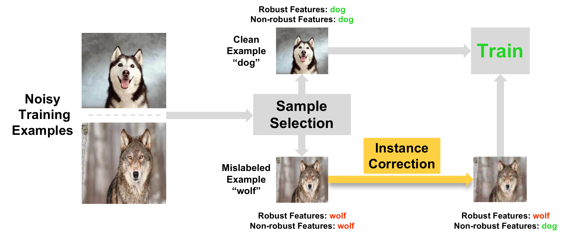
Figure 1: The illustration of the algorithm flow of the proposed method. When learning with open-set noisy labels, we first exploit the sample selection approach to distinguish the clean example “dog” and mislabeled example “wolf”. Then we employ targeted adversarial attacks to perform instance correction, which reserves robust features of the wolf and changes non-robust features of the wolf to those of the dog. Finally, we utilize both the clean example and corrected example for training with the supervision of the label “dog”.

In this paper, to relieve the issue of ignoring meaningful information of discarded data in learning with open-set noisy labels, we perform instance correction on discarded data to make use of them. Specifically, we employ targeted adversarial attacks [24] which attempt to change the output classification of the input to a special target class. For the discarded data, the adversarial targeted attacks make their instances match given labels actively. In this way, we can achieve instance correction to combat open-set noisy labels. The illustration of our method is provided in Figure 1.

The proposed instance correction is motivated by the fact that the features of an instance can be divided into robust features and non-robust features [12]. Compared with robust features which have been discussed, non-robust features are brittle and incomprehensible to we humans. Training with robust or non-robust features can yield great test accuracy [12]. Besides, non-robust features are easier to be changed with adversarial attacks than the robust ones [12]. For the instances with labels that are not contained within the known class label set in the training data, they may have some robust features like those in clean data to help generalization as discussed. However, they may have different non-robust features compared with clean ones, which do not help generalization. Therefore, we use targeted adversarial attacks to change such non-robust features to match given labels.

Before delving into details, we summarize the main contributions of this paper in two folds. First, we identify the issues of prior approaches on learning with open-set noisy labels and propose instance correction to relieve the issue of ignoring meaningful information in discarded data. Second, we conduct a series of experiments to justify our claims well. The rest of this paper is organized as follows. In Section 2, we introduce the background of learning with open-set noisy labels. In Section 3, we present how to make use of discarded data to enhance deep networks step by step. Experimental results are provided in Section 4. Finally, we conclude the paper in Section 5.

2 Learning with Open-set Noisy Labels

Notations. Vectors and matrices are denoted by bold-faced letters. We use $\|\cdot\|_{p}$ as the $\ell_{p}$ norm of vectors or matrices. Let $[z]=\{1,2,\ldots,z\}$.

Preliminaries. Consider a classification task, where there are $c$ classes in total. Let $\mathcal{X}$ and $\mathcal{Y}$ be the instance space and label space respectively, where $\mathcal{X}\in\mathbbm{R}^{d}$ with $d$ being the dimensionality, and $\mathcal{Y}=[c]$. In traditional supervised learning, the given training labels are clean. By employing such a clean dataset $S=\{(\mathbf{x}_{i},y_{i})\}_{i=1}^{n}$, where $n$ denotes the sample size or the number of training data, our goal is to learn a classifier that can assign labels precisely for given instances. However, in many real-world applications, the clean labels cannot be observed and the observed labels are noisy. Consider a subset of $S$ (denoted by $S^{\prime}$) is corrupted and denote the corrupted version of the subset $S^{\prime}$ by $S^{\star}$. Let $\mathcal{Y}^{\prime}$ be the label space of $S^{\star}$ (with $\mathcal{Y}^{\prime}\cap\mathcal{Y}=\varnothing$)—this means that the instances in $S^{\star}$ no longer have labels in $\mathcal{Y}$. Therefore, the whole noisy dataset can be denoted by $\tilde{S}=(S\backslash S^{\prime})\cup S^{\star}$. The aim is changed to learn a robust classifier that could assign clean labels to test data by exploiting the noisy dataset $\tilde{S}$.

Here, we provide an intuitive example for better understanding of the above notations (i.e., $S$, $S^{\prime}$, $S^{\star}$, and $\tilde{S}$) and problem setting, which is shown in Figure 2. We exploit the images of CIFAR-10 [15] and SVHN [27]. More specifically, the clean examples come from CIFAR-10, and the mislabeled examples (i.e., the examples in the set $S^{\star}$) come from SVHN. In the generation process of open-set noisy labels, part of images of CIFAR-10 are corrupted by the images of SVHN. Besides, the examples of CIFAR-10 and SVHN do not have the same label space. For this reason, we only have a noisy sample set, i.e. $\tilde{S}$, and need to learn a robust classifier that can assign labels to test data.

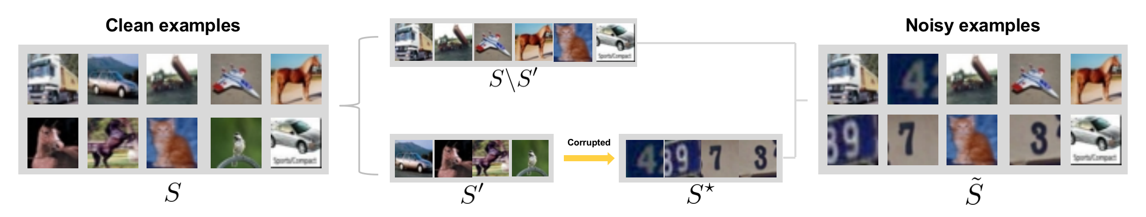
Figure 2: The illustration of the used notations and problem setting.

Limitations of loss/label correction approaches. The methods of loss correction and label correction cannot handle noisy labels well [37]. Here, we discuss the issues in more detail. For the loss correction approach, we need to model the flip processes from clean labels to noisy labels [43, 49, 18, 8, 32, 20], which are within the class label set of training data. When learning with open-set noisy labels, some instances do not have clean class labels which are within the class label set of training data. Therefore, when we tend to use the loss correction approach to handle open-set noisy labels, we will mistakenly assign labels to mislabeled data. If this happens, the correction of the training losses will be incorrect, following bad classification performance.

For the label correction approach [34, 55, 53], we need to recalibrate the labels of mislabeled data based on the predictions of classifiers. As the classifier is trained only with the known class label set, it assigns labels to mislabeled data from this set. Apparently, such an assignment is incorrect, since the true labels of the mislabeled data are outside the known class label set. As a result, we still train the classifier on the dataset which contains incorrect labels. Hence, the obtained classifier cannot be robust under this circumstance.

Shortcomings of the sample selection approach. Prior effects exploited sample selection to handle open-set noisy labels [37, 50], which only used the “clean” examples (with relatively small losses) from each mini-batch for training. Such approaches inherit the memorization effects of deep networks [1], which show that they would first memorize training data with clean labels and then those with noisy labels under the assumption that clean labels are of the majority in a noisy class. We use the self-teach model [13, 48] as a representative example. The procedure is shown in Algorithm 1. Let $f$ be the classifier with learnable parameters. At the $t$-th iteration, when a mini-batch $\bar{S}$ is formed (Step 5), a subset of small-loss examples $\bar{S}_{f}$ is selected from the mini-batch $\bar{S}$ (Step 6). The size of $\bar{S}_{f}$ is determined by $R(T)$, which always depends on the noise rate $\tau$ [9]. Note that in [9], the function $R(T)$ is designed as $1-\min\{{T}/{T_{k}}*\tau,\tau\}$. Such a design can help us make better use of the memorization effects of deep networks for sample selection. More specifically, deep networks will learn clean and easy pattern in the initial epochs [1]. Therefore, they have the ability to filter out mislabeled examples using their loss values at the beginning of training. When the number of epochs goes large, they will eventually overfit to noisy labels [9]. For this reason, at the start of training, we set $R(T)$ to a large value. Then, we gradually increase the drop rate, i.e., reduce the value of $R(T)$.

The selected “clean” examples are then used to update the network parameters in Step 7. Those “mislabeled” examples are discarded directly and do not participate in training. To the end, since we select less noisy data for parameters updates, the classifier $f$ will be more robust. Note that in Step 6, we select small-loss examples $\bar{S}_{f}$ from $\bar{S}$ for parameter updates, where the examples in $\bar{S}\backslash\bar{S}_{f}$ are seen to be useless and discarded from training. Nevertheless, as discussed, such data could consist of meaningful information for generalization. It thus is not a great choice to abandon them directly during training, which makes the sample selection approach achieve sub-optimal performance. We discuss how to address the issue using the proposed method in next section.

1:  Input: initialized classifier $f$, fixed $\tau$, epoch $T_{k}$ and $T_{\max}$, iteration $t_{\max}$.

2:  for $T=0,\dots,T_{\max}-1$ do

3:     Shuffle training set $\tilde{S}$;

4:     for $t=0,\dots,t_{\max}-1$ do

5:        Draw a mini-batch $\bar{S}$ from $\tilde{S}$;

6:        Select $R(T)$ small-loss examples $\bar{S}_{f}$ from $\bar{S}$ based on classifier’s predictions;

7:        Update classifier parameter only using $\bar{S}_{f}$;

8:     end for

9:     Update $R(T)=1-\min\{\frac{T}{T_{k}}\tau,\tau\}$;

10:  end for

11:  Output: trained classifier $f$.

Algorithm 1 General procedure on using sample selection to combat open-set noisy labels.

3 Method

In this section, we introduce the proposed method in more detail. Recall Algorithm 1, the set of discarded data in each mini-batch can be denoted by $\bar{S}\backslash\bar{S}_{f}$. We focus on how to make use of the training data in $\bar{S}\backslash\bar{S}_{f}$ to help generalization.

Recent work [12] showed that adversarial examples can be directly attributed to the presence of non-robust features, which are derived from patterns in the data distribution and highly predictive. Note that non-robustness does not mean that the model is brittle, but part of features of images are easy to be changed via adversarial attacks. Also, adversarial attacks mainly change the non-robust features [12]. Although non-robust features may be incomprehensible, they still can be used to achieve great classification performance. Therefore, for our method, it is reasonable to generalize well with corrected examples which are obtained by target adversarial attacks. We therefore can exploit targeted adversarial attacks on discarded data during training.

Let $\ell:\mathbbm{R}^{c}\times\mathcal{Y}\rightarrow\mathbbm{R}_{+}$ be a surrogate loss function for $c$-class classification. The loss function can be used to measure the degree of certainty that $f$ classifies the input to specific classes. In this paper, we exploit the softmax cross entropy loss. Given a discarded example $(\mathbf{x}_{i},\tilde{y}_{i})\in\bar{S}\backslash\bar{S}_{f}$, we construct an adversarial example from a benign example $\mathbf{x}_{i}$ by adding a perturbation vector $\delta_{\mathbf{x}_{i}}$ by solving the following optimization problem:

$$\min_{\delta_{\mathbf{x}_{i}}}\ell(f(\mathbf{x}_{i}+\delta_{\mathbf{x}_{i}}),\tilde{y}_{i})\ \text{subject to}\ \|\delta_{\mathbf{x}_{i}}\|_{2}\textless\rho\ \text{and}\ f(\mathbf{x}_{i}+\delta_{\mathbf{x}_{i}})=\tilde{y_{i}},$$ (1)

where $\rho$ is the budget of targeted adversarial attacks [2, 40, 21, 38]. When the classifier $f$ outputs probabilities $p_{f}(\cdot|\mathbf{x}_{i})$ associated with each class, the used adversarial loss is $\ell(f(\mathbf{x}_{i}+\delta_{\mathbf{x}_{i}}),\tilde{y}_{i})=-p_{f}(\tilde{y}_{i}|\mathbf{x}_{i}+\delta_{\mathbf{x}_{i}})$, which essentially maximizes the probability of classification into the class $\tilde{y}_{i}$. Here, we denote the corrected instance via targeted adversarial attacks by $\tilde{\mathbf{x}}_{i}$, i.e., $\tilde{\mathbf{x}}_{i}=\mathbf{x}_{i}+\delta_{\mathbf{x}_{i}}$. The set that includes the pairs of the corrected instances and given labels, i.e., $(\tilde{\mathbf{x}}_{j},\tilde{y}_{j})$, is denoted as $\bar{S}_{p}$.

In this way, although the clean label of the instance $\mathbf{x}_{i}$ is not within the class label set of the training data, the clean label of the corrected instance $\tilde{\mathbf{x}}_{i}$ can be seen as the given label $\tilde{y}_{i}$ from the perspective of classifier outputs. As such corrected instances can be highly predictive and help generalization, after targeted adversarial attacks, both the corrected examples and reserved examples in $\bar{S}_{f}$ are employed for network parameter updates. In this work, we seek a balance between corrected examples and reserved examples during training. Our objective function is given as follows:

$$\min L=\lambda*\ell_{(\mathbf{x}_{i},\tilde{y}_{i})\in\bar{S}_{f}}(f(\mathbf{x}_{i}),\tilde{y}_{i})+(1-\lambda)*\ell_{(\tilde{\mathbf{x}}_{j},\tilde{y}_{j})\in\bar{S}_{p}}(f(\tilde{\mathbf{x}}_{j}),\tilde{y}_{j}),$$ (2)

where $\lambda\geq 0$ is a hyperparameter to balance the contributions of corrected examples and reserved examples for training. More discussions about this hyperparameter are provided in Section 4.

Overall procedure. We summarize the overall procedure of the proposed method based on the self-teach model [13, 48]. Note that the proposed method can also be added to the methods which exploit two networks for sample selection, e.g., Co-teaching [9, 50]. We employ the self-teaching model as a representative example to be compared with Algorithm 1 more intuitively. We summarize the overall procedure of the proposed method in Algorithm 2. Specifically, we first use the sample selection approach to obtain an initialized classifier (Step 3). Then we divide all training examples into a clean set $\bar{S}_{f}$ and a mislabeled set $S\backslash\bar{S}_{f}$ (Step 5). After this, we perform instance correction on the instances in $S\backslash\bar{S}_{f}$ by using targeted adversarial attacks to make them match given labels and obtain the set $\bar{S}_{p}$ (Step 6). The new training example set which consists of both the corrected examples and selected examples is obtained for parameter updates (Step 8). Comparing Algorithm 1 with Algorithm 2 further, we can see that the proposed method are simply implemented based on the prior sample selection procedure. Note that the hyperparameter $T_{c}$ can be determined by using a noisy validation set. Although the noisy validation set cannot perform as good as the clean one, it does not introduce the assumption that some clean data are available, which is more realistic [28].

1:  Input: initialized classifier $f$, fixed $\tau$, epoch $T_{c}$ and $T_{\max}$.

2:  for $T=0,\dots,T_{c}-1$ do

3:     Use the sample selection approach as did in Algorithm 1;

14:  end for

5:  Divide all training examples into clean and mislabeled examples using predictions of $f$;

6:  Perform instance correction for the mislabeled examples;

7:  for $T=T_{c},\dots,T_{\max}-1$ do

8:     Exploit both clean and corrected examples for training as did in Eq. (2);

9:  end for

10:  Output: trained classifier $f$.

Algorithm 2 Overll procedure of the proposed method.

4 Experiments

In this section, we justify our claims from two folds. First, we conduct experiments on the benchmark dataset with synthetic open-set noisy labels (Section 4.1). Second, we conduct experiments on the real-world dataset which contains open-set noisy labels (Section 4.2).

4.1 Experiments on the benchmark dataset

Dataset. CIFAR-10 [15] is employed to verify the effectiveness of the proposed method, which is popularly used for evaluation of noisy labels in the literature [37, 42, 50, 35, 23, 22]. CIFAR-10 has 10 classes of color images including 50,000 training images and 10,000 test images. The size of color images is 32$\times$32.

Open-set noisy label generation. Following [37], open-set noisy datasets are built by replacing some training images in CIFAR-10 by outside images, while keeping the labels and the number of images per class unchanged. We consider two types of noise, i.e., Type I and Type II noise. Type I noise includes images from SVHN [27], CIFAR-100 [15], and ImageNet32 (32$\times$32 ImageNet images) [5], and only those images whose labels exclude the 10 classes in CIFAR-10 are considered. Type II noise includes images damaged by Gaussian random noise, corruption, resolution distortion, fog distortion, and motion blur distortion. Some examples of the type I and type II open-set noisy labels are given in Figure 3. The overall noise rate $\tau$ is set to 20%, 40%, 60%, and 80%. We leave out 10% of the noisy training data as a validation set for model selection.

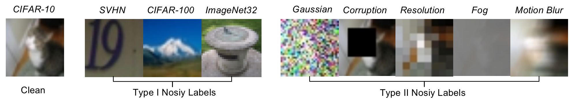
Figure 3: Illustrations of examples of the noise injected to CIFAR-10.

Baselines. We compare the proposed method with the state-of-the-arts and the most related techniques for learning with open-set noisy labels: (1) Forward [30], which estimates the noise transition matrix to combat noisy labels. (2) Joint [34], which jointly optimizes the labels of examples and the network parameters for label correction. (3) SIGUA [10], which exploits stochastic integrated gradient underweighted ascent to handle noisy labels. We use self-teach SIGUA in this paper. (4) MentorNet [13], which learns a curriculum to filter out noisy data. We used self-teach MentorNet in this paper. (5) S2E [48], which exploits the AutoML technology to handle noisy labels. Note that the baseline (1) belongs to the loss correction approach. The baselines (2) belong to the label correction approach. Besides, the baselines (3), (4), and (5) belong the sample selection approach.

Besides, we add a comparison called Mix, which directly involves discarded data into training without instance correction. Mix is based on the initialization of S2E. Our method, i.e., instance correction, is denoted as InsCorr in experiments. Since the proposed method is built on the sample selection approach, i.e., MentorNet (M) and S2E (S), we denote the proposed method as M-InsCorr and S-InsCorr respectively. Also, all methods Mix, M-InsCorr, and S-InsCorr are proposed in this paper, as prior works on sample selection do not make use of discarded data during training. We mark our methods with a symbol $\star$. Note that we do not compare our method with some state-of-the-art methods, e.g., SELF [28] and DivideMix [16]. It is because their proposed methods are aggregations of multiple techniques. The comparison with our method is thus not fair.

Experimental setup. For the fair comparison, we implement all methods with default parameters by PyTorch, and conduct all the experiments on NVIDIA Tesla V100 GPUs. A 7-layer CNN architecture is exploited following [37, 50], which is standard test bed for weakly-supervised learning. The network architecture consists of 6 convolutional layers and 1 fully-connected layer. Batch normalization is applied in each convolutional layer before the ReLU activation, and a max-pooling layer is implemented every two convolutional layers. For all experiments, Adam optimizer (momentum=0.9) is with an initial learning rate of 0.001, and the batch size is set to 128. We run 200 epochs in total. As for targeted adversarial attacks, we employ targeted LinfPGD-Attacks [24] with the budget 8/255 and borrow the implementation of the Advertorch toolbox [7].

For MentorNet and M-InsCorr, we set $R(T)=1-\min\{\frac{T}{T_{k}}\tau,\tau\}$. Here, we set $T_{k}$ to 10 as did in [50]. If the noise rate $\tau$ is not known in advanced, it can be inferred using validation sets [19, 51]. For S2E and S-InsCorr, we set $R(T)$ as did in [48], and exploit the official code . Note that $R(T)$ only depends on the memorization effect of deep networks but not any specific datasets [9]. As for the performance measurement, we use the test accuracy, i.e., test accuracy = (# of correct prediction) / (# of testing). All experiments on CIFAR-10 are repeated five times. We report the mean and standard deviation of experimental results. Intuitively, if a method can achieve higher classification performance, it can better handle open-set noisy labels.

Noise setting			Forward	Joint	SIGUA	Mix$\star$	MentorNet	M-InsCorr$\star$	S2E	S-InsCorr$\star$
C+S	20%	74.26 $\pm$0.49	79.11 $\pm$1.53	70.88 $\pm$2.33	80.68 $\pm$0.19	82.77 $\pm$0.30	82.81 $\pm$0.60	82.32 $\pm$0.80	82.58 $\pm$1.09
2-10[2pt/3pt]	40%	71.37 $\pm$0.52	74.71 $\pm$1.78	61.57 $\pm$2.00	75.71 $\pm$0.56	79.67 $\pm$0.21	80.03 $\pm$0.19	78.85 $\pm$1.86	79.16 $\pm$1.35
2-10[2pt/3pt]	60%	53.83 $\pm$2.37	68.09 $\pm$1.31	54.71 $\pm$2.04	60.47 $\pm$0.44	72.68 $\pm$3.95	72.05 $\pm$0.62	73.82 $\pm$2.69	73.72 $\pm$1.19
2-10[2pt/3pt]	80%	36.25 $\pm$0.84	39.06 $\pm$3.12	20.77 $\pm$2.16	59.61 $\pm$0.64	64.90 $\pm$2.19	62.35 $\pm$0.32	63.03 $\pm$1.11	62.36 $\pm$1.55
C+C	20%	76.72 $\pm$0.93	75.37 $\pm$1.47	74.27 $\pm$0.16	77.79 $\pm$0.27	82.14 $\pm$0.15	81.64 $\pm$0.52	80.34 $\pm$0.79	80.02 $\pm$0.90
2-10[2pt/3pt]	40%	72.07 $\pm$1.39	67.30 $\pm$0.39	68.08 $\pm$0.29	68.79 $\pm$0.26	79.17 $\pm$0.15	79.65 $\pm$1.03	73.47 $\pm$5.60	74.52 $\pm$2.73
2-10[2pt/3pt]	60%	54.95 $\pm$1.06	52.58 $\pm$4.62	53.45 $\pm$1.46	58.89 $\pm$0.07	74.58 $\pm$0.31	74.86 $\pm$0.28	60.77 $\pm$7.46	62.09 $\pm$3.43
2-10[2pt/3pt]	80%	32.93 $\pm$2.44	42.95 $\pm$1.29	26.66 $\pm$4.37	40.41 $\pm$0.89	57.53 $\pm$0.23	57.73 $\pm$0.93	42.73 $\pm$7.61	46.24 $\pm$2.65
C+I	20%	77.12 $\pm$0.38	76.79 $\pm$1.36	72.16 $\pm$0.92	80.66 $\pm$0.21	82.15 $\pm$0.77	82.47 $\pm$0.06	80.25 $\pm$1.02	80.74 $\pm$0.91
2-10[2pt/3pt]	40%	70.74 $\pm$1.17	65.76 $\pm$2.64	70.93 $\pm$1.40	73.47 $\pm$1.01	78.60 $\pm$0.46	79.05 $\pm$0.15	77.33 $\pm$2.72	77.87 $\pm$2.24
2-10[2pt/3pt]	60%	60.30 $\pm$2.56	57.62 $\pm$1.50	59.54 $\pm$1.65	60.63 $\pm$0.47	73.06 $\pm$2.31	71.33 $\pm$0.62	64.09 $\pm$2.88	64.01 $\pm$2.60
2-10[2pt/3pt]	80%	35.60 $\pm$1.49	37.09 $\pm$4.06	20.58 $\pm$0.96	40.09 $\pm$3.61	58.06 $\pm$3.76	56.24 $\pm$2.24	46.95 $\pm$2.62	49.62 $\pm$3.04

Table 1: Mean and standard deviation of test accuracy (%) of different methods for learning with Type I open-set noisy labels over last ten epochs. “C+S” is the abbreviation of CIFAR-10+SVHN. “C+C” is the abbreviation of CIFAR-10+CIFAR-100. “C+S” is the abbreviation of CIFAR-10+ImageNet32. The methods with the mark $\star$ are our methods. The best results are in bold.

Noise setting			Forward	Joint	SIGUA	Mix$\star$	MentorNet	M-InsCorr$\star$	S2E	S-InsCorr$\star$
C+G	20%	74.62 $\pm$0.88	79.00 $\pm$0.84	75.97 $\pm$0.21	80.33 $\pm$0.65	80.56 $\pm$0.20	81.17 $\pm$0.43	79.53 $\pm$2.14	79.80 $\pm$1.35
2-10[2pt/3pt]	40%	71.45 $\pm$1.17	75.11 $\pm$0.12	60.88 $\pm$0.15	75.15 $\pm$0.35	73.35 $\pm$0.38	76.32 $\pm$0.27	76.06 $\pm$1.52	76.33 $\pm$0.32
2-10[2pt/3pt]	60%	60.62 $\pm$1.86	70.30 $\pm$0.42	37.69 $\pm$5.62	59.84 $\pm$1.10	56.93 $\pm$0.68	64.64 $\pm$0.71	71.80 $\pm$1.46	72.25 $\pm$1.83
2-10[2pt/3pt]	80%	33.06 $\pm$1.78	53.17 $\pm$3.94	35.66 $\pm$1.92	53.98 $\pm$1.77	27.86 $\pm$1.30	48.44 $\pm$3.05	62.74 $\pm$2.83	63.50 $\pm$2.11
C+O	20%	75.79 $\pm$1.05	78.93 $\pm$1.36	66.33 $\pm$0.31	82.41 $\pm$0.49	81.81 $\pm$0.31	82.55 $\pm$0.35	79.47 $\pm$2.96	79.65 $\pm$2.36
2-10[2pt/3pt]	40%	75.44 $\pm$0.93	75.82 $\pm$1.25	60.08 $\pm$0.83	80.17 $\pm$0.02	75.16 $\pm$0.37	77.51 $\pm$0.09	79.21 $\pm$2.41	79.44 $\pm$2.63
2-10[2pt/3pt]	60%	64.05 $\pm$0.87	74.36 $\pm$0.63	30.08 $\pm$1.00	77.84 $\pm$0.27	57.09 $\pm$0.60	72.00 $\pm$0.68	77.73 $\pm$1.80	77.90 $\pm$1.08
2-10[2pt/3pt]	80%	47.92 $\pm$2.37	67.32 $\pm$0.88	28.75 $\pm$1.06	69.54 $\pm$0.25	29.75 $\pm$1.64	64.75 $\pm$0.91	70.26 $\pm$1.34	71.05 $\pm$0.30
C+R	20%	77.46 $\pm$0.94	82.22 $\pm$0.50	66.19 $\pm$0.22	82.48 $\pm$0.49	82.58 $\pm$0.12	82.91 $\pm$0.13	79.18 $\pm$1.41	79.77 $\pm$0.69
2-10[2pt/3pt]	40%	74.09 $\pm$1.88	78.80 $\pm$1.56	57.88 $\pm$0.58	79.00 $\pm$0.16	74.43 $\pm$0.25	79.07 $\pm$0.12	78.75 $\pm$2.65	79.07 $\pm$2.39
2-10[2pt/3pt]	60%	65.63 $\pm$1.05	75.39 $\pm$2.31	28.84 $\pm$1.86	76.04 $\pm$0.60	56.91 $\pm$0.84	72.51 $\pm$0.79	76.65 $\pm$2.24	77.25 $\pm$2.21
2-10[2pt/3pt]	80%	41.65 $\pm$3.93	52.65 $\pm$1.79	20.06 $\pm$3.43	65.19 $\pm$1.87	29.62 $\pm$0.77	62.91 $\pm$1.15	70.73 $\pm$2.84	71.31 $\pm$2.12
C+F	20%	75.45 $\pm$0.93	81.18 $\pm$0.44	70.09 $\pm$0.43	83.48 $\pm$0.24	82.70 $\pm$0.23	82.81 $\pm$0.92	83.15 $\pm$1.34	83.52 $\pm$1.37
2-10[2pt/3pt]	40%	75.10 $\pm$1.52	78.91 $\pm$0.56	62.39 $\pm$0.70	81.05 $\pm$0.24	81.84 $\pm$0.54	82.03 $\pm$0.09	82.83 $\pm$0.23	82.87 $\pm$0.35
2-10[2pt/3pt]	60%	66.08 $\pm$0.83	73.37 $\pm$0.82	40.24 $\pm$0.95	78.18 $\pm$0.14	76.72 $\pm$0.32	77.23 $\pm$0.52	78.76 $\pm$0.17	79.03 $\pm$1.09
2-10[2pt/3pt]	80%	53.22 $\pm$1.17	68.06 $\pm$1.78	38.62 $\pm$0.73	69.89 $\pm$0.73	60.25 $\pm$0.31	61.02 $\pm$0.39	70.55 $\pm$0.54	71.19 $\pm$0.67
C+M	20%	77.79 $\pm$0.75	81.36 $\pm$0.32	68.50 $\pm$0.23	81.45 $\pm$0.21	82.61 $\pm$0.42	82.66 $\pm$0.14	79.98 $\pm$1.32	80.16 $\pm$1.11
2-10[2pt/3pt]	40%	75.13 $\pm$0.68	78.24 $\pm$1.05	61.05 $\pm$0.90	78.56 $\pm$0.19	74.71 $\pm$0.41	77.30 $\pm$0.92	78.58 $\pm$2.09	79.30 $\pm$1.77
2-10[2pt/3pt]	60%	64.75 $\pm$1.62	75.36 $\pm$0.61	33.44 $\pm$2.60	75.13 $\pm$0.24	57.34 $\pm$2.38	70.06 $\pm$0.49	76.34 $\pm$1.85	76.49 $\pm$2.68
2-10[2pt/3pt]	80%	60.40 $\pm$1.08	64.39 $\pm$2.82	28.77 $\pm$1.06	68.58 $\pm$0.64	28.65 $\pm$1.62	61.72 $\pm$0.66	69.36 $\pm$1.25	71.02 $\pm$0.63

Table 2: Mean and standard deviation of test accuracy (%) of different methods for learning with Type II open-set noisy labels over last ten epochs. “C+G” is the abbreviation of CIFAR-10+Gaussian. “C+O” is the abbreviation of CIFAR-10+Corruption. “C+R” is the abbreviation of CIFAR-10+Resolution. “C+F” is the abbreviation of CIFAR-10+Fog. “C+M” is the abbreviation of CIFAR-10+Motion Blur. The methods with the mark $\star$ are our methods. The best results are in bold.

4.1.1 Analyses of experimental results

Overall results. The experimental results with Type I and Type II open-set noise are provided in Table 1 and 2 respectively. With Type I open-set noise, the sample selection approach (e.g., MentorNet) always outperforms other types of approaches. When the noise level is high, the advantage is very obvious. For example, when the noise rate is 80%, MentorNet always achieves a lead of more than 10% over Joint. In addition, MentorNet achieves a lead of more than 20% over Forward. The experimental results show the superiority of the sample selection approach in combating open-set noisy labels.

With Type II open-set noise, the sample selection approach S2E achieves the best classification performance in most cases. When the noise level is high, the performance of another sample selection approach MentorNet is not promising. The reason is that MentorNet exploits a fixed sample selection procedure, i.e., $R(T)$. Also, when the noise level is high, it easily chooses the mislabeled examples, since the mislabeled ones are more similar with original ones in Type II open-set noise. What’s worse, once MentorNet makes the wrong choice during training, the errors will be accumulated, which seriously hurts generalization [50]. By contrast, S2E exploits the AutoML technique to control the sample selection procedure, which better exploits the memorization effects of deep networks, following better classification performance than MentorNet. Although SIGUA also focuses on sample selection, it uses stochastic integrated gradient underweighted ascent to handle open-set noisy labels, which highly relies on suitable selection of hyperparameters. Therefore, SIGUA does not achieve competitive performance with other sample selection methods.

Mix vs. loss/label correction. As shown in Table 1, on C+S and C+C, Mix can outperform Forward and Joint in most cases. On C+I, Mix always achieves better classification performance than Forward and Joint. Such experimental results show the vulnerability of the loss and label correction approaches to handle open-set noisy labels. Similarly, as shown in Table 2, Mix can obtain better results compared with Forward and Joint in most circumstances.

InsCorr vs. sample selection. We first analyze the results with Type I open-set noise. In the most cases, the proposed instance correction can bring positive effects for generalization, which show the effectiveness of the proposed method. In some cases, instance correction cannot bring better performance. The reason is that Type I open-set noise is generated too randomly or even groundlessly. Therefore, the mislabeled examples consist of too many distinct robust features, which make it difficult to correct them by the proposed method. For instance, the images of CIFAR-10 is mainly about the objects in our daily life, e.g., cats, dogs, and frogs. However, the images of SVHN is about the house numbers in Google Street View imagery. The images in two datasets are much different, which causes that instance correction sometimes does not work well.

We then analyze the results with Type II open-set noise, where the noise is arguably generated more reasonably. In such cases, instance correction can change the non-robust features of mislabeled examples to match given labels, which brings better classification performance. The results justify our claims well, i.e., the discard data may have meaningful information, and can be used for training.

4.1.2 Ablation study

We conduct an ablation study to analyze the influence of the hyperparameter $\lambda$ and show the impact of the discarded data. The experiments are conducted on the Type I noise datasets (i.e., C+S, C+C, and C+I) and the Type II noise datasets (i.e., C+O, C+R, and C+F). The experimental settings such as the network architecture and optimizer have been introduced before. The value of $\lambda$ is chosen from the range $\{0.05,0.10,0.15,0.20,0.25,0.30\}$. The illustrations of results are provided in Figure 4.

The discarded data have different influences in the experiments with Type I and Type II open-set noise. More specifically, with Type I open-set noise, we can see that the test accuracy decreases if we increase the the value of $\lambda$ in almost every case. Such results mean that the mislabeled examples in Type I cannot be directly involved into training, since they would hurt generalization. We need to first correct them and then can utilize them. As a comparison, with Type II open-set noise, the curve of test accuracy is not monotonically decreasing with the increase of $\lambda$. The results mean that the discarded data have positive effects to help generalization. Hence, we can make use of them appropriately. Note that such differences of results lie in the differences between the two noise generation mechanisms, which also show that the direct use of discarded data may be invalid.

C+S

C+C

C+I

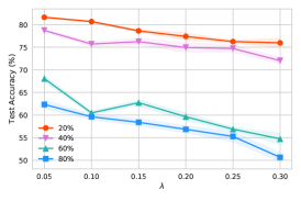
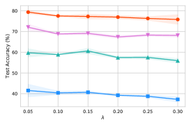
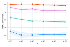
– Type I –

C+O

C+R

C+F

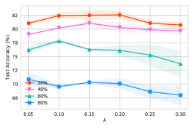
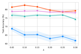
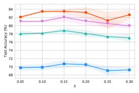
– Type II –

Figure 4: Illustrations of the test accuracy of the method Mix with different $\lambda$. The error bar for standard deviation in each figure has been shaded.

4.2 Experiments on the real-world dataset

Experimental setup. The WebVision [17] dataset is employ in this paper. WebVision contains 2.4 million images crawled from the websites using the 1,000 concepts in ImageNet ILSVRC12 [6]. Following the “Mini” setting in [13, 3, 23], we take the first 50 classes of the Google resized image subset, and evaluate the trained networks on the same 50 classes of the ILSVRC12 validation set, which is exploited as a test set. Following prior works [30, 42], we leave out 10% training data as a validation set, which is for model selection. For WebVision, we use an Inception-ResNet v2 [33] with batch size 128. The initial learning rate is set to $10^{-1}$. We set 100 epochs in total for all the experiments on the real-world dataset.

Forward	Joint	SIGUA	Mix$\star$	MentorNet	M-InsCorr$\star$	S2E	S-InsCorr$\star$
56.39	47.60	40.35	54.39	57.66	57.89	57.05	57.75

Table 3: Top-1 validation accuracies (%) on clean ILSVRC12 validation set of Inception-ResNet v2 models trained on WebVision, under the “Mini” setting in [13, 3, 23]. The best result is in bold.

Experimental results. The experimental results are provided in Table 3. Comparing M-InsCorr with MentorNet, we achieve an improvement of +0.23%. Besides, comparing S-InsCorr with S2E, we achieve an improvement of +0.70%. Note that directly involving discarded data can outperform the baselines such as Joint clearly, which means this type of approach is somewhat vulnerable in the practical problem. The results on the real-world dataset mean that the proposed method can handle classification tasks well in actual scenarios.

5 Conclusion

In this paper, we focus on the problem of learning with open-set noisy labels, where part of training data have a different label space that does not contain the true class. We first point out the weaknesses of the approaches such as loss correction, label correction, and sample selection for handling open-set noisy labels. Then we propose to use instance correction which is performed by targeted adversarial attacks to corrected the instances of discarded data to utilize them for training. A series of experimental results justify our claims well and verify the effectiveness of the proposed method. We believe that this paper opens up new possibilities in the topic of learning with open-set noisy labels. In the future, we will explore more ways to make use of discarded data and investigate more manners to perform instance correction to improve the robustness against open-set noisy labels.

References

- Arpit et al. [2017] Devansh Arpit, Stanisław Jastrzębski, Nicolas Ballas, David Krueger, Emmanuel Bengio, Maxinder S Kanwal, Tegan Maharaj, Asja Fischer, Aaron Courville, Yoshua Bengio, et al. A closer look at memorization in deep networks. arXiv preprint arXiv:1706.05394, 2017.
- Bai et al. [2021] Yang Bai, Yuyuan Zeng, Yong Jiang, Shu-Tao Xia, Xingjun Ma, and Yisen Wang. Improving adversarial robustness via channel-wise activation suppressing. arXiv preprint arXiv:2103.08307, 2021.
- Chen et al. [2019] Pengfei Chen, Ben Ben Liao, Guangyong Chen, and Shengyu Zhang. Understanding and utilizing deep neural networks trained with noisy labels. In ICML, pages 1062–1070, 2019.
- Cheng et al. [2020] Jiacheng Cheng, Tongliang Liu, Kotagiri Ramamohanarao, and Dacheng Tao. Learning with bounded instance-and label-dependent label noise. In ICML, 2020.
- Chrabaszcz et al. [2017] Patryk Chrabaszcz, Ilya Loshchilov, and Frank Hutter. A downsampled variant of imagenet as an alternative to the cifar datasets. arXiv preprint arXiv:1707.08819, 2017.
- Deng et al. [2009] Jia Deng, Wei Dong, Richard Socher, Li-Jia Li, Kai Li, and Li Fei-Fei. Imagenet: A large-scale hierarchical image database. In CVPR, pages 248–255. Ieee, 2009.
- Ding et al. [2019] Gavin Weiguang Ding, Luyu Wang, and Xiaomeng Jin. AdverTorch v0.1: An adversarial robustness toolbox based on pytorch. arXiv preprint arXiv:1902.07623, 2019.
- Han et al. [2018a] Bo Han, Jiangchao Yao, Gang Niu, Mingyuan Zhou, Ivor Tsang, Ya Zhang, and Masashi Sugiyama. Masking: A new perspective of noisy supervision. In NeurIPS, pages 5836–5846, 2018a.
- Han et al. [2018b] Bo Han, Quanming Yao, Xingrui Yu, Gang Niu, Miao Xu, Weihua Hu, Ivor Tsang, and Masashi Sugiyama. Co-teaching: Robust training of deep neural networks with extremely noisy labels. In NeurIPS, pages 8527–8537, 2018b.
- Han et al. [2020] Bo Han, Gang Niu, Xingrui Yu, Quanming Yao, Miao Xu, Ivor W Tsang, and Masashi Sugiyama. Sigua: Forgetting may make learning with noisy labels more robust. In ICML, 2020.
- Hendrycks et al. [2018] Dan Hendrycks, Mantas Mazeika, Duncan Wilson, and Kevin Gimpel. Using trusted data to train deep networks on labels corrupted by severe noise. In NeurIPS, pages 10456–10465. 2018.
- Ilyas et al. [2019] Andrew Ilyas, Shibani Santurkar, Dimitris Tsipras, Logan Engstrom, Brandon Tran, and Aleksander Madry. Adversarial examples are not bugs, they are features. arXiv preprint arXiv:1905.02175, 2019.
- Jiang et al. [2018] Lu Jiang, Zhengyuan Zhou, Thomas Leung, Li-Jia Li, and Li Fei-Fei. MentorNet: Learning data-driven curriculum for very deep neural networks on corrupted labels. In ICML, pages 2309–2318, 2018.
- Jiang et al. [2020] Lu Jiang, Di Huang, Mason Liu, and Weilong Yang. Beyond synthetic noise: Deep learning on controlled noisy labels. In ICML, pages 4804–4815, 2020.
- Krizhevsky and Hinton [2009] Alex Krizhevsky and Geoffrey Hinton. Learning multiple layers of features from tiny images. Technical report, 2009.
- Li et al. [2020] Junnan Li, Richard Socher, and Steven C.H. Hoi. Dividemix: Learning with noisy labels as semi-supervised learning. In ICLR, 2020.
- Li et al. [2017] Wen Li, Limin Wang, Li Wei, Eirikur Agustsson, and Luc Van Gool. Webvision database: Visual learning and understanding from web data. arXiv preprint arXiv:1708.02862, 2017.
- Li et al. [2021] Xuefeng Li, Tongliang Liu, Bo Han, Gang Niu, and Masashi Sugiyama. Provably end-to-end label-noise learning without anchor points. In ICML, 2021.
- Liu and Tao [2016] Tongliang Liu and Dacheng Tao. Classification with noisy labels by importance reweighting. IEEE Transactions on Pattern Analysis and Machine Intelligence, 38(3):447–461, 2016.
- Liu and Guo [2020] Yang Liu and Hongyi Guo. Peer loss functions: Learning from noisy labels without knowing noise rates. In ICML, 2020.
- Ma et al. [2018a] Xingjun Ma, Bo Li, Yisen Wang, Sarah M Erfani, Sudanthi Wijewickrema, Grant Schoenebeck, Dawn Song, Michael E Houle, and James Bailey. Characterizing adversarial subspaces using local intrinsic dimensionality. arXiv preprint arXiv:1801.02613, 2018a.
- Ma et al. [2018b] Xingjun Ma, Yisen Wang, Michael E Houle, Shuo Zhou, Sarah M Erfani, Shu-Tao Xia, Sudanthi Wijewickrema, and James Bailey. Dimensionality-driven learning with noisy labels. In ICML, pages 3361–3370, 2018b.
- Ma et al. [2020] Xingjun Ma, Hanxun Huang, Yisen Wang, Simone Romano, Sarah Erfani, and James Bailey. Normalized loss functions for deep learning with noisy labels. In ICML, 2020.
- Madry et al. [2018] Aleksander Madry, Aleksandar Makelov, Ludwig Schmidt, Dimitris Tsipras, and Adrian Vladu. Towards deep learning models resistant to adversarial attacks. In ICLR, 2018.
- Malach and Shalev-Shwartz [2017] Eran Malach and Shai Shalev-Shwartz. Decoupling" when to update" from" how to update". In NeurIPS, pages 960–970, 2017.
- Menon et al. [2020] Aditya Krishna Menon, Ankit Singh Rawat, Sashank J Reddi, and Sanjiv Kumar. Can gradient clipping mitigate label noise? In ICLR, 2020.
- Netzer et al. [2011] Yuval Netzer, Tao Wang, Adam Coates, Alessandro Bissacco, Bo Wu, and Andrew Y.Ng. Reading digits in natural images with unsupervised feature learning. In NIPS Workshop on Deep Learning and Unsupervised Feature Learning, 2011.
- Nguyen et al. [2020] Duc Tam Nguyen, Chaithanya Kumar Mummadi, Thi Phuong Nhung Ngo, Thi Hoai Phuong Nguyen, Laura Beggel, and Thomas Brox. Self: Learning to filter noisy labels with self-ensembling. In ICLR, 2020.
- Northcutt et al. [2021] Curtis G Northcutt, Lu Jiang, and Isaac L Chuang. Confident learning: Estimating uncertainty in dataset labels. Journal of Artificial Intelligence Research, 2021.
- Patrini et al. [2017] Giorgio Patrini, Alessandro Rozza, Aditya Krishna Menon, Richard Nock, and Lizhen Qu. Making deep neural networks robust to label noise: A loss correction approach. In CVPR, pages 1944–1952, 2017.
- Pleiss et al. [2020] Geoff Pleiss, Tianyi Zhang, Ethan R Elenberg, and Kilian Q Weinberger. Identifying mislabeled data using the area under the margin ranking. arXiv preprint arXiv:2001.10528, 2020.
- Shu et al. [2020] Jun Shu, Qian Zhao, Zengben Xu, and Deyu Meng. Meta transition adaptation for robust deep learning with noisy labels. arXiv preprint arXiv:2006.05697, 2020.
- Szegedy et al. [2016] Christian Szegedy, Sergey Ioffe, Vincent Vanhoucke, and Alex Alemi. Inception-v4, inception-resnet and the impact of residual connections on learning. arXiv preprint arXiv:1602.07261, 2016.
- Tanaka et al. [2018] Daiki Tanaka, Daiki Ikami, Toshihiko Yamasaki, and Kiyoharu Aizawa. Joint optimization framework for learning with noisy labels. In CVPR, 2018.
- Thulasidasan et al. [2019] Sunil Thulasidasan, Tanmoy Bhattacharya, Jeff Bilmes, Gopinath Chennupati, and Jamal Mohd-Yusof. Combating label noise in deep learning using abstention. In ICML, pages 6234–6243, 2019.
- Wang et al. [2019a] Xiaobo Wang, Shuo Wang, Jun Wang, Hailin Shi, and Tao Mei. Co-mining: Deep face recognition with noisy labels. In ICCV, pages 9358–9367, 2019a.
- Wang et al. [2018] Yisen Wang, Weiyang Liu, Xingjun Ma, James Bailey, Hongyuan Zha, Le Song, and Shu-Tao Xia. Iterative learning with open-set noisy labels. In CVPR, pages 8688–8696, 2018.
- Wang et al. [2019b] Yisen Wang, Xingjun Ma, James Bailey, Jinfeng Yi, Bowen Zhou, and Quanquan Gu. On the convergence and robustness of adversarial training. In ICML, volume 1, page 2, 2019b.
- Wang et al. [2019c] Yisen Wang, Xingjun Ma, Zaiyi Chen, Yuan Luo, Jinfeng Yi, and James Bailey. Symmetric cross entropy for robust learning with noisy labels. In ICCV, pages 322–330, 2019c.
- Wu et al. [2020] Dongxian Wu, Shu-Tao Xia, and Yisen Wang. Adversarial weight perturbation helps robust generalization. NeurIPS, 2020.
- Wu et al. [2021] Songhua Wu, Xiaobo Xia, Tongliang Liu, Bo Han, Mingming Gong, Nannan Wang, Haifeng Liu, and Gang Niu. Class2simi: A noise reduction perspective on learning with noisy labels. In ICML, 2021.
- [42] Xiaobo Xia, Tongliang Liu, Bo Han, Chen Gong, Nannan Wang, Zongyuan Ge, and Yi Chang. Robust early-learning: Hindering the memorization of noisy labels. In ICLR.
- Xia et al. [2019] Xiaobo Xia, Tongliang Liu, Nannan Wang, Bo Han, Chen Gong, Gang Niu, and Masashi Sugiyama. Are anchor points really indispensable in label-noise learning? In NeurIPS, pages 6838–6849, 2019.
- Xia et al. [2020] Xiaobo Xia, Tongliang Liu, Bo Han, Nannan Wang, Mingming Gong, Haifeng Liu, Gang Niu, Dacheng Tao, and Masashi Sugiyama. Part-dependent label noise: Towards instance-dependent label noise. In NeurIPS, 2020.
- Xiao et al. [2015] Tong Xiao, Tian Xia, Yi Yang, Chang Huang, and Xiaogang Wang. Learning from massive noisy labeled data for image classification. In CVPR, pages 2691–2699, 2015.
- Yan et al. [2014] Yan Yan, Rómer Rosales, Glenn Fung, Ramanathan Subramanian, and Jennifer Dy. Learning from multiple annotators with varying expertise. Machine learning, 95(3):291–327, 2014.
- Yang et al. [2021] Shuo Yang, Lu Liu, and Min Xu. Free lunch for few-shot learning: Distribution calibration. In ICLR, 2021.
- Yao et al. [2020a] Quanming Yao, Hansi Yang, Bo Han, Gang Niu, and James T Kwok. Searching to exploit memorization effect in learning with noisy labels. In ICML, 2020a.
- Yao et al. [2020b] Yu Yao, Tongliang Liu, Bo Han, Mingming Gong, Jiankang Deng, Gang Niu, and Masashi Sugiyama. Dual t: Reducing estimation error for transition matrix in label-noise learning. In NeurIPS, 2020b.
- Yu et al. [2019] Xingrui Yu, Bo Han, Jiangchao Yao, Gang Niu, Ivor W Tsang, and Masashi Sugiyama. How does disagreement benefit co-teaching? In ICML, 2019.
- Yu et al. [2018a] Xiyu Yu, Tongliang Liu, Mingming Gong, Kayhan Batmanghelich, and Dacheng Tao. An efficient and provable approach for mixture proportion estimation using linear independence assumption. In CVPR, pages 4480–4489, 2018a.
- Yu et al. [2018b] Xiyu Yu, Tongliang Liu, Mingming Gong, and Dacheng Tao. Learning with biased complementary labels. In ECCV, pages 68–83, 2018b.
- Zhang et al. [2021] Yikai Zhang, Songzhu Zheng, Pengxiang Wu, Mayank Goswami, and Chao Chen. Learning with feature-dependent label noise: A progressive approach. In ICLR, 2021.
- Zhang and Sabuncu [2018] Zhilu Zhang and Mert Sabuncu. Generalized cross entropy loss for training deep neural networks with noisy labels. In NeurIPS, pages 8778–8788, 2018.
- Zheng et al. [2020] Songzhu Zheng, Pengxiang Wu, Aman Goswami, Mayank Goswami, Dimitris Metaxas, and Chao Chen. Error-bounded correction of noisy labels. In ICML, 2020.