Wave-packet continuum discretisation for nucleon-nucleon scattering predictions

Abstract

In this paper we analyse the efficiency, precision, and accuracy of computing elastic nucleon-nucleon (NN) scattering amplitudes with the wave-packet continuum discretisation method (WPCD). This method provides approximate scattering solutions at multiple scattering energies simultaneously. We therefore utilise a graphics processing unit (GPU) to explore the benefits of this inherent parallelism. From a theoretical perspective, the WPCD method promises a speedup compared to a standard matrix-inversion method. We use the chiral NNLO_opt interaction to demonstrate that WPCD enables efficient computation of NN scattering amplitudes provided one can tolerate an averaged method error of $~{}1-5$ mb in the total cross section at scattering energies $0-350$ MeV in the laboratory frame of reference. Considering only scattering energies $\sim 40-350$ MeV, we find a smaller method error of $\lesssim 1-2$ mb. By increasing the number of wave-packets we can further reduce the overall method error. However, the parallel leverage of the WPCD method will be offset by the increased size of the resulting discretisation mesh. In practice, a GPU-implementation is mainly advantageous for matrices that fit in the fast on-chip shared memory. We find that WPCD is a promising method for computationally efficient, statistical analyses of nuclear interactions from effective field theory, where we can utilise Bayesian inference methods to incorporate relevant uncertainties.

Keywords: nucleon-nucleon scattering, wave-packet continuum discretization, chiral effective field theory

1 Introduction

A large portion of interaction-potential models currently applied in ab initio many-nucleon calculations are constructed using ideas from chiral effective field theory ($\chi$EFT) [1, 2, 3, 4]. Such potentials typically contain $\gtrsim$10-30 low-energy constants (LECs), acting as physical calibration parameters, that must be inferred from data. Bayesian methods for parameter estimation offer several advantages in this regard, in particular in conjunction with EFTs, see e.g. Ref. [5]. However, making reliable inferences typically incur a high total computational cost due to the large amount of posterior samples. It is therefore important to establish an efficient computational framework for generating model predictions of physical observables.

In this paper we look to low-energy nucleon-nucleon (NN) scattering cross sections as it constitutes the bulk part of the standard dataset for inferring the most probable values of the LECs, see e.g. Refs. [6, 7, 8, 9]. The most recent, and statistically consistent, database [10] of NN scattering cross sections contains data for thousands of measured proton-proton (pp) and neutron-proton (np) cross sections at hundreds of different laboratory scattering energies, mostly below the pion-production threshold at $T_{\text{lab}}\approx 290$ MeV. In most cases, the computational bottleneck when predicting NN scattering amplitudes for a given interaction potential comes from obtaining numerical solutions to the Lippmann-Schwinger (LS) equation.

There are essentially three approaches for improving computational efficiency and speed of a computational procedure: i) develop improved numerical methods and algorithms tailored to the physical model at hand and its application, ii) use specific hardware, e.g. a faster CPU, increased memory bandwidth, or parallel architectures such as in a graphics processing unit (GPU) to better handle some of the most dominant computational procedures of the model, or iii) replace any computationally expensive model evaluations with a fast, as well as sufficiently accurate and precise, surrogate model, i.e. an emulator, which mimics the original model output. This latter approach is very interesting and in particular eigenvector continuation (EC) [11, 12] applied to emulate NN-scattering amplitudes [13, 14] shows great promise, although uncertainty quantification is yet to be explored. Note, however, that EC emulation attains most of its speedup when applied to potential models that exhibit linear parameter dependencies. In cases where such dependencies are not present one might resort to other methods to handle the non-linear response, such as EC combined with Gaussian process emulation  [15]. However, one should note that Gaussian process emulation [16] and other standard machine learning methods exhibit poor scaling with increasing dimensionality of the input parameter domain.

Here, we will focus on approaches i) and ii) by exploring both the standard matrix-inversion (MI) method, see e.g. Ref. [17], and the wave-packet continuum discretisation (WPCD) method [18] for solving the LS equation. The WPCD method basically corresponds to a bound-state approach that uses eigenfunctions of the full NN Hamiltonian to approximate scattering solutions at any on-shell energy. This method is particularly interesting since it provides approximate scattering amplitudes at multiple scattering energies simultaneously. We have therefore implemented this inherently parallel method on a GPU. We also note that WPCD places no constraint on the analytical form of the potential or its parametric dependence. As such, WPCD acceleration for NN scattering complements the EC approaches for emulation [13, 14, 15] mentioned above.

Speeding up computations very often comes at the expense of accuracy and/or precision, and the WPCD method is no exception to this principle. The magnitude of experimental errors in the calibration data and the estimated theoretical model-discrepancies [19] provide natural tolerances for the level of method error that is acceptable. Indeed it is undesirable to have a method error that dominates the error budget such that it obscures or even hampers the inference of useful information. We therefore analyse the WPCD method in detail and quantify realistic computational speedups and compare the method errors to recent estimates of the model discrepancy in $\chi$EFT [20]. We also analyse and compare the numerical complexities of the MI and WPCD methods.

2 Nucleon-Nucleon Scattering

The LS equation, in operator form, for the transition-matrix operator $\hat{T}$ at some scattering energy $E$ is given by

$$\hat{T}(E)=\hat{v}+\hat{v}\hat{g}_{0}(E)\hat{T}.$$ (1)

This is an inhomogeneous Fredholm integral equation where $\hat{v}$ is some NN-potential operator, $\hat{g}_{0}(E)=(E-\hat{h}_{0}+i\epsilon)^{-1}$ is the free Green’s function, and $\hat{h}_{0}$ is the free Hamiltonian, i.e. the kinetic energy operator, and $i\epsilon\rightarrow 0$ is the positive imaginary part of the complex energy. Most realistic NN potentials in nuclear ab initio calculations do not furnish analytical solutions for the $T$-matrix. It is however straightforward to numerically solve for the $T$-matrix for an on-shell energy $E$. There exists e.g. variational methods [21, 22, 23, 24], as well as Neumann or Born series expansions for sufficiently weak potentials. One can also try Padé extrapolants [25] in cases where the integral kernel is not sufficiently perturbative to converge the resulting Neumann series. In this work we employ the standard MI method [17] which amounts to inverting a relatively small complex-valued matrix at each scattering energy. This is a trivial operation that can be straightforwardly carried out within milliseconds on a modern CPU. However, solving at multiple scattering energies to obtain all cross-sections present in the NN database amounts to at least a few seconds of computation. In a Bayesian analysis, where one repeatedly evaluates a likelihood function across a multi-dimensional parameter domain, any speedup in the solution of the LS equation will directly impact the total computation time.

The momentum-space partial-wave representation of the LS equation for the NN $T$-matrix, Eq. (1), is given by

$$\begin{split}T^{sJ}_{l^{\prime}l}(q^{\prime},q;E)={v}^{sJ}_{l^{\prime}l}(q^{\prime},q)+\frac{2}{\pi}\sum_{\l^{\prime\prime}}&\int_{0}^{\infty}dk\>k^{2}{v}^{sJ}_{l^{\prime}l^{\prime\prime}}(q^{\prime},k)\\ \times&g_{0}(k;E)T^{sJ}_{l^{\prime\prime}l}(k,q;E)\>,\end{split}$$ (2)

where $q$, $q^{\prime}$, and $k$ are relative momenta, $E=p^{2}/m_{N}$ is the centre-of-mass (c.m.) energy with momentum $p$, $m_{N}$ is the nucleon mass, and $g_{0}(k;E)\equiv(E-k^{2}/m_{N}+i\epsilon)^{-1}$. In this work we only consider the canonical NN interaction potential, and therefore use the shorthand notation $T^{sJ}_{l^{\prime}l}(q^{\prime},q)\equiv\langle q^{\prime},l^{\prime},s,J|\hat{T}|q,l,s,J\rangle$ for partial-wave amplitudes. Furthermore we use the following normalisation of momentum states, $\langle k^{\prime}|k\rangle=\frac{\delta(k^{\prime}-k)}{k^{\prime}k}$. We suppress isospin notation since the total isospin $T$ is defined uniquely by the Pauli principle given the spin and angular momentum quantum numbers $s$ and $l$, respectively, while the projected isospin $T_{z}$ is defined at the outset of, and conserved throughout, a scattering observable calculation. Methods for obtaining the partial-wave-projected potential $v^{sJ}_{l^{\prime}l}(q^{\prime},q)$ can be found in e.g. Ref. [26]. Integrated and differential scattering cross sections at a specific scattering energy $E$ can be straightforwardly evaluated given the partial-wave $T$-matrix using the expressions presented in A.

Throughout this work we will compare the efficiency and accuracy of the WPCD method, presented in Sec. 3.2, to a set of numerically exact results obtained using the MI method presented below.

2.1 Matrix-inversion method for solving the Lippmann-Schwinger equation

For the resolvent $\hat{g}_{0}(E)$, the kernel in the LS equation (2) has a pole singularity at $k=p$. This can be handled via a principal-value decomposition, i.e.

$$\underset{\epsilon\rightarrow 0}{\rm lim}\>\frac{1}{x\pm i\epsilon}=\mathcal{P}\left(\frac{1}{x}\right)\mp i\pi\delta(x)\>,\quad x\in\mathds{R},$$ (3)

such that the remaining integral can be evaluated using e.g. Gauss-Legendre quadrature on some grid $\{k_{i}\}_{i=1}^{N_{Q}}$ of momenta $k_{i}\neq p$ with corresponding weights $w_{i}$. Following [17], the complex $T$-matrix in Eq. (2) can be solved via the inversion of a finite-dimensional matrix equation for the on-shell momentum $q=p=\sqrt{m_{N}E}$,

$$\begin{split}T_{l^{\prime}l}^{sJ}(q,q;E)=v_{l^{\prime}l}^{sJ}(q,q)+\frac{2}{\pi}\sum_{l^{\prime\prime}}&\sum_{i=1}^{N_{Q}}w_{i}v_{l^{\prime}l^{\prime\prime}}^{sJ}(q,k_{i})\\ &\times g_{0}(k_{i};E)T_{l^{\prime\prime}l}^{sJ}(k_{i},q)\>.\end{split}$$ (4)

We can introduce a basis $q_{i}\in\{k_{1},k_{2},\ldots,k_{N_{Q}},p\}$ such that the operators can be written in matrix form with row $i$ and column $j$ corresponding to $q_{i}$ and $q_{j}$ respectively, i.e. $(V_{l^{\prime}l}^{sJ})_{ij}\equiv\langle q_{i}|v_{l^{\prime}l}^{sJ}|q_{j}\rangle$. The on-shell $T$-matrix element is then given by $(T_{l^{\prime}l}^{sJ})_{N_{Q}+1,N_{Q}+1}$. Introducing a vector $D$ with elements defined as

$$D_{i}\equiv\begin{cases}\frac{2w_{i}k_{i}^{2}m_{N}}{\pi(k_{i}^{2}-p^{2})}\quad&\text{if}\quad i\leq N_{Q}\>,\\ -\sum_{i=1}^{N_{Q}}\frac{2w_{i}p^{2}m_{N}}{\pi(k_{i}^{2}-p^{2})}+\frac{i\pi pm_{N}}{2}\quad&\text{if}\quad i=N_{Q}+1\>,\end{cases}$$ (5)

Eq. (4) can be rewritten as a linear system of equations,

$$\sum_{l^{\prime\prime}}F_{l^{\prime}l^{\prime\prime}}^{sJ}T_{l^{\prime\prime}l}^{sJ}=V_{l^{\prime}l}^{sJ}\>,$$ (6)

where we have introduced the wave matrix $F_{l^{\prime}l}^{sJ}$,

$$(F_{l^{\prime}l}^{sJ})_{ij}\equiv\delta_{ij}\delta_{l^{\prime}l}-(V_{l^{\prime}l}^{sJ})_{ij}D_{j}\>.$$ (7)

Direct inversion of $F_{l^{\prime}l}^{sJ}$ in Eq. (6) is usually discouraged in scientific computing due to the instability of matrix inversion algorithms [27]. A more advisable practice is to use LU-decomposition. Additionally, it is numerically more stable to first introduce the $K$-matrix as the principal value part of the LS equation. Since the potential $v$ is real, the $K$-matrix is also real. This leads to a set of purely real matrix-equations [17] based on a nonsingular integral.

The on-shell momentum dependence in $F_{l^{\prime}l}^{sJ}$ demands the solution of an entire linear system of equations for every energy of interest. Formally, the $T$-matrix is defined by the potential operator via [28]

$$T^{sJ}_{l^{\prime}l}(q^{\prime},q)\equiv\langle q^{\prime}|\hat{v}^{sJ}_{l^{\prime}l}|\psi_{q}^{+}\rangle\>,$$ (8)

where $|\psi^{+}_{q}\rangle$ are eigenstates (outbound scattering states) of the full Hamiltonian $\hat{h}$ with momentum $q$. With this, we can instead express the LS equation using the full resolvent $\hat{g}(E)=(E-\hat{h}+i\epsilon)^{-1}$,

$$\begin{split}T^{sJ}_{l^{\prime}l}(q^{\prime},q;E)=v^{sJ}_{l^{\prime}l}(q^{\prime},q)+\frac{2}{\pi}\sum_{\l^{\prime\prime}}\int_{0}^{\infty}&dk\>k^{2}v^{sJ}_{l^{\prime}l^{\prime\prime}}(q^{\prime},\psi^{+}_{k})\\ \times&g(k;E)v^{sJ}_{l^{\prime\prime}l}(\psi^{+}_{k},q)\>,\end{split}$$ (9)

where $v^{sJ}_{l^{\prime}l}(q^{\prime},\psi^{+}_{k})=\langle q^{\prime}|\hat{v}^{sJ}_{l^{\prime}l}|\psi^{+}_{k}\rangle$ and $g(k;E)=(E-k^{2}/m_{N}+i\epsilon)^{-1}$. This is significantly easier to evaluate numerically using quadrature since it only amounts to matrix multiplications. However, the scattering states $|\psi_{q}^{+}\rangle$ are not available at the outset. This is where the WPCD method enters to effectively approximate the scattering states using square-integrable eigenstates of the NN Hamiltonian.

3 Wave-packet continuum discretisation

The WPCD method [18] effectively eliminates the requirement to explicitly solve the LS equation at several scattering energies $E$ using matrix inversion. Instead, one diagonalises the full Hamiltonian in a finite basis, and uses the resulting discrete set of eigenstates to approximate all scattering states of interest. Equipped with these states, this approach enables straightforward evaluation of the full resolvent at any value of the on-shell scattering energy $E$, which makes the WPCD method intrinsically parallel with respect to obtaining scattering solutions at different energies. This is one of several known bound-state techniques to solve the multi-particle scattering problem [29]. To provide a self-contained presentation, we devote this section to introduce the WPCD method for describing elastic NN scattering, starting with a definition of a finite wave-packet basis.

3.1 Scattering observables in a finite basis

Generally we can project some Hamiltonian state $|\Psi(E)\rangle$ with positive energy $E$ onto a complete basis (including both bound and free basis states). In this case, the expectation value of an operator $\hat{O}(\hat{h})$ depending purely on the full Hamiltonian $\hat{h}$ can be represented in the following form,

$$\begin{split}\langle\Psi(E)|\hat{O}|\Psi(E)\rangle=&\sum_{i=1}^{n_{b}}u(\epsilon_{i}^{b})|\langle\Psi|\psi_{i}^{b}\rangle|^{2}\\ &+\int_{0}^{\infty}\mathop{}\!\mathrm{d}E^{\prime}u(E^{\prime})|\langle\Psi|\psi(E^{\prime})\rangle|^{2}\>,\end{split}$$ (10)

where $\{|\psi_{i}^{b}\rangle\}_{i=1}^{n_{b}}$ are bound states with energies $\epsilon_{i}^{b}$ and $|\psi(E^{\prime})\rangle$ are free states with energy $E^{\prime}$, both of which are eigenstates of $\hat{h}$, and we have defined $u(\epsilon_{i}^{b})=\langle\psi_{i}^{b}|\hat{O}|\psi_{i}^{b}\rangle$ and $u(E^{\prime})=\langle\psi(E^{\prime})|\hat{O}|\psi(E^{\prime})\rangle$. Naturally, we have $|\Psi(E)\rangle=|\psi(E)\rangle$ (for $E>0$) as $\hat{h}$ is the Hamiltonian and $\Psi$ the eigenstate, collapsing the expansion above. However, this identity is not useful in numerical approaches since we do not know $\psi(E)$, leaving us to solve the integral in a finite, approximative basis.

A computational routine for evaluating integrals, such as quadrature, uses a finite mesh of points where the integrand is evaluated. In scattering, this approach requires a finite basis of states $|\widetilde{\psi}_{i}\rangle$ with corresponding positive energies $E_{i}$. These states do not span the whole continuous momentum-space and are thus referred to as pseudostates. Below, we will demonstrate how to construct the pseudostates in a wave-packet basis. The pseudostates form a basis for a finite quadrature-prescription to express an operator

$$\langle\Psi|\hat{O}(\hat{h})|\Psi\rangle\approx\sum_{i=1}^{n_{b}}u(\epsilon_{i}^{b})|\langle\Psi|\psi_{i}^{b}\rangle|^{2}+\sum_{i=1}^{n}u(E_{i})|\langle\Psi|\widetilde{\psi}_{i}\rangle|^{2}\>,$$ (11)

where we introduce quadrature weights $w_{i}$ such that

$$|\langle\Psi|\widetilde{\psi}_{i}\rangle|^{2}=w_{i}|\langle\Psi|\psi(E_{i})\rangle|^{2}\>.$$ (12)

To determine the weights $w_{i}$ we can use an equivalent quadrature (EQ) technique [30, 31, 32, 33, 34] in which it can be shown that the weights do not depend on the state $|\Psi\rangle$. The weights represent a type of transformation coefficient between pseudostates $|\widetilde{\psi}_{i}\rangle$ and the states $|\psi(E^{\prime})\rangle$. An approximate relation based on Eq. (12) can then be introduced,

$$\langle\psi(E_{i})|\hat{O}|\psi(E_{i})\rangle\approx\frac{\langle\widetilde{\psi}_{i}|\hat{O}|\widetilde{\psi}_{i}\rangle}{\sqrt{w_{i}}}\>.$$ (13)

In the WPCD method we discretise the continuum of free states. A wave packet is defined as the energy integral over some energy “bin” of width $\Delta E$ with Hamiltonian eigenstates $|\psi(E)\rangle$ with positive energy $E$ as the integrand,

$$|\psi(E,\Delta E)\rangle\equiv\int_{E}^{E+\Delta E}\mathop{}\!\mathrm{d}E^{\prime}\>|\psi(E^{\prime})\rangle\>.$$ (14)

It follows that $\lim_{\Delta E\rightarrow 0}|\psi(E,\Delta E)\rangle=|\psi(E)\rangle$. We can define an orthogonal wave-packet basis by letting the bin boundaries $E$ and widths $\Delta E$ lie on a mesh such that the bins do not overlap: $\{\mathcal{D}_{i}\>|\>\mathcal{D}_{i}\cap\mathcal{D}_{j}=\emptyset\>\forall\>i\neq j\}_{i=1}^{N_{\text{WP}}}$, where $\mathcal{D}_{i}\equiv[E_{i},E_{i}+\Delta E_{i}]$ defines the integral boundaries. Note that $E_{i+1}=E_{i}+\Delta E_{i}$. It is straightforward to normalise this basis and show that the wave packets have eigenenergies $e_{i}=E_{i}+\frac{1}{2}\Delta E_{i}$.

The expectation value of an operator $\hat{O}$ in some energy bin can now be approximately represented in a wave-packet basis

$$\langle\Psi(E)|\hat{O}|\psi(E^{\prime})\rangle\approx\frac{\langle\Psi(E)|\hat{O}|\psi(E_{i},\Delta E_{i})\rangle}{\sqrt{\Delta E_{i}}}\>,$$ (15)

where $E^{\prime}\in\mathcal{D}_{i}$. As expected, the quality of this approximation is subject to the bin widths $\Delta E_{i}$. It can be reasoned [35, 36, 37, 38], on behalf of Eqs. (13) and (15), that the EQ weights are approximately given by

$$w_{i}\approx\Delta E_{i}\>.$$ (16)

In short, we have a method for approximating the EQ weights in a wave-packet basis, with which we can express the spectrum of a scattering operator and thereby effectively solve scattering problems.

We now proceed to approximately represent the pseudostates as Hamiltonian eigenstates in a wave-packet representation. To this end, we setup a wave-packet equivalent of a partial wave by generalising Eq. (14) and thus define a normalised free wave-packet (FWP) as

$$|x_{i}\rangle\equiv\frac{1}{\sqrt{N_{i}}}\int_{\mathcal{D}_{i}}k\mathop{}\!\mathrm{d}k\>f(k)|k\rangle\>,$$ (17)

where $f(k)$ is a weighting function and $N_{i}$ is a normalisation constant. We obtain energy or momentum wave-packets using weighting functions $f(k)=1$ or $f(k)=\sqrt{\frac{k}{\mu}}$, respectively, where $\mu=\frac{m_{N}}{2}$ is the reduced mass. As above, these two types of wave packets have eigenvalues

$$\hat{h}_{0}|x_{i}\rangle =\left(E_{i}+\frac{1}{2}\Delta E_{i}\right)|x_{i}\rangle\>,$$ (18)

$$\hat{p}|x_{i}\rangle =\left(k_{i}+\frac{1}{2}\Delta k_{i}\right)|x_{i}\rangle\>,$$ (19)

where $\hat{p}$ is the momentum operator. The normalisation of the momentum and energy wave-packets is given by the bin widths, i.e. $N_{i}=\Delta k_{i}$ or $N_{i}=\Delta E_{i}$, respectively. Operators represented in a basis of partial-wave plane-wave states are related to the FWP representation via

$$\langle q^{\prime}|\hat{O}|q\rangle\approx\frac{f(q)f(q^{\prime})}{\sqrt{N_{i}N_{j}}}\frac{1}{q^{\prime}q}\langle x_{i}|\hat{O}|x_{j}\rangle\>,$$ (20)

where $q^{\prime}\in\mathcal{D}_{i},\>q\in\mathcal{D}_{j}$. In this work we have implemented energy as well as momentum wave-packets, and have found no significant difference or advantage of either choice.

The eigenstate wave-packets $|z_{i}\rangle$ of the full Hamiltonian with positive energy, or scattering wave packets (SWPs), are given by the eigenvalue equation $\hat{h}|z_{i}\rangle=\epsilon_{i}|z_{i}\rangle$ for energies $\epsilon_{i}>0$. Similarly, the bound-state wave-packets $|z_{i}^{b}\rangle$ have energies $\epsilon_{i}^{b}<0$. We obtain them straightforwardly via diagonalisation in a finite basis $\{|x_{i}\rangle\}_{i=1}^{N_{\text{WP}}}$ of FWPs, where $N_{\text{WP}}=n+n_{b}$. This operation is the most time-consuming part in the WPCD method to solve the LS equation. It provides us with a matrix of transformation coefficients $C_{ij}\equiv\langle x_{i}|z_{j}\rangle$ such that

$$H=CDC^{T}\>,$$ (21)

where $D$ is a diagonal matrix of energies $\epsilon_{i}^{b}$ and $\epsilon_{i}$, and $H_{ij}=\langle x_{i}|\hat{h}|x_{j}\rangle$. In order to solve the LS equation on the form of Eq. (9), we must define a wave-packet representation of the outbound scattering states. To define SWPs, we must construct the bin boundaries $[\mathcal{E}_{i},\mathcal{E}_{i}+\Delta\mathcal{E}_{i}]=[\mathcal{E}_{i},\mathcal{E}_{i+1}]$ of $|z_{i}\rangle$ such that the positive eigenenergies are given by

$$\epsilon_{i}=\mathcal{E}_{i}+\frac{1}{2}\Delta\mathcal{E}_{i}\>.$$ (22)

This is no different than the wave-packet eigenvalues in Eqs. (18) and (19). This shift of the FWP energies are indicated in the left panel in Fig. 1. However, it is not possible to construct the bin-boundaries $\mathcal{E}_{i}$ exactly since Eq. (22) only provides $n$ equations while there are $n+1$ boundaries. Therefore, the following scheme [39] can be used to approximate the bin boundaries of $|z_{i}\rangle$,

$$\begin{split}\mathcal{E}_{1}&\equiv 0\>,\\ \mathcal{E}_{i}&\equiv\frac{1}{2}\left(\epsilon_{i-1}+\epsilon_{i}\right)\>,\\ \mathcal{E}_{n+1}&\equiv\epsilon_{n}+\frac{1}{2}\left(\mathcal{E}_{n}-\mathcal{E}_{n-1}\right)\>,\end{split}$$ (23)

such that they yield approximate eigenvalues $\bar{\epsilon}_{i}$,

$$\bar{\epsilon}_{i}\equiv\mathcal{E}_{i}+\frac{1}{2}\Delta\mathcal{E}_{i}\approx\epsilon_{i}\>.$$ (24)

Figure 1: Left: Shift in FWP energies $e_{i}\equiv E_{i}+\frac{1}{2}\Delta E_{i}$ to SWP energies $\epsilon_{i}$. Right: Shift and splitting of degenerate FWP energies $e_{i}$ into energies $\epsilon_{i,1}$ and $\epsilon_{i,2}$ shown by solid and dashed lines, respectively. Note that a solid and a dashed line from two different energies $e_{i}$ and $e_{j}$ will not cross [18],[40].

In the case of $K$ coupled channels, the FWP energies are degenerate and will be split in the full Hamiltonian eigendecomposition. A FWP with energy $e_{i}=E_{i}+\frac{1}{2}\Delta E_{i}$ will give rise to $K$ SWPs $|z_{i,\varkappa}\rangle$ with energies $\epsilon_{i,\varkappa}$, corresponding to each coupled state $\varkappa=1,2,\ldots,K$. The energies are typically ordered such that $\epsilon_{i,\varkappa}<\epsilon_{i,\varkappa+1}\>\forall\>i,\varkappa$[41]. Furthermore, this prevents mixing between levels with different energies [18], i.e. $\epsilon_{i,\varkappa}<\epsilon_{j,\varkappa+1}\>\forall\>i<j$. Therefore, we use the boundary construction scheme in Eq. (23) such that $|z_{i,\varkappa}\rangle$ have boundaries given by the energies $\epsilon_{i,\varkappa}$. Note it is very important to construct the Hamiltonian matrix with degenerate FWP bases representing each coupled state, i.e. $|x_{i,1}\rangle=|x_{i,2}\rangle$, see the right panel of Fig. 1.

The approach presented so far works fine for short-range NN potentials. Likewise, the eigenspectrum of the long-range Coulomb Hamiltonian can be straightforwardly described using wave packets, but these must then be constructed from Coulomb wave functions instead of free states $|q\rangle$ [40] as in Eq. (17). In WPCD, we automatically “smooth” out the typical low-momentum singularities presented by the Coulomb Hamiltonian. This means that the formalism of WPCD works well for both the short- and long-range parts of the interaction, but it is necessary to treat them separately. In this work we have not studied Coulomb wave packets as we only consider neutron-proton scattering.

3.2 WPCD-method for solving the Lippmann-Schwinger equation

Following Eq. (20), we can relate elements of the $T$-matrix in a continuous partial-wave basis and a FWP basis via

$$T_{l^{\prime}l}^{sJ}(q^{\prime},q;E)=\langle q^{\prime}|\hat{T}_{l^{\prime}l}^{sJ}(E)|q\rangle\approx\frac{f(q)f(q^{\prime})\langle x_{i}|\hat{T}_{l^{\prime}l}^{sJ}(E)|x_{j}\rangle}{\sqrt{N_{i}N_{j}}qq^{\prime}}\>.$$ (25)

If we use the full resolvent $\hat{g}(E)$, defined in connection with Eq. (9), we can write

$$\hat{T}(E)=\hat{v}+\hat{v}\hat{g}(E)\hat{v}\>.$$ (26)

such that in a partial-wave-projected wave-packet basis we obtain

$$\begin{split}\langle x_{i}|\hat{T}_{l^{\prime}l}^{sJ}(E)|x_{j}\rangle=&\langle x_{i}|\hat{v}_{l^{\prime}l}^{sJ}|x_{j}\rangle\\ &+\sum_{l^{\prime\prime}}\sum_{k}^{n_{b}}\frac{\langle x_{i}|\hat{v}_{l^{\prime}l^{\prime\prime}}^{sJ}|z_{k}^{b}\rangle\langle z_{k}^{b}|\hat{v}_{l^{\prime\prime}l}^{sJ}|x_{j}\rangle}{E-\epsilon_{k}^{b}}\\ &+\sum_{l^{\prime\prime}}\sum_{k=1}^{n}\langle x_{i}|\hat{v}_{l^{\prime}l^{\prime\prime}}^{sJ}|z_{k}\rangle\\ &\times\langle z_{k}|\hat{g}(E)|z_{k}\rangle\langle z_{k}|\hat{v}_{l^{\prime\prime}l}^{sJ}|x_{j}\rangle\>.\end{split}$$ (27)

Note that for a realistic potential we should only have $n_{b}=1$ (the deuteron). The full resolvent is given by the full Hamiltonian, of which $|z_{k}\rangle$ are eigenstates. In such a basis we can derive a closed form expression for $\hat{g}(E)$, see B. In the WPCD representation of Eq. (27) all energy-dependence is straightforwardly evaluated via the resolvent. We can therefore find an on-shell $T$-matrix element via simple summation of the scattering wave-packets. This is an important advantage of using the WPCD method for simulating scattering processes.

Note, however, that the resolvent has a logarithmic singularity for $E=\mathcal{E}_{k}$ or $E=\mathcal{E}_{k+1}$. We handle this by averaging with respect to the on-shell energy $E$,

$$g_{i}^{k}\equiv\frac{1}{\Delta\mathcal{E}_{k}}\int_{\mathcal{D}_{k}}\langle z_{i}|g(E)|z_{i}\rangle\mathop{}\!\mathrm{d}E\>.$$ (28)

The nuclear potential, represented in a free wave-packet basis as

$$\begin{split}\langle x_{i}|\hat{v}_{l^{\prime}l}^{sJ}|x_{j}\rangle=\frac{1}{\sqrt{N_{i}N_{j}}}\int_{\mathcal{D}_{i}}\int_{\mathcal{D}_{j}}k^{\prime}k\mathop{}\!\mathrm{d}k^{\prime}\mathop{}\!\mathrm{d}k\>&f(k^{\prime})f(k)\\ &\times\langle k^{\prime}|\hat{v}_{l^{\prime}l}^{sJ}|k\rangle\>,\end{split}$$ (29)

usually vary mildly across a typical momentum-bin $\mathcal{D}_{i}$. It is therefore often sufficient to use a midpoint approximation to evaluate the integral. This offers a significant reduction in computational cost. In a momentum wave-packet basis, the midpoint approximation is simply given by

$$\langle x_{i}|\hat{v}_{l^{\prime}l}^{sJ}|x_{j}\rangle\approx\bar{k}_{i}\bar{k}_{j}\sqrt{\Delta k_{i}\Delta k_{j}}\langle\bar{k}_{i}|\hat{v}_{l^{\prime}l}^{sJ}|\bar{k}_{j}\rangle\>,$$ (30)

where $\bar{k}_{i}=\frac{k_{i}+k_{i+1}}{2}$ are the bin midpoints.

Here we summarise the necessary steps to implement the WPCD method for NN-scattering calculations.

1. Distribute the bin boundaries for the free wave-packets and choose a weighting function $f(k)$, see Eq. (17). Recommended options are e.g. uniform (equidistant), Gauss-Legendre, or Chebyshev distributions. The results in this work are based on a Chebyshev distribution. The Chebyshev distribution for $N_{\text{WP}}$ points, $\{y_{j}\}_{j=1}^{N_{\text{WP}}}$, is defined by [18]

   $$\hskip 28.45274pty_{j}=\alpha\tan^{t}\left(\frac{2j-1}{4N_{\text{WP}}}\pi\right)\>,\>j=1,\ldots,N_{\text{WP}}\>,$$ (31)

   where $t$ is a “sparseness degree” and $\alpha$ is a scaling parameter. Let $y_{k}$ be either the momentum or energy bin boundaries, and we then set the initial boundary $y_{0}=0$. For our simulations we have used momentum wave packets ($f(k)=1$), $t=2$, and $\alpha=100$ MeV.

2. Diagonalise the Hamiltonian in a free wave-packet basis. This yields a set of energy eigenvalues $\epsilon_{i}$ and accompanying matrix of eigenvectors $C$ as according to Eq. (21).

3. Construct bin-boundaries $\mathcal{E}_{i}$ for the pseudostate wave-packets using the set of energy eigenvalues and Eq. (23).

4. Express the full resolvent $g(E)$ in the scattering wave-packet basis, see B. In this work we use the energy-averaged resolvent from Eq. (28) to avoid singularities.

5. Obtain approximate $T$-matrix elements in the free wave-packet basis by evaluating the LS-equation

   $$T_{ij}(E)=V_{ij}+(VC)_{ik}g_{kk}(E)(VC)_{jk}\>,$$ (32)

   where $(VC)_{ik}\equiv V_{ij}C_{jk}$, $V_{ij}\equiv\langle x_{i}|\hat{v}|x_{j}\rangle$, $g_{kk}\equiv\langle z_{k}|\hat{g}(E)|z_{k}\rangle$, and $C$ is given by Eq. (21).

The $T$-matrix can be transformed to a continuous plane-wave basis using Eq. (20). However, it is important to note that with energy averaging there is ambiguity in which value $q^{\prime},q\in\mathcal{D}_{i}$ to choose, as the wave-packet representation gives the same value for all choices. While we discuss this further in Section 5.1, we find it more beneficial to choose $q^{\prime},q$ such that they match the wave-packet eigenvalues, given in Eqs. (18)-(19).

4 Numerical complexities of the MI and WPCD methods

Here we present the minimum number of floating-point operations (FLOP) required for computing on-shell $\langle q|T_{l^{\prime}l}^{sJ}|q\rangle$ matrix elements at $n_{E}$ different values of the scattering energy. We focus on the MI and WPCD methods, presented in Secs. 2.1 and 3.2, respectively. We also assume that the potential matrix $\langle p^{\prime}|V_{l^{\prime}l}^{sJ}|p\rangle$ is pre-computed and available in memory at the outset. Typically, in both methods we use matrices of sizes $n\times n$ for $n<100$. To avoid confusion, we let $N_{Q}$ denote the number of quadrature points in the case of the MI method, while $N_{\text{WP}}$ denotes the number of wave packets in the case of the WPCD method. We retain $n$ to symbolise a basis size in general, regardless of method.

4.1 MI complexity

Given a quadrature grid with $N_{\text{Q}}$ points, the MI method first requires setting up the wave matrix (7) at each scattering energy. Naively, the complexity of the matrix construction is dominated by the matrix-matrix product of the potential $V$ with the resolvent $g_{0}$. Since the resolvent is diagonal, it is more efficient to multiply each row of $V$ with the diagonal element of $g_{0}$, yielding $n+1$ scalar-vector multiplications in a single $F$-matrix construction with numerical complexity according to

$$O(F)=2(N_{\text{Q}}+1)^{2}+2(N_{\text{Q}}+1)\>,$$ (33)

where the factor of 2 is due to $g_{0}$ being complex.

The on-shell $T$-matrix element is obtained from the last element of the $T$-matrix, i.e.

$$T(q,q;E)=T_{N_{\text{Q}}+1,N_{\text{Q}}+1}=\sum_{i=0}^{N_{\text{Q}}+1}F^{-1}_{N_{\text{Q}}+1,i}V_{i,N_{\text{Q}}+1}\>,$$ (34)

where we have expressed it using matrix inversion. Matrix inversion typically requires $O(n^{3})$ operations for an $n\times n$ matrix. However, solving the LS linear system,

$$FT=V\>,$$ (35)

is more advisable, and can be done very efficiently in two steps: Firstly, we perform a lower-upper (LU) decomposition, where a square matrix $A$ is expressed as the product of a lower-triangular matrix $L$ with an upper-triangular matrix $U$,

$$A=LU\>,$$ (36)

which requires $O\left(\frac{2}{3}n^{3}\right)$ operations. The decomposition allows for $AX=B$ to be solved for each column of $X$ using $O(2n^{2})$ operations. For complex matrices these numbers increase by a factor 4 for both routines.

In summary, the MI-method has a total computational complexity of (note the linear scaling with the number of on-shell energies $n_{E}$)

$$O_{\text{MI}}(T) =2n_{E}\left(\frac{4}{3}(N_{\text{Q}}+1)^{3}+5(N_{\text{Q}}+1)^{2}+N_{\text{Q}}+1\right)\>,$$ (37)

$$O_{\text{MI}}(K) =n_{E}\left(\frac{2}{3}(N_{\text{Q}}+1)^{3}+5(N_{\text{Q}}+1)^{2}+N_{\text{Q}}+1\right)\>,$$ (38)

where $O_{\text{MI}}(K)$ shows the cost of using a $K$-matrix approach instead. The difference is simply replacing the cost of doing complex calculations with real calculations. We see there is roughly a factor 4 speedup in using a $K$-matrix representation instead of a $T$-matrix representation.

4.2 WPCD complexity

The complexity of the WPCD-method is dominated by three kinds of linear algebra tasks i) the Hamiltonian matrix diagonalisation, ii) two matrix-matrix products, and iii) one matrix addition (see steps 1-5 in Sec. 3.2). We let $N_{\text{WP}}$ be the number of wave packets and $n_{E}$ the number of scattering energies as before. By “parallelism” we refer to the fact that WPCD can solve the scattering problem for several energies at once, following a single Hamiltonian diagonalisation.

For this reason we have fully implemented the WPCD method on a GPU utilising the CUDA interface with the cuBLAS [42] and cuSOLVER [43] libraries for linear operations. A more detailed outline of the GPU code is provided in C. Sequential algorithms are usually easier to handle, and not all hardware allow for optimal parallelisation due to, for example, slow computer memory transfer. Thus, we present complexity models for both the sequential and parallel energy-evaluations of the WPCD method. Note, however, that this is simply a comparison of FLOP models that do not account for memory transfer times or detailed processor architecture. We emphasise that all WPCD results presented in this paper were calculated using our parallel GPU-code, and that the sequential complexity is presented purely to provide further insight.

The MI method can also be implemented efficiently on a GPU. This approach will not exhibit the same inherent parallelism with respect to multiple on-shell calculations. However, there does exist efficient parallel routines for solving linear systems on the form of Eq. (6).

4.2.1 Sequential complexity

The sequential mode for the WPCD method means solving the LS equation for each on-shell energy in sequence rather than simultaneously. This suggests using a CPU, rather than a GPU, since CPUs typically have a faster clock frequency and can thus iterate through the on-shell energies faster than a GPU. Of course, CPUs today are multicore and with several processing units, but note that they might not have a number of cores equal to or greater than $n_{E}$. The analysis below assumes a scenario where a processing unit is working with a single computational core.

1. A real-valued NN Hamiltonian is efficiently diagonalised using QR factorisation or a divide-and-conquer algorithm, both of which are usually used together with Householder transformations. The divide-and-conquer algorithm has a complexity of $O\left(\frac{8}{3}n^{3}\right)$ for getting both eigenvectors and eigenvalues of an $n\times n$ matrix.

2. Next, we evaluate the matrix-matrix product of the potential matrix $V$ and the coefficient matrix $C$ in the rightmost term in Eq. (32). Square matrix-matrix multiplication requires $2n^{3}-n^{2}$ FLOP in a straightforward, sequential approach.

3. The LS equation for $T_{ii}(E\in\mathcal{D}_{i})$ is evaluated via simple summation and multiplication. The sum,

   $$\sum_{j=1}^{N_{\text{WP}}}(VC)_{ij}g_{jj}(E\in\mathcal{D}_{i})(VC)_{ji}\>,$$ (39)

   involves two multiplications per term, and the sum will require $N_{\text{WP}}-1$ additions. There is also the addition of the first term in Eq. (32). These operations must be done for every on-shell energy, resulting in a complexity of $6N_{\text{WP}}\times n_{E}$ FLOP. Note that if we use energy averaging we only require a single evaluation for each on-shell wave packet, giving an upper limit $n_{E}\leq N_{\text{WP}}$.

The WPCD sequential complexity is then given by

$$O_{\text{WPCD,seq.}}(T)=6N_{\text{WP}}^{3}-N_{\text{WP}}^{2}+6N_{\text{WP}}\times n_{E}\>,$$ (40)

To summarise, the overall complexity of the MI method scales linearly with the number of scattering energies $n_{E}$, see Eq. (37). For the WPCD method we get all the on-shell energy scattering-solutions from a single Hamiltonian diagonalisation, giving a very “cheap” scaling with $n_{E}$.

4.2.2 Parallel complexity

The parallel WPCD approach is based on simultaneous solutions of the LS equation for all on-shell energies. Contrary to the sequential approach, we assume a sufficiently large set of processors (like in a GPU) to handle all on-shell energies at once. This will remove the factor $n_{E}$ in the complexity model (40) such that the cubically-scaling term will clearly become the dominating one. It can be combatted by making use of hardware-specific, massively parallel algorithms for matrix diagonalisation and matrix-matrix multiplications. Here we present the parallel approach to the same steps as above, and in the same ordering. We assume we have $p$ compute processors, or threads, available.

1. The parallel cyclic-order Jacobi method is a parallel approach to the Jacobi eigenvalue algorithm: a method based on finding a similarity transformation of a matrix to its diagonal form by repeated Jacobi rotations (see e.g. Ref. [44]). This method has held major appeal for parallel computing due to its inherent parallelism compared to other eigenvalue-finding routines. However, parallel optimisation of the basic algorithm depends greatly on how a set of processors is organised with regards to communication and memory. Therefore, there is no general complexity model for the method—any algorithm should be written with a specific hardware in mind. One approach can be found in Ref. [45] with a demonstrated complexity $O\left(\frac{n^{3}}{p}\log n\right)$ for convergence for a symmetric and real $n\times n$ matrix.

2. Parallel matrix-matrix multiplication algorithms is an ongoing field of research (see e.g. Ref [46]). While there exist very efficient methods, such as Cannon’s algorithm [47], they depend highly on hardware and matrix characteristics (sparsity, symmetry, etc). The divide-and-conquer approach is a very general and straightforward way to parallelise matrix multiplications. In essence, we divide the matrices into $M=\left\lceil\frac{n^{2}}{p}\right\rceil$ submatrices of sizes $m\times m=p$. If combined with on-chip shared memory between the processors, this permits all processors to simultaneously work on calculating the product while minimising processor-to-processor communication time. The method is explained excellently in literature such as [44]. This simple method has a theoretical minimum complexity of $O\left(n\times M\right)$ when performed in parallel.

3. There is limited parallel optimisation to be gained in Eq. (39). We can multiply each term of the summation in parallel, and do the whole summation sequentially for the sake of simplicity. The result is a complexity of $O(2(N_{\text{WP}}+2))$ FLOP. Note, however, that the inherent parallelism of the WPCD method allows us to do the summation simultaneously for all $E$ and thereby effectively removing the factor $n_{E}$ seen so far in the complexity models.

In conclusion, assuming $p>N_{\mathrm{WP}}$ and adequately large shared memory (see point 2 above), a somewhat optimal and parallel WPCD complexity model is given by

$$\begin{split}O_{\text{WPCD,par.}}(T)=&\left\lceil\frac{N_{\text{WP}}^{3}}{p}\right\rceil\log(N_{\text{WP}})\\ &+N_{\text{WP}}\left\lceil\frac{N_{\text{WP}}^{2}}{p}\right\rceil+2(N_{\text{WP}}+2)\>.\end{split}$$ (41)

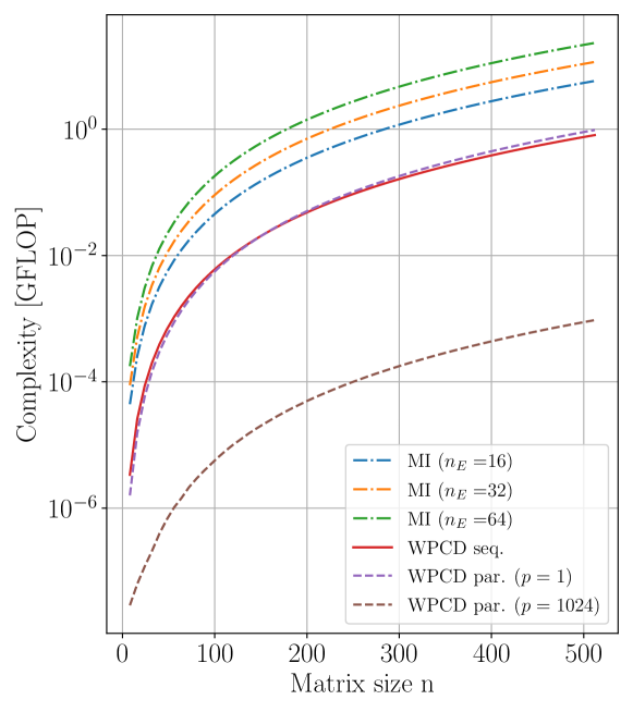
Figure 2: Complexity, as measured in FLOP, for the MI and WPCD methods as a function of $n$, where $n$ represents the number of quadrature points ($N_{\text{Q}}$) for MI and the number of wave packets ($N_{\text{WP}}$) for WPCD. Furthermore, $n_{E}$ is the number of on-shell $T$-matrix evaluations (note $n_{E}=n=N_{\text{WP}}$ for WPCD).

We see from Fig. 2 that the efficiency of the parallel WPCD approach scales very well with the number of available processors. We also see that for a single processor ($p=1$) the parallel and sequential approaches are roughly equal (while not taking into account any overhead in memory transfers), while for a realistic value $p=1024$ the complexity model for the parallel approach demonstrates a clear advantage. The value $p=1024$ corresponds to the current limit on threads with shared memory for typical Nvidia GPUs.

5 Continuum-discretised neutron-proton scattering computations

In this section we present a detailed analysis of the precision and accuracy of the WPCD method for computing neutron-proton (np) scattering observables and phase shifts. For all calculations, we employed the optimised next-to-next-to-leading-order chiral potential $\text{N2LO}_{\text{opt}}$ [48]. The primary goal is to analyse the trade-off between minimum computational cost and maximum method accuracy in the WPCD method, and contrast this to the conventional MI method. Note that there is no problem in obtaining highly accurate results from either method. We simply focus on the performance and accuracy of the WPCD method as we reduce the number of wave-packets such that all objects fit in the fast on-chip shared memory on the GPU. In our analysis we consider the MI method with $N_{\text{Q}}=96$ Gauss-Legendre points, see Eq. (4), to yield virtually exact results. For brevity, we will refer to such numerically converged calculations as exact.

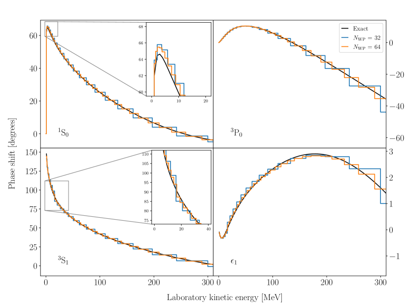
Figure 3: Phase shifts calculated using the WPCD-method using $N_{\text{WP}}$=32 (blue) and $N_{\text{WP}}$=64 (orange) wave packets. Numerically exact results (black) were obtained using the MI-method.

5.1 Computing phase shifts

In Fig. 3 we compare np scattering phase shifts in the ${}^{1}\text{S}_{0}$, ${}^{3}\text{P}_{0}$, and ${}^{3}\text{S}_{1}$ partial waves as well as the $\epsilon_{1}$ mixing angle, as obtained from the WPCD method using $N_{\text{WP}}$=32 and $N_{\text{WP}}$=64 momentum wave-packets. The free wave-packet bin boundaries follow a Chebyshev distribution with scaling factor $\alpha=100$ MeV and sparseness degree $t=2$, see Eq. (31), and the resolvent was energy-averaged according to Eq. (62).

For the WPCD-result, one immediately observes a discretised, step-like version of the otherwise smoothly varying exact description of the scattering phase shifts. This is entirely due to the momentum discretisation and finite number of wave packets. Indeed, due to the energy-averaging we obtain only one $T$-matrix element per momentum bin. In the limit $N_{\text{WP}}$$\rightarrow\infty$, and everything else equal, we will recover the exact result obtained with the MI method. We observe this convergence trend already when going from $N_{\text{WP}}$=32 to $N_{\text{WP}}$=64 wave packets. For instance, the mixing angle moves closer to the exact results when increasing $N_{\text{WP}}$. Overall, the WPCD method is performing as expected, but there are two features we would like to point out:

1. The values of the low-energy ${}^{1}\text{S}_{0}$ phase shift are overestimated near the peak where the phase shift turns over. This is likely due to the momentum-averaging of operators. The potential matrix in the ${}^{1}\text{S}_{0}$ channel ($\langle q^{\prime}|V_{{}^{1}\textrm{S}_{0}}|q\rangle$) is shown in Fig. 4 for both a continuous momentum-basis and a $N_{\text{WP}}=32$ wave-packet basis with bins distributed according to Eq. (31). The potential is constant within each wave-packet bin as expected according to Eq. (29). This makes it challenging to reproduce finer details of the interaction. There is also a discrepancy between the continuous and wave-packet values when the chosen $q^{\prime}$-momentum is not near any bra-state bin midpoint. This is most distinctive in the green curves at $q^{\prime}=205.622$ MeV, which is very close to a bin boundary. We see in Eq. (29) that we average over momenta within two bins, and when a potential varies strongly within a bin such that the matrix elements at the bin boundaries are quite different from the bin mid-point values, this averaging is too coarse to mimic the potential accurately. This effect becomes less significant with increasing $N_{\text{WP}}$ since the grid will grow denser.

   

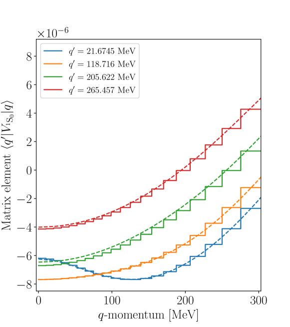
   Figure 4: The ${}^{1}\text{S}_{0}$ potential of NNLO_opt [48] as a function of $q$, at several $q^{\prime}$ values. The dashed lines represent the potential calculated in a continuous basis, while the solid lines represent a wave-packet projection. The wave-packet projection was made with an $N_{\text{WP}}=32$ basis in a Chebyshev distribution (with $\alpha=100$ MeV). In the wave-packet representation, the bra-state bin contains $q^{\prime}$. Note that the units for continuous representation of the potential is in units of MeV^-2 while the wave-packet projected potential is in units of MeV, as follows from the definition in Eq. (17).

2. The WPCD-results for ${}^{3}\text{S}_{1}$ show a distinctive drop at 90 degrees. This trend is consistent for all basis sizes and is simply due to the treatment of the deuteron bound state in the WPCD framework. We extract a phase shift $\delta$ via an inverse trigonometric function with values for $\delta\in[-90,90]$ degrees. A bound state is characterised by a transition $\delta(E+\epsilon)-\delta(E)=180$ degrees at some energy $E$ for an infinitesimal step $\epsilon>0$, as dictated by Levinson’s theorem [49]. It is apparent that this transition across 90 degrees is more difficult to reproduce for the WPCD method. The same effect also gives rise to inaccuracies in the $\epsilon_{1}$ mixing angle. However, this is of no concern when computing a scattering observable.

5.1.1 Linearly interpolating phase shifts

Although the resolution of the WPCD method is limited by the energy-averaging across each momentum-bin—i.e., yields a step-like character of the predictions—the mid-points $\bar{q}_{i}=\frac{1}{2}(q_{i-1}+q_{i})$ of each bin in Fig. 3 are typically closest to the exact results, as expected from the wave-packet eigenvalues, see Eqs. (18) and (19). We can therefore linearly interpolate the phase shifts $\delta_{i}\equiv\delta(\bar{q}_{i})$ across several bins, i.e. across scattering energies, via

$$\delta(q)=\left(\frac{\delta_{i}-\delta_{i-1}}{\bar{q}_{i}-\bar{q}_{i-1}}\right)q+\left(\delta_{i-1}-\frac{\delta_{i}-\delta_{i-1}}{\bar{q}_{i}-\bar{q}_{i-1}}\bar{q}_{i-1}\right)\>.$$ (42)

for c.m. momenta $q\in[q_{i-1},q_{i}]$ where $q_{i}$ are the FWP bin boundaries. This simple and straightforward approach offers a rather precise prediction for any on-shell scattering energy. Of course, the phase shifts can be linearly interpolated using other points, i.e. we can let

$$\bar{q}_{i}=q_{i-1}+\frac{n}{m}(q_{i}-q_{i-1})\>,$$ (43)

for some $n\in[0,m]$, such that $n=\frac{m}{2}$ is the bin mid-point again. Figure 5 shows the resulting predictions using linear (mid-point) interpolation of the ${}^{1}\text{S}_{0}$ phases presented in Fig. 3. The bands estimate the effect of varying the interpolation point. The bands span the resulting $\delta(q)$ calculated with $m=10$ and $n=[0.1,1,2,\ldots 8,9,9.9]$ in Eq. (43). As expected, mid-point interpolation yields results that are very close to the exact calculation. In the following we will therefore only use this interpolation choice.

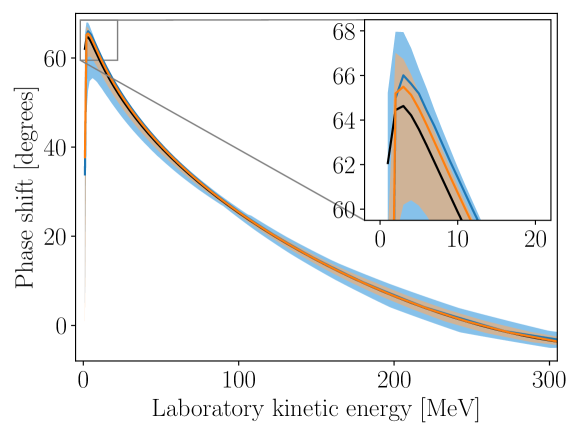
Figure 5: Phase shifts for the ${}^{1}\text{S}_{0}$ partial wave calculated using WPCD. The colour coding is the same as in Fig. 3, i.e. $N_{\text{WP}}=32$ (light blue) and $N_{\text{WP}}=64$ (light orange). The bands indicate the maximum discrepancy due to the choice of interpolation point $n$ according to Eq. (43).

5.2 Computing cross sections

We compute scattering cross sections from scattering amplitudes according to the method outlined in A. Figure 6 shows the total cross section obtained using the WPCD-method using momentum-space bins with $N_{\text{WP}}=32$ and $N_{\text{WP}}=64$. As can be seen in the figure, the linearly-interpolated results reproduce the exact result rather well. On a larger scale it is nearly impossible to tell any difference between results obtained using $N_{\text{WP}}=32$ bins and $N_{\text{WP}}=64$ bins. To emphasise the monotonically increasing accuracy of the WPCD method as we increase the number of momentum-space bins, we calculate the absolute value of the difference between the exact and the WPCD prediction for the total cross section for a range of bin resolutions, see Fig. 7. From this it is apparent that the WPCD method converges, although slowly, for a bin partition following a Chebyshev distribution.

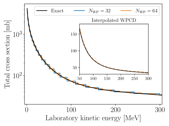
Figure 6: Total cross section calculated with the WPCD method. The solid black line corresponds to the exact result as obtained using the MI method. The inset demonstrates the high accuracy of (mid-point) interpolated WPCD results. On this scale, the two separate WPCD predictions appear to overlap completely.

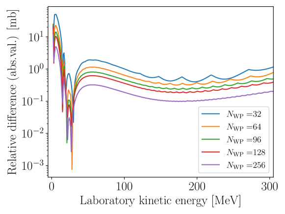
Figure 7: Absolute values of the relative difference between exact results and WPCD method for the total cross section, shown as a function of wave-packet basis size $N_{\text{WP}}$ and laboratory kinetic energy.

5.3 WPCD accuracy

There are primarily two approximations that impact the accuracy of the WPCD method: the number of bins $N_{\text{WP}}$ and the distribution thereof. Also, the averaging of continuous states into wave packets means we use momentum-averaged matrix representations of operators in the LS equation. This averaging should improve with reduced bin widths. We can easily control $N_{\text{WP}}$, and in this section we analyse the performance of WPCD with respect to different choices of this method parameter.

To better quantify the convergence of the WPCD method we study the root-mean-square error (RMSE) with respect to the exact result for the total cross section across a range of scattering energies. We use the standard RMSE measure

$$\text{RMSE}=\sqrt{\frac{\sum_{i=1}^{n_{E}}\left(\sigma_{\text{exact},i}-\sigma_{\text{method},i}\right)^{2}}{n_{E}}}\>,$$ (44)

where $\sigma_{\text{exact},i}$ denotes the exact results and $\sigma_{\text{method},i}$ denotes either the WPCD- or MI-calculated total cross sections at some scattering energy $E_{i}$ for $i=1,\ldots,n_{E}$.

We find that the RMSE for WPCD with scattering energies corresponding to laboratory kinetic energies $40\leq T_{\rm lab}\leq 350$ MeV remains fairly constant at $\sim 2.0$ mb when using $N_{\text{WP}}=16$. This is interesting for three reasons:

• The WPCD coupled channel Hamiltonian will be of size $2N_{\text{WP}}\times 2N_{\text{WP}}$, i.e. we diagonalise $32\times 32$ Hamiltonian matrices. Most GPUs today, including the Nvidia Tesla V100 we have used here, have 64 kB shared memory (also called “on-chip” memory) which is significantly faster to access than the GPU’s main memory. These matrices fit entirely on the GPU shared memory, allowing for a strong reduction in GPU memory read/write demand while performing the diagonalisation.

• A recent Bayesian analysis of chiral interactions suggests that the $\chi$EFT truncation error for scattering cross sections at next-to-next-to-leading-order is at least 2 mb, at 68% degree-of-belief (DoB), and at least 5 mb at 95% DoB [20].

• Regarding experimental uncertainties, the combined statistical and systematic uncertainties in measured np total cross sections are at the 1% level [50, 51]. In absolute terms, this amounts to uncertainties of the order $1$ mb at laboratory scattering energies $\gtrsim 40$ MeV. At lower energies the cross section increases of course, leading to slightly larger absolute experimental errors.

In summary, we find that the WPCD method error, when using very few wave-packets, is slightly larger than typical experimental uncertainties but smaller than the estimated model discrepancy up to next-to-next-to-leading-order in $\chi$EFT.

One can clearly reduce the WPCD method error by increasing $N_{\rm WP}$. However, this will also increase the computational cost and we recommend studying the actual wall time cost in relation to, e.g. the RMSE measure defined above. We perform such an analysis in Sec. 6.

Before ending this section on the method accuracy, we would like to emphasise that the maximum total angular momentum $J_{\text{max}}$ in the partial-wave expansion of the potential also impacts the accuracy of the description of the scattering amplitude. For the linearly-interpolated WPCD method with $N_{\text{WP}}=16$, where we observe a method error of $\sim 2$ mb in the total cross section at $T_{\rm Lab}\gtrsim 40$ MeV, and find it unnecessary to go beyond $J_{\rm max}=6$.

6 Method Performance

With an account of the precision and accuracy of the WPCD method we now profile its time performance. Typically, when using the MI method, we calculate every on-shell phase shift of interest by explicitly solving the LS equation, while in the WPCD approach we interpolate in-between bin mid-points, as discussed above. This will, unsurprisingly, induce a substantial time-performance penalty in using the MI method, due to the linear scaling with the number of energy solutions, as shown in Eq. (37). However, we can of course linearly interpolate the phase shifts calculated with the MI method, rather than invoking an explicit calculation at every on-shell energy. Therefore, to facilitate a balanced comparison between the two methods, we also employed linear interpolation to extract phase shifts when using the MI method. In our studies, this has turned out to be a highly efficient way to speed up the calculation with the MI method while maintaining precision and accuracy of the results.

To facilitate a comparison, when using the MI method we solve the LS equation at $n_{E}$ on-shell energies also following a Chebyshev distribution. We then linearly interpolate the phase shifts using these energies to calculate neutron-proton total cross sections in the $T_{\rm lab}$ energy ranges $(0,350]$ MeV and $(40,350]$ MeV for the calculation of RMSE values.

For WPCD we can only vary the number of wave packets $N_{\rm WP}$ while for MI we can vary both $N_{\text{Q}}$ and $n_{E}$, i.e. the number quadrature points and the number of interpolation points or on-shell energies (at bin mid-points), respectively. Figure 8 shows the wall times for solving the LS equation to obtain cross sections, at different levels of method accuracy measured by the RMSE value. In Tab. 1 we show a few interpretations of the figure for a handful of relevant method parameters. As mentioned, the WPCD method is implemented on a GPU while the MI results were obtained using an optimised CPU implementation [7]. The time profiles were obtained using an Nvidia Tesla V100 32 GB SMX2 and an Intel Xeon Gold 6130 for the WPCD GPU and MI CPU results, respectively.

From our analysis we conclude that the WPCD method is faster than the MI method if one can tolerate $\sim 1-5$ mb method RMSE in the prediction of total scattering cross sections. For such applications it would then be advisable to use $N_{\text{WP}}\gtrsim 48$ bins, on the basis of Fig. 8. It is worth noting that the RMSE is dominated by contributions from scattering cross sections below laboratory kinetic energies $T_{\rm lab}\sim 40$ MeV. Indeed, with $N_{\rm WP}=48$ we obtain an RMSE value of $\sim 4$ mb across an interval $T_{\rm lab}\in(0,350]$ MeV. The RMSE drops to $\sim 0.8$ mb when considering only cross sections with $T_{\rm lab}>40$ MeV. Irrespective of how the WP bins are distributed, it is therefore necessary to ensure a sufficiently high density of bins below $T_{\text{lab}}=40$ MeV to accurately reproduce the ${}^{1}\text{S}_{0}$ phase-shift peak and the ${}^{3}\text{S}_{1}$ bound state. With the WPCD method we can obtain increasingly faster solutions to the LS equation as we reduce the number of wave-packets.

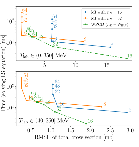
Figure 8: Measured wall times for solving the LS equation for different values of total cross section RMSE for $T_{\text{lab}}\in(0,350]$ MeV (top panel) and $T_{\text{lab}}\in(40,350]$ MeV (bottom panel). $n_{E}$ is the number of on-shell energies (interpolation points) at WP bin mid-points, according to a Chebyshev distribution. The numeric label attached to each data point indicates the number of Gauss-Legendre grid points $N_{\text{Q}}$ for the MI method and the number of wave packets $N_{\text{WP}}$ for the WPCD method. The number of energies used for interpolating the MI results are indicated in the legend. See the main text for hardware specifications.

Table 1: Measured wall times, corresponding to the results in Fig. 8, for solving the LS equation and predicting total cross sections using the WPCD and MI methods, at different RMSE levels in the $T_{\text{lab}}\in(40,350]$ MeV energy region. The $n_{E}$ parameter indicates the number of interpolation energies used for the MI method.

RMSE [mb]	MI			WPCD
	$N_{\text{Q}}$	$n_{E}$	Time [ms]	$N_{\text{WP}}$	Time [ms]
3.0	8	16	6	–	–
2.5	$10$	16	7	–	–
2.0	$12$	16	8	16	0.5
1.5	$14$	16	10	$24$	2.5
1.0	$16$	$24$	$15$	32	6
0.5	16	32	20	96	$35$

7 Summary and outlook

In this study we have compared the WPCD method with the standard MI method, with an emphasis on their respective efficiency, precision, and accuracy when solving NN scattering problems. This study is done with an interest in reducing the computational costs of Bayesian inference analyses of nuclear interaction models.

We find that the WPCD method, with GPU-acceleration, is capable of providing scattering solutions to the NN LS equation much faster than a conventional MI method implemented on a CPU. This is largely due to the WPCD method being capable of delivering scattering amplitudes at several on-shell energies in an inherently parallel fashion, and that linear interpolation across several WP bins offers straightforward predictions for any scattering energy. However, compared to solutions obtained using the standard MI method, the WPCD method is less accurate, in particular in regions where the scattering amplitudes vary strongly with energy. This is also expected due to the momentum-space discretisation and approximation of the scattering states. Nevertheless, in applications where a certain method error can be tolerated—as for example in low-order EFT predictions of NN scattering cross sections—the GPU-implemented WPCD method presents a computational advantage. This finding makes it particularly promising for computational statistics analyses of EFT nuclear interactions utilising Bayesian inference methods.

We also find that the computational gain of using GPU hardware is limited by the amount of shared memory that is available. This constraint basically corresponds to an upper limit on the number of WP bins that can be used for efficient computations. We note, however, that GPU hardware is continuously improved, and that a four-fold increase in the size of the fast shared memory on the GPU would enable a two-fold increase of both the WP-basis and method accuracy while incurring a very mild additional computational cost. The GPU global memory is typically not saturated in WPCD calculations of NN scattering calculations. The WPCD method can also be applied to compute three-nucleon scattering amplitudes [37, 52]. However, the limited amount of global memory might become a constraining factor for such applications that involve a more complicated Hilbert space basis.

In this study we have focused on the inherent parallelism of the WPCD method and the opportunities that it offers to benefit from the use of GPU hardware. Of course, one could also explore parallelisation of the WPCD method on a CPU and make parallel use of the fast cores available in modern CPUs. The efficiency of the GPU WPCD approach is almost fully determined by the time needed to diagonalize the channel Hamiltonian and could therefore benefit from the faster CPU clock speed. Naturally, one could also consider a GPU implementation of the MI method wherein the LS equation is solved in a parallel fashion for multiple scattering energies simultaneously. Still, this would require multiple matrix inversions (one for each interpolation energy). A simple phase-shift interpolation applied to the MI method facilitates sufficiently accurate results for NN scattering observables, at a significantly lower computational cost compared to explicitly solving the LS equation at every scattering energy of interest.

Appendix A Scattering cross sections and the spin-scattering matrix

A scattering observable of some operator $\hat{O}$ can generally be written as a trace [28],

$$\langle\hat{O}\rangle=\frac{\text{Tr}\{M\hat{\rho}_{i}M^{\dagger}\hat{O}\}}{\text{Tr}\{M\hat{\rho}_{i}M^{\dagger}\}}\>,$$ (45)

where $\hat{\rho}$ is the spin-density matrix, usually represented in a helicity basis, and $M$ is the spin-scattering matrix.

The helicity-basis projection of the spin-scattering matrix is written as $M_{m_{s},m_{s^{\prime}}}^{s}$, where $s$ is the conserved total spin and $m_{s}$ is the corresponding projected spin. These matrices are usually expressed in partial-wave expansions,

$$\begin{split}M_{m_{s},m_{s^{\prime}}}^{s}=\frac{2\pi}{ip}\sum_{J,l,l^{\prime}}&[1-(-1)^{l+s+T_{Z}}]\sqrt{\frac{2l+1}{4\pi}}\\ &\times Y_{m_{s}-m_{s^{\prime}}}^{l^{\prime}}(\theta,\phi)\\ &\times\langle l^{\prime},s,m_{s}-m_{s^{\prime}},m_{s^{\prime}}|l^{\prime},s^{\prime},j,m_{s}\rangle\\ &\times\langle l,s,m_{s},0|l,s,j,m_{s}\rangle\\ &\times\left[S^{1J}_{l^{\prime}l}(p^{\prime},p)-\delta_{l,l^{\prime}}\right]\>,\end{split}$$ (46)

where the third and fourth rows are Clebsch-Gordan coefficients, $J$ is the total angular momentum, $l$ and $l^{\prime}$ are the orbital angular momenta of the inbound and outbound states respectively, $T_{Z}$ is the azimuthal isospin projection, $Y_{m}^{l}(\theta,\phi)$ is an azimuthal spherical harmonic, and $S^{1J}_{l^{\prime}l}(p^{\prime},p)=\langle p^{\prime},l^{\prime},s,J|S|p,l,s,J\rangle$ is the usual scattering matrix.

The on-shell partial-wave-projected $S$-matrix is related to the on-shell $T(p,p;E)$-matrix element via

$$S^{sJ}_{l^{\prime}l}(p,p;E)=1-2\pi iT^{sJ}_{l^{\prime}l}(p,p;E)\>.$$ (47)

Due to the conservation of probability, the $S$-matrix is unitary, and can therefore be parametrised by real parameters like phase shifts. In the Stapp convention [53], the coupled-channel $S$-matrix $S^{1J}_{l^{\prime}l}$ is then given by

$$S=\begin{pmatrix}\cos(2\epsilon_{J})e^{2i\delta_{-,J}}&i\sin(2\epsilon_{J})e^{i(\delta_{-,J}+\delta_{+,J})}\\ i\sin(2\epsilon_{J})e^{i(\delta_{-,J}+\delta_{+,J})}&\cos(2\epsilon_{J})e^{2i\delta_{+,J}}\end{pmatrix}\>,$$ (48)

where $\delta_{\pm,J}$ refers to $\delta_{l,J}$ for $l=J\pm 1$ and $\epsilon_{J}$ is the mixing angle. The uncoupled-channel $S$-matrix $S^{0J}_{ll}$ is given by (for $l=J$)

$$S=e^{2i\delta_{J,J}}\>.$$ (49)

The angle $\theta$ denotes the scattering angle between the c.m. inbound and outbound relative momenta $\bm{p}$ and $\bm{p}^{\prime}$ respectively, while $\phi$ is the rotation angle of $\bm{p}^{\prime}$ around the inbound momentum $\bm{p}$, but cylindrical symmetry allows us to set $\phi=0$. Using Eq. (46) we can calculate scattering observables such as the differential cross section,

$$\frac{d\sigma}{d\Omega}=\frac{1}{4}\text{Tr}(MM^{\dagger})\>.$$ (50)

However, this approach does not utilise symmetries to reduce the number of non-contributing terms of $M_{m_{s},m_{s^{\prime}}}^{s}$. Instead, the $M$-matrix can be expressed in terms of non-vanishing spin-momentum products after some consideration of parity conservation, isospin and time-reversal symmetries, and the Pauli principle. We use the Saclay convention [54] for these terms,

$$\begin{split}M=\frac{1}{2}\big{[}(a+b)&+(a-b)(\bm{\sigma}_{1}\cdot\bm{n})(\bm{\sigma}_{2}\cdot\bm{n})\\ &+(c+d)(\bm{\sigma}_{1}\cdot\bm{m})(\bm{\sigma}_{2}\cdot\bm{m})\\ &+(c-d)(\bm{\sigma}_{1}\cdot\bm{l})(\bm{\sigma}_{2}\cdot\bm{l})\\ &+e((\bm{\sigma}_{1}+\bm{\sigma}_{2})\cdot\bm{m})\big{]}\>,\end{split}$$ (51)

where $a,b,c,d$, and $e$ are the Saclay amplitudes, $\bm{\sigma}_{i}$ are the Pauli spin matrices acting on nucleon $i=1,2$, and where we define the following unit vectors

$$\bm{l}\equiv\frac{\bm{p}+\bm{p}^{\prime}}{|\bm{p}+\bm{p}^{\prime}|}\>,\>\>\bm{m}\equiv\frac{\bm{p}-\bm{p}^{\prime}}{|\bm{p}-\bm{p}^{\prime}|}\>,\>\>\bm{n}\equiv\frac{\bm{p}\times\bm{p}^{\prime}}{|\bm{p}\times\bm{p}^{\prime}|}\>.$$ (52)

The Saclay amplitudes are given by the spin-projected matrices as,

$$\begin{split}a&=\frac{1}{2}(M^{1}_{11}+M^{1}_{0,0}+M^{1}_{1,-1})\>,\\ b&=\frac{1}{2}(M^{1}_{11}+M^{0}_{0,0}+M^{1}_{1,-1})\>,\\ c&=\frac{1}{2}(M^{1}_{11}-M^{0}_{0,0}+M^{1}_{1,-1})\>,\\ d&=-\frac{1}{\sqrt{2}\sin(\theta)}(M^{1}_{1,0}+M^{1}_{0,1})\>,\\ e&=\frac{i}{2\sqrt{2}}(M^{1}_{1,0}-M^{1}_{0,1})\>.\end{split}$$ (53)

In this parametrisation, the differential cross-section is given by

$$\frac{d\sigma}{d\Omega}=\frac{1}{2}\left(|a|^{2}+|b|^{2}+|c|^{2}+|d|^{2}+|e|^{2}\right)\>.$$ (54)

For the results in this paper we used the following expression for the total cross section:

$$\sigma_{\text{tot}}=\frac{2\pi}{p}\text{Im}(a+b)\>.$$ (55)

See Ref. [54] for a complete account of scattering observables in the Saclay parametrisation.

Appendix B The resolvent in a wave-packet basis

The resolvent $\hat{g}(E)$ for the full Hamiltonian $\hat{h}\equiv\hat{h}_{0}+\hat{v}$,

$$\hat{g}(E)\equiv\frac{1}{E-\hat{h}\pm i\epsilon}\>,$$ (56)

can be calculated analytically in a pseudostate wave-packet basis $\{|z_{i}\rangle\}_{i=1}^{n}$ of the full Hamiltonian. The resolvent is represented in the basis by (see Eq. (17))

$$\begin{split}\langle z_{i}|\hat{g}(E)|z_{j}\rangle&=\langle z_{i}|\frac{1}{E-\hat{h}\pm i\epsilon}|z_{j}\rangle\\ &=\frac{1}{\mu\sqrt{N_{i}N_{j}}}\int_{\mathcal{D}_{i}}\int_{\mathcal{D}_{j}}\mathop{}\!\mathrm{d}k^{\prime}\mathop{}\!\mathrm{d}k\\ &\hskip 56.9055pt\times\frac{k^{\prime}k\sqrt{k^{\prime}k}\langle\psi_{k^{\prime}}^{(+)}|\psi_{k}^{(+)}\rangle}{E-\frac{k^{\prime 2}}{2\mu}\pm i\epsilon}\>,\end{split}$$ (57)

where $\mu=\frac{m_{N}}{2}$. Note that we set the weight function $f(k)=\sqrt{\frac{k}{\mu}}$ and normalisation $N_{i}=\Delta\mathcal{E}_{i}$ as these are energy wave-packets (from the diagonalisation of $\hat{h}$). Using $\langle\psi_{k^{\prime}}^{(+)}|\psi_{k}^{(+)}\rangle=\frac{\delta(k^{\prime}-k)}{k^{\prime}k}$, this becomes

$$\langle z_{i}|\hat{g}(E)|z_{j}\rangle=\frac{\delta_{ij}}{\mu N_{i}}\int_{\mathcal{D}_{i}}\mathop{}\!\mathrm{d}k\>\frac{k}{E-\frac{k^{2}}{2\mu}\pm i\epsilon}\>,$$ (58)

where we have introduced the Kronecker delta $\delta_{ij}$ since $\langle\psi_{k^{\prime}}^{(+)}|\psi_{k}^{(+)}\rangle=0\>\forall\>\mathcal{D}_{i}\neq\mathcal{D}_{j}$. For positive energies, where $E=\frac{p^{2}}{2\mu}$ and where $p$ is the on-shell c.m. momentum, we get

$$\langle z_{i}|\hat{g}(E)|z_{j}\rangle=\frac{2\delta_{ij}}{D_{i}}\int_{\mathcal{D}_{i}}\mathop{}\!\mathrm{d}k\>\frac{k}{p^{2}-k^{2}\pm i\epsilon}\>,$$ (59)

If $E\notin\mathcal{D}_{i}$, we take the limit $\epsilon\rightarrow 0$ and solve the integral to find

$$\begin{split}\langle z_{i}|\hat{g}(E)|z_{j}\rangle&=\frac{2\delta_{ij}}{N_{i}}\int_{\mathcal{D}_{i}}\mathop{}\!\mathrm{d}k\>\frac{k}{p^{2}-k^{2}}\\ &=\frac{\delta_{ij}}{N_{i}}\left[-\ln\left|\frac{k^{2}}{p^{2}}-1\right|\right]_{k_{i}}^{k_{i+1}}\\ &=\frac{\delta_{ij}}{N_{i}}\ln\left|\frac{E+\mathcal{E}_{i+1}}{E+\mathcal{E}_{i}}\right|\>,\end{split}$$ (60)

where $p\notin\mathcal{D}_{i}$, and $\mathcal{E}_{i}$ and $\mathcal{E}_{i+1}$ is the lower and upper boundary of $\mathcal{D}_{i}$ expressed in energy, respectively. If $E\in\mathcal{D}_{i}$, then we have a simple pole at $p=k$. The pole-integration is done using the infinitesimal complex rotation $\pm i\epsilon$ together with the residue theorem, giving

$$\begin{split}\langle z_{i}|\hat{g}(E)|z_{j}\rangle=\frac{\delta_{ij}}{N_{i}}\bigg{[}&\ln\left|\frac{E+\mathcal{E}_{i+1}}{E+\mathcal{E}_{i}}\right|\\ &-i\pi(\theta(E-\mathcal{E}_{i})-\theta(E-\mathcal{E}_{i+1}))\bigg{]}\>,\end{split}$$ (61)

where $\theta$ is the Heaviside step-function. The derivation of the resolvent expressed in a momentum wave-packet representation follows a similar procedure. In that case, it is possible to use momentum wave-packets where $f(p)=1$ and $N_{i}=\sqrt{k_{i+1}-k_{i}}$, in which case the derivation above changes a little, see [18].

Energy averaging of the resolvent is done by integrating the resolvent with respect to $E$, in the bin $E\in\mathcal{D}_{k}$, divided by the bin width $\Delta\mathcal{E}_{k}$. We introduce the denotation $\bar{g}_{ij}^{k}$ to reflect this. The derivation is straightforward:

$$\begin{split}\bar{g}_{ij}^{k}&\equiv\frac{1}{\Delta\mathcal{E}_{k}}\int_{\mathcal{D}_{k}}\mathop{}\!\mathrm{d}E\>\langle z_{i}|\hat{g}(E)|z_{j}\rangle\\ &=\frac{\delta_{ij}}{\Delta\mathcal{E}_{k}N_{i}}\int_{\mathcal{D}_{k}}\mathop{}\!\mathrm{d}E\>\left[\ln\left|\frac{E+\mathcal{E}_{i+1}}{E+\mathcal{E}_{i}}\right|-i\pi\delta_{ik}\right]\\ &=\frac{\delta_{ij}}{\Delta\mathcal{E}_{k}\Delta\mathcal{E}_{i}}W_{ki}-\frac{i\pi}{\Delta\mathcal{E}_{k}}\delta_{ik}\>,\end{split}$$ (62)

where we used $N_{i}=\Delta\mathcal{E}_{i}$, and

$$W_{ki}\equiv\sum_{k^{\prime}=k}^{k+1}\sum_{i^{\prime}=i}^{i+1}(-1)^{k-k^{\prime}+i-i^{\prime}}\left[\mathcal{E}_{k^{\prime}}-\mathcal{E}_{i^{\prime}}\right]\ln\left|\mathcal{E}_{k^{\prime}}-\mathcal{E}_{i^{\prime}}\right|\>.$$ (63)

as presented in [18].

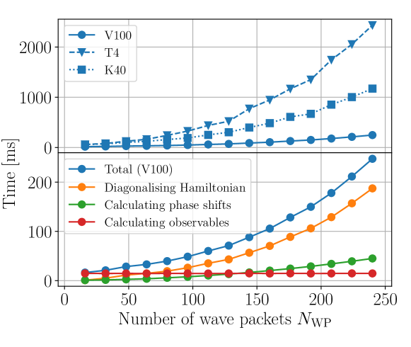
Figure 9: Top: total time used in calculating on-shell $T$-matrix elements and extracting phase shifts and observables, shown for three different Nvidia GPUs of the Tesla line; T4 (orange), V100 (blue), and K40 (green). Bottom: time decomposition of V100 total time, with focus on key parts of calculating NN scattering using the WPCD method. The green line includes the time spent solving the LS equation.

Appendix C GPU code

The code for GPU-utilisation was written to make use of the CUDA interface, which is developed and maintained by the Nvidia Corporation. CUDA allows for efficient utilisation of a Nvidia GPU using high-level programming languages such as C and C++, Python, or Fortran. For numerically demanding linear algebra operations we made use of the CUDA-libraries cuBLAS[42] and cuSOLVER[43]. These libraries are very similar in use to BLAS and LAPACK—two standard libraries for linear algebra on the CPU.

Diagonalising the full Hamiltonian and solving the LS equation are the most numerically demanding parts of the steps presented in Sec. 3.2. These steps are therefore solved on the GPU. The ability to work on several channels simultaneously—this being the advantage of the GPU—is made possible by using CUDA’s batched-routines. These are pre-written routines that maximise the efficiency of the GPU to solve several linear algebra problems simultaneously for small matrix-sizes (typically less than $1000\times 1000$ in matrix dimension). Such efficient parallelism is generally difficult to achieve “by hand”due to the massive load on GPU-memory read-write accesses.

The importance of efficient memory use is made apparent in Fig. 9 where we show the computation time spent by three different Nvidia GPUs (top panel) and the decomposition of time used for the Nvidia V100 GPU (bottom panel). We see that the majority of the total time is spent on the Hamiltonian diagonalisation. A large fraction of the diagonalisation task is spent on memory accesses as part of the Jacobi method. The three GPUs: V100, T4, and K40, have differences in memory technology [55] which is the main reason for the observed differences in the performance.

We usedcublas<t>gemmStridedBatched to calculate the $VC$-matrix product in Eq. (32). This calculates a matrix-product on the form $C\leftarrow\alpha AB+\beta C$, where $C$ is overwritten by the right-hand side. This setup is standard for BLAS gemm-routines. Here, $\alpha$ and $\beta$ are scalars, while $A$, $B$, and $C$ are sets of matrices stored congruently in three arrays, i.e. they are “batched”.

To diagonalise the Hamiltonians we used cusolverDn<t>syevjBatched. This routine utilises the parallel cyclic-order Jacobi method, as was briefly discussed in Sec. 4.2, to diagonalise batches of matrices simultaneously.

Lastly, solving Eq. (39) was done using a custom-written function, referred to as a “kernel” in CUDA. The advantage of using the GPU for this task comes with the energy-dependence in the resolvent. We can calculate all on-shell $T$-matrix elements simultaneously following a single batched Hamiltonian diagonalisation.

References

References

- [1] P. F. Bedaque and U. van Kolck. Effective field theory for few-nucleon systems. Annu. Rev. Nucl. Part. Sci., 52(1):339–396, 2002.
- [2] E. Epelbaum, H.-W. Hammer, and Ulf-G. Meißner. Modern theory of nuclear forces. Rev. Mod. Phys., 81:1773–1825, 12 2009.
- [3] R. Machleidt and D. R. Entem. Chiral effective field theory and nuclear forces. Phys. Rep., 503(1):1 – 75, 2011.
- [4] H.-W. Hammer, Sebastian König, and U. van Kolck. Nuclear effective field theory: Status and perspectives. Rev. Mod. Phys., 92:025004, Jun 2020.
- [5] S. Wesolowski, N. Klco, R. J. Furnstahl, D. R. Phillips, and A. Thapaliya. Bayesian parameter estimation for effective field theories. J. Phys. G, 43(7):074001, may 2016.
- [6] D. R. Entem and R. Machleidt. Accurate charge-dependent nucleon-nucleon potential at fourth order of chiral perturbation theory. Phys. Rev. C, 68:041001, Oct 2003.
- [7] B. D. Carlsson, A. Ekström, C. Forssén, D. Fahlin Strömberg, G. R. Jansen, O. Lilja, M. Lindby, B. A. Mattsson, and K. A. Wendt. Uncertainty analysis and order-by-order optimization of chiral nuclear interactions. Phys. Rev. X, 6:011019, 2 2016.
- [8] P. Reinert, H. Krebs, and E. Epelbaum. Semilocal momentum-space regularized chiral two-nucleon potentials up to fifth order. Eur. Phys. J. A, 54(5):86, 2018.
- [9] M. Piarulli, L. Girlanda, R. Schiavilla, R. Navarro Pérez, J. E. Amaro, and E. Ruiz Arriola. Minimally nonlocal nucleon-nucleon potentials with chiral two-pion exchange including resonances. Phys. Rev. C, 91:024003, Feb 2015.
- [10] R. Navarro Pérez, J. E. Amaro, and E. Ruiz Arriola. Coarse-grained potential analysis of neutron-proton and proton-proton scattering below the pion production threshold. Phys. Rev. C, 88:064002, Dec 2013.
- [11] Dillon Frame, Rongzheng He, Ilse Ipsen, Daniel Lee, Dean Lee, and Ermal Rrapaj. Eigenvector continuation with subspace learning. Phys. Rev. Lett., 121(3):032501, 2018.
- [12] S. König, A. Ekström, K. Hebeler, D. Lee, and A. Schwenk. Eigenvector Continuation as an Efficient and Accurate Emulator for Uncertainty Quantification. Phys. Lett. B, 810:135814, 2020.
- [13] R. J. Furnstahl, A. J. Garcia, P. J. Millican, and X. Zhang. Efficient emulators for scattering using eigenvector continuation. Phys. Lett. B, 809:135719, 2020.
- [14] J. A. Melendez, C. Drischler, A. J. Garcia, R. J. Furnstahl, and Xilin Zhang. Fast & accurate emulation of two-body scattering observables without wave functions. 6 2021.
- [15] Xilin Zhang and R. J. Furnstahl. Fast emulation of quantum three-body scattering, 2021.
- [16] Carl Edward Rasmussen and Christopher K. I. Williams. Gaussian Processes for Machine Learning (Adaptive Computation and Machine Learning). The MIT Press, 2005.
- [17] M. I. Haftel and F. Tabakin. Nuclear saturation and the smoothness of nucleon-nucleon potentials. Nucl. Phys. A, 158(1):1 – 42, 1970.
- [18] O. A. Rubtsova, V. I. Kukulin, and V. N. Pomerantsev. Wave-packet continuum discretization for quantum scattering. Ann. Phys. (N. Y.), 360:613–654, 2015.
- [19] J. Brynjarsdóttir and A. O’Hagan. Learning about physical parameters: the importance of model discrepancy. Inverse Probl., 30(11):114007–25, October 2014.
- [20] J. A. Melendez, S. Wesolowski, and R. J. Furnstahl. Bayesian truncation errors in chiral effective field theory: Nucleon-nucleon observables. Phys. Rev. C, 96:024003, 8 2017.
- [21] L. Hulthén. Kungl. Fysiogr. Sällsk. i Lund Förhandl., 14, 1944.
- [22] L. Hulthén. Arkiv Mat. Astron. Fysik, 35A, 1948.
- [23] W. Kohn. Variational methods in nuclear collision problems. Phys. Rev., 74:1763–1772, Dec 1948.
- [24] C. Schwartz. Application of the schwinger variational principle for scattering. Phys. Rev., 141:1468–1470, Jan 1966.
- [25] J. L. Basdevant. The padé approximation and its physical applications. Fortschr. Phys., 20(5):283–331, 1972.
- [26] K. Erkelenz, R. Alzetta, and K. Holinde. Momentum space calculations and helicity formalism in nuclear physics. Nucl. Phys. A, 176:413–432, 1971.
- [27] J. J. du Croz and N. J. Higham. Stability of Methods for Matrix Inversion. IMA J. Numer. Anal., 12(1):1–19, 1 1992.
- [28] W. Glöckle. The quantum mechanical few-body problem. Springer Science & Business Media, 2012.
- [29] J. Carbonell, A. Deltuva, A. C. Fonseca, and R. Lazauskas. Bound state techniques to solve the multiparticle scattering problem. Prog. Part. Nucl. Phys., 74:55 – 80, 2014.
- [30] E. J. Heller. Theory of -matrix green’s functions with applications to atomic polarizability and phase-shift error bounds. Phys. Rev. A, 12:1222–1231, Oct 1975.
- [31] J. R. Winick and W. P. Reinhardt. Moment -matrix approach to -h scattering. i. angular distribution and total cross section for energies below the pickup threshold. Phys. Rev. A, 18:910–924, Sep 1978.
- [32] J. R. Winick and W. P. Reinhardt. Moment -matrix approach to -h scattering. ii. elastic scattering and total cross section at intermediate energies. Phys. Rev. A, 18:925–934, Sep 1978.
- [33] E. J. Heller, T. N. Rescigno, and W. P. Reinhardt. Extraction of scattering information from fredholm determinants calculated in an basis: A chebyschev discretization of the continuum. Phys. Rev. A, 8:2946–2951, Dec 1973.
- [34] C. T. Corcoran and P. W. Langhoff. Moment‐theory approximations for nonnegative spectral densities. J. Math. Phys., 18(4):651–657, 1977.
- [35] O. A. Rubtsova and V. I. Kukulin. Wave-packet discretization of a continuum: Path toward practically solving few-body scattering problems. Phys. At. Nucl., 70(12):2025–2045, Dec 2007.
- [36] V. I. Kukulin, V. N. Pomerantsev, and O. A. Rubtsova. Wave-packet continuum discretization method for solving the three-body scattering problem. Theor. Math. Phys., 150(3):403–424, Mar 2007.
- [37] O. A. Rubtsova, V. N. Pomerantsev, and V. I. Kukulin. Quantum scattering theory on the momentum lattice. Phys. Rev. C, 79:064602, 6 2009.
- [38] V. I. Kukulin and O. A. Rubtsova. Discrete quantum scattering theory. Theor. Math. Phys., 134(3):404–426, Mar 2003.
- [39] H. Müther, O. A. Rubtsova, V. I. Kukulin, and V. N. Pomerantsev. Discrete wave-packet representation in nuclear matter calculations. Phys. Rev. C, 94:024328, 8 2016.
- [40] V. I. Kukulin and O. A. Rubtsova. Solving the Charged-Particle Scattering Problem by Wave Packet Continuum Discretization. Theor. Math. Phys., 145:1711––1726, Dec 2005.
- [41] O. A. Rubtsova, V. I. Kukulin, V. N. Pomerantsev, and A. Faessler. New approach toward a direct evaluation of the multichannel multienergy matrix without solving the scattering equations. Phys. Rev. C, 81:064003, Jun 2010.
- [42] Dense linear algebra on gpus. https://developer.nvidia.com/cublas, 2021. Accessed: 2021-03-22.
- [43] Cuda toolkit documentation. https://docs.nvidia.com/cuda/cusolver/index.html, 2021. Accessed: 2021-03-22.
- [44] G. H. Golub and C. F. Van Loan. Matrix Computations. The Johns Hopkins University Press, Baltimore, MD, USA, third edition, 1996.
- [45] M. Pourzandi and B. Tourancheau. A parallel performance study of jacobi-like eigenvalue solution. Technical Report, 05 1994.
- [46] A. Abdelfattah, S. Tomov, and J. Dongarra. Matrix multiplication on batches of small matrices in half and half-complex precisions. J. Parallel Distrib. Comput., 145:188 – 201, 2020.
- [47] S. E. Bae, T.-W. Shinn, and T. Takaoka. A faster parallel algorithm for matrix multiplication on a mesh array. Procedia Comput. Sci., 29:2230 – 2240, 2014. 2014 International Conference on Computational Science.
- [48] A. Ekström, G. Baardsen, C. Forssén, G. Hagen, M. Hjorth-Jensen, G. R. Jansen, R. Machleidt, W. Nazarewicz, T. Papenbrock, J. Sarich, and S. M. Wild. Optimized chiral nucleon-nucleon interaction at next-to-next-to-leading order. Phys. Rev. Lett., 110:192502, 5 2013.
- [49] N. Levinson. On the uniqueness of the potential in a schrodinger equation for a given asymptotic phase. Kgl. Danske Videnskab Selskab. Mat. Fys. Medd., 25(9), 1 1949.
- [50] P. W. Lisowski, R. E. Shamu, G. F. Auchampaugh, N. S. P. King, M. S. Moore, G. L. Morgan, and T. S. Singleton. Search for resonance structure in the total cross section below 800 mev. Phys. Rev. Lett., 49:255–259, Jul 1982.
- [51] W. P. Abfalterer, F. B. Bateman, F. S. Dietrich, R. W. Finlay, R. C. Haight, and G. L. Morgan. Measurement of neutron total cross sections up to 560 mev. Phys. Rev. C, 63:044608, Mar 2001.
- [52] V. N. Pomerantsev, V. I. Kukulin, and O. A. Rubtsova. New general approach in few-body scattering calculations: Solving discretized Faddeev equations on a graphics processing unit. Phys. Rev. C, 89(6):064008, 2014.
- [53] H. P. Stapp, T. J. Ypsilantis, and N. Metropolis. Phase-shift analysis of 310-mev proton-proton scattering experiments. Phys. Rev., 105:302–310, 1 1957.
- [54] J. Bystricky, F. Lehar, and P. Winternitz. Formalism of nucleon-nucleon elastic scattering experiments. J. Phys. France, 39(1):1–32, 1978.
- [55] Z. Jia, M. Maggioni, J. Smith, and D. P. Scarpazza. Dissecting the nvidia turing t4 gpu via microbenchmarking, 2019.