Parallelized Computation and Backpropagation Under Angle-Parametrized Orthogonal Matrices

Abstract

We present a methodology for parallel acceleration of learning in the presence of matrix orthogonality and unitarity constraints of interest in several branches of machine learning. We show how an apparently sequential elementary rotation parametrization can be restructured into blocks of commutative operations using a well-known tool for coloring the edges of complete graphs, in turn widely applied to schedule round-robin (all-against-all) sports tournaments. The resulting decomposition admits an algorithm to compute a fully-parametrized orthogonal matrix from its rotation parameters in $O(n)$ sequential steps and one to compute the gradient of a training loss with respect to its parameters in $O(n\log n)$ steps. We discuss parametric restrictions of interest to generative modeling and present promising performance results with a prototype GPU implementation.

1 Introduction

We consider in this paper the task of accelerating learning with generic orthogonal and unitary matrices via parallel implementation. More specifically, we first observe how a common parametrization of such matrices of size $n$ as a composition of $O(n^{2})$ elementary operations known as Givens rotations can be optimally restructured into $n-1$ blocks of $n/2$ commutative transformations which can thus be performed simultaneously. This representation is then seen to enable a fully-parametrized orthogonal matrix of size $n$ to be constructively recovered from its parameters in $O(n)$ sequential steps and the training loss to be differentiated with respect to its parameters in $O(n\log n)$ steps.

Learning under orthogonality constraints has been an area of considerable study in recent years: in the training of Recurrent Neural Networks (RNNs), it has been noted [1] that such weight matrices, being isometric operators, circumvent the well-known exploding and vanishing gradient problems; in other neural network contexts, it has been observed [4, 13, 6] that imposing orthogonality on weight matrices imparts a beneficial regularization effect leading to improved generalization. Our reason for considering the task, not directly connected to either of these lines, is that such matrices enable precise control over linear operators in probabilistic generative models [17, 14], to be discussed in upcoming work.

In all of these settings, learning and optimization under orthogonality constraints can entail formidable computational costs, which several approaches have been proposed to reduce. The strategies depend on the way orthogonal matrices are chosen to be represented; in [1], an efficient parametrization of unitary matrices in terms of rapidly-computable linear operators is presented, but was later pointed out in [18] to be of restricted capacity, that is only able to represent part of the set of unitary matrices. These latter authors propose using a parametrization of the full set of unitary matrices, but the learning procedure involves an expensive $O(n^{3})$ matrix inversion arising due to the Cayley transform projecting an updated weight matrix onto the Stiefel manifold, a computational bottleneck. This type of approach was generalized in [9] where an orthogonal matrix is approximately (to machine epsilon) represented as the exponential of a skew-symmetric matrix and learning via gradient descent on the skew-symmetric set. The algorithm is also $O(n^{3})$, which the authors reasonably justify as being negligible compared to the other computations involved in training a long RNN; in other settings however, this cost may be unacceptable when $n$ is large. Furthermore while in principle feasible, it is unclear how practical it is to restrict the family of generating skew-symmetric matrices to yield orthogonal matrices such that rotations in the subspaces spanned by certain dimensions are excluded, as required in our generative use case.

In the physics literature, a method proposed by Clements et al [3], improving upon the scheme of Reck et al [16], represents desired unitary matrices via Givens rotations to yield minimum depth optical interferometers; this method was used by Jing et al [7] to propose a tunable class of unitary RNNs. The motivation behind these physics-based constructions is quite different from ours; in particular they do not seek to devise a parallelized representation in which Givens operators commute; their appeal, as well as those of FFT-inspired approximation schemes [10], to designing parametrization of unitaries lies in the fact that they allow rapid interaction among the coordinates for a given depth and therefore provide good reduced-capacity approximation classes of arbitrary unitaries.

In this paper, we do not make approximations and strive to speed up the computation of and learning with general orthogonal and unitary matrices. While the main purpose of this work is to expose generic scope for parallelism when learning with such matrices in principle accessible to any sufficiently capable hardware, the construction is well-suited to GPU implementation as it consists almost entirely of simple operations on independent memory regions, with the exception of a reduction operation in the gradient evaluation giving rise to the logarithmic factor in the cost for that step. In addition, like the previously-cited works involving Givens parametrizations, the construction allows for reduced-capacity classes, which indeed was essential in our generative context not as a method for enhancing generalization but as a means of suitably parametrizing low-rank dimensionality-reducing (compression) matrices.

In Section 2, we frame the problem and discuss the associated computational difficulties; Section 3 discusses how using a crucial construction enabling parallelism, what we call the round-robin sequence, a straightforward parallelized algorithm exists for constructing ${\boldsymbol{U}}$. In Section 4, the idea is leveraged to speed up the Jacobian-vector products required for obtaining the gradients. Section 5 discusses a type of parameter-restricted family amenable to the presented speedups. Section 6 presents timing results of a GPU implementation. In light of the diverse areas in which this task arises, this paper will take a somewhat unusual route and focus exclusively on computational considerations rather than present accuracy or generalization results under a specific model. Further, the main paper will focus on real-valued orthogonal matrices; appropriate steps to extend the ideas to the unitary matrices appear in the Appendix.

2 Preliminaries

Consider first the set of special orthogonal (or rotation) matrices $\{{\boldsymbol{U}}\in\textrm{SO}(n)\}$, that is real matrices such that ${\boldsymbol{U}}{\boldsymbol{U}}^{T}={\boldsymbol{U}}^{T}{\boldsymbol{U}}={\boldsymbol{I}}$, and $\det{\boldsymbol{U}}=1$. It is well-known that such matrices can be represented by the composition of $\mathcal{N}\triangleq n(n-1)/2$ Givens rotations in the planes spanned by all pairs of coordinate axes. In all that follows we assume that $n$ is even for clarity; relaxing this assumption is not difficult. The order in which these elementary rotations are defined to apply is in principle arbitrary but needs to be fixed to define a parametrization of $\textrm{SO}(n)$; as we will soon see, the chosen order has significant practical consequences.

Let $E=(e_{1},\ldots,e_{\mathcal{N}})$ be a sequence of length $\mathcal{N}$ consisting of pairs of coordinates $e_{k}=(i,j)$ with $i<j$ such that each pair appears exactly once; in this paper the $n$ coordinates are assumed to be labeled with indices in $\{0,\ldots,n-1\}$. The elements of this sequence define the order in which the Givens rotations are applied. If $n=4$ and thus $\mathcal{N}=6$, the following are example sequences among $6!$ possibilities:

$$E= \big{(}(0,1),(0,2),(0,3),(1,2),(1,3),(2,3)\big{)}$$

$$\tilde{E}= \big{(}(0,1),(2,3),(0,2),(1,3),(0,3),(1,2)\big{)}$$ (1)

where the first element of $E$ is $e_{1}=(0,1)$ and so on. Relative to a chosen $E$, a matrix in $\textrm{SO}(n)$ can be represented as the product

$${\boldsymbol{U}}=\prod_{e\in E}{\boldsymbol{G}}^{e}(\theta_{e})$$ (2)

where $\{{\boldsymbol{G}}^{e}(\theta_{e})\}$ are the elementary Givens matrices representing rotation in the span of coordinates $i$ and $j$ defining $e$ by an angle of $\theta_{e}$. The Givens matrices are very sparse and differ from identity in only $4$ elements; for pair $e=(i,j)$ the differing positions are $(i,i),(j,j),(i,j)$ and $(j,i)$. The entries of ${\boldsymbol{G}}^{e}$ are given by

$$G^{e}_{ii} =G^{e}_{jj}=\cos\theta_{ij}$$

$$G^{e}_{ij} =-\sin\theta_{ij}$$

$$G^{e}_{ji} =\sin\theta_{ij}$$

$$G^{e}_{ll} =1\text{\quad if }l\neq i,l\neq j$$ (3)

and zero for all other locations. Thus, multiplication by a Givens matrix only alters rows $i$ and $j$ of the multiplicand.

The angles ${\boldsymbol{\theta}}=(\theta_{e_{1}},\ldots\theta_{e_{\mathcal{N}}})\in\mathbb{R}^{\mathcal{N}}$ associated with $E$ are the parameters tracing out the set of matrices in $\textrm{SO}(n)$.

Real-valued orthogonal matrices of dimension $n$, forming what is known as the orthogonal group, belong to one of two connected components; the first is the class $\textrm{SO}(n)$ mentioned above, and the second is the set of those with determinant -1, sometimes known as reflections. This latter class can easily be parametrized using the Givens representation by for example negating an arbitrary fixed column following the construction. The unitary group $\textrm{U}(n)$ of complex matrices with ${\boldsymbol{U}}^{\dagger}{\boldsymbol{U}}={\boldsymbol{U}}^{\dagger}{\boldsymbol{U}}={\boldsymbol{I}}_{n}$ on the other hand forms a connected space and can be parametrized by the Givens matrices when the $i^{\textrm{th}}$ column of each ${\boldsymbol{G}}^{e}$ is multiplied by a complex phase factor $e^{\iota\phi_{ij}}$. The choice of which of these parametrizations is appropriate to a specific learning task is not within the scope of this work, however we emphasize that the algorithmic implications of what follows applies to all of them. To keep the notation to a minimum, we will without loss of generality focus on $\textrm{SO}(n)$; relevant adaptations to unitary matrices are discussed in Appendix A.

In the context of training machine learning models, two operations are relevant upon inclusion of such a matrix:

• The forward computation, in which ${\boldsymbol{U}}$ is constructed from its parameters ${\boldsymbol{\theta}}$

• The backward computation, in which the Jacobian-vector product (JVP)

  $$\frac{\partial\mathcal{L}}{\partial{\boldsymbol{\theta}}}=\left(\frac{\partial{\boldsymbol{U}}}{\partial{\boldsymbol{\theta}}}\right)^{T}\frac{\partial\mathcal{L}}{\partial{\boldsymbol{U}}}$$

  is evaluated to determine the gradient of the training loss $\mathcal{L}$ with respect to the matrix’s parameters.

These two tasks are not conceptually problematic, however their practicality on large-$n$ systems is not obvious. Consider for example the forward computation step, which simply corresponds to the sequence of matrix multiplications defined in (2). The procedure for doing so for a generic coordinate pair sequence $E$ via a sequence of in-place row operations performed on an initial identity matrix is described in Algorithm 1.

Algorithm 1 Forward ${\boldsymbol{U}}$

Input:

      Sequence of coordinate pairs $E=(e_{1},\ldots,e_{\mathcal{N}})$

      Parametrizing angles ${\boldsymbol{\theta}}=(\theta_{e_{1}},\ldots,\theta_{e_{\mathcal{N}}})$

Output:

      ${\boldsymbol{U}}({\boldsymbol{\theta}})$

${\boldsymbol{U}}\leftarrow{\boldsymbol{I}}_{n}$

for $e\in\textrm{reversed}(E)$ do

     $(i,j)\leftarrow e$

     ${\boldsymbol{r}}_{i}\leftarrow\cos\theta_{ij}{\boldsymbol{U}}_{i:}-\sin\theta_{ij}{\boldsymbol{U}}_{j:}$

     ${\boldsymbol{r}}_{j}\leftarrow\sin\theta_{ij}{\boldsymbol{U}}_{i:}+\cos\theta_{ij}{\boldsymbol{U}}_{j:}$

     ${\boldsymbol{U}}_{i:}\leftarrow{\boldsymbol{r}}_{i}$

     ${\boldsymbol{U}}_{j:}\leftarrow{\boldsymbol{r}}_{j}$

end for

where for a generic sequence ${\boldsymbol{s}}=(s_{1},\ldots,s_{n})$, $\textrm{reversed}({\boldsymbol{s}})\triangleq(s_{n},\ldots,s_{1})$. The key point is that while the operations within the loop body, each of which jointly implement the in-place application of a Givens rotation on another matrix, can be performed relatively quickly, taking $O(n)$ sequential operations and reducible to constant time given sufficient parallel resources, there are $\mathcal{N}=O(n^{2})$ such applications to perform and in general these products do not commute. In other words, a certain application order must be respected, and so the construction of ${\boldsymbol{U}}$ from its angles appears to be an obligately sequential task of $O(n^{2})$ steps, each comprising $O(n)$ operations on independent pairs of elements. Even assuming parallelized implementation of the steps within the loop, the overall $O(n^{2})$ cost of determining ${\boldsymbol{U}}$ from ${\boldsymbol{\theta}}$ becomes a serious issue for realistic-sized $n$.

Closer inspection will reveal however that there is indeed considerable scope for parallelism; this will be detailed in the following sections, but the idea is to construct the sequence $E$ in a careful manner, namely such that it consists of $n-1$ subsequences, or computational blocks, of $n/2$ elements each, with the property that the Givens rotations within each block apply to disjoint pairs of coordinates and hence commute within the block. This fortunate property therefore allows $n/2$ Givens rotations to be applied simultaneously and reduce the complexity of the forward computation of ${\boldsymbol{U}}$ to $O(n)$ sequential steps, each of which can ideally take constant time. The property can also be exploited to yield a substantial performance gain on the JVP computation; in particular we will present a method for backpropagation with respect to the ${\boldsymbol{\theta}}$ in $O(n\log n)$ sequential steps, where the logarithmic factor represents the parallelized complexity of reduction operations arising in the method.

3 Forward ${\boldsymbol{U}}$ Computation via Round-Robin Sequences

Suppose we seek to arrange the coordinate pairs into the smallest number of subsequences (blocks) such that the following properties hold:

• Within a block, no two pairs share a coordinate

• Each pair appears in exactly one block

For reasons that we will discuss shortly we refer to coordinate pair sequences satisfying these properties as round-robin sequences. We notice that this task is equivalent to the graph-theoretic problem of finding an optimal edge-coloring, in this case of the complete graph of $n$ variables $K_{n}$; more specifically, given a complete graph the objective is to assign a minimum number of color labels to all the edges such that no edges incident on a vertex have the same color. This problem and its generalizations are well-studied [2], and it is well-established that for even $n$ the goal is achieved on $K_{n}$ using $n-1$ colors. Clearly, our coordinate pairs $e=(i,j)$ play the role of edges, the coordinates themselves are the vertices, and the colors index the computational blocks to which the pairs are assigned.

An example of a sequence exhibiting the desired properties for $n=6$ is

$$E=(\overbrace{(0,5)(1,4)(2,3)}^{b_{1}},\overbrace{(0,4)(3,5)(1,2)}^{b_{2}},\overbrace{(0,3)(2,4)(1,5)}^{b_{3}},\overbrace{(0,2)(1,3)(4,5)}^{b_{4}},\overbrace{(0,1)(2,5)(3,4)}^{b_{5}})$$ (4)

where the $n-1=5$ blocks $\{b_{1},\ldots,b_{5}\}$ each of size $n/2=3$, are indicated. The principal algorithmic advantage of such a parameter ordering is that within each block, the updates to the matrix take place over independent pairs of rows, are applicable in arbitrary order, and can hence be fully parallelized. To make this more explicit, if we define the sequence of blocks with $B=(b_{1},b_{2},\ldots,b_{n-1})$ we can re-express the generic in-place Algorithm 1 into Algorithm 2, its round-robin parallel variant.

Algorithm 2 Parallel Forward ${\boldsymbol{U}}$

Input:

      Block sequence $B=(b_{1},\ldots,b_{n-1})$ such that $E$ is round-robin

      Parametrizing angles ${\boldsymbol{\theta}}=(\theta_{e_{1}},\ldots,\theta_{e_{\mathcal{N}}})$

Output:

      ${\boldsymbol{U}}({\boldsymbol{\theta}})$

${\boldsymbol{U}}\leftarrow{\boldsymbol{I}}_{n}$

for $b\in\textrm{reversed}(B)$ do

     for $e\in b$ do $\triangleright$ This block is fully parallel

         $(i,j)\leftarrow e$

         ${\boldsymbol{r}}_{i}\leftarrow\cos\theta_{ij}{\boldsymbol{U}}_{i:}-\sin\theta_{ij}{\boldsymbol{U}}_{j:}$

         ${\boldsymbol{r}}_{j}\leftarrow\sin\theta_{ij}{\boldsymbol{U}}_{i:}+\cos\theta_{ij}{\boldsymbol{U}}_{j:}$

         ${\boldsymbol{U}}_{i:}\leftarrow{\boldsymbol{r}}_{i}$

         ${\boldsymbol{U}}_{j:}\leftarrow{\boldsymbol{r}}_{j}$

     end for

     Synchronize parallel operations

end for

The synchronization step appearing following the inner loop is to emphasize that for correct behavior, the parallel block operations must fully complete before proceeding to the next block. The sequential step complexity is clearly $O(n)$. It should be mentioned that this statement assumes that relevant worker threads have concurrent read access to the values of $\theta_{ij}$. If this does not hold, the time to broadcast each $\theta_{ij}$, typically logarithmic in $n$ for each parallel block, must be taken into account.

Of course we have not yet discussed how to construct round-robin sequences for general (even) $n$. Fortunately, there are well-known methods for such construction in the context of another equivalent problem: that of scheduling round-robin sports tournaments, in which all teams must compete against each other in as few rounds of concurrently occurring games as possible. The specific procedure we use has been known since the mid-19th century [8], is commonly called the circle method today, and is widely employed for tournament scheduling. Rather than formally describe it, the steps used to generate the example sequence (4) are shown in Figure 1. The main idea is as follows. Beginning with an arbitrary permutation of the coordinate sequence $(0,\ldots,n-1)$, in this case $(0,\ldots,5)$, the first block is obtained by pairing coordinates at the same distance from the endpoints (illustrated with the arcs). Then, holding one element fixed, in this case the $0$ coordinate, we perform $n-2$ shifts modulo $n-1$ on the remaining elements; at each shift, a block is again obtained by pairing coordinates equally-spaced from the ends.

Figure 1: An illustration of the circle method for generating the round-robin sequence appearing in Equation (4). Each step, corresponding to a horizontal line, is associated with a sequence of dimensions (the left list of numbers). At a step, the pairing (indicated by arcs) among numbers in the left sequence at equal distance from the endpoints define the pairs of coordinates within the step’s block (at right); these coordinates can be Givens-rotated independently and in parallel. The next step’s dimension sequence is obtained by shifting modulo $n-1$ the last $n-1$ elements of the current step’s while holding the first element (0 in this case) fixed. The initial dimension sequence was here taken to be $(0,1,\ldots,5)$, but could have been arbitrarily permuted to yield a different round-robin sequence. The result is an enumeration of all coordinate pairs $\{(i,j):i<j\}$ in $n-1=5$ sequential steps such that each step no pairs share a coordinate.

While we have assumed that $n$ was even, extending the algorithm to odd $n$ is straightforward at modest cost: in constructing the round robin sequence, we first augment the initial dimension sequence to being some permutation of $(0,\ldots,n)$ instead of $(0,\ldots,n-1)$ and construct the blocks as already described. Since the added dimension is not actually part of the model, we complete the adaptation to odd $n$ by adding a condition to bypass the parallel loop in Algorithm 2 if $j=n$.

In our implementation of Algorithm 2, the inner loop was performed by a CUDA [11] kernel, which from the mathematical structure of the round-robin construction, is able to determine the relevant $i$ and $j$ under consideration based on the passed-in current step in the outer loop. In other words, the round-robin sequence does not need to be explicitly sent to the processing device but can be independently and lazily determined by the computational threads when they are informed of the current sequential step. The overall host/device data transfer requirements of the algorithm are minimal.

4 Backpropagation through ${\boldsymbol{U}}$

We now turn our attention to the task of efficiently computing the JVP associated with the gradient of a training loss with respect to the orthogonal matrix’s parameters ${\boldsymbol{\theta}}$. The path to this goal is somewhat more involved than that to the forward construction, but the result is a remarkably simple algorithm; unsurprisingly, its asymptotic (in number of processors) complexity is higher than that of the forward operation but at $O(n\log n)$ is still relatively modest considering the task at hand. In the following section, we proceed to analytically characterize the Jacobian of ${\boldsymbol{U}}$; the resultant properties will be used in Section 4.2 for the parallel calculation of the JVP in which we are ultimately interested. As is often the case when training deep models, the Jacobian itself need never be computed explicitly.

4.1 The Jacobian of ${\boldsymbol{U}}$ Under Round-Robin Parallelism

We presently consider the determination of

$$\frac{\partial{\boldsymbol{U}}}{\partial\theta_{e}}$$

for round-robin structured coordinate pairs $e\in E$; when reshaped into a vector, these objects form the columns of the $n^{2}\times\mathcal{N}$ Jacobian matrix.

Note first that

$${\boldsymbol{G}}^{e}{}^{\prime}\triangleq\frac{\partial{\boldsymbol{G}}^{e}}{\partial\theta_{e}}$$

is a matrix consisting of only $4$ nonzero elements

$$\big{[}{\boldsymbol{G}}^{e}{}^{\prime}\big{]}_{ii}= \big{[}{\boldsymbol{G}}^{e}{}^{\prime}\big{]}_{jj}=-\sin\theta_{e}$$

$$\big{[}{\boldsymbol{G}}^{e}{}^{\prime}\big{]}_{ij}= -\cos\theta_{e}$$

$$\big{[}{\boldsymbol{G}}^{e}{}^{\prime}\big{]}_{ji}= \cos\theta_{e}$$ (5)

The product

$${\boldsymbol{Q}}_{e}\triangleq{\boldsymbol{G}}^{e}{}^{\prime}{\boldsymbol{G}}^{e}{}^{T}$$ (6)

can then be seen to be nonzero only at positions $(i,j)$ and $(j,i)$ where it is $-1$ and $1$ respectively.

Let us express ${\boldsymbol{U}}$ as a product of $n-1$ compositions of Givens rotations over the blocks in $B$:

$${\boldsymbol{U}}=\prod_{b\in B}{\boldsymbol{G}}^{b}({\boldsymbol{\theta}}_{b})$$

where

$${\boldsymbol{G}}^{b}({\boldsymbol{\theta}}_{b})=\prod_{e\in b}{\boldsymbol{G}}^{e}(\theta_{e})$$

and ${\boldsymbol{\theta}}_{b}$ is the subset of the angles defined by the block.

If $e\in b_{k}$ then

$$\frac{\partial{\boldsymbol{U}}}{\partial\theta_{e}}={\boldsymbol{G}}^{b_{1}}\ldots\frac{\partial{\boldsymbol{G}}^{b_{k}}}{\partial\theta_{e}}\ldots{\boldsymbol{G}}^{b_{n-1}}$$ (7)

But by the commutativity within blocks, for any $\tilde{e}\in b_{k}$

$${\boldsymbol{G}}^{b_{k}}({\boldsymbol{\theta}}_{b_{k}})= \prod_{e\in{b_{k}}}{\boldsymbol{G}}^{e}(\theta_{e})$$

$$= {\boldsymbol{G}}^{\tilde{e}}(\theta_{\tilde{e}})\prod_{\begin{subarray}{c}e\in b_{k}\\ e\neq\tilde{e}\end{subarray}}{\boldsymbol{G}}^{e}(\theta_{e})$$ (8)

Hence

$$\frac{\partial{\boldsymbol{G}}^{b_{k}}}{\partial\theta_{\tilde{e}}}= \frac{\partial{\boldsymbol{G}}^{\tilde{e}}}{\partial\theta_{\tilde{e}}}\prod_{\begin{subarray}{c}e\in b_{k}\\ e\neq\tilde{e}\end{subarray}}{\boldsymbol{G}}^{e}$$

$$= \frac{\partial{\boldsymbol{G}}^{\tilde{e}}}{\partial\theta_{\tilde{e}}}{\boldsymbol{G}}^{\tilde{e}}{}^{T}{\boldsymbol{G}}^{b_{k}}$$ (9)

where the second equality expresses removal of the rotation corresponding to $\tilde{e}$ from the block’s joint operation.

Using the definition (6) we therefore have for $\tilde{e}\in b_{k}$

$$\frac{\partial{\boldsymbol{G}}^{b_{k}}}{\partial\theta_{\tilde{e}}}={\boldsymbol{Q}}_{\tilde{e}}{\boldsymbol{G}}^{b_{k}}$$ (10)

This will be used to recursively “evaluate” $\frac{\partial{\boldsymbol{U}}}{\partial\theta_{e}}$ for all $\theta_{e}$; the quotation marks are to again emphasize that we do not literally carry out this computation, but need its form to efficiently define the JVP. We define the running matrix products:

$${\boldsymbol{U}}^{1:k}\triangleq \prod_{b\in b_{1},\ldots,b_{k}}{\boldsymbol{G}}^{b}$$

$${\boldsymbol{U}}^{k:n-1}\triangleq \prod_{b\in b_{k},\ldots,b_{n-1}}{\boldsymbol{G}}^{b}$$ (11)

From (7) and (10) we thus have for $e\in b_{k}$

$$\frac{\partial{\boldsymbol{U}}}{\partial\theta_{e}}={\boldsymbol{U}}^{1:k-1}{\boldsymbol{Q}}_{e}{\boldsymbol{U}}^{k:n-1}$$

An essential aspect in the parallel computation of $\frac{\partial{\boldsymbol{U}}}{\partial\theta_{e}}$ for all $e$ in a block is the fact that in-place updates of ${\boldsymbol{U}}^{1:k-1}$ and ${\boldsymbol{U}}^{k:n-1}$ can be readily parallelized from one step to the next. More precisely, let ${\boldsymbol{U}}^{\textrm{fwd}}$ and ${\boldsymbol{U}}^{\textrm{bck}}$ be matrices storing, respectively, ${\boldsymbol{U}}^{1:k-1}$ and ${\boldsymbol{U}}^{k:n-1}$ at sequential step $k$; these matrices can be quickly modified from their values at step $k+1$, when they represented ${\boldsymbol{U}}^{1:k}$ and ${\boldsymbol{U}}^{k+1:n-1}$ respectively. This is because updating ${\boldsymbol{U}}^{\textrm{bck}}$ involves pre-multiplying it by ${\boldsymbol{G}}^{b_{k}}$ to include the effect of the rotations in the block while updating ${\boldsymbol{U}}^{\textrm{fwd}}$ involves post-multiplying it by ${\boldsymbol{G}}^{b_{k}}{}^{T}$ to remove the effect of the block’s rotations. Due to the round-robin imposed independence of the coordinate pairs within a block, these operations can be performed in parallel on the relevant rows of ${\boldsymbol{U}}^{\textrm{bck}}$ and columns of ${\boldsymbol{U}}^{\textrm{fwd}}$. When ${\boldsymbol{U}}^{\textrm{fwd}}$ is initialized to ${\boldsymbol{U}}$ as determined in the forward computation and ${\boldsymbol{U}}^{\textrm{bck}}$ is set to identity, the parallel procedure for their updates takes place in completely analogous fashion to that of the forward computation.

We are finally ready to describe evaluating the derivative of ${\boldsymbol{U}}$; having suitably updated ${\boldsymbol{U}}^{\textrm{fwd}}$ and ${\boldsymbol{U}}^{\textrm{bck}}$ at step $k$, we require for all $e\in b_{k}$

$$\frac{\partial{\boldsymbol{U}}}{\partial\theta_{e}}={\boldsymbol{U}}^{\textrm{fwd}}{\boldsymbol{Q}}_{e}{\boldsymbol{U}}^{\textrm{bck}}$$ (12)

Let

$${\boldsymbol{U}}^{\textrm{fwd}}=\begin{bmatrix}{\boldsymbol{u}}_{1}&{\boldsymbol{u}}_{2}&\ldots&{\boldsymbol{u}}_{n}\end{bmatrix}$$

and

$${\boldsymbol{U}}^{\textrm{bck}}=\begin{bmatrix}{\boldsymbol{v}}^{T}_{1}\\ {\boldsymbol{v}}^{T}_{2}\\ \vdots\\ {\boldsymbol{v}}^{T}_{n}\end{bmatrix}$$

From the fact that ${\boldsymbol{Q}}_{e}$ is $-1$ at $(i,j)$, $1$ at $(j,i)$, and zero everywhere else it can be shown that (12) reduces to

$$\frac{\partial{\boldsymbol{U}}}{\partial\theta_{e}}={\boldsymbol{u}}_{j}{\boldsymbol{v}}_{i}^{T}-{\boldsymbol{u}}_{i}{\boldsymbol{v}}_{j}^{T}$$ (13)

In other words, the derivatives of ${\boldsymbol{U}}$ with respect to the coordinate pairs within a block are rank-2 matrices constructed from independent columns and rows of ${\boldsymbol{U}}^{\textrm{fwd}}$ and ${\boldsymbol{U}}^{\textrm{bck}}$ respectively, which are fixed for the block. Hence if we were actually interested in computing the Jacobian of ${\boldsymbol{U}}$ the “columns” corresponding to ${\boldsymbol{\theta}}_{b_{k}}$would in principle be computable in parallel. It turns out that the structure we have exposed carries over to the more relevant problem of JVP computation, to which we now turn.

4.2 Computing the Gradient

The automatic differentiation procedure is assumed to provide the gradient of the loss with respect to the outputs of the function ${\boldsymbol{U}}({\boldsymbol{\theta}})$, here assumed to be structured as an $n\times n$ matrix

$${\boldsymbol{\Gamma}}\triangleq\frac{\partial\mathcal{L}}{\partial{\boldsymbol{U}}}=\begin{bmatrix}{\boldsymbol{g}}_{1}^{T}\\ {\boldsymbol{g}}_{2}^{T}\\ \vdots\\ {\boldsymbol{g}}_{n}^{T}\end{bmatrix}$$

Suppose now that we are at block $b_{k}$; let

$$\frac{\partial{\boldsymbol{U}}}{\partial\theta_{e}}=\begin{bmatrix}{\boldsymbol{c}}^{e}_{1}{}^{T}\\ {\boldsymbol{c}}^{e}_{2}{}^{T}\\ \vdots\\ {\boldsymbol{c}}^{e}_{n}{}^{T}\end{bmatrix}$$

From the property (13) obtained in the previous section, we see that the $l^{\textrm{th}}$ row vector of the partial matrix is given by

$${\boldsymbol{c}}_{l}^{e}{}^{T}=u_{jl}{\boldsymbol{v}}_{i}^{T}-u_{il}{\boldsymbol{v}}_{j}^{T}$$

For the purpose of the deriving the JVP it is convenient to conceptually reshape the matrix ${\boldsymbol{U}}$ into a vector whose elements correspond to those of ${\boldsymbol{U}}$ in row-major order. In that representation, the column of the Jacobian

$$\frac{\partial{\boldsymbol{U}}}{\partial{\boldsymbol{\theta}}}$$

corresponding to $\theta_{e}$ is simply the length $n^{2}$ vector

$$\begin{bmatrix}{\boldsymbol{c}}^{e}_{1}\\ {\boldsymbol{c}}^{e}_{2}\\ \vdots\\ {\boldsymbol{c}}^{e}_{n}\end{bmatrix}$$

while ${\boldsymbol{\Gamma}}$ is reshaped to

$$\begin{bmatrix}{\boldsymbol{g}}_{1}\\ {\boldsymbol{g}}_{2}\\ \vdots\\ {\boldsymbol{g}}_{n}\end{bmatrix}$$

so that the JVP yields the following loss gradient component with respect to $\theta_{e}$:

$$\frac{\partial\mathcal{L}}{\partial\theta_{e}}= \begin{bmatrix}{\boldsymbol{c}}^{e}_{1}{}^{T}&{\boldsymbol{c}}^{e}_{2}{}^{T}&\ldots&{\boldsymbol{c}}^{e}_{n}{}^{T}\end{bmatrix}\begin{bmatrix}{\boldsymbol{g}}_{1}\\ {\boldsymbol{g}}_{2}\\ \vdots\\ {\boldsymbol{g}}_{n}\end{bmatrix}$$

$$= \sum_{l=1}^{n}u_{jl}{\boldsymbol{v}}_{i}^{T}{\boldsymbol{g}}_{l}-\sum_{l=1}^{n}u_{il}{\boldsymbol{v}}_{j}^{T}{\boldsymbol{g}}_{l}$$ (14)

Finally, defining the matrix ${\boldsymbol{M}}$ to be

$${\boldsymbol{M}}\triangleq \begin{bmatrix}{\boldsymbol{v}}_{1}^{T}\\ {\boldsymbol{v}}_{2}^{T}\\ \vdots\\ {\boldsymbol{v}}_{n}^{T}\end{bmatrix}\begin{bmatrix}{\boldsymbol{g}}_{1}&{\boldsymbol{g}}_{2}&\ldots&{\boldsymbol{g}}_{n}\end{bmatrix}$$

$$={\boldsymbol{U}}^{\textrm{bck}}{\boldsymbol{\Gamma}}^{T}$$ (15)

we rewrite (14) to obtain the key expression for the gradient of $\mathcal{L}$ with respect to $\theta_{e}$ with $e=(i,j)$

$$\frac{\partial\mathcal{L}}{\partial\theta_{e}}={\boldsymbol{M}}_{i:}{\boldsymbol{u}}_{j}-{\boldsymbol{M}}_{j:}{\boldsymbol{u}}_{i}$$ (16)

We now discuss parallel evaluation of these gradient components for all $e\in b_{k}$. In the previous section, we discussed how ${\boldsymbol{U}}^{\textrm{fwd}}$ and ${\boldsymbol{U}}^{\textrm{bck}}$ could both be efficiently modified in place over the sequence of blocks. In the context of computing the JVP however, we observe that while ${\boldsymbol{U}}^{\textrm{fwd}}$ is still required (its columns $\{{\boldsymbol{u}}_{l}\}$ appear in (16)), we now longer require explicit access to ${\boldsymbol{U}}^{\textrm{bck}}$, but only to the matrix ${\boldsymbol{M}}$ corresponding the product of ${\boldsymbol{U}}^{\textrm{bck}}$ with the upstream loss gradient ${\boldsymbol{\Gamma}}$ (transposed). Fortunately it is also efficient to compute using precisely the same idea employed for ${\boldsymbol{U}}^{\textrm{bck}}$ itself; from the definition of ${\boldsymbol{M}}$ it is apparent that the only required modification is to commence the update recursion with ${\boldsymbol{\Gamma}}^{T}$ instead of an identity matrix.

Once ${\boldsymbol{M}}$ and ${\boldsymbol{U}}^{\textrm{fwd}}$ have been updated for block $b_{k}$, the parallel method for simultaneously evaluating $\frac{\partial\mathcal{L}}{\partial\theta_{e}}$ for $e\in b_{k}$ can be fully described. Suppose ${\boldsymbol{A}}$ is a temporary $n/2\times n$ matrix, which need only be allocated once at the outset. Each coordinate pair $e\in b_{k}$ is mapped to a row of ${\boldsymbol{A}}$. Let $m(e)$ define this mapping, an example of which in a GPU context is the index in the computational grid of the block processing coordinate pair $e$. Parallel threads first assign the rows of ${\boldsymbol{A}}$ such that if coordinate pair $e$ maps to row $m$, then for $l\in\{1,\ldots,n\}$

$$A_{ml}\leftarrow M_{il}u_{lj}-M_{jl}u_{li}$$

Note that this computation and assignment again costs a small, constant number of arithmetic operations and requires accesses to independent memory regions. The gradient of the loss with respect to ${\boldsymbol{\theta}}_{b_{k}}$ is finally obtained via the reduction operation of summing the rows of ${\boldsymbol{A}}$, or equivalently multiplying ${\boldsymbol{A}}$ by a vector of ones, the result of which is assigned to the relevant storage of the gradient.

$${\boldsymbol{d}}\leftarrow {\boldsymbol{A}}\mathbf{1}_{n}$$

$$\frac{\partial\mathcal{L}}{\partial\theta_{e}}\leftarrow d_{m(e)}$$ (17)

This reduction step is the only component of either the forward or backward algorithms in which the strict independence of memory regions accessed by parallel threads is broken. Consisting of $n/2$ parallel summations of length $n$ vectors, its parallel step complexity is $O(\log n)$, and eliciting its best practical performance takes considerable care. Fortunately, this ubiquitous task has been the subject of much thought and craftsmanship(e.g. [5]) and has inspired optimized implementations(e.g. [12]) on which we can rely.

The overall procedure is presented in Algorithm 3, from which it can be seen that the sequential iteration over the $n-1$ blocks yields a parallel time of $O(n\log n)$. We note that extension to odd $n$ is straightforward by augmenting with an inactive dimension, analogously to how it was described in the forward stage.

Algorithm 3 Parallel JVP

Input:

      Block sequence $B=(b_{1},\ldots,b_{n-1})$ such that $E$ is round-robin

      Parametrizing angles ${\boldsymbol{\theta}}=(\theta_{e_{1}},\ldots,\theta_{e_{\mathcal{N}}})$

      ${\boldsymbol{U}}$ computed by Forward Algorithm 2

      Loss gradient with respect to outputs ${\boldsymbol{\Gamma}}$

Output:

      Loss gradient with respect to parameters: $\frac{\partial\mathcal{L}}{\partial{\boldsymbol{\theta}}}$

Initialize:

      ${\boldsymbol{U}}^{\textrm{fwd}}\leftarrow{\boldsymbol{U}}$

      ${\boldsymbol{M}}\leftarrow{\boldsymbol{\Gamma}}^{T}$

      ${\boldsymbol{A}}\leftarrow$ empty $N/2\times N$ matrix

for $b\in\textrm{reversed}(B)$ do

     for $e\in b$ do $\triangleright$ Parallel ${\boldsymbol{U}}^{\textrm{fwd}}$ update: $O(1)$

         $(i,j)\leftarrow e$

         ${\boldsymbol{c}}_{i}\leftarrow\cos\theta_{ij}{\boldsymbol{U}}^{\textrm{fwd}}_{:i}-\sin\theta_{ij}{\boldsymbol{U}}^{\textrm{fwd}}_{:j}$

         ${\boldsymbol{c}}_{j}\leftarrow\sin\theta_{ij}{\boldsymbol{U}}^{\textrm{fwd}}_{:i}+\cos\theta_{ij}{\boldsymbol{U}}^{\textrm{fwd}}_{:j}$

         ${\boldsymbol{U}}^{\textrm{fwd}}_{:i}\leftarrow{\boldsymbol{c}}_{i}$

         ${\boldsymbol{U}}^{\textrm{fwd}}_{:j}\leftarrow{\boldsymbol{c}}_{j}$

     end for

     Synchronize

     for $e\in b$ do $\triangleright$ Parallel ${\boldsymbol{M}}$ update: $O(1)$

         $(i,j)\leftarrow e$

         ${\boldsymbol{r}}_{i}\leftarrow\cos\theta_{ij}{\boldsymbol{M}}_{i:}-\sin\theta_{ij}{\boldsymbol{M}}_{j:}$

         ${\boldsymbol{r}}_{j}\leftarrow\sin\theta_{ij}{\boldsymbol{M}}_{i:}+\cos\theta_{ij}{\boldsymbol{M}}_{j:}$

         ${\boldsymbol{M}}_{i,:}\leftarrow{\boldsymbol{r}}_{i}$

         ${\boldsymbol{M}}_{j,:}\leftarrow{\boldsymbol{r}}_{j}$

     end for

     Synchronize

     for $e\in b$ do $\triangleright$ Parallel ${\boldsymbol{A}}$ assignment: $O(1)$

         $(i,j)\leftarrow e$

         $m\leftarrow m(e)$

         for $l\in\{0,\ldots,n-1\}$ do $\triangleright$ Parallel

              $A_{ml}\leftarrow M_{il}u_{lj}-M_{jl}u_{li}$

         end for

     end for

     Synchronize

     ${\boldsymbol{d}}\leftarrow{\boldsymbol{A}}\mathbf{1}_{n}$ $\triangleright$ Sum rows of ${\boldsymbol{A}}$: $O(\log n)$

     for $e\in b$ do $\triangleright$ Parallel JVP assignment: $O(1)$

         $(i,j)\leftarrow e$

         $m\leftarrow m(e)$

         $\frac{\partial\mathcal{L}}{\partial\theta_{e}}\leftarrow d_{m}$

     end for

end for

5 Restricting the Parametrization

For some tasks, e.g. dimensionality reduction and generative modeling, it is necessary to learn over certain restrictions of the class of orthogonal matrices. Of particular interest is the ability to specify a subset of coordinates such that no rotations corresponding to the subset’s coordinate pairs are performed. Without loss of generality, for integer $m\leq n-1$ let $\mathcal{S}=(0,\ldots,m-1)$, $\bar{\mathcal{S}}=(m,\ldots,n-1)$, and $\kappa\triangleq n-m$. We seek to represent the orthogonal matrices representable by all pairs of Givens rotations excluding those corresponding to the $\kappa(\kappa-1)/2$ pairs in $\bar{\mathcal{S}}$, or equivalently, to only apply the $\mathcal{N}=mn-m(m+1)/2$ rotations equivalent to the remaining pairs. For example if $n=8$ and $m=4$, the pairs $\{(4,5),(4,6),(4,7),(5,6),(5,7),(6,7)\}$ are removed from the full set of $28$ pairs leaving $22$ free parameters. This restriction can be used as a tool to parametrize arbitrary $m\times n$ matrices.

Determining an optimal blocking strategy striving to partition the pairs of interest into a minimum number of commutative blocks is still equivalent to finding an optimal edge-coloring, but now rather than being over the complete graph of $n$ nodes, it is over a graph in which the first $m$ nodes are adjacent to all other nodes and the last $\kappa$ nodes are not connected to each other. We are not aware of prescriptions analogous to the circle method for constructing optimal colorings for this class of graphs, but we make the rather obvious point that the algorithm for the unrestricted case can still be used to yield $n-1$ blocks, now no longer of size $n/2$. To effect this, the construction and gradient algorithms are adapted by augmenting the parallel loops with a condition to bypass all operations if $i\geq m$; by convention $i<j$ so the bypass condition is met when $(i,j)$ is an excluded pair and that consequently $\theta_{ij}$ is not a free parameter. Note that this does not increase the arithmetic operation count over the purely sequential computation. Further, if $m$ scales linearly with $n$, that is $m=\alpha n$ for some fixed $\alpha\in(0,1]$, the total number of pairs $\mathcal{N}$ remains $O(n^{2})$ and hence the parallel methods under this subspace-restricted block construction continue to yield the stated asymptotic speedups discussed earlier.

6 Results

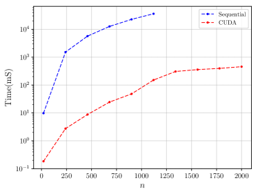
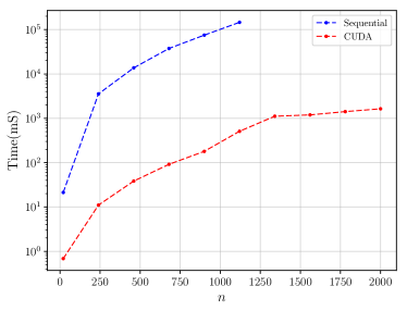
Figure 2: Timing results (in milliseconds) for sequential versus GPU-parallel computation of the forward construction (left) and gradient computation (right) with respect to orthogonal matrices whose size is on the $x$-axes. See text for discussion.

This section will present numerical results illustrating the viability of the proposed parallelizations. Prior to turning to the details, a few remarks are in order. First, we emphasize that while we have opted for a GPU-centered implementation, the main objective of this work is not to advocate a particular computing paradigm but rather to generically expose the inherent parallelizability of forward and backpropagation under angle-parametrized orthogonal matrices. GPUs are appealing due to their suitability to processing large numbers of relatively independent operations such as those present in our round-robin block matrix updates, but in principle our construction can be leveraged in any parallel computing context, e.g. multi-core CPUs, etc.

Second, it is not within the scope of this paper to exhaustively run the gamut of low-level optimization techniques to tease out the best possible performance; though clearly essential for practical adoption of the algorithm at scale, this will be left to later work. Our current proof-of-concept aim is more modest: we will compare the times taken by a sequential but reasonably efficient single-threaded CPU-centered implementation against a GPU variant instantiating the ideas in this paper. The experiments serve mostly as preliminary evidence that the promised parallel speedups appear to be real and not hindered by some unforeseen roadblock.

Both algorithms were implemented as extensions to the PyTorch Library [15]. The CPU version was written in C++, striving for efficiency by leveraging optimized tensor operations implemented in PyTorch’s ATen library when possible, and needless to say, by exploiting the sparsity structure of Givens rotations (i.e. a Givens matrix only acted on the relevant pair of rows of the operand and was most certainly not implemented as multiplication by a full $n\times n$ matrix). The GPU variant implemented the parallel operations with customized CUDA kernels (except for the backward step’s reduction, which used ATen’s summation function) and were called from sequential C++ code iterating over the $n-1$ blocks partitioning the round-robin sequence.

The CPU code was run on an Intel Xeon E5-2690 processor while the GPU runs used an Nvidia Tesla K80, hardly a state-of-the-art device at the time of writing; our aim was to measure the average time (in milliseconds) taken by each device over 50 runs of the forward and backward algorithms as a function of matrix dimension $n$. Due to the excessive time consumed by the backward stage, the sequential method only considered matrices up to size $n=1120$ while those on the GPU were allowed to be as large as $n=2000$. The timing for the GPU did not consider the latency of uploading parameters ${\boldsymbol{\theta}}$ onto the device, which should only occur once in a training context.

Results of the computations are shown in Figure 2 with the forward and backward times appearing in the left and right plots respectively, where we see that for our most likely suboptimized CUDA implementation, the speedups for both stages using the parallelizations described in this paper measure in the hundreds, strongly suggesting that a serious undertaking to engineer the code is in order, and may have positive impact on the efficiency of training RNNs and broad classes of generative models used in machine learning today.

Appendix A Adaptations to $\textrm{U}(n)$

Extension of this paper’s parallelization to the group of unitary matrices $\textrm{U}(n)$ is in principle straightforward; extra costs arise due to the need to handle the complex phase parameters but the overall complexity is essentially unchanged. In this appendix, we describe the extended parametrization involving complex phase factors(e.g. [3]), present the constructive algorithm, and describe computation of the derivatives within a block with respect to both the rotation and the phase angle parameters.

Given a coordinate pair sequence $E$, an elementary rotation associated with pair $e=(i,j)$ with $i<j$ is ${\boldsymbol{G}}^{e}(\theta_{e},\phi_{e})$, where

$$G^{e}_{ii} =G^{e}_{jj}=e^{\iota\phi_{ij}}\cos\theta_{ij}$$

$$G^{e}_{ij} =-\sin\theta_{ij}$$

$$G^{e}_{ji} =e^{\iota\phi_{ij}}\sin\theta_{ij}$$

$$G^{e}_{ll} =1\text{\quad if }l\neq i,l\neq j$$ (18)

and zero everywhere else; the phase parameters ${\boldsymbol{\phi}}=(\phi_{e_{1}},\ldots,\phi_{e_{\mathcal{N}}})$ now contribute complex phase factors $\{e^{\iota\phi_{e}}\}$ to the rotations. It should be clear that for given round-robin $E$ and parameters ${\boldsymbol{\theta}},{\boldsymbol{\phi}}$, the structure of the parallel forward construction of ${\boldsymbol{U}}$ as defined in Equation 2 is unaltered; for completeness, it is presented in Algorithm 4.

Algorithm 4 Parallel Forward ${\boldsymbol{U}}\in\textrm{U}(n)$

Input:

      Block sequence $B=(b_{1},\ldots,b_{n-1})$ such that $E$ is round-robin

      Parametrizing angles ${\boldsymbol{\theta}}=(\theta_{e_{1}},\ldots,\theta_{e_{\mathcal{N}}})$

      Parametrizing phase angles ${\boldsymbol{\phi}}=(\phi_{e_{1}},\ldots,\phi_{e_{\mathcal{N}}})$

Output:

      ${\boldsymbol{U}}({\boldsymbol{\theta}})$

${\boldsymbol{U}}\leftarrow{\boldsymbol{I}}_{n}$

for $b\in\textrm{reversed}(B)$ do

     for $e\in b$ do $\triangleright$ This block is fully parallel

         $(i,j)\leftarrow e$

         ${\boldsymbol{r}}_{i}\leftarrow e^{\iota\phi_{ij}}\cos\theta_{ij}{\boldsymbol{U}}_{i:}-\sin\theta_{ij}{\boldsymbol{U}}_{j:}$

         ${\boldsymbol{r}}_{j}\leftarrow e^{\iota\phi_{ij}}\sin\theta_{ij}{\boldsymbol{U}}_{i:}+\cos\theta_{ij}{\boldsymbol{U}}_{j:}$

         ${\boldsymbol{U}}_{i:}\leftarrow{\boldsymbol{r}}_{i}$

         ${\boldsymbol{U}}_{j:}\leftarrow{\boldsymbol{r}}_{j}$

     end for

     Synchronize parallel operations

end for

Extending the backpropagation computation takes a bit more work. The matrix

$$\frac{\partial{\boldsymbol{G}}^{e}}{\partial\theta_{e}}$$

consists of 4 nonzero elements

$$\Bigg{[}\frac{\partial{\boldsymbol{G}}^{e}}{\partial\theta_{e}}\Bigg{]}_{ii}= -e^{\iota\phi_{e}}\sin\theta_{e} \Bigg{[}\frac{\partial{\boldsymbol{G}}^{e}}{\partial\theta_{e}}\Bigg{]}_{jj}= -\sin\theta_{e}$$

$$\Bigg{[}\frac{\partial{\boldsymbol{G}}^{e}}{\partial\theta_{e}}\Bigg{]}_{ij}= -\cos\theta_{e} \Bigg{[}\frac{\partial{\boldsymbol{G}}^{e}}{\partial\theta_{e}}\Bigg{]}_{ji}= e^{\iota\phi_{e}}\cos\theta_{e}$$ (19)

while

$$\frac{\partial{\boldsymbol{G}}^{e}}{\partial\phi_{e}}$$

possesses two nonzero elements

$$\Bigg{[}\frac{\partial{\boldsymbol{G}}^{e}}{\partial\phi_{e}}\Bigg{]}_{ii}= \iota e^{\iota\phi_{e}}\cos\theta_{e} \Bigg{[}\frac{\partial{\boldsymbol{G}}^{e}}{\partial\phi_{e}}\Bigg{]}_{ji}= \iota e^{\iota\phi_{e}}\sin\theta_{e}$$ (20)

For block $b_{k}$ and $\tilde{e}\in b_{k}$, commutativity implies that

$$\frac{\partial{\boldsymbol{G}}^{b_{k}}}{\partial\theta_{\tilde{e}}}=\frac{\partial{\boldsymbol{G}}^{\tilde{e}}}{\partial\theta_{\tilde{e}}}{\boldsymbol{G}}^{\tilde{e}}{}^{\dagger}{\boldsymbol{G}}^{b_{k}}$$

$$\frac{\partial{\boldsymbol{G}}^{b_{k}}}{\partial\phi_{\tilde{e}}}=\frac{\partial{\boldsymbol{G}}^{\tilde{e}}}{\partial\phi_{\tilde{e}}}{\boldsymbol{G}}^{\tilde{e}}{}^{\dagger}{\boldsymbol{G}}^{b_{k}}$$ (21)

where $\dagger$ denotes the adjoint (conjugate/transpose) operation. Define

$${\boldsymbol{Q}}_{e}\triangleq\frac{\partial{\boldsymbol{G}}^{e}}{\partial\theta_{e}}{\boldsymbol{G}}^{e}{}^{\dagger}$$

$${\boldsymbol{P}}_{e}\triangleq\frac{\partial{\boldsymbol{G}}^{e}}{\partial\phi_{e}}{\boldsymbol{G}}^{e}{}^{\dagger}$$ (22)

Just as for the real case, the entries of ${\boldsymbol{Q}}_{e}$ are only nonzero in two locations, namely

$$\Big{[}{\boldsymbol{Q}}_{e}\Big{]}_{ij} =-1$$

$$\Big{[}{\boldsymbol{Q}}_{e}\Big{]}_{ji} =1$$ (23)

while ${\boldsymbol{P}}_{e}$ has four (purely imaginary) nonzero entries:

$$\Big{[}{\boldsymbol{P}}_{e}\Big{]}_{ii} =\iota\cos^{2}\theta_{e}$$

$$\Big{[}{\boldsymbol{P}}_{e}\Big{]}_{jj} =\iota\sin^{2}\theta_{e}$$

$$\Big{[}{\boldsymbol{P}}_{e}\Big{]}_{ij} =\Big{[}{\boldsymbol{P}}_{e}\Big{]}_{ji}=\iota\sin\theta_{e}\cos\theta_{e}$$ (24)

At step $k$, again let ${\boldsymbol{U}}^{\textrm{fwd}}={\boldsymbol{U}}^{1:k-1}$ and ${\boldsymbol{U}}^{\textrm{bck}}={\boldsymbol{U}}^{k:n-1}$, with

$${\boldsymbol{U}}^{\textrm{fwd}}=[{\boldsymbol{u}}_{1}{\boldsymbol{u}}_{2}\ldots{\boldsymbol{u}}_{n}]$$

and

$${\boldsymbol{U}}^{\textrm{bck}}=\begin{bmatrix}{\boldsymbol{v}}^{\dagger}_{1}\\ {\boldsymbol{v}}^{\dagger}_{2}\\ \vdots\\ {\boldsymbol{v}}^{\dagger}_{n}\end{bmatrix}$$

Turning back to obtaining

$$\frac{\partial{\boldsymbol{U}}}{\partial\theta_{e}}= {\boldsymbol{U}}^{\textrm{fwd}}{\boldsymbol{Q}}_{e}{\boldsymbol{U}}^{\textrm{bck}}$$

$$\frac{\partial{\boldsymbol{U}}}{\partial\phi_{e}}= {\boldsymbol{U}}^{\textrm{fwd}}{\boldsymbol{P}}_{e}{\boldsymbol{U}}^{\textrm{bck}}$$ (25)

the properties of ${\boldsymbol{Q}}_{e}$ and ${\boldsymbol{P}}_{e}$ imply that for $e\in b_{k}$

$$\frac{\partial{\boldsymbol{U}}}{\partial\theta_{e}}= {\boldsymbol{u}}_{j}{\boldsymbol{v}}_{i}^{\dagger}-{\boldsymbol{u}}_{i}{\boldsymbol{v}}_{j}^{\dagger}$$

$$\frac{\partial{\boldsymbol{U}}}{\partial\phi_{e}}= \iota\cos\theta_{e}\big{(}\cos\theta_{e}{\boldsymbol{u}}_{i}+\sin\theta_{e}{\boldsymbol{u}}_{j}\big{)}{\boldsymbol{v}}_{i}^{\dagger}+\iota\sin\theta_{e}\big{(}\cos\theta_{e}{\boldsymbol{u}}_{i}+\sin\theta_{e}{\boldsymbol{u}}_{j}\big{)}{\boldsymbol{v}}_{j}^{\dagger}$$

$$= \iota\big{(}\cos\theta_{e}{\boldsymbol{u}}_{i}+\sin\theta_{e}{\boldsymbol{u}}_{j}\big{)}\big{(}\cos\theta_{e}{\boldsymbol{v}}_{i}+\sin\theta_{e}{\boldsymbol{v}}_{j}\big{)}^{\dagger}$$ (26)

Thus, just as for the real case the derivative matrices with respect to $\{\theta_{e}\}$ are of rank 2, while those with respect to the phase angles $\{\phi_{e}\}$ have unity rank; within a block, disjoint pairs of $({\boldsymbol{u}}_{i},{\boldsymbol{u}}_{j})$ and $({\boldsymbol{v}}_{i},{\boldsymbol{v}}_{j})$ are involved in the computations of both derivative types.

Completion of the block-parallel gradient computation can then follow an analogous path to that described in Section 4.2, albeit more tediously.

References

• [1] Arjovsky, M., Shah, A., and Bengio, Y. Unitary evolution recurrent neural networks. In International Conference on Machine Learning (2016), PMLR, pp.ย 1120โ€“1128.
• [2] Baranyai, Z. On the factorization of the complete uniform hypergraphs. Infinite and finite sets (1974).
• [3] Clements, W.ย R., Humphreys, P.ย C., Metcalf, B.ย J., Kolthammer, W.ย S., and Walmsley, I.ย A. Optimal design for universal multiport interferometers. Optica 3, 12 (2016), 1460โ€“1465.
• [4] Harandi, M., and Fernando, B. Generalized backpropagation, ร‰tude de cas: Orthogonality. arXiv preprint arXiv:1611.05927 (2016).
• [5] Harris, M., etย al. Optimizing parallel reduction in CUDA. Nvidia developer technology 2, 4 (2007), 1โ€“39.
• [6] Huang, L., Liu, X., Lang, B., Yu, A., Wang, Y., and Li, B. Orthogonal weight normalization: Solution to optimization over multiple dependent Stiefel manifolds in deep neural networks. In Proceedings of the AAAI Conference on Artificial Intelligence (2018), vol.ย 32.
• [7] Jing, L., Shen, Y., Dubcek, T., Peurifoy, J., Skirlo, S., LeCun, Y., Tegmark, M., and Soljaฤiฤ‡, M. Tunable efficient unitary neural networks (EUNN) and their application to RNNs. In International Conference on Machine Learning (2017), PMLR, pp.ย 1733โ€“1741.
• [8] Kirkman, T.ย P. On a problem in combinations. Cambridge and Dublin Mathematical Journal 2 (1847), 191โ€“204.
• [9] Lezcano-Casado, M., and Martฤฑnez-Rubio, D. Cheap orthogonal constraints in neural networks: A simple parametrization of the orthogonal and unitary group. In International Conference on Machine Learning (2019), PMLR, pp.ย 3794โ€“3803.
• [10] Mathieu, M., and LeCun, Y. Fast approximation of rotations and Hessian matrices. arXiv preprint arXiv:1404.7195 (2014).
• [11] NVIDIA, Vingelmann, P., and Fitzek, F.ย H. CUDA, release: 10.2.89, 2020.
• [12] Nvidia Corporation. cuBLAS. https://developer.nvidia.com/cublas. Accessed: 2021-03-11.
• [13] Ozay, M., and Okatani, T. Optimization on submanifolds of convolution kernels in CNNs. arXiv preprint arXiv:1610.07008 (2016).
• [14] Papamakarios, G., Nalisnick, E., Rezende, D.ย J., Mohamed, S., and Lakshminarayanan, B. Normalizing flows for probabilistic modeling and inference. arXiv preprint arXiv:1912.02762 (2019).
• [15] Paszke, A., Gross, S., Massa, F., Lerer, A., Bradbury, J., Chanan, G., Killeen, T., Lin, Z., Gimelshein, N., Antiga, L., etย al. PyTorch: An imperative style, high-performance deep learning library. arXiv preprint arXiv:1912.01703 (2019).
• [16] Reck, M., Zeilinger, A., Bernstein, H.ย J., and Bertani, P. Experimental realization of any discrete unitary operator. Physical review letters 73, 1 (1994), 58.
• [17] Rezende, D., and Mohamed, S. Variational inference with normalizing flows. In International Conference on Machine Learning (2015), PMLR, pp.ย 1530โ€“1538.
• [18] Wisdom, S., Powers, T., Hershey, J.ย R., Roux, J.ย L., and Atlas, L. Full-capacity unitary recurrent neural networks. arXiv preprint arXiv:1611.00035 (2016).