Analysis and classification of main risk factors causing stroke in Shanxi Province

Abstract

Background: In China, stroke is the first leading cause of death in recent years. It is a major cause of long-term physical and cognitive impairment, which bring great pressure on National Public Health System. Evaluation of the risk of getting stroke is important for the prevention and treatment of stroke in China.

Methods: A data set with 2000 hospitalized stroke patients in 2018 and 27583 residents during the year 2017 to 2020 is analyzed in this study. Due to data incompleteness, inconsistency and non-structured formats, missing values in the raw data are filled with -1 as an abnormal class. With the cleaned features, three models on risk levels of getting stroke are built by using machine learning methods. The importance of “8+2” factors from China National Stroke Prevention Project (CSPP) is evaluated via decision tree and random forest models. Except “8+2” factors the importance of features and SHAP values for lifestyle information, demographic information and medical measurement are evaluated and ranked via random forest model. Furthermore, a logistic regression model is applied to evaluate the probability of getting stroke for different risk levels.

Results: The risk of getting stroke for the 27583 residents is categorized and labeled with the CSPP’s taxonomy: Low risk(11739 residents), Medium risk(7630 residents) and High risk(8214 residents). Among all “8+2” factors for the risk level of getting stroke, the decision tree model shows that top three features are Hypertension (importance: $0.4995$), Physical Inactivity (importance: $0.08486$) and Diabetes Mellitus (importance: $0.07889$), and the random forest model shows that top three features are Hypertension (importance: $0.3966$), Hyperlipidemia (importance: $0.1229$) and Physical Inactivity (importance: $0.1146$). Except “8+2” factors the importance of features for lifestyle information, demographic information and medical measurement is evaluated via random forest model. It shows that top five features are Systolic blood pressure (importance: $0.3670$), Diastolic blood pressure (importance: $0.1541$), physical inactivity (importance: $0.0904$), Body Mass Index(BMI) (importance: $0.0721$) and Fasting Blood Glucose(FBG) (importance: $0.0531$). SHAP values show that Diastolic blood pressure, physical inactivity, Systolic blood pressure, BMI, smoking, FBG, and Triglyceride(TG) are positively correlated to the risk of getting stroke. High-density lipoprotein (HDL) is negatively correlated to the risk of getting stroke. Combining with the data of 2000 hospitalized stroke patients, the logistic regression model shows that the average probabilities of getting stroke are $7.20\%$ (with $95\%$ CI: $(6.65\%,7.74\%)$) for the low-risk level patients, $19.02\%$ (with $95\%$ CI: $(18.08\%,19.96\%)$) for the medium-risk level patients and $83.89\%$ (with $95\%$ CI: $(82.93\%,84.86\%)$) for the high-risk level patients.

Conclusion: Based on the census data in both communities and hospitals from Shanxi Province, we investigate different risk factors of getting stroke and their ranking with interpretable machine learning models. The results show that Hypertension (Systolic blood pressure, Diastolic blood pressure), Physical Inactivity (Lack of sports), and Overweight (BMI) are ranked as the top three high risk factors of getting stroke in Shanxi province. The probability of getting stroke for a person can also be predicted via our machine learning model.

1 Introduction

Stroke, an acute cerebrovascular disease, is caused by brain tissue damage due to abnormal blood supply to the brain with cerebrovascular blockage. It includes hemorrhagic stroke and ischemic stroke. According to the Global Burden of Disease, Injuries and Risk Factor Study and other researches [1, 2, 3], stroke is the third leading cause of death in the world and the first in China. Recent studies from National Epidemiological Survey of Stroke in China(NESS-China) [4] show the prevalence of stroke in China during 2012-2013:

Region	Prevalence (Per 100000)	Incidence (per 100000)	Mortality (per 100000)
Central China	1549.5	326.1	153.7
Northeast China	1450.3	365.2	158.5
South China	624.5	154.6	65

Table 1: Prevalence of Stroke in China

Investigation into risk factors of getting stroke is essentially important for the prevention of stroke. Research shows that risk factors can be divided into two categories: reversible factors and irreversible factors.

Reversible factors mainly refer to unhealthy lifestyles such as smoking, excessive alcohol consumption and physical inactivity; while irreversible factors mainly refer to chronic diseases such as hypertension, diabetes, and hyperlipidemia. A number of researches on stroke risk analysis have been done for the European and American populations [5, 6]. However, they can not be directly applied to the Chinese population due to racial difference.

In China, stroke-related research is mostly carried out on risk prediction models with pathogenic factors. The most widely used one is the 10-year risk prediction model using cardiovascular and cerebrovascular diseases to give probability of stroke and coronary heart disease incidence. The CHINA-PAR project (Prediction for ASCVD Risk in China) led by Gu Dongfeng’s team [7] proposed a revised model which considered not only the 10-year risk but also a lifetime-risk assessment. By analyzing data on the incidence of stroke in 32 of 34 provincial regions of China, Xu et al. [8] concluded that there is a stroke belt in north and west China.

In recent years, some machine learning methods have been applied to the stroke prediction. In 2010, a combination of Support Vector Machine and Cox Proportional Hazard Model was proposed by Khosla et al. [9]. Benjamin [10] implemented an interpretable method using Decision List with Bayesian Analysis to quantify the probability of stroke. Chi-Chun Lee’s team [11, 12] compared multiple methods including Deep Neural Network in stroke prediction with Electronic Health Records (EHR). In their research, they focus on the patient’s 3 year stroke rate and 8 year stroke rate. However, few of these studies modeled the early screening and prevention of stroke.

Evaluation of the risk of getting stroke is important for prevention and treatment of stroke in China. The China National Stroke Prevention Project (CSPP) proposed “8 + 2” main risk factors in identifying Chinese residents’ risk level of getting stroke [13, 14, 15]:

• Hypertension

• Diabetes mellitus

• Heart disease(includes atrial fibrillation and valvular heart disease)

• Hyperlipidemia

• Family history of stroke

• Overweight

• Smoking

• Physical inactivity

• The history of stroke

• The history of Transient Ischemic Attack (TIA)

With the above proposed “8+2” main risk factors, the risk level of getting stroke can be classified into:

• High risk: having at least three factors from factor 1 to 8; or one of a and b;

• Medium risk: having less than three risk factors from factor 1 to 8 with at least one being factor 1, 2 or 3;

• Low risk: having less than three risk factors from factor 4 to 8.

However, the ranking of the risk factors may present differently in different provinces. Based on the census data in both communities and hospitals from Shanxi Province, in this paper, we investigates different stroke risk factors and their ranking. It shows that hypertension, physical inactivity (lack of sports), and overweight are ranked as the top three high stroke risk factors in Shanxi. The probability of getting a stroke is also estimated through our interpretable machine learning methods. The study provides theoretical support for stroke prevention and control in Shanxi Province.

2 Materials and Methods

2.1 Dataset and Preprocessing

Our data is composed by two survey datasets from 2017 to 2020:

• Census in hospital: 2000 hospitalized stroke patients in 2018;

• Census in community: 27583 residents during the year 2017 to 2020. This dataset is categorized and labeled with the CSPP’s taxonomy: Low risk (11739), Medium risk (7630) and High risk (8214).

Each record in both datasets contains 177 features, not only providing information on the “8+2” risk factors but also patients’ other information:

Feature Name	Example
Demographic information	Sex, Ethnicity, etc.
Lifestyle information	Smoking, Alcohol consumption, etc.
Medical measurement	Blood pressure, fasting blood glucose, etc.
Surgery information	history of surgery (PCI, CABG, CEA, CAS)
Chronic diseases information	diagnosis times, what kinds of treatment

Data cleansing is a preparation process in data analysis by removing or correcting data that is corrupt or inaccurate. The raw data in the above datasets needs to be cleaned due to data incompletion, inconsistence and non-structured formats which may lead to a failure of feature engineering. In this paper, missing values of a feature are filled with -1 as an abnormal class. If there is over $60\%$ missing inside the column, we will delete it since the data from the column cannot provide much information. Inconsistent values are found and corrected with prior medical knowledge. For instance, diastolic blood pressure should be lower than systolic blood pressure.

After the data cleansing, there are total 23289 records (low: 9718, mid: 6742, high: 5610) with 32 features in remains, shown in Table 2.

Class	Feature Name	Data Type
Lifestyle Information	Favor	Categorical
Lifestyle Information	Alcohol	Categorical
Lifestyle Information	Frequency of Vegetables	Categorical
Lifestyle Information	Frequency of Fruits	Categorical
Lifestyle Information	Meat and Vegetables	Categorical
Lifestyle Information	Medical Payment Method	Categorical
Demographic Information	Sex	Categorical
Demographic Information	Age	Numerical
Demographic Information	BMI	Numerical
Demographic Information	Retire	Categorical
Demographic Information	Height	Numerical
Demographic Information	Weight	Numerical
Demographic Information	Ethnicity	Categorical
Demographic Information	Occupation	Categorical
Demographic Information	Marital Status	Categorical
Demographic Information	Education Level	Categorical
Medical Measurement	TC	Numerical
Medical Measurement	TG	Numerical
Medical Measurement	HDL	Numerical
Medical Measurement	LDL	Numerical
Medical Measurement	HCY	Numerical
Medical Measurement	FBG	Numerical
Medical Measurement	Pulse	Numerical
Medical Measurement	Systolic blood pressure	Numerical
Medical Measurement	Diastolic blood pressure	Numerical
“8+2” Factor and Lifestyle Information	Smoking	Categorical
“8+2” Factor and Lifestyle Information	Physical Inactivity	Categorical
“8+2” Factor and Medical Information	Heart Disease	Categorical
“8+2” Factor and Medical Information	Hypertension	Categorical
“8+2” Factor and Medical Information	Hyperlipidemia	Categorical
“8+2” Factor and Medical Information	History of Stroke	Categorical
“8+2” Factor and Medical Information	Diabetes Melltius	Categorical
“8+2” Factor and Medical Information	Family history of Stroke	Categorical
“8+2” Factor and Medical Information	History of Transient Ischemic Attack	Categorical

Table 2: Remaining features after Data Cleansing

2.2 Models

Decision-Tree is a classic non-parametric machine learning algorithm. A tree is created through learning decision rules inferred from data features. Starting from the top root node, data are split into different internal nodes according to certain cutoff values in features, and then finally arrive the terminal leaf nodes which give the final classification result. ID3 [16] and CART [17] are classic Decision-Tree algorithms which employ Information Gain and Gini Impurity from Entropy Theory [18] as measurements in making best splitting rules.

Random-Forest is a machine learning algorithm proposed by Leo Breiman[19] in 2001. Instead of using one decision tree which is nonunique and may exhibits high variance, random forest generates a number of individual decision trees operating as a committee. Bootstrapping technique is used to train the individual decision trees in parallel on different sub datasets and features with random sampling with replacement. The final decision of classification is aggregated by voting and averaging. With the wisdom of crowds, random forest can easily overcome overfitting problem and reduce model bias caused by data imbalance, and thus shows good generalization.

Logistic model is a generalized linear model which is widely used in data mining. It assumes that the dependent variable $y$ follows a Bernoulli distribution and introduces non-linear factors through the Sigmoid function:

$$y=\frac{1}{1+e^{-z}},$$

where $z=\beta_{0}+\beta_{1}x_{1}+\dots+\beta_{n}x_{n}$ and $n$ is the number of features.

Assumes that $y$ represents a binary outcome $\{0,1\}$, and $X$ is an array of their features and $\beta_{i}$ is the coefficient of feature $x_{i}$ [20]. The coefficient in logistic regression is called log odds and used in logistic regression equation for the prediction of the dependent variable $y$ from the independent variable $X$, let $p=P(y=1)$:

$$log\left(\frac{p}{1-p}\right)=\beta_{0}+\beta_{1}x_{1}+\dots+\beta_{n}x_{n}\Rightarrow p=\frac{exp(\beta_{0}+\beta_{1}x_{1}+\dots+\beta_{n}x_{n})}{1+exp(\beta_{0}+\beta_{1}x_{1}+\dots+\beta_{n}x_{n})}$$

In practice, Logistics Regression can be used in multiple aspects, for instance, advertising, disease diagnosis as it can provide the possibility of a user buying a certain product and the possibility of a certain patient suffering from a certain disease. In our case, we want to use the “8+2” risk factors and resident’s lifestyle factors as input and give out the probability of stroke incidence, which can provide a forward-looking prediction.

2.3 Model’s Interpretation

The model’s interpretability and explanations are crucial for the medical data analysis: the medical diagnosis system must be transparent, understandable, and explainable. Therefore, the doctor and the patient can know how the model makes decisions, which features are important, and how the features affect the model’s result [21, 22]. In this section, we mainly introduce the feature importance, permutation importance and SHAP value which can help interpret the model.

Feature importance, also called as Gini importance or Mean Decrease Impurity (MDI)[19, 23, 24], is the average of node impurity decrease of each variable and weighted by the probability of the sample reaching to that node. For Random-Forest model, assumes that the response is $Y$ and to calculate the average variable importance of feature $X_{i}$ with $N$ trees:

$$Imp(X_{i})=\frac{1}{N}\sum_{T=1}^{N}\sum_{j\in T:v(s_{j})=X_{m}}p(j)\Delta i(s_{j},j)$$

Where $p(j)\Delta i(s_{j},j)$ is the weighted impurity decreases for feature $X_{i}$ in all nodes $j$, $p(j)$ is the probability of the sample reading to node ($p(j)=\frac{N_{j}}{N}=\frac{\text{the amount of samples reaching the node $j$}}{\text{total amount of samples}}$) and $i(s_{j},j)$ is the impurity measure at node $j$ with split $s_{j}$. $v(s_{j})$ is the variable used in the split $s_{j}$(split $s_{j}$ means the split at node $j$. Hence, $v(s_{j})=X_{m}$ means at node $j$, the splitting identifier is variable $X_{m}$).

For the Decision-Tree model, it only contains one tree, that is, $N=1$, and its feature importance can be rewritten as:

$$Imp(X_{i})=\sum_{v(s_{j})=X_{m}}p(j)\Delta i(s_{j},j)$$

Permutation Importance [19, 25, 26, 24], is used in answering how a certain feature influence the overall prediction, as it evaluates the changes of model prediction’s accuracy by permuting the feature’s values. If let $s$ represent the model accuracy with the full dataset $D$, then the permutation feature importance of $i^{th}$ feature is:

$$Per_{Imp}(i)=s-\frac{1}{K}\sum_{j=1}^{K}s_{i,j},$$

where $j$ represents the $j^{th}$ repetition in $K$ times shuffling for $i^{th}$ feature , $s_{i,j}$ as the model accuracy in modified dataset $\hat{D}_{i,j}$ with $i^{th}$ feature shuffled. With the average changed accuracy before and after shuffling can we evaluate the importance of $i^{th}$ feature.

These two importance values can show which feature is more important, however, it is unavailable for us to know whether the feature has a positive or negative effect respect to the output.

SHAP(Shapley Additive explanations) can provide not only the importance of the features but also show how much each feature contributes, either positively or negatively, to the target variable. It is a method to explain each individual prediction. This idea of SHAP value comes from the Shapley value in game theory. Shapley value tells how to fairly distribute the contributions among the features, which is the marginal contributions for each feature[27].

The goal of SHAP is to explain the prediction of an instance ${x}^{i}$ by computing the contribution of each feature to the prediction model. The formula of SHAP is an addictive feature attribution linear model, and it is shown below:

$${{\phi}_{i}}=\sum\limits_{S\subseteq F\backslash{\{{x}^{i}\}}}{\frac{|S|!(n-|S|-1)!}{n!}}\left[v(S\cup\{{x}^{i}\})-v(S)\right]$$

with $S\subseteq\{{{x}^{1}},{{x}^{2}},\cdots,{{x}^{n}}\}\backslash{{x}^{i}},F=\{{{x}^{1}},{{x}^{2}},\cdots,{{x}^{n}}\}.$

With this method, we calculate how the feature contributes to each coalition of each decision tree model and sum them up to get the total contribution of the whole prediction model. In this equation, $F\backslash{\{{x}^{i}\}}$ represents all the possible subsets without feature ${x}^{i}$, $S$ represents the sub-feature set that did not contain the result, $v(S\bigcup\{{x}^{i}\})$ represents the model output (precision, recall or accuracy, etc.) after feature ${x}^{i}$ is added to subset $S$, $v(S)$ represents the model output using subset $S$. With the multiplication for the occurrence probability for each subsets without that feature and the output different with and without that feature, the marginal contribution of each feature ${x}^{i}$ is calculated.

SHAP has three properties: local accuracy, missingness, and consistency [28]. Local accuracy means that when approximating the original model for a specific input $x$, local accuracy requires the explanation model to at least match the output of the model for the simplified input $x^{\prime}$. Missingness means that if there is a feature missing in the sample, it does not affect the output of the model. Consistency means that when the model changes and the marginal contribution of a feature increases, the corresponding Shapley value will also increase. Therefore, it is more accurate and scientific in interpreting machine learning models due to those three characteristics.

3 Result

3.1 Main Risk Factors Ranking

Due to geographic and cultural differences, the same disease may have different manifestations in different region. We hope to find the topmost influential factors in Shanxi Province. Table 3 shows the proportion of each risk factor’s Exposure rate and the Risk attribution (RA) based on our data:

Feature	Exposure rate	Risk attribution
Hypertension	0.5158	1.187
Hyperlipidemia	0.3765	0.5846
Physical Inactivity	0.3892	1.721
Overweight	0.3373	0.6844
Smoking	0.2058	1.539
Family history of stroke	0.0999	1.590
Diabetes Mellitus	0.0709	2.613
History of stroke	0.0483	NA
Heart Disease	0.0052	11.84
History of TIA	0.0023	NA

Table 3: Main Risk Factor Exposure rate and Risk attribution

To assess the ranking of main risk factors, in the first experiment, we used the dataset 2 with the “8+2” factors as feature and implemented the Decision-Tree model. Table 4 shows the classification result:

	precision	recall	f1-score	support
Low risk	0.9707	0.9950	0.9827	1999
Mid risk	0.9711	0.9411	0.9599	1313
High risk	0.9751	0.9650	0.9678	1345
accuracy			0.9721
macro avg	0.9794	0.9787	0.9789	4657
weighted avg	0.9799	0.9796	0.9795	4657

Table 4: Result of Decision Tree model

Figure 1 shows the feature importance and permutation importance based on the Decision Tree model, which shows the ranking of these main risk factors: both evaluation methods confirm that hypertension, physical inactivity, and hyperlipidemia are estimated as the top three informative features in the Decision-Tree model.

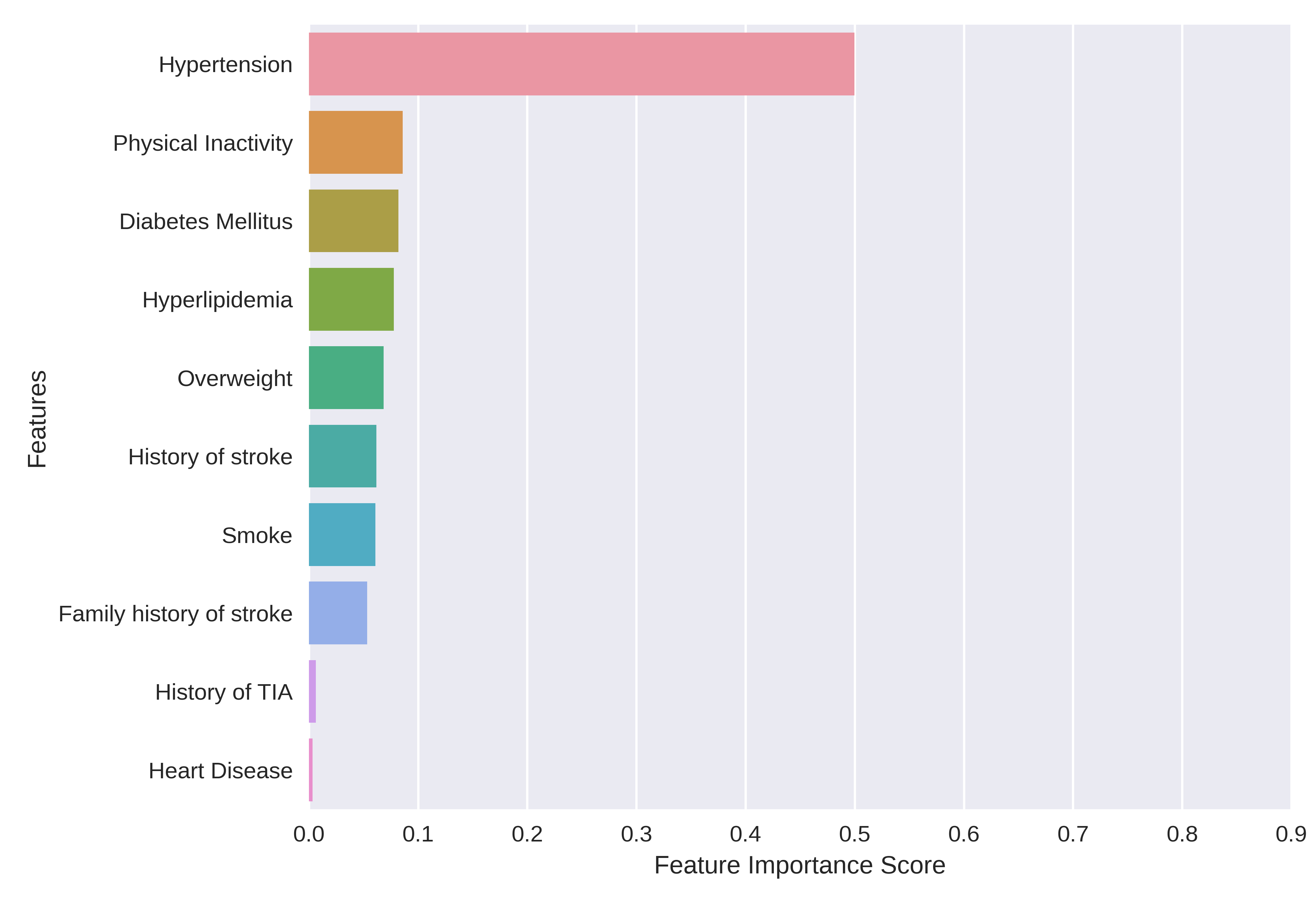
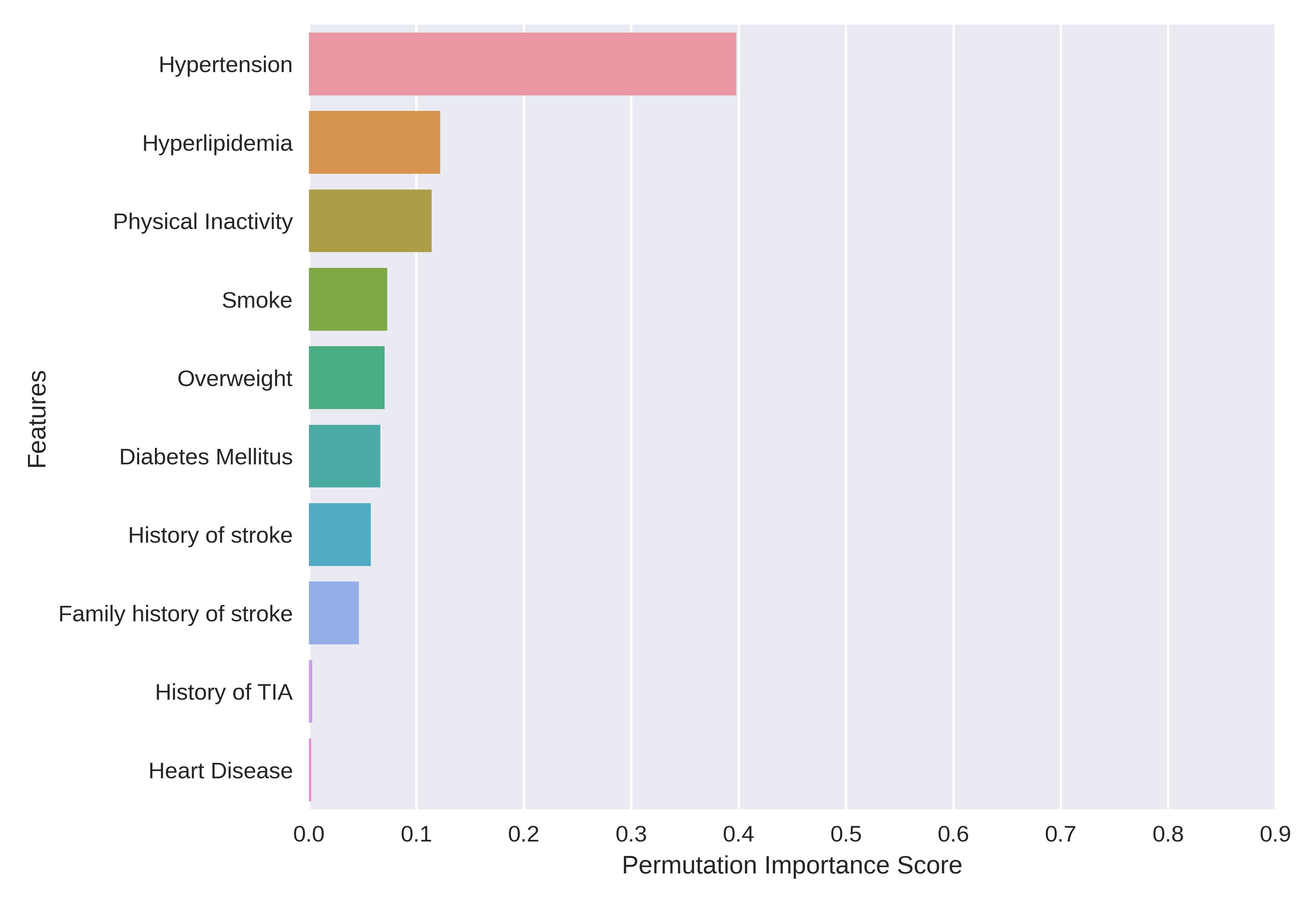
Figure 1: Feature and Permutation Importance of “8+2” Risk factor

3.2 Lifestyle and Medical Measurement Ranking

For the second experiment, we would like to identify more risk factors for Shanxi Province besides the ”8+2” risk factors by using the dataset 2 with features such as lifestyle habits and medical measurement. Table 5 shows the classification result and Figure 4 shows the feature and permutation importance:

	precision	recall	f1-score	support
Low risk	$0.8007(\pm 0.007)$	$0.9531(\pm 0.004)$	$0.8703(\pm 0.0041)$	$1962$
Mid risk	$0.8213(\pm 0.008)$	$0.7850(\pm 0.011)$	$0.7901(\pm 0.0064)$	$1367$
High risk	$0.9124(\pm 0.013)$	$0.7182(\pm 0.010)$	$0.8026(\pm 0.0076)$	$1426$
accuracy			$0.84(\pm 0.01)$
macro avg	$0.8421(\pm 0.0081)$	$0.8179(\pm 0.011)$	$0.8271(\pm 0.0034)$	$4755$
weighted avg	$0.8311(\pm 0.0095)$	$0.8400(\pm 0.010)$	$0.8344(\pm 0.0062)$	$4755$

Table 5: Result of Decision Tree model

The results shown in Figure 4 confirm that systolic blood pressure, diastolic blood pressure, physical inactivity, BMI, smoking, FBG, TG, HDL, family history of Stroke and weight are the top ten factors when we only consider the lifestyle habits, demographic information, and medical measurement. These factors are, medically, highly corresponding to the Chronic diseases [29, 30, 31].

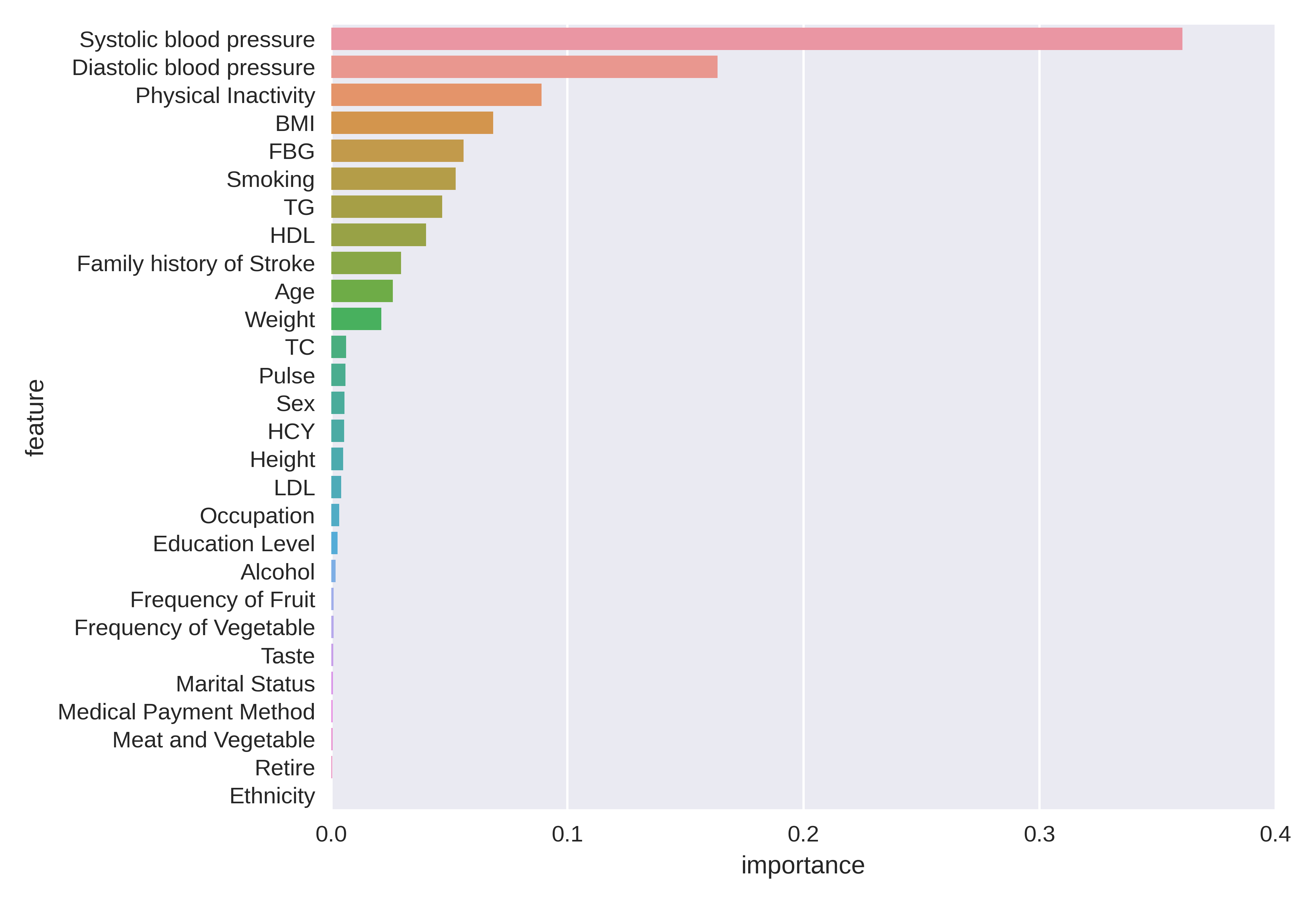
Figure 2: Feature Importance

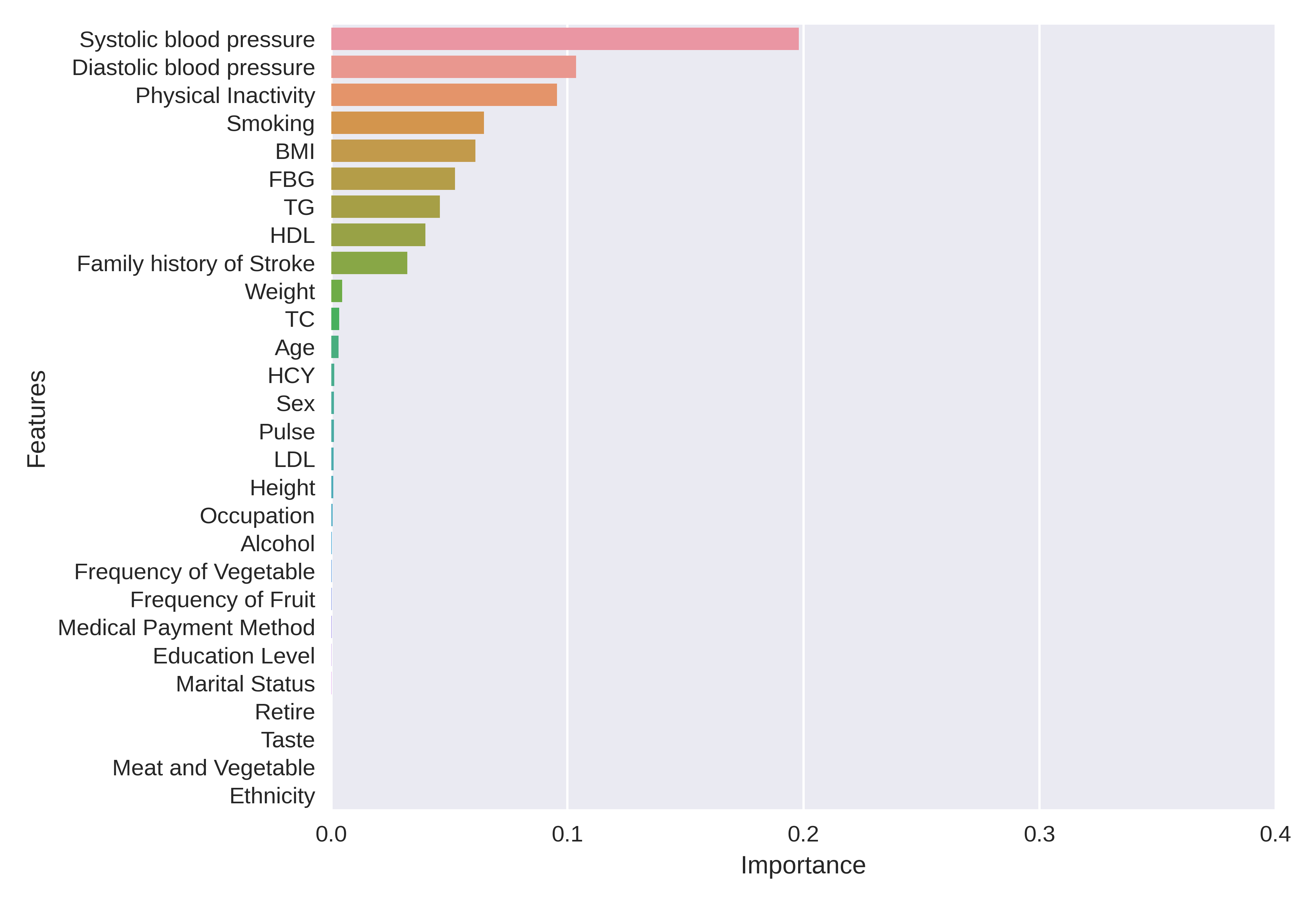
Figure 3: Permutation Importance

Figure 4: Feature and Permutation Importance of lifestyle and medical measurement factors factor

To give out the specific details on how each feature contributes to each individual, we calculate the SHAP value in the Random Forest model and use the summary-plot to show their importance. The figure of ordered mean sample SHAP value for each feature is shown in Figure 5. It shows the distribution of the contributions each factor has on the cause of stroke. The color represents the feature value (red represents high, blue represents low). The more difference for the distribution between high feature value and low feature value, the better it would be in separating patients with different risk levels. Figure 5 shows that Diastolic Blood Pressure, Physical inactivity, Systolic Blood Pressure, BMI, Smoking, FBG, and TG are positively correlated to the risk of stroke, and HDL are negatively correlated to the risk.

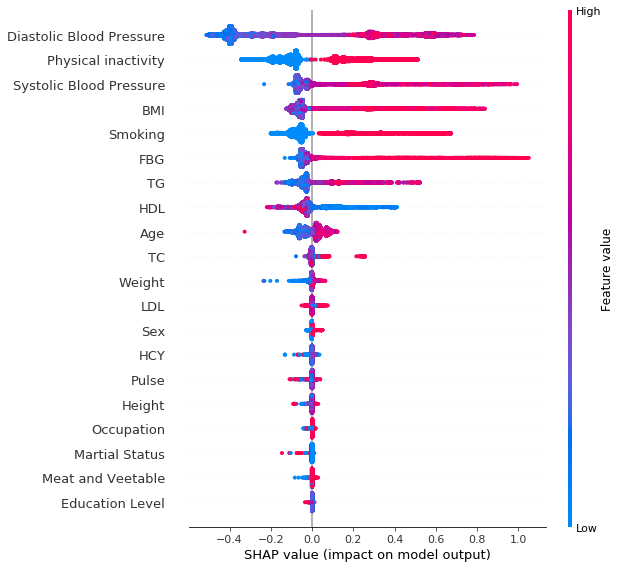
Figure 5: TreeSHAP value of top lifestyle and medical measurement factors factors

3.3 Quantitative Prediction of Stroke’s Incidence

For the third experiment, a logistic model is establish to quantify the probability of stroke incidence. To achieve this goal, we combine the dataset 1 and 2, relabel the data: the original low-risk and medium-risk are now class 0, the high-risk and stroke are class 1. The features contains lifestyle information, demographic information, and the “8+2” factors.

Logistic regression is feature-sensitive. Feature selection is done before modeling. To solve the multicollinearity problem [32], the highly relevant features are removed first. For example, we keep BMI and remove height and weight. What’s more, Variance Threshold [33] is used to remove low variance features. It is a simple method of feature selection, where deletes all the features whose variance does not meet a certain threshold. For example, most of the respondent in our survey are Han Chinese, therefore, we remove ethnicity.

The logistic model results are shown in Table 6 including the features’ coefficient, standard error, and the confidence interval. According to the coefficients, it yields that History of stroke, Physical inactivity, Hypertension, Hyperlipidemia, Smoke, Diabetes Mellitus, BMI, Family history of stroke and Heart disease are positive correlated to stroke incidence; Education level, Frequency of vegetables, and Occupation are negative correlated to stroke incidence.

y=1	coef	std err	z	$P>|z|$	95% CI [0.025, 0.975]
History of Stroke	2.6779	0.247	10.853	0.000	2.194	3.162
Physical Inactivity	1.3948	0.027	50.815	0.000	1.341	1.449
Hypertension	1.1489	0.027	41.970	0.000	1.095	1.203
Hyperlipidemia	1.0875	0.025	43.210	0.000	1.038	1.137
Smoke	1.0455	0.031	33.892	0.000	0.985	1.106
Diabetes Mellitus	0.8043	0.025	32.525	0.000	0.756	0.853
BMI	0.7897	0.026	30.635	0.000	0.739	0.840
Family history of stroke	0.7447	0.024	30.522	0.000	0.697	0.793
Heart Disease	0.4257	0.029	14.630	0.000	0.369	0.483
Frequency of Fruit	0.1507	0.026	5.817	0.000	0.100	0.202
Alcohol	0.1325	0.025	5.198	0.000	0.083	0.182
Pulse	0.1279	0.023	5.606	0.000	0.083	0.173
Sex	0.0863	0.029	2.945	0.003	0.029	0.144
Retire	0.0754	0.025	3.015	0.003	0.026	0.125
Age	0.0548	0.026	2.084	0.037	0.003	0.106
Frequency of Vegetables	-0.2262	0.025	-9.118	0.000	-0.275	-0.178
Occupation	-0.2166	0.026	-8.308	0.000	-0.268	-0.165
Education Level	-0.3640	0.027	-13.604	0.000	-0.416	-0.312
constant	-0.7868	0.068	-11.545	0.000	-0.920	-0.653

Table 6: Features’ Coefficient and Confidence Interval

The trained model is implemented on the testing set to estimate the probability of stroke incidence for each category. The results are in Table 7:

Risk Level	Average Probability of Stroke
Low	$0.0720\ (95\%CI:(0.0665,0.0774))$
Medium	$0.1902\ (95\%CI:(0.1808,0.1996))$
High	$0.8389\ (95\%CI:(0.8293,0.8486))$

Table 7: The average stroke probability for each risk level based on Logistic Model

Comparing with the qualitative ranking method, we quantify the risk factors of stroke, and convert the scoring grades into probabilities, making the prediction of stroke risk more intuitive. What’s more, our logistic model is based on the current actual circumstance to predict the incidence promptly, which is more time-sensitive.

4 Discussion

4.1 The Risk Factors in Shanxi Province

Based on the treeSHAP value, feature and permutation importance of lifestyle and medical measurement, we have found the most important factors of causing stroke:

1. Hypertension(Diastolic Blood pressure and Systolic Blood Pressure)

2. Physical Inactivity

3. Overweight (BMI)

4. Hyperlipidemia (mostly according to the HDL and TC)

5. Diabetes Mellitus (according to the FBG)

The treeSHAP dependence plot is applied to compare the contribution between two features. Figure 7 shows that Diastolic Blood Pressure ($>$ 140 mmHg) is more suitable in diagnosing the risk of patients getting a stroke than the Systolic Blood Pressure ($>$ 90 mmHg). Similarly, based on the comparison between HDL and LDL (see Figure 7), we can find that high-density lipoprotein are better in diagnosing those non-stroke patients in low high-density lipoprotein.

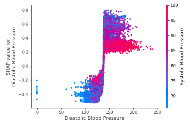
Figure 6: Dependence Plot for Systolic Blood Pressure and Diastolic Blood Pressure

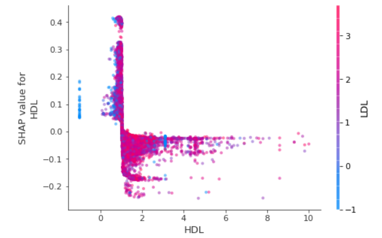
Figure 7: Dependence Plot for HDL and LDL

4.2 Feature Validity

Missing data due to the technique errors (like typos and facilities errors) is a common problem during the census analysis. To find out how might those error data in the datasets might influence, we have conducted an experiment to find out missing data in features and its influence on the final results. The Random Forest Classifier is adopted to predict the stroke risk with different proportions of a single missing feature and looped for 100 times at random locations. What’s more, to prevent the precision score didn’t change due to the strong-correlation of features, some specific feature pairs are cleaned up. The result is shown in Figure 8 :

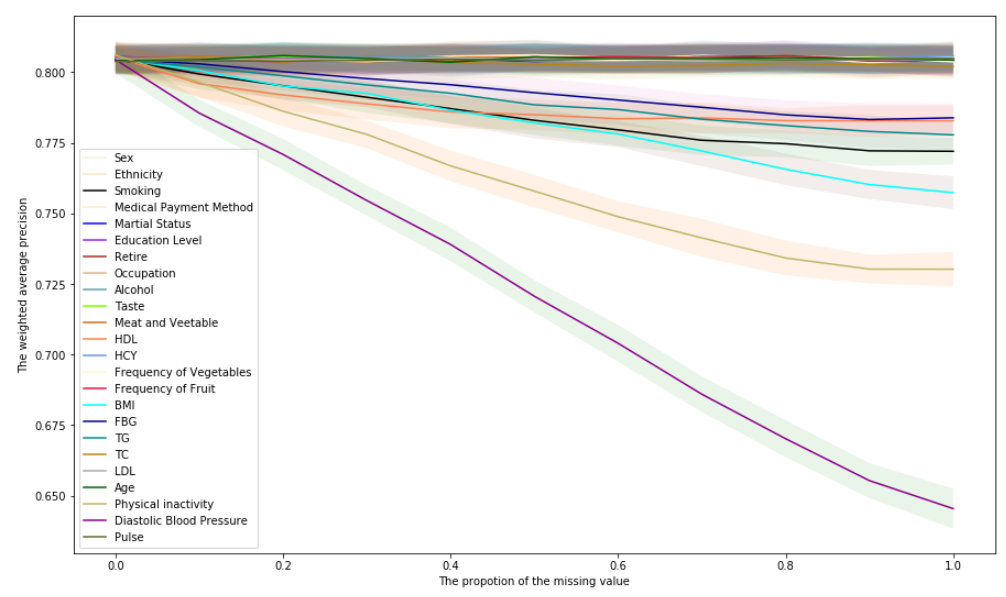
Figure 8: The relationship between the proportion of missing data in feature and the weighted precision score

In Figure 8, the curve for each feature represents how the average weight precision score of the feature has changed with the increasing proportion of the feature missing and the shadows are the 95% confidence area 100 times for each feature. Based on the result, we can see that diastolic blood pressure, physical inactivity, BMI, smoking, alcohol, HDL, and FBG are in order important factors when identifying the cause of stroke, while the other factors are not influencing the whole models. An interesting fact we have seen is that HDL seems to be a great influential factor when the proportion of HDL is small compared to most of the influenced factors.

What’s more, a Recursive Feature Elimination (RFE) process is also done to evaluate the specific amount of factors for analyzing the risk level of patients getting a stroke. The procedure of the RFE is as follows. First, the estimator is trained on the initial feature set and the importance of each feature is obtained from any specific or callable attribute. Then, the least important features are removed from the current feature set. This process is repeated recursively over the pruning set until the number of features to be selected is finally reached. Based on the Figure 9, we have found that approximate 7 features can help the Random Forest model to get a stable precision for different levels of risk. Therefore, the validity of those features is proved.

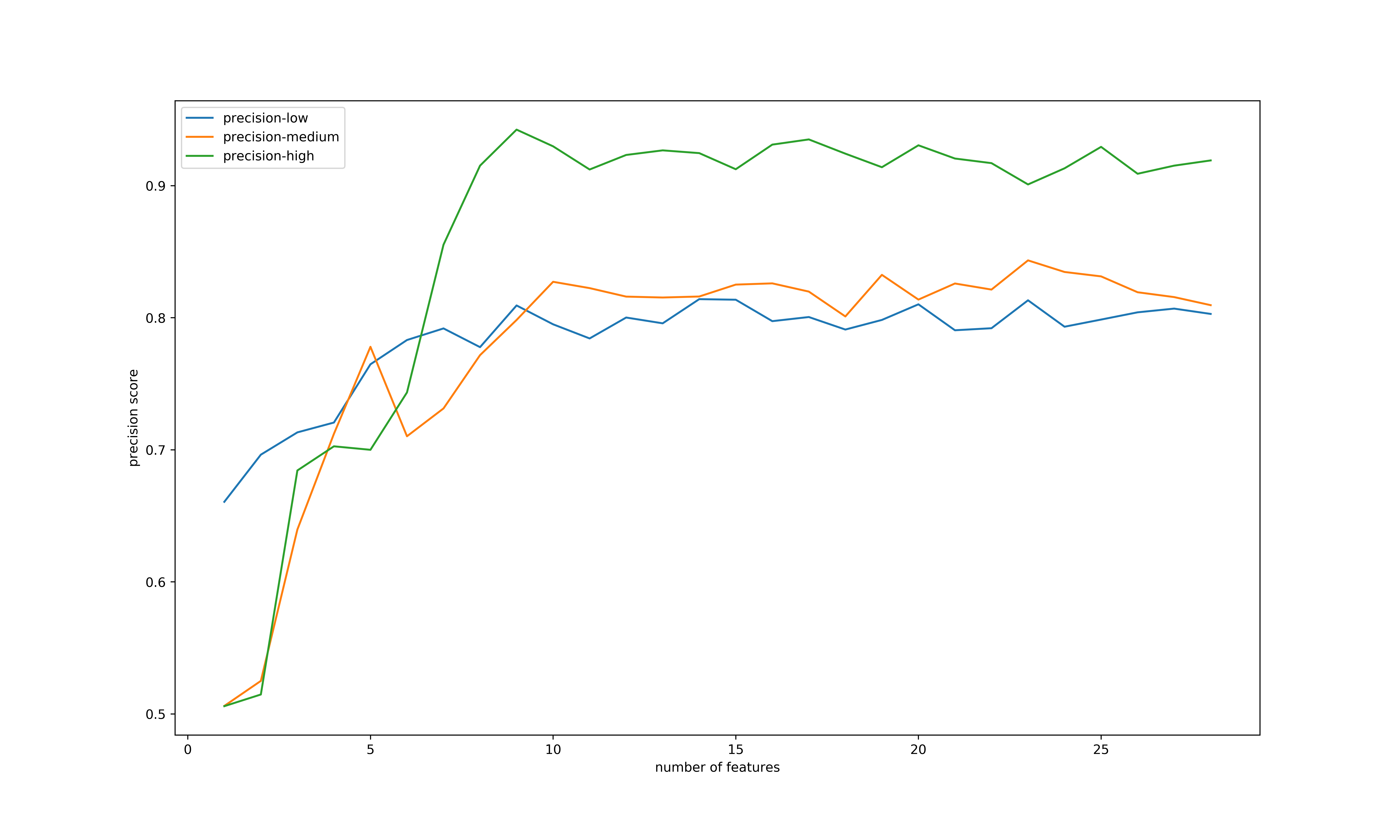
Figure 9: The relationship between the amount of features and the precision changed

References

- [1] Ming Liu, Bo Wu, Wen-Zhi Wang, Li-Ming Lee, Shi-Hong Zhang, and Ling-Zhi Kong. Stroke in china: epidemiology, prevention, and management strategies. The Lancet Neurology, 6(5):456–464, 2007.
- [2] Gregory A Roth, Degu Abate, Kalkidan Hassen Abate, Solomon M Abay, Cristiana Abbafati, Nooshin Abbasi, Hedayat Abbastabar, Foad Abd-Allah, Jemal Abdela, Ahmed Abdelalim, et al. Global, regional, and national age-sex-specific mortality for 282 causes of death in 195 countries and territories, 1980–2017: a systematic analysis for the global burden of disease study 2017. The Lancet, 392(10159):1736–1788, 2018.
- [3] Maigeng Zhou, Haidong Wang, Xinying Zeng, Peng Yin, Jun Zhu, Wanqing Chen, Xiaohong Li, Lijun Wang, Limin Wang, Yunning Liu, et al. Mortality, morbidity, and risk factors in china and its provinces, 1990–2017: a systematic analysis for the global burden of disease study 2017. The Lancet, 394(10204):1145–1158, 2019.
- [4] Wenzhi Wang, Bin Jiang, Haixin Sun, Xiaojuan Ru, Dongling Sun, Linhong Wang, Limin Wang, Yong Jiang, Yichong Li, Yilong Wang, et al. Prevalence, incidence, and mortality of stroke in china: results from a nationwide population-based survey of 480 687 adults. Circulation, 135(8):759–771, 2017.
- [5] Erkki Vartiainen, Tiina Laatikainen, Markku Peltonen, and Pekka Puska. Predicting coronary heart disease and stroke: the finrisk calculator. Global heart, 11(2):213–216, 2016.
- [6] Thomas Lumley, Richard A Kronmal, Mary Cushman, Teri A Manolio, and Steven Goldstein. A stroke prediction score in the elderly: validation and web-based application. Journal of clinical epidemiology, 55(2):129–136, 2002.
- [7] Xueli Yang, Jianxin Li, Dongsheng Hu, Jichun Chen, Ying Li, Jianfeng Huang, Xiaoqing Liu, Fangchao Liu, Jie Cao, Chong Shen, et al. Predicting the 10-year risks of atherosclerotic cardiovascular disease in chinese population: the china-par project (prediction for ascvd risk in china). Circulation, 134(19):1430–1440, 2016.
- [8] Gelin Xu, Minmin Ma, Xinfeng Liu, and Graeme J Hankey. Is there a stroke belt in china and why? Stroke, 44(7):1775–1783, 2013.
- [9] Aditya Khosla, Yu Cao, Cliff Chiung-Yu Lin, Hsu-Kuang Chiu, Junling Hu, and Honglak Lee. An integrated machine learning approach to stroke prediction. In Proceedings of the 16th ACM SIGKDD international conference on Knowledge discovery and data mining, pages 183–192, 2010.
- [10] Benjamin Letham, Cynthia Rudin, Tyler H McCormick, David Madigan, et al. Interpretable classifiers using rules and bayesian analysis: Building a better stroke prediction model. Annals of Applied Statistics, 9(3):1350–1371, 2015.
- [11] Chen-Ying Hung, Wei-Chen Chen, Po-Tsun Lai, Ching-Heng Lin, and Chi-Chun Lee. Comparing deep neural network and other machine learning algorithms for stroke prediction in a large-scale population-based electronic medical claims database. In 2017 39th Annual International Conference of the IEEE Engineering in Medicine and Biology Society (EMBC), pages 3110–3113. IEEE, 2017.
- [12] Chen-Ying Hung, Ching-Heng Lin, Tsuo-Hung Lan, Giia-Sheun Peng, and Chi-Chun Lee. Development of an intelligent decision support system for ischemic stroke risk assessment in a population-based electronic health record database. PloS one, 14(3):e0213007, 2019.
- [13] Jinghui Yu, Huajian Mao, Mei Li, Dan Ye, and Dongsheng Zhao. Csdc—a nationwide screening platform for stroke control and prevention in china. In 2016 38th Annual International Conference of the IEEE Engineering in Medicine and Biology Society (EMBC), pages 2974–2977. IEEE, 2016.
- [14] Xuemeng Li, Di Bian, Jinghui Yu, Mei Li, and Dongsheng Zhao. Using machine learning models to improve stroke risk level classification methods of china national stroke screening. BMC medical informatics and decision making, 19(1):1–7, 2019.
- [15] Bao-Hua Chao, Feng Yan, Yang Hua, Jian-Min Liu, Yi Yang, Xun-Ming Ji, Bin Peng, Guo-Guang Zhao, Yong-Jun Wang, De-Zhi Kang, et al. Stroke prevention and control system in china: Csppc-stroke program. International Journal of Stroke, 16(3):265–272, 2021.
- [16] J. Ross Quinlan. Induction of decision trees. Machine learning, 1(1):81–106, 1986.
- [17] Leo Breiman, Jerome Friedman, Charles J Stone, and Richard A Olshen. Classification and regression trees. CRC press, 1984.
- [18] Nikhil R Pal and Sankar K Pal. Entropy: A new definition and its applications. IEEE transactions on systems, man, and cybernetics, 21(5):1260–1270, 1991.
- [19] Leo Breiman. Random forests. Machine learning, 45(1):5–32, 2001.
- [20] Peter Peduzzi, John Concato, Elizabeth Kemper, Theodore R Holford, and Alvan R Feinstein. A simulation study of the number of events per variable in logistic regression analysis. Journal of clinical epidemiology, 49(12):1373–1379, 1996.
- [21] Muhammad Aurangzeb Ahmad, Carly Eckert, and Ankur Teredesai. Interpretable machine learning in healthcare. In Proceedings of the 2018 ACM international conference on bioinformatics, computational biology, and health informatics, pages 559–560, 2018.
- [22] Christoph Molnar. Interpretable machine learning. Lulu. com, 2020.
- [23] Kellie J Archer and Ryan V Kimes. Empirical characterization of random forest variable importance measures. Computational statistics & data analysis, 52(4):2249–2260, 2008.
- [24] F. Pedregosa, G. Varoquaux, A. Gramfort, V. Michel, B. Thirion, O. Grisel, M. Blondel, P. Prettenhofer, R. Weiss, V. Dubourg, J. Vanderplas, A. Passos, D. Cournapeau, M. Brucher, M. Perrot, and E. Duchesnay. Scikit-learn: Machine learning in Python. Journal of Machine Learning Research, 12:2825–2830, 2011.
- [25] André Altmann, Laura Toloşi, Oliver Sander, and Thomas Lengauer. Permutation importance: a corrected feature importance measure. Bioinformatics, 26(10):1340–1347, 2010.
- [26] Aaron Fisher, Cynthia Rudin, and Francesca Dominici. All models are wrong, but many are useful: Learning a variable’s importance by studying an entire class of prediction models simultaneously. Journal of Machine Learning Research, 20(177):1–81, 2019.
- [27] Lloyd S. Shapley. A value for n-person games. Contributions to the Theory of Games, 1953.
- [28] Scott Lundberg and Su-In Lee. A unified approach to interpreting model predictions. arXiv preprint arXiv:1705.07874, 2017.
- [29] Daniel Levy, Georg B Ehret, Kenneth Rice, Germaine C Verwoert, Lenore J Launer, Abbas Dehghan, Nicole L Glazer, Alanna C Morrison, Andrew D Johnson, Thor Aspelund, et al. Genome-wide association study of blood pressure and hypertension. Nature genetics, 41(6):677–687, 2009.
- [30] DECODE Study Group, European Diabetes Epidemiology Group, et al. Glucose tolerance and cardiovascular mortality: comparison of fasting and 2-hour diagnostic criteria. Archives of internal medicine, 161(3):397–405, 2001.
- [31] Yang-Feng Wu, Dong Zhao, Bei-Fan Zhou, Wei Wang, Xian Li, Jing Liu, Ying Li, Jia-Yi Sun, Lian-Cheng Zhao, Zhao-Su Wu, et al. Cut offs and risk stratification of dyslipidemia in chinese adults. Zhonghua xin xue guan bing za zhi, 35(5):428–433, 2007.
- [32] Aylin Alin. Multicollinearity. Wiley Interdisciplinary Reviews: Computational Statistics, 2(3):370–374, 2010.
- [33] Isabelle Guyon and André Elisseeff. An introduction to variable and feature selection. Journal of machine learning research, 3(Mar):1157–1182, 2003.