Artificial neural network states for non-additive systems

Abstract

Methods inspired from machine learning have recently attracted great interest in the computational study of quantum many-particle systems. So far, however, it has proven challenging to deal with microscopic models in which the total number of particles is not conserved. To address this issue, we propose a new variant of neural network states, which we term neural coherent states. Taking the Fröhlich impurity model as a case study, we show that neural coherent states can learn the ground state of non-additive systems very well. In particular, we observe substantial improvement over the standard coherent state estimates in the most challenging intermediate coupling regime. Our approach is generic and does not assume specific details of the system, suggesting wide applications.

I   Introduction.

Integration of ideas originating from machine learning into the study of quantum physics has recently attracted great interest, owing to the new possibilities it offers to tackle challenging problems in quantum physics Biamonte et al. (2017); Carleo et al. (2019); Buffoni and Caruso (2021). As pioneered by Carleo and Troyer Carleo and Troyer (2017), a particularly appealing approach is to represent the quantum many body wave function by an artificial neural network. This was first demonstrated to quantum spin systems in one and two dimensions and subsequently generalized to bosonic Saito (2017); Saito and Kato (2017a) and fermionic Nomura et al. (2017); Cai and Liu (2018); Choo et al. (2020) systems. Moreover, beyond pure quantum states, artificial neural networks can also accurately represent mixed quantum states in open systems Torlai and Melko (2018); Hartmann and Carleo (2019); Yoshioka and Hamazaki (2019); Vicentini et al. (2019) and quantum systems at finite temperature Irikura and Saito (2020).

However, all these examples involve additive many-body systems, for which by definition the total number of particles is conserved. On the other hand, there is an important class of physical systems which does not satisfy particle number conservation. Besides elementary examples including the hole theory in relativistic quantum theory and solid state physics, as well as the approximate descriptions of superfluidity and superconductivity, this comprises the important class of inherently non-additive quantum impurity systems. Such systems include the paradigmatic Holstein Holstein (1959), Fröhlich Fröhlich (1954), and Su-Schrieffer-Heeger (SSH) Su et al. (1979, 1980) models for an electron(spin) interacting with phonons, the Dicke model Hepp and Lieb (1973); Dicke (1954) in quantum optics and the Anderson impurity model Anderson (1961) for magnetic impurities in metals. Owing to their simplicity, these models play a crucial role in the understanding of quantum many-body effects. Nevertheless, analytic solutions are often available only in limiting cases and to address the full complexity of the problem numerical methods are desired.

Neural-network quantum states are, in principle, a prospective candidate for efficient representation of such complex quantum many-body states. For example, the restricted Boltzmann Machine (RBM), one of the simplest and most widely used architectures Melko et al. (2019), exhibits volume law entanglement and can represent even models with long-range interactions Deng et al. (2017). Analogous to variational Monte Carlo (VMC) approaches to the Holstein and SSH model Ohgoe and Imada (2014); Karakuzu et al. (2017); Ferrari et al. (2020), recently the electron-phonon correlation factor was represented using an RBM, while keeping a Jastrow correlation factor for the electron subsystem. Lattice polarons have also been tackled with Gaussian process regression capable of extrapolating across their phase transitions Vargas-Hernández et al. (2018). In addition, the Anderson impurity model has been addressed with machine learning methods to find the Green function Arsenault et al. (2014) and to derive its low-energy effective model Rigo and Mitchell (2020). However, so far no neural network states exists which directly provide an unbiased estimate of the full many-body wave function of non-additive systems.

In this Letter we show that efficient neural network states for non-additive systems can be constructed as a feed-forward neural network with outputs inspired from the coherent states well-known from quantum optics Glauber (1963). To investigate the efficiency of this architecture, we consider the Fröhlich model featuring long-range interactions between the phonon degrees of freedom and benchmark it against exact diagonalization. In all cases studied, we find that this approach outperforms the standard mean-field coherent state solution, in particular when impurity-induced phonon-phonon correlations are strong.

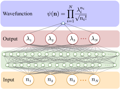
Figure 1: Visualization of the NCS approach. The input consists of Fock occupation numbers $n_{i}$ for each of bosonic modes $i=1,\ldots,N$, corresponding to discrete $k$ values $k_{i}$. The input is fed to a multilayer perceptron with arbitrary number and size of the hidden layers, see text for details. The number of neurons in the output layer is equal to the number of inputs ($k$-points). Each of the outputs $\lambda_{i}$, is transformed using the information from the input, $\lambda_{i}\rightarrow\lambda_{i}^{n_{i}}/\sqrt{n_{i}!}$. These numbers are multiplied to form the wavefunction $\psi$. All neurons in the hidden layers are densely connected to all neurons in the neighbouring layers; for clarity of the picture not all of them are visualized with grey lines.

II   Neural-network architecture.

We use a basis corresponding to bosonic occupations of the system with n denoting a single bosonic configuration of the whole system:

$$\ket{\textbf{n}}\equiv\ket{n_{1},n_{2},\ldots,n_{i},\ldots,n_{N}},$$ (1)

where $N$ is the number of discrete phonon modes considered. In an RBM architecture, $N$ is equal to the number of visible neurons. However, direct application of an RBM to non-additive systems is not efficient. This can easily been seen by writing the neural-network quantum state as $\ket{\psi(\mathbf{n})}=\psi(\hat{\mathbf{n}})\ket{\mathbf{n}}$; we have $[\psi(\hat{\mathbf{n}}),\hat{N}]=0$, $\hat{N}=\sum_{i}\hat{n}_{i}$ for a function $\psi(\mathbf{n})\sim\exp(E(\mathbf{\mathbf{n}}))$, $E$ being linear in $\mathbf{n}$. Hence, by construction an RBM operates in a sector of a given total number of particles.

To bypass this problem, we propose a neural network inspired from coherent states, which may be termed neural coherent states (NCS) and is illustrated in Fig. 1. Analogous to a standard coherent state, which for a given $n$ returns an output proportional to ${\lambda^{n}}/{\sqrt{{n}!}}$, with $\lambda$ being the parameter representing the coherent state, we construct a (mutilayer) feedforward neural network taking n as input. For each configuration, $N$ output numbers $\lambda_{i}$ are generated, which are subsequently transformed according to: $\lambda_{i}\rightarrow{{\lambda_{i}}^{n_{i}}}/{\sqrt{n_{i}!}}$. Then these numbers are multiplied to form the wavefunction. If the solution is exactly a coherent state $\lambda$ for each mode $i$, the network simply learns that $\lambda_{i}\equiv\lambda$ regardless of $n_{i}$. Correlated solutions are represented by perturbing the numbers $\lambda_{i}$, such that they depend on the input vector $\mathbf{n}$ in arbitrary way. This yields the variational Ansatz expressed as:

$$\innerproduct{\mathbf{n}}{\psi}=\psi(\mathbf{n})=\psi(n_{1},n_{2},\ldots,n_{N})=\prod\limits_{i=1}^{N}\frac{\lambda_{i}^{n_{i}}}{\sqrt{n_{i}!}},$$ (2)

where $\lambda_{i}$ is the output of a feedforward neural network (multilayer perceptron) with $M$ layers, i.e.:

$$\bm{\lambda}=\{\lambda_{1},\lambda_{2},\ldots,\lambda_{N}\}=h_{M}(h_{M-1}(\ldots h_{1}(\mathbf{n}))),$$ (3)

with each of the hidden layer transformations $h_{j}$ acting on output $\mathbf{h}_{j-1}$ of the previous layer:

$$h_{j}\left(\mathbf{h}_{j-1}\right)=\sigma\left(\mathbf{W}^{j-1}_{j}\mathbf{h}_{j-1}+\mathbf{b}_{j}\right)$$ (4)

where $\mathbf{W}^{j-1}_{j}$ and $\mathbf{b}_{j}$ are weights and bias of $j$-th layer, while $\sigma(x)$ is an activation function. This function, which introduces nonlinearity in the network, can be chosen from a wide range of classes, such as $\tanh$ (the choice made in this work), sigmoid or ReLU Nair and Hinton (2010).

With this Ansatz, we optimize the variational energy

$$\begin{split}E=&\frac{\bra{\psi}\hat{H}\ket{\psi}}{\innerproduct{\psi}{\psi}}=\frac{\sum\limits_{\mathbf{n},\mathbf{n}^{\prime}}\bra{\psi}\ket{\mathbf{n}}\matrixelement{\mathbf{n}}{\hat{H}}{\mathbf{n}^{\prime}}\bra{\mathbf{n}^{\prime}}\ket{\psi}}{\sum\limits_{\mathbf{n}}\bra{\psi}\ket{\mathbf{n}}\bra{\mathbf{n}}\ket{\psi}}=\\ =&\frac{\sum\limits_{\mathbf{n},\mathbf{n}^{\prime}}\psi^{*}(\mathbf{n}^{\prime})\hat{H}_{\mathbf{n^{\prime}n}}\psi(\mathbf{n})}{\sum\limits_{\mathbf{n}}|\psi(\mathbf{n})|^{2}}\end{split}$$ (5)

using Variational Monte Carlo, by sampling the probability distribution given by $\left|\psi(\mathbf{n})\right|^{2}$ .

III   Hamiltonian representation of impurity problems.

To test the efficiency of the NCS for non-additive systems, we focus on the Fröhlich Hamiltonian as given by:

$$\hat{H}=\frac{p^{2}}{2m}+\sum_{\mathbf{k}}\hbar\omega_{0}\hat{a}^{\dagger}_{\mathbf{k}}\hat{a}_{\mathbf{k}}+\sum_{\mathbf{k}}\left(V_{\mathbf{k}}\hat{a}_{\mathbf{k}}e^{-i\mathbf{k}\mathbf{r}}+V^{*}_{\mathbf{k}}\hat{a}_{\mathbf{k}}^{\dagger}e^{i\mathbf{k}\mathbf{r}}\right),$$ (6)

where $\mathbf{r}$ and $\mathbf{p}$ denote the position and momentum, respectively, of an impurity characterized by mass $m$. The three terms stand for impurity kinetic energy, bosonic bath energy and the impurity-bath interaction, respectively. The summation extends over all possible wavevectors $\mathbf{k}$.

Solution of this model is more convenient in the impurity frame, which is achieved by the Lee-Low-Pines transformation Lee et al. (1953). In the sector of zero total momentum, the Hamiltonian becomes:

$$\hat{H}=\frac{\left(-\sum\limits_{\mathbf{k}}\hbar\mathbf{k}\hat{a}^{\dagger}_{\mathbf{k}}\hat{a}_{\mathbf{k}}\right)^{2}}{2m}+\sum_{\mathbf{k}}\hbar\omega_{0}\hat{a}^{\dagger}_{\mathbf{k}}\hat{a}_{\mathbf{k}}+\sum_{\mathbf{k}}\left(V_{\mathbf{k}}\hat{a}_{\mathbf{k}}+V^{*}_{\mathbf{k}}\hat{a}_{\mathbf{k}}^{\dagger}\right).$$ (7)

The Lee-Low-Pines transformation removes the impurity degrees of freedom from the Hamiltonian. This maps the problem to a pure problem of interactions between the bosonic modes, at the price of introducing effective interactions between the phonon modes, described by the first term of the transformed Hamiltonian. The transformed impurity Hamiltonian problem is closer to the lattice boson problems such as the Bose-Hubbard problem, studied earlier with different NQS architectures Saito (2017); Saito and Kato (2017b). However, the problem mentioned earlier that the total number of bosons is not conserved, persists.

IV   Numerical results.

To make the Hamiltonian more convenient for numerical computation, we measure energy in units of $\hbar\omega_{0}$. Moreover, we discretize the $k$-grid to include $N$ points $k_{i}$ ranging from $-k_{0}$ to $k_{0}$ with step $\Delta k$. This finally puts the Hamiltonian into the following form in one dimension:

$$\hat{H}=\frac{\left(-\sum_{i}\hbar k_{i}\hat{a}_{k_{i}}^{\dagger}\hat{a}_{k_{i}}\right)^{2}}{2m}+\sum_{i}\hat{a}^{\dagger}_{k_{i}}\hat{a}_{k_{i}}+\sum_{i}\left(V_{k_{i}}\hat{a}_{k_{i}}+V^{*}_{k_{i}}\hat{a}_{k_{i}}^{\dagger}\right)$$ (8)

In the calculations we further restrict the maximum number of bosons at each mode at a value $n_{\text{max}}$, ranging between 3 and 8, depending on the parameter regime.

To benchmark our results, we compare them with two approaches – exact diagonalization, and the mean field approach Devreese (2016), where the ground state $\ket{\psi_{\textnormal{MF}}}$ is a direct product of coherent states, resulting in energy $E_{\textnormal{MF}}$:

$$\ket{\psi_{\textnormal{MF}}}=\bigotimes\limits_{i}\ket{-\frac{V_{k_{i}}}{1+\frac{\hbar^{2}k^{2}}{2m}}},E_{\text{MF}}=-\sum\limits_{k}\frac{|V_{k}|^{2}}{1+\frac{\hbar^{2}k^{2}}{2m}}.$$ (9)

By such choice of benchmarks, we are able to quantify the correlations expressed with our Ansatz.

As the first test, we take a small system with $N=2$ $k$-points $-k_{0}$ and $k_{0}$. We fix the impurity-bath potential at $V/(\hbar\omega_{0})=0.2$. Moreover, using convenient unit $m_{0}=\hbar k_{0}^{2}/(2\omega_{0})$ for the mass, such that $\hbar^{2}k_{0}^{2}/(2m_{0})=\hbar\omega_{0}$, we fix the inverse mass at $1/m=0.6\cdot(1/m_{0})$. We vary the number of nodes in the single hidden layer, thus changing the number of variational parameters and, consequently, the representative power of the network. For each number of nodes, we optimize the energy and compare the obtained energy with the ED and mean field energy mentioned above. The results are shown in Fig. 2.

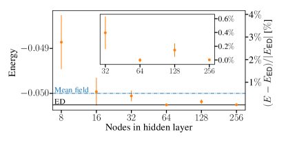
Figure 2: Representative power of the proposed approach. The optimized variational energy (orange dots, in units of $\hbar\omega_{0}$) is compared with exact diagonalization (ED), see right y-axis for percent scale relative to ED; and mean-field result for a system with 2 bosonic modes. The inset shows percent difference to ED for the four largest network sizes.

We observe that with the number of nodes high enough, the variational energy clearly goes below the mean-field one, proving the capability of our approach. For 64 and 256 nodes in the hidden layer, we have obtained an agreement with the ED result within the stochastic error of our variational approach.

To further evaluate the ability of NCS to express correlations between different bosonic modes, we study the performance of our approach with different impurity mass. Low mass is associated with high correlation level, while high mass brings the Hamiltonian closer to the infinite mass regime, where an analytic solution in the form of coherent state exists. We fix $V$ at $V/(\hbar\omega_{0})=0.2$. Then we optimize a network containing 1024 neurons in the hidden layer for different mass values and compare the result with the mean-field approach. The percentage deviation, $100\%\cdot(E-E_{\textnormal{ED}})/|E_{\textnormal{ED}}|$, for both the mean-field and NCS approach is shown in Fig. LABEL:fig:mass_V(a) as a function of the inverse mass.

Here, we observe very stable performance – the NCS is able to outperform mean-field approach across the range of (inverse) mass tested. Even at the intermediate regime, where mean-field solution lies $\approx 1.5\%$ above the ED, the NCS is able to accurately express the correlations and agree with ED within the stochastic error.

Next, we study the performance at different impurity-bath couplings $V$. We fix the inverse mass at $1/m=0.2\cdot(1/m_{0})$. Then we optimize the same network with 1024 neurons in the hidden layer for different values of $V$. The percentage deviation from ED, for both NCS and mean-field approach is shown in Fig. LABEL:fig:mass_V(b). Here we observe consistently good performance and clear advantage over mean-field across all values of impurity-bath coupling $V>0.1$. Data for $V<0.1$ is not shown, $E_{MF}-E_{ED}<10^{-5}$ and numerical errors in the gradients start to dominate the optimization, making it hard to reach more accurate results. We attribute this with a property of the NCS itself. For such small $V$, the system is very close to the vacuum state. When approaching the coherent state with $|\lambda|=\epsilon\ll 1$, leads to a dominance of states $\lambda_{i}=\epsilon$ for which $\epsilon^{0}=1$, independent on $\epsilon$. Importantly, our approach easily extends outside the weak-coupling regime, reaching equally accurate results for all $V$, even in the regime $V\sim 1$.

So far, all results are obtained for high maximum occupation numbers (up to $n_{\textnormal{max}}=8$) but only a small number of phonon modes. Next we gradually increase the number of $k$-points to benchmark the ability of the NCS approach to express the correlations between a larger number of bosonic modes, beyond a regime where ED is available. To this end we take $k$ being an equidistant grid between $-k_{0}$ and $k_{0}$ with a varying number of points. The constant impurity-bath interaction potential is $V_{k}\equiv 0.3$, which corresponds to contact interactions in real space, which is reasonable for one-dimensional systems. We fix the mass at $1/m=2\cdot(1/m_{0})$. Instead of the total energy, we are now interested in energy per number bosonic modes, to avoid a trivial scaling with the number of modes. In Fig. 4 we show the results of a benchmark against the mean-field approach and, where feasible, exact diagonalization.

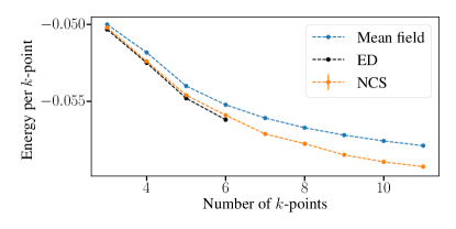
Figure 4: The energy divided by number of $k$-points calculated with the NCS approach as a function of the number of $k$-points on an equidistant grid between $k=-1$ and $k=1$. Error bars for NCS approach are smaller than point size. Dashed lines guide the eye.

We observe that the difference between the energy reached using our NCS state and the mean field solution increases with increasing the number of phonon modes, which is consistent with the fact that the amount of modes that are coupled to each other increases as well. Moreover, within the range where ED is feasible, we observe that the NCS results closely follow ED, while the mean-field energy is systematically higher. The number of network parameters in the single hidden layer network with 1024 hidden neurons used for training this system is much smaller ($\sim$2000 times smaller for 11 $k$-points) than the dimension of the Hilbert space, suggesting great potential to exploit this approach beyond the regime accessible with exact diagonalization.

V   Conclusions.

In summary, we introduced a new approach to solve non-additive systems with artificial neural networks. By benchmarking against exact diagonalization, we obtained accurate results for small systems and all parameter regimes studied. In particular, we were able to capture the challenging intermediate coupling regime at the same accuracy as weak-coupling results, illustrating that this method provides an unbiased approach to strong correlations in non-additive systems. Natural next steps include benchmarks against other methods for impurity systems and generalizations to other neural network architectures and more complex impurity models, such as the angulon quasiparticle Schmidt and Lemeshko (2015); Lemeshko (2017); Rzadkowski and Lemeshko (2018) which is the rotational counterpart of the polaron. The main complication is the non-commutative SO(3) algebra describing quantum rotations, which is inherently involved in the angulon problem. Some work in similar direction has already been done for spin models Vieijra et al. (2019), where irreducible representations of SU(2) were considered as inputs for the network. An appealing feature of variational neural network algorithms is their direct extension to unitary quantum dynamics of the system Carleo and Troyer (2017); Czischek et al. (2018); Fabiani and Mentink (2019); Schmitt and Heyl (2020); Hofmann et al. (2021). This requires generalizing the current approach to complex valued network parameters, yielding the possibility of extension of the presented work to the case of impurity dynamics, understanding of which is a subject of intensive ongoing research Ashida et al. (2018); Schiró (2010); Guo et al. (2020); Skou et al. (2021); Vasseur et al. (2013); Cherepanov et al. (2019).

We acknowledge fruitful discussions with Giacomo Bighin, Giammarco Fabiani, Areg Ghazaryan, Christoph Lampert, and Artem Volosniev at various stages of this work. W.R. is a recipient of a DOC Fellowship of the Austrian Academy of Sciences and has received funding from the EU Horizon 2020 programme under the Marie Skłodowska-Curie Grant Agreement No. 665385. M. L. acknowledges support by the European Research Council (ERC) Starting Grant No. 801770 (ANGULON). This work is part of the Shell-NWO/FOM-initiative “Computational sciences for energy research” of Shell and Chemical Sciences, Earth and Life Sciences, Physical Sciences, FOM and STW.

References

- Biamonte et al. (2017) J. Biamonte, P. Wittek, N. Pancotti, P. Rebentrost, N. Wiebe, and S. Lloyd, Nature 549, 195 (2017).
- Carleo et al. (2019) G. Carleo, I. Cirac, K. Cranmer, L. Daudet, M. Schuld, N. Tishby, L. Vogt-Maranto, and L. Zdeborová, Reviews of Modern Physics 91, 045002 (2019).
- Buffoni and Caruso (2021) L. Buffoni and F. Caruso, EPL (Europhysics Letters) 132, 60004 (2021).
- Carleo and Troyer (2017) G. Carleo and M. Troyer, Science 355, 602 (2017).
- Saito (2017) H. Saito, Journal of the Physical Society of Japan 86, 093001 (2017).
- Saito and Kato (2017a) H. Saito and M. Kato, Journal of the Physical Society of Japan 87, 014001 (2017a).
- Nomura et al. (2017) Y. Nomura, A. S. Darmawan, Y. Yamaji, and M. Imada, Phys. Rev. B 96, 205152 (2017), URL https://link.aps.org/doi/10.1103/PhysRevB.96.205152.
- Cai and Liu (2018) Z. Cai and J. Liu, Physical Review B 97, 035116 (2018).
- Choo et al. (2020) K. Choo, A. Mezzacapo, and G. Carleo, Nature communications 11, 1 (2020).
- Torlai and Melko (2018) G. Torlai and R. G. Melko, Phys. Rev. Lett. 120, 240503 (2018), URL https://link.aps.org/doi/10.1103/PhysRevLett.120.240503.
- Hartmann and Carleo (2019) M. J. Hartmann and G. Carleo, Phys. Rev. Lett. 122, 250502 (2019), URL https://link.aps.org/doi/10.1103/PhysRevLett.122.250502.
- Yoshioka and Hamazaki (2019) N. Yoshioka and R. Hamazaki, Phys. Rev. B 99, 214306 (2019), URL https://link.aps.org/doi/10.1103/PhysRevB.99.214306.
- Vicentini et al. (2019) F. Vicentini, A. Biella, N. Regnault, and C. Ciuti, Phys. Rev. Lett. 122, 250503 (2019), URL https://link.aps.org/doi/10.1103/PhysRevLett.122.250503.
- Irikura and Saito (2020) N. Irikura and H. Saito, Phys. Rev. Research 2, 013284 (2020), URL https://link.aps.org/doi/10.1103/PhysRevResearch.2.013284.
- Holstein (1959) T. Holstein, Annals of physics 8, 325 (1959).
- Fröhlich (1954) H. Fröhlich, Advances in Physics 3, 325 (1954).
- Su et al. (1979) W. Su, J. Schrieffer, and A. J. Heeger, Physical review letters 42, 1698 (1979).
- Su et al. (1980) W.-P. Su, J. Schrieffer, and A. Heeger, Physical Review B 22, 2099 (1980).
- Hepp and Lieb (1973) K. Hepp and E. H. Lieb, Annals of Physics 76, 360 (1973), ISSN 0003-4916, URL https://www.sciencedirect.com/science/article/pii/0003491673900390.
- Dicke (1954) R. H. Dicke, Phys. Rev. 93, 99 (1954), URL https://link.aps.org/doi/10.1103/PhysRev.93.99.
- Anderson (1961) P. W. Anderson, Phys. Rev. 124, 41 (1961), URL https://link.aps.org/doi/10.1103/PhysRev.124.41.
- Melko et al. (2019) R. G. Melko, G. Carleo, J. Carrasquilla, and J. I. Cirac, Nature Physics 15, 887 (2019).
- Deng et al. (2017) D.-L. Deng, X. Li, and S. Das Sarma, Phys. Rev. X 7, 021021 (2017), URL https://link.aps.org/doi/10.1103/PhysRevX.7.021021.
- Ohgoe and Imada (2014) T. Ohgoe and M. Imada, Physical Review B 89, 195139 (2014).
- Karakuzu et al. (2017) S. Karakuzu, L. F. Tocchio, S. Sorella, and F. Becca, Phys. Rev. B 96, 205145 (2017), URL https://link.aps.org/doi/10.1103/PhysRevB.96.205145.
- Ferrari et al. (2020) F. Ferrari, R. Valentí, and F. Becca, Phys. Rev. B 102, 125149 (2020), URL https://link.aps.org/doi/10.1103/PhysRevB.102.125149.
- Vargas-Hernández et al. (2018) R. A. Vargas-Hernández, J. Sous, M. Berciu, and R. V. Krems, Phys. Rev. Lett. 121, 255702 (2018), URL https://link.aps.org/doi/10.1103/PhysRevLett.121.255702.
- Arsenault et al. (2014) L.-F. m. c. Arsenault, A. Lopez-Bezanilla, O. A. von Lilienfeld, and A. J. Millis, Phys. Rev. B 90, 155136 (2014), URL https://link.aps.org/doi/10.1103/PhysRevB.90.155136.
- Rigo and Mitchell (2020) J. B. Rigo and A. K. Mitchell, Phys. Rev. B 101, 241105 (2020), URL https://link.aps.org/doi/10.1103/PhysRevB.101.241105.
- Glauber (1963) R. J. Glauber, Phys. Rev. 131, 2766 (1963), URL https://link.aps.org/doi/10.1103/PhysRev.131.2766.
- Nair and Hinton (2010) V. Nair and G. E. Hinton, in Icml (2010).
- Lee et al. (1953) T. Lee, F. Low, and D. Pines, Physical Review 90, 297 (1953).
- Saito and Kato (2017b) H. Saito and M. Kato, Journal of the Physical Society of Japan 87, 014001 (2017b).
- Devreese (2016) J. Devreese, arXiv preprint arXiv:1611.06122 (2016).
- Schmidt and Lemeshko (2015) R. Schmidt and M. Lemeshko, Physical review letters 114, 203001 (2015).
- Lemeshko (2017) M. Lemeshko, Physical review letters 118, 095301 (2017).
- Rzadkowski and Lemeshko (2018) W. Rzadkowski and M. Lemeshko, The Journal of chemical physics 148, 104307 (2018).
- Vieijra et al. (2019) T. Vieijra, C. Casert, J. Nys, W. De Neve, J. Haegeman, J. Ryckebusch, and F. Verstraete, arXiv preprint arXiv:1905.06034 (2019).
- Czischek et al. (2018) S. Czischek, M. Gärttner, and T. Gasenzer, Phys. Rev. B 98, 024311 (2018), URL https://link.aps.org/doi/10.1103/PhysRevB.98.024311.
- Fabiani and Mentink (2019) G. Fabiani and J. H. Mentink, SciPost Phys. 7, 4 (2019), URL https://scipost.org/10.21468/SciPostPhys.7.1.004.
- Schmitt and Heyl (2020) M. Schmitt and M. Heyl, Phys. Rev. Lett. 125, 100503 (2020), URL https://link.aps.org/doi/10.1103/PhysRevLett.125.100503.
- Hofmann et al. (2021) D. Hofmann, G. Fabiani, J. H. Mentink, G. Carleo, and M. A. Sentef, arXiv preprint arXiv:2105.01054 (2021).
- Ashida et al. (2018) Y. Ashida, T. Shi, M. C. Bañuls, J. I. Cirac, and E. Demler, Phys. Rev. Lett. 121, 026805 (2018), URL https://link.aps.org/doi/10.1103/PhysRevLett.121.026805.
- Schiró (2010) M. Schiró, Phys. Rev. B 81, 085126 (2010), URL https://link.aps.org/doi/10.1103/PhysRevB.81.085126.
- Guo et al. (2020) C. Guo, X. Meng, H. Fu, Q. Wang, H. Wang, Y. Tian, J. Peng, R. Ma, Y. Weng, S. Meng, et al., Phys. Rev. Lett. 124, 206801 (2020), URL https://link.aps.org/doi/10.1103/PhysRevLett.124.206801.
- Skou et al. (2021) M. G. Skou, T. G. Skov, N. B. Jørgensen, K. K. Nielsen, A. Camacho-Guardian, T. Pohl, G. M. Bruun, and J. J. Arlt, Nature Physics pp. 1–5 (2021).
- Vasseur et al. (2013) R. Vasseur, K. Trinh, S. Haas, and H. Saleur, Phys. Rev. Lett. 110, 240601 (2013), URL https://link.aps.org/doi/10.1103/PhysRevLett.110.240601.
- Cherepanov et al. (2019) I. N. Cherepanov, G. Bighin, L. Christiansen, A. V. Jørgensen, R. Schmidt, H. Stapelfeldt, and M. Lemeshko, arXiv preprint arXiv:1906.12238 (2019).