Calculation of Berry curvature using nonorthogonal atomic orbitals
Abstract
We present a derivation of the full formula to calculate the Berry curvature on non-orthogonal numerical atomic orbital (NAO) bases. Because usually, the number of NAOs is larger than that of the Wannier bases, we use a orbital contraction method to reduce the basis sizes, which can greatly improve the calculation efficiency without significantly reducing the calculation accuracy. We benchmark the formula by calculating the Berry curvature of ferroelectric BaTiO3 and bcc Fe, as well as the anomalous Hall conductivity (AHC) for Fe. The results are in excellent agreement with the finite difference and previous results in the literature. We find that there are corrections terms to the Kubo formula of the Berry curvature. For the full NAO base, the differences between the two methods are negligibly small, but for the reduced bases sets, the correction terms become larger, which may not be neglected in some cases. The formula developed in this work can readily be applied to the non-orthogonal generalized Wannier functions.
1 Introduction
Berry curvature is of fundamental importance for understanding some basic properties of solid materials and is essential for the description of the dynamics of Bloch electrons [1, 2]. It acts as a magnetic field in momentum space, which leads to some anomalous transport effects, including the first order[3, 4, 5, 6, 7, 1, 8], and second order[9, 10, 11, 12, 13] anomalous Hall effects (AHE). It may introduce shift current in polar materials [14, 15, 16, 17]. Berry curvature also plays a crucial role in the classification of topological materials [18, 19, 20].
The first-principles calculations of the Berry curvature and the anomalous Hall conductivity (AHC) have been reviewed in Ref. [21]. Especially, the Berry curvature and AHC have been calculated via the Kubo formula [5, 6]. However, this method requires to calculate band structures at very dense points, and sum over a large number of unoccupied states to converge the results. Therefore the computational cost is very high, even for simple materials. Vanderbilt and co-works developed a very efficient interpolation scheme [22] to calculate Berry curvature and AHC [23, 24] based on maximally localized Wannier functions (MLWFs)[25, 26], which has been demonstrated to calculate the AHC to very high accuracy with only a tiny fraction of time of the original Kubo formula. However, it is not always easy to construct high-quality MLWFs, for complex systems. More seriously, in some cases, the MLWFs may not respect the point group symmetries of the crystal. Breaking of the symmetry may lead to qualitatively incorrect results. Special attention has to be paid to construct the symmetry adapted MLWFs [26, 27, 28].
Recently, Lee at. el. derived the Kubo formula of optical matrices as well as Berry curvature using nonorthogonal numerical atomic orbitals (NAOs) [29]. Wang et. al. also derived the formula of Berry connection and its higher order derivatives based on NAOs [17]. The NAOs are strictly localized and more importantly, have spherical symmetries, and therefore, no extra effort is needed to construct the symmetry-adapted MLWFs. This is of great advantage for the applications in complex systems. In this work, we derive the full formula to calculate the Berry curvature bases on NAOs [30]. We show that in the full derivation of Berry curvature, there are correction terms to the Kubo formula[29] on the NAO bases. Since the number of NAOs is usually larger than that of the MLWFs, we use a orbital contraction technique to reduce the number of NAOs, which can greatly improve the calculation efficiency without significantly reducing the calculation accuracy. These correction terms are small if a large NAO base is used, however, for the reduced NAO bases, the corrections are not negligible in some cases. The formula developed in this work can be directly applied to the non-orthogonal generalized Wannier functions, which, if constructed properly, are typically more localized than the orthogonal Wannier functions [31].
The rest of the paper is organized as follows. In Sec. 2, we present the derivation of Berry curvature for non-orthogonal NAOs, followed by detailed benchmark calculations of Berry curvature for BaTiO3 and AHC for Fe in Sec. 3. In Sec. 4, we introduce a technique to reduce the number of NAOs to accelerate Berry curvature calculations. We summarize in Sec. 5.
2 Berry curvature in non-orthogonal atomic bases
2.1 Derivation of Berry curvature formula
The derivation of Berry curvature formula expressed in a non-orthogonal NAO basis is similar to that of the orthogonal Wannier bases, but there are also some considerable differences. The derivation is transparent for people who are not familiar with the Wannier functions.
We start from the definition of the Berry curvature [2],
| (1) |
where,
| (2) |
is the Berry connection, and are the cell-periodic Bloch functions, whose expression on a NAO basis is given by Eq. (33) in the Appendix.
More generally, one may generalize the above definition of Berry connection and Berry curvature to a multi-bands case,
| (3) |
and
| (4) | |||||
where .
To simplify the above equation, we introduce a dipole matrix , as follows,
| (6) |
where the superscript “” in refers to that the dipole matrix is summed over the lattice . This quantity is similar to the in Ref. [22]. While it is somehow cumbersome to calculate the dipole matrix in the Wannier bases, can be easily calculated by two-center integrals on the NAO bases by taking the advantages of the spherical symmetry of the NAOs[32, 33].
One part of the contribution to the Berry curvature is from the dipole matrix,
| (7) |
which is due to the lack of inversion symmetry of the crystal.
The other contribution to the Berry curvature comes from the change of the Bloch wave function coefficient with . Following Ref. [22], we may also introduce a matrix in the non-orthogonal NAO bases, as follows,
| (8) |
There are useful relations between and , and , and the proof is given in the Appendix.
| (9) | |||||
| (10) |
where
| (11) |
For the orthogonal Wannier bases, where =0, we have , and , i.e, is Hermitian, and is anti-Hermitian in the orthogonal Wannier bases. It is easy to show that Berry connection .
We can simplify Eq. (5) by inserting the identity matrix,
| (12) |
For example, for the second term on the right side of Eq. (5), we have,
| (13) |
After some derivation, we obtain the formula of the Berry curvature in the non-orthogonal NAO bases,
| (14) | |||||
where
| (15) |
We note that Eq. (14) is very similar to Eq. (27) in Ref. [22], but also with notable differences. Because is not Hermitian, and is not anti-Hermitian for the non-orthogonal NAO bases, we cannot write the equation in the form of commutators as Eq. (27) in Ref. [22].
2.2 Calculation of matrix
From the linear response theory given in Appendix A, one obtains[17] (for ),
| (16) |
where
| (17) |
There is some freedom to choose . However, since , it must satisfy the following constrain,
| (18) |
For the orthogonal bases, one can just take [22]. However, this choice is generally not feasible for the nonorthogonal base. Instead, we can use the parallel transport gauge, , i.e., . Using the relation, , and the relations in Eq. (9) and Eq. (10) for =, we can easily prove that the parallel transport gauge, automatically satisfies the constrain of Eq. (18). Note that the parallel transport gauge defined here for the cell-periodic functions is different from the “parallel transport gauge” in Ref.[22] for the state vectors in the “tight-binding space” of the MLWFs. As shown in the next section, would not appear in the Berry curvature calculations, and therefore the choice of particular gauge would not change the Berry curvature, but it may affect the Berry connection.
2.3 Total Berry curvature
The total Berry curvature is calculated as follows,
| (19) |
where, is the Fermi occupation function. To avoid the numerical instability caused by the canceling contributions of large values of [see Eq. (16)], originated from the small energy splitting between a pair of occupied bands and , we would like to sperate the summation between the occupied and unoccupied states, similar to the MLWF interpolation method[22]. However, this is a little bit more tricky for the non-orthogonal bases.
We first rewrite Eq. (14) by replacing and with and using Eq. (10),
| (20) | |||||
where the first four terms closely resemble those of Eq. (27) in Ref.[22]. One can proof the Berry curvature defined above is gauge invariant (see Appendix A3). In this form, the contribution from matrices are exactly canceled for a pair of occupied states , . The last term is due to the non-orthogonality of the NAO bases. We can therefore calculate the total Berry curvature as [22],
| (21) | |||||
We immediately see that for the orthogonal bases, the last line in the above equation vanishes, and the total Berry curvature reduces to Eq. (32) in Ref.[22].
2.4 Comparison with the naive Kubo formula
The Berry curvatures are often calculated via the naive Kubo formula [21, 29],
| (22) |
where is the velocity matrix. According to Ref. [34, 35], we have
| (23) |
where the Berry connection . One easily obtain the velocity operator matrix for ,
| (24) |
which is identical to that derived in Ref. [29] via a different approach.
By comparing Eq. (21) and Eq. (22), one finds that the full Berry curvature actually includes some correction terms to the naive Kubo formula, i.e., , and,
| (25) | |||||
where is defined in Eq. (15). These additional terms are also presented in the MLWF bases [22]. These correction terms come from the incompleteness of the tight-binding bases to the original Hilbert space [36, 37]. Even though the contributions of are often very small, and sometimes negligible, it is still useful to have a strict formula to compare with. This will be further addressed in the following sections.
3 Results and discussion
We take BaTiO3 and ferromagnetic Fe as examples to benchmark the calculation of the Berry curvature using NAOs. These choices represent two typical systems where Berry curvature is nonzero that either break the inversion symmetry (BaTiO3) or time-reversal symmetry (Fe). While the SOC is not needed for BaTiO3 to get nonzero Berry curvature, it is essential for Fe to have nonzero Berry curvature, which is well explained in Ref.[2]
3.1 Computational details
We first perform self-consistent density functional theory calculation implemented in the Atomic-orbtial Based Ab-initio Computation at UStc (ABACUS) code [30, 32]. The generalized gradient approximation in the Perdew-Burke-Ernzerhof (PBE) [38] form is adopted. We adopt optimized norm-conserving Vanderbilt [39] multi-projector, SG15 pseudopotentials [40, 41].
For the BaTiO3, the 5s25p65d16s1 electrons for Ba, the 2s23p64s23d2 electrons for Ti, and the 2s22p4 electrons for O are treated as valence electrons. The cutoff energy for the wave function is set to 60 Ry. A -mesh is used in the self-consistent calculations. The NAO bases for Ba, Ti, O are 4s2p2d, 4s2p2d1f, 2s2p1d, respectively.
For bcc Fe, the 3s23p64s23d6 electrons are included self-consistently. Spin-orbit interactions are tuned on. The cutoff energy for the wave function is set to 120 Ry. A 161616 -mesh is used in the self-consistent calculations. The NAOs of Fe is 4s2p2d1f.
After the self-consistent calculations, the tight-binding Hamiltonian and overlap matrices in the NAO bases, which are generated during the self-consistent calculations, are readily outputted and are used for the Berry curvature calculations.
3.2 Berry curvature of BaTiO3
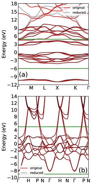
As the first example, we calculate the Berry curvature of rhombohedral BaTiO3 with space group (No. 160, Rhombohedral axes). The lattice constant = 4.081 Å, and = 89.66∘ are used. The Wyckoff positions are given in Table 1. BTO is a ferroelectric insulator without inversion symmetry. The band structures of BaTiO3 near the Fermi level =0 are shown in red solid lines in Fig. 1(a).
| Wyckoff position | ||||
|---|---|---|---|---|
| Ba | 0.002 | 0.002 | 0.002 | 1a |
| Ti | 0.516 | 0.516 | 0.516 | 1a |
| O | 0.974 | 0.485 | 0.485 | 3b |
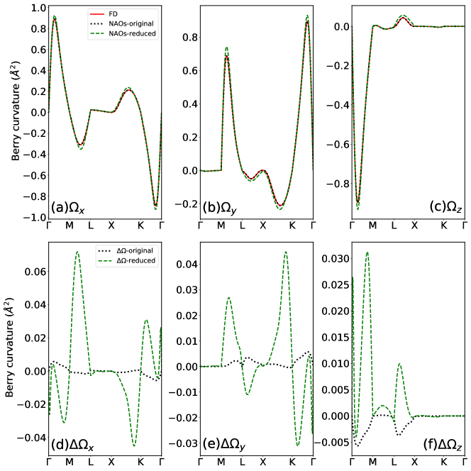
Figure 2(a)-(c) depict the Berry curvatures of BaTiO3 along the , and -axes respectively, where
| (26) |
The Berry curvatures calculated by Eq. (21) are shown in the black dashed lines. We compared the results to those calculated by the finite-difference (FD) method via Eq. (46), which are shown in the solid red lines. As we see, the Berry curvatures calculated by the Eq. (21) are in excellent agreement with the FD method.
Figure 2(d)-(f) show the differences between this work and Kubo formula of BaTiO3 along the , and -axes respectively, in black solid lines. As seen from the figure, is extremely small, which are less than 1% of the total Berry curvature. These results suggest that the NAO bases used in the calculations are rather complete for this problem.
3.3 AHC of Fe
In this section, we calculate the Berry curvature and the AHC for bcc Fe. The lattice constant of bcc Fe is taken as = 2.870 Å. The band structure of Fe is shown in Fig. 1(b) in red solid lines around Fermi level =0.
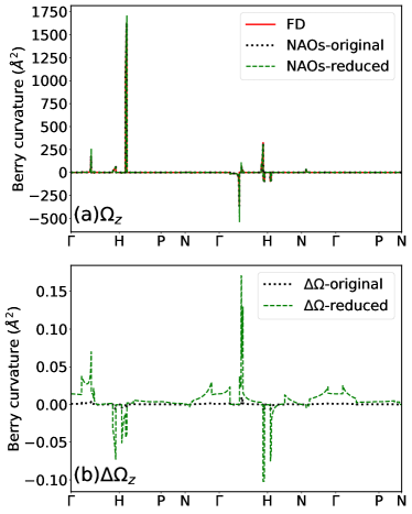
The Berry curvature of bcc Fe along the -axis is given in Fig. 3(a). The black dotted line is the Berry curvature calculated via Eq. (21), which is in excellent agreement with the Berry curvature calculated via FD method, shown in the red solid line. For most points, the Berry curvature is very small except at a few points, which have huge Berry curvature, due to the spin-orbit-split avoided crossings near the Fermi level [6, 22].
We then calculate the dc anomalous Hall conductivity (AHC) [23, 24],
| (27) |
To calculate the AHC of bcc Fe, a 300300300 -mesh is used and if the Berry curvature of a certain point is greater than 100 Å2, the Berry curvature is recalculated at a refined 777 submesh around the point, following the scheme of Ref. [6, 22]. The calculated AHC for Fe is 738 ( cm)-1. This result is in good agreement with 751 (cm)-1, obtained from full-potential all-electron calculations by Yao et. al. [6], which is also close to 756 ( cm)-1 obtained from normal conserving pseudopotential calculations via Wannier interpolation techniques [22]. The Fe pseudopotential in Ref. [22] is specially optimized to reproduce the all-electron result of AHC, and the difference between this work and Ref. [22] might come from the different pseudopotentials used in the calculations.
4 Berry curvatures calculated with reduced basis sets
In the previous section, we showed that the Berry curvatures calculated by Eq. (21) are in excellent agreement with FD results. However, the NAO basis sets have too many orbitals compared to the Wannier bases, and therefore computationally more expensive. We would like to reduce the basis size to accelerate the calculations, but maintain the accuracy. The idea is to use reduced basis sets, to reproduce the band structures in a smaller energy window. This is done via a revised band interpolation technique [42] via NAOs.
To reduce the number of NAOs, we reconstruct a new set of NAOs as the linear combination of original on-site orbitals, i.e,
| (28) |
where is the -th orbit of the -th atom. One of the problems of the maximally localized Wannier functions is that their centers are not necessarily on atom positions or other high-symmetry points[27]. In contrast, the reduced NAOs are linear combinations of on-site NAOs, so they are still atom centered and strictly localized. The number of the reduced NAO bases , is less than the number of . is a real orthogonal matrix to keep the reduced NAOs real.
We obtained the reduced NAOs by minimizing the spillage between the wave functions calculated by original NAOs and the reduced basis set at a coarse -mesh in a chosen energy window. Details of this process are given in B.
4.0.1 BaTiO3
Figure 1(a) compares the band structure of BaTiO3 calculated by the original bases (solid red lines) and the reduced bases (black dashed lines). The reduced bases set is optimized by fitting the wave functions in the energy window of -6 to 4.8 eV (The energy window is represented by a solid green line) which covers the lowest three bands above the Fermi level. A uniform grid of 888 -mesh is used to generate the reduced basis set. The reduced base has 38 orbitals compared to the 86 orbitals in the original bases. As we see from Fig. 1(a), the band structures calculated by the reduced bases are in excellent agreement with the original band structures within the energy window. The lower energy bands above the energy window also agree very well. For the bands far above the energy window, the agreement becomes worse as expected.
The Berry curvatures of BaTiO3 calculated by the reduced bases are shown in green dashed lines in Fig. 2(a)-(c), compared to those calculated by the original bases. The overall agreement is rather good, with only small differences at some -point.
We now check the for the reduced bases, depicted in Fig. 2(d)-(e), which are shown in green dashed lines. We see that for the reduced basis, is significantly larger than that of the full basis calculations, which suggests that if a reduced basis is used, the corrections to the Kubo formula may not be ignored in some cases. One may expect that if an even smaller non-orthogonal Wannier bases are used, the correction may have an even larger contribution, which cannot be ignored.
4.0.2 bcc Fe
The reduced basis set of the Fig. 1(b) is optimized in the energy window of -9 5 eV, on a uniform grid of 888 -points. We obtain 28 orbitals (include spin) from the original 54 orbitals. The energy bands obtained by the reduced basis set are almost identical to the original bands. In fact, the agreement is still very well even outside the energy window, below 14 eV.
The Berry curvature calculated by the reduced bases are also shown in Fig. 3(a) in the green dashed line compared to the original result. There are only very small differences between the results obtained by the original and reduced bases. The correction to the naive Kubo formula for the reduced bases are shown in the green dashed line in Fig. 3(b). The correction is much larger than that for the original bases, shown in the black dotted line. However, the correction is still negligibly small compared to the total Berry curvature, because the dominant contribution to the contribution comes from the - terms [22].
The AHC of bcc Fe calculated by the reduced basis set is 734 ( cm)-1, which is in good agreement with that calculated by the full basis set 738 ( cm)-1.
5 Summary
We derive the formula to calculate the Berry curvature using non-orthogonal NAOs. We find that there are some additional correction terms besides the usual Kubo formula. We calculate the Berry curvature of Rhombohedral BaTiO3 and bcc Fe, as well as the AHC for Fe. The results are in excellent agreement with the finite difference method. We develop a method that can significantly reduce the number of orbitals in the NAO bases but can still maintain the accuracy of the calculations. We also compare the Berry curvature and AHC calculated via our formula and the Kubo formula. We find for the original basis, the differences between the two methods are negligibly small, but for the reduced bases sets, the correction terms become larger. The methods developed in this work can be applied to non-orthogonal generalized Wannier functions.
Appendix A Electronic structure by LCAO
In the NAO basis, the Hamiltonian matrix is calculated as,
| (29) |
where is a short notation of the -th NAO in the -th unit cell, i.e., , and is the center of the orbital. The Hamiltonian is self-consistently determined by the Kohn-Sham equations. In general, the NAOs are not orthogonal to each other, and their overlap matrix is
| (30) |
Therefore, in the NAO bases, the corresponding Kohn-Sham equation (under the converged charge density) is
| (31) |
The Bloch wave function is,
| (32) |
and the corresponding cell-periodic part is
| (33) |
A.1 Linear response theory in non-orthogonal NAO bases
According to the perturbation theory, we derive the first-order term of Eq. (31) with respect to the parameter in the non-degenerate case,
| (34) |
We use set to expand , i.e.,
| (35) |
Multiply to the left of Eq. (34), we have
| (36) |
We obtain for ,
| (37) |
Generally, for the non-orthogonal bases,
| (38) |
and can be determined by choice of a particular gauge as discussed in Sec. 2.2.
A.2 Relations between and , and
A.3 Proof of gauge invariance of Berry curvature
We prove the Berry curvature defined in Eq. (20) is gauge invariant. When is changed to , the corresponding , , matrix will change to,
| (44) |
The fourth term in Eq. (20) becomes
| (45) | |||||
i.e., it is invariant under the gauge change. Similarly, we can prove that all other terms of Eq. (20) are also gauge invariant, and therefore the Berry curvature is gauge invariant.
A.4 Calculating the Berry curvature by finite difference
The Berry curvature can be calculated via the finite difference method, using the relationship between Berry phase and Berry curvature [2],
| (46) |
We choose a small square loop around a point in the Brillouin Zone and calculate the discretized Berry phase [43] of the loop. The Berry curvature at the given point can be obtained as =, where is the normal direction of the square loop and is its area. In principles the Berry phase is correct only modulo 2. [2] But here, we have no ambiguity of chosen the correct branches, as is significantly smaller than the quanta when is very small.
Appendix B Optimize the reduced bases
The reduced bases orbitals are obtained by minimizing the spillage between the reduced bases and the Bloch wave functions in the selected energy window and points. The spillage [42] is defined as,
| (47) |
where is the energy bands within the energy window. is a projector spanned by the reduced NAOs,
| (48) |
where, is the overlap matrix of the reduced NAOs. The reduced NAOs are the linear combination of the on-site original NAOs. Using Eq. (28), we have,
| (49) |
where is the overlap matrix of the original NAOs. The spillage can be written as,
| (50) |
Using the rule,
| (51) |
where is an invertible matrix, we get the derivative of to the matrix,
| (52) |
Once we have the gradients, we optimize the spillage via the Broyden–Fletcher–Goldfarb–Shanno (BFGS) method implemented in the numpy [44] and scipy package.[45] To determine the initial reduced NAOs, we evaluate the coefficients of each orbital in the full bases of the wave functions in the selected energy window and -mesh. We keep the NAOs, whose coefficients are larger than some threshold as the initial reduced NAOs, which give the corresponding initial matrices. We then minimize the spillage to obtain the optimized NAOs. When optimize the matrix using Eq. (52), the wave functions , overlap matrix , and initial matrix all have the point group symmetry, and therefore in principle, the reduced NAOs should still preserve the symmetry. However, there might be small symmetry breaking, due to numerical noise. The reduced NAOs can be symmetrized using the algorithms of Ref. [27] if necessary.
References
References
- [1] Di Xiao, Ming-Che Chang, and Qian Niu. Berry phase effects on electronic properties. Rev. Mod. Phys., 82:1959–2007, Jul 2010.
- [2] David Vanderbilt. Berry Phases in Electronic Structure Theory: Electric Polarization, Orbital Magnetization and Topological Insulators. Cambridge University Press, 2018.
- [3] T. Jungwirth, Qian Niu, and A. H. MacDonald. Anomalous hall effect in ferromagnetic semiconductors. Phys. Rev. Lett., 88:207208, May 2002.
- [4] Masaru Onoda and Naoto Nagaosa. Topological nature of anomalous hall effect in ferromagnets. Journal of the Physical Society of Japan, 71(1):19–22, 2002.
- [5] Zhong Fang, Naoto Nagaosa, Kei S. Takahashi, Atsushi Asamitsu, Roland Mathieu, Takeshi Ogasawara, Hiroyuki Yamada, Masashi Kawasaki, Yoshinori Tokura, and Kiyoyuki Terakura. The anomalous hall effect and magnetic monopoles in momentum space. Science, 302(5642):92–95, 2003.
- [6] Yugui Yao, Leonard Kleinman, A. H. MacDonald, Jairo Sinova, T. Jungwirth, Ding-sheng Wang, Enge Wang, and Qian Niu. First principles calculation of anomalous hall conductivity in ferromagnetic bcc fe. Phys. Rev. Lett., 92:037204, Jan 2004.
- [7] Naoto Nagaosa, Jairo Sinova, Shigeki Onoda, A. H. MacDonald, and N. P. Ong. Anomalous hall effect. Rev. Mod. Phys., 82:1539–1592, May 2010.
- [8] Hongming Weng, Rui Yu, Xiao Hu, Xi Dai, and Zhong Fang. Quantum anomalous hall effect and related topological electronic states. Advances in Physics, 64(3):227–282, 2015.
- [9] Inti Sodemann and Liang Fu. Quantum nonlinear hall effect induced by berry curvature dipole in time-reversal invariant materials. Phys. Rev. Lett., 115:216806, Nov 2015.
- [10] Yang Zhang, Yan Sun, and Binghai Yan. Berry curvature dipole in weyl semimetal materials: An ab initio study. Phys. Rev. B, 97:041101, Jan 2018.
- [11] Yang Zhang, Jeroen van den Brink, Claudia Felser, and Binghai Yan. Electrically tuneable nonlinear anomalous hall effect in two-dimensional transition-metal dichalcogenides WTe 2 and MoTe 2. 2D Materials, 5(4):044001, jul 2018.
- [12] Jhih-Shih You, Shiang Fang, Su-Yang Xu, Efthimios Kaxiras, and Tony Low. Berry curvature dipole current in the transition metal dichalcogenides family. Phys. Rev. B, 98:121109, Sep 2018.
- [13] Qiong Ma, Su-Yang Xu, Huitao Shen, David Macneill, Valla Fatemi, Tay-Rong Chang, Andrés M. Mier Valdivia, Sanfeng Wu, Zongzheng Du, Chuang-Han Hsu, and et al. Observation of the nonlinear hall effect under time-reversal-symmetric conditions. Nature, 565(7739):337–342, 2019.
- [14] J. E. Sipe and A. I. Shkrebtii. Second-order optical response in semiconductors. Phys. Rev. B, 61:5337–5352, Feb 2000.
- [15] Steve M. Young and Andrew M. Rappe. First principles calculation of the shift current photovoltaic effect in ferroelectrics. Phys. Rev. Lett., 109:116601, Sep 2012.
- [16] Liang Z Tan, Fan Zheng, Steve M Young, Fenggong Wang, Shi Liu, and Andrew M Rappe. Shift current bulk photovoltaic effect in polar materials—hybrid and oxide perovskites and beyond. npj Computational Materials, 2(1):16026, 2016.
- [17] Chong Wang, Sibo Zhao, Xiaomi Guo, Xinguo Ren, Bing-Lin Gu, Yong Xu, and Wenhui Duan. First-principles calculation of optical responses based on nonorthogonal localized orbitals. New Journal of Physics, 21(9):093001, sep 2019.
- [18] M. Z. Hasan and C. L. Kane. Colloquium: Topological insulators. Rev. Mod. Phys., 82:3045–3067, Nov 2010.
- [19] Xiao-Liang Qi and Shou-Cheng Zhang. Topological insulators and superconductors. Rev. Mod. Phys., 83:1057–1110, Oct 2011.
- [20] C. L. Kane and E. J. Mele. topological order and the quantum spin hall effect. Phys. Rev. Lett., 95:146802, Sep 2005.
- [21] M Gradhand, D V Fedorov, F Pientka, P Zahn, I Mertig, and B L Györffy. First-principle calculations of the berry curvature of bloch states for charge and spin transport of electrons. Journal of Physics: Condensed Matter, 24(21):213202, may 2012.
- [22] Xinjie Wang, Jonathan R. Yates, Ivo Souza, and David Vanderbilt. Ab initio calculation of the anomalous hall conductivity by wannier interpolation. Phys. Rev. B, 74:195118, Nov 2006.
- [23] Ganesh Sundaram and Qian Niu. Wave-packet dynamics in slowly perturbed crystals: Gradient corrections and berry-phase effects. Phys. Rev. B, 59:14915–14925, Jun 1999.
- [24] E.N. Adams and E.I. Blount. Energy bands in the presence of an external force field—ii: Anomalous velocities. Journal of Physics and Chemistry of Solids, 10(4):286 – 303, 1959.
- [25] Nicola Marzari and David Vanderbilt. Maximally localized generalized wannier functions for composite energy bands. Phys. Rev. B, 56:12847–12865, Nov 1997.
- [26] Ivo Souza, Nicola Marzari, and David Vanderbilt. Maximally localized wannier functions for entangled energy bands. Phys. Rev. B, 65:035109, Dec 2001.
- [27] R. Sakuma. Symmetry-adapted wannier functions in the maximal localization procedure. Phys. Rev. B, 87:235109, Jun 2013.
- [28] K. S. Thygesen, L. B. Hansen, and K. W. Jacobsen. Partly occupied wannier functions: Construction and applications. Phys. Rev. B, 72:125119, Sep 2005.
- [29] Chi-Cheng Lee, Yung-Ting Lee, Masahiro Fukuda, and Taisuke Ozaki. Tight-binding calculations of optical matrix elements for conductivity using nonorthogonal atomic orbitals: Anomalous hall conductivity in bcc fe. Phys. Rev. B, 98:115115, Sep 2018.
- [30] Mohan Chen, G-C Guo, and Lixin He. Systematically improvable optimized atomic basis sets forab initiocalculations. Journal of Physics: Condensed Matter, 22(44):445501, oct 2010.
- [31] Lixin He and David Vanderbilt. Exponential decay properties of wannier functions and related quantities. Phys. Rev. Lett., 86:5341–5344, 2001.
- [32] Pengfei Li, Xiaohui Liu, Mohan Chen, Peize Lin, Xinguo Ren, Lin Lin, Chao Yang, and Lixin He. Large-scale ab initio simulations based on systematically improvable atomic basis. Computational Materials Science, 112:503 – 517, 2016.
- [33] José M Soler, Emilio Artacho, Julian D Gale, Alberto García, Javier Junquera, Pablo Ordejón, and Daniel Sánchez-Portal. The SIESTA method forab initioorder-nmaterials simulation. Journal of Physics: Condensed Matter, 14(11):2745–2779, mar 2002.
- [34] Jonathan R. Yates, Xinjie Wang, David Vanderbilt, and Ivo Souza. Spectral and fermi surface properties from wannier interpolation. Phys. Rev. B, 75:195121, May 2007.
- [35] E.I. Blount. Formalisms of band theory. volume 13 of Solid State Physics, pages 305 – 373. Academic Press, 1962.
- [36] M. Graf and P. Vogl. Electromagnetic fields and dielectric response in empirical tight-binding theory. Phys. Rev. B, 51:4940–4949, 1995.
- [37] Timothy B. Boykin. Incorporation of incompleteness in the kp perturbation theory. Phys. Rev. B, 52:16317–16320, Dec 1995.
- [38] John P. Perdew, Kieron Burke, and Matthias Ernzerhof. Generalized gradient approximation made simple. Phys. Rev. Lett., 77:3865–3868, Oct 1996.
- [39] D. R. Hamann. Optimized norm-conserving vanderbilt pseudopotentials. Phys. Rev. B, 88:085117, Aug 2013.
- [40] Martin Schlipf and François Gygi. Optimization algorithm for the generation of oncv pseudopotentials. Computer Physics Communications, 196:36 – 44, 2015.
- [41] Peter Scherpelz, Marco Govoni, Ikutaro Hamada, and Giulia Galli. Implementation and validation of fully relativistic gw calculations: Spin–orbit coupling in molecules, nanocrystals, and solids. Journal of Chemical Theory and Computation, 12(8):3523–3544, 2016.
- [42] Mohan Chen, G-C Guo, and Lixin He. Electronic structure interpolation via atomic orbitals. Journal of Physics: Condensed Matter, 23(32):325501, jul 2011.
- [43] R. D. King-Smith and David Vanderbilt. Theory of polarization of crystalline solids. Phys. Rev. B, 47:1651–1654, Jan 1993.
- [44] Charles R. Harris, K. Jarrod Millman, Stéfan J. van der Walt, Ralf Gommers, Pauli Virtanen, David Cournapeau, Eric Wieser, Julian Taylor, Sebastian Berg, Nathaniel J. Smith, Robert Kern, Matti Picus, Stephan Hoyer, Marten H. van Kerkwijk, Matthew Brett, Allan Haldane, Jaime Fernández del Río, Mark Wiebe, Pearu Peterson, Pierre Gérard-Marchant, Kevin Sheppard, Tyler Reddy, Warren Weckesser, Hameer Abbasi, Christoph Gohlke, and Travis E. Oliphant. Array programming with NumPy. Nature, 585(7825):357–362, September 2020.
- [45] SciPy 1.0 Contributors, Pauli Virtanen, Ralf Gommers, Travis E. Oliphant, Matt Haberland, Tyler Reddy, David Cournapeau, Evgeni Burovski, Pearu Peterson, Warren Weckesser, Jonathan Bright, Stéfan J. van der Walt, Matthew Brett, Joshua Wilson, K. Jarrod Millman, Nikolay Mayorov, Andrew R. J. Nelson, Eric Jones, Robert Kern, Eric Larson, C J Carey, İlhan Polat, Yu Feng, Eric W. Moore, Jake VanderPlas, Denis Laxalde, Josef Perktold, Robert Cimrman, Ian Henriksen, E. A. Quintero, Charles R. Harris, Anne M. Archibald, Antônio H. Ribeiro, Fabian Pedregosa, and Paul van Mulbregt. SciPy 1.0: fundamental algorithms for scientific computing in Python. Nature Methods, 17(3):261–272, March 2020.