Spontaneous scalarization of charged stars

Abstract

We study static and spherically symmetric charged stars with a nontrivial profile of the scalar field $\phi$ in Einstein-Maxwell-scalar theories. The scalar field is coupled to a $U(1)$ gauge field $A_{\mu}$ with the form $-\alpha(\phi)F_{\mu\nu}F^{\mu\nu}/4$, where $F_{\mu\nu}=\partial_{\mu}A_{\nu}-\partial_{\nu}A_{\mu}$ is the field strength tensor. Analogous to the case of charged black holes, we show that this type of interaction can induce spontaneous scalarization of charged stars under the conditions $({\rm d}\alpha/{\rm d}\phi)(0)=0$ and $({\rm d}^{2}\alpha/{\rm d}\phi^{2})(0)>0$. For the coupling $\alpha(\phi)=\exp(-\beta\phi^{2}/M_{\rm pl}^{2})$, where $\beta~{}(<0)$ is a coupling constant and $M_{\rm pl}$ is a reduced Planck mass, there is a branch of charged star solutions with a nontrivial profile of $\phi$ approaching $0$ toward spatial infinity, besides a branch of general relativistic solutions with a vanishing scalar field, i.e., solutions in the Einstein-Maxwell model. As the ratio $\rho_{c}/\rho_{m}$ between charge density $\rho_{c}$ and matter density $\rho_{m}$ increases toward its maximum value, the mass $M$ of charged stars in general relativity tends to be enhanced due to the increase of repulsive Coulomb force against gravity. In this regime, the appearance of nontrivial branches induced by negative $\beta$ of order $-1$ effectively reduces the Coulomb force for a wide range of central matter densities, leading to charged stars with smaller masses and radii in comparison to those in the general relativistic branch. Our analysis indicates that spontaneous scalarization of stars can be induced not only by the coupling to curvature invariants but also by the scalar-gauge coupling in Einstein gravity.

I Introduction

The detection of gravitational waves emitted from the binary systems of black holes Abbott2016 and neutron stars GW170817 opened up a new window for probing physics in the strong gravity regime. The upcoming high-precision observational data will allow us to test the accuracy of General Relativity (GR) and the possible deviation from it Berti ; Barack ; Berti:2018cxi . In this sense, it is important to scrutinize observational signatures of theories beyond GR in the strong gravitational background. In scalar-tensor or vector-tensor theories, for example, the scalar or vector field coupled to gravity can give rise to hairy solutions of black holes and neutron stars which are distinguished from no-hair solutions in GR Damour:1993hw ; Damour2 ; Kanti:1995vq ; Alexeev:1996vs ; Cooney:2009rr ; Arapoglu:2010rz ; Rinaldi ; Minami13 ; Yazadjiev1 ; Soti1 ; Soti2 ; Babi17 ; Koba14 ; Babi14 ; Yazadjiev2 ; Babi16 ; Tasinato2 ; Minamitsuji ; GPBH ; GPBH2 ; Fan ; Cisterna ; Babichev17 ; KMT17 ; Kase:2018owh ; Kase:2019dqc ; BenAchour:2018dap ; Kobayashi:2018xvr ; BenAchour:2018dap ; Motohashi:2019sen ; Minamitsuji:2019tet .

In the context of neutron stars, Damour and Esposito-Farese Damour:1993hw ; Damour2 have shown that a phenomenon dubbed spontaneous scalarization can occur for a scalar field $\phi$ coupled to a Ricci scalar $R$ of the form $F(\phi)R$. If the coupling $F(\phi)$ satisfies $({\rm d}F/{\rm d})\phi(0)=0$ and $({\rm d}^{2}F/{\rm d}\phi^{2})(0)>0$, there is a possibility of having a static and spherically symmetric solution with a scalar hair, besides the GR branch with $\phi=0$. For example, the nonminimal coupling $F(\phi)=e^{-\tilde{\beta}\phi^{2}/(2M_{\rm pl}^{2})}$ with a negative constant ${\tilde{\beta}}$ in the range $\tilde{\beta}\lesssim-4.35$ can induce spontaneous scalarization, where the upper bound of $\tilde{\beta}$ is insensitive to the change of the equation of state of stars Harada:1998ge ; Novak:1998rk ; Silva:2014fca . Moreover, the stability analysis against both even- and odd-parity perturbations shows that the scalarized solution is stable for $F(\phi)>0$ Kase:2020qvz . The observational signatures of scalarized solutions Sotani1 ; Freire:2012mg ; Sotani2 ; Pappas:2015npa and extensions to rotating solutions Sotani:2012eb ; Doneva:2013qva ; Silva:2014fca ; Doneva:2014faa ; Pani:2014jra ; Doneva:2014uma ; Minamitsuji:2016hkk have been extensively studied in the literature. The couplings of vector or tensor fields with curvature invariants also give rise to similar phenomena such as spontaneous vectorization, tensorization, and spinorization of relativistic stars Annulli:2019fzq ; Ramazanoglu:2017xbl ; Ramazanoglu:2019gbz ; Kase:2020yhw ; Minamitsuji:2020pak ; Ramazanoglu:2018hwk ; Minamitsuji:2020hpl .

Spontaneous scalarization can also occur for static and spherically symmetric black holes in the presence of a Gauss-Bonnet term $R_{\rm GB}^{2}$ coupled to a scalar field $\phi$ of the form $\xi(\phi)R_{\rm GB}^{2}$ (see e.g., Doneva:2017bvd ; Doneva:2017bvd ; Silva:2017uqg ; Silva:2018qhn ; Silva:2017uqg ; Antoniou:2017acq ; Antoniou:2017hxj ; Minamitsuji:2018xde ). As in nonmininally coupled scalar-tensor theories mentioned above, this is regarded as a curvature-induced scalarization of compact objects triggering tachyonic instabilities of the GR branch toward hairy solutions in high curvature/density backgrounds. For the coupling $\xi(\phi)=\eta\phi^{2}$ with $\eta<0$, there is also a phenomenon of spin-induced black hole scalarizations where rapidly rotating Kerr solutions in GR can exhibit tachyonic instabilities toward stationary and axisymmetric solutions with scalar hair Cunha ; Dima:2020yac ; Hod:2020jjy ; Herdeiro:2020wei ; Berti:2020kgk ; Doneva:2021dqn . Scalarization of rotating black holes can also occur in dynamical Chern-Simons theories Gao:2018acg ; Myung:2020etf ; Doneva:2021dcc .

The occurrence of spontaneous scalarization does not necessarily require the existence of couplings to curvature invariants, but the scalar field $\phi$ coupled to a gauge field $A_{\mu}$ of the form $-\alpha(\phi)F_{\mu\nu}F^{\mu\nu}/4$ with $F_{\mu\nu}=\partial_{\mu}A_{\nu}-\partial_{\nu}A_{\mu}$ can induce scalarization of black holes even in Einstein gravity Stefanov ; Herdeiro1 ; Myung:2018vug ; Herdeiro2 ; Brihaye:2019kvj ; Myung:2019oua ; Herdeiro3 ; Ikeda:2019okp ; Hod:2020ljo . Hairy black hole solutions in this Einstein-Maxwell-scalar theory were originally studied by Gibbons and Maeda Gibbons:1987ps and Garfinkle et al. Garfinkle:1990qj in higher-dimensional theories (see also Refs. Mignemi:1992nt ; Torii:1996yi ). In string theory, for example, there is a dilaton field $\phi$ coupled to the gauge field of the form $\alpha(\phi)=e^{-\phi}$ in the Einstein frame. On the other hand, if we consider a coupling $\alpha(\phi)$ satisfying the conditions $({\rm d}\alpha/{\rm d}\phi)(0)=0$ and $({\rm d}^{2}\alpha/{\rm d}\phi^{2})(0)>0$, e.g., $\alpha(\phi)=\exp(-\beta\phi^{2}/M_{\rm pl}^{2})$, there exist charge-induced scalarized black hole solutions besides the GR branch with a vanishing scalar field. In this case, the Reissner-Nordström black holes can evolve into perturbatively stable hairy solutions. Moreover, the occurrence of spontaneous scalarization is not necessarily restricted to strong gravity backgrounds. Even in the absence of gravity, the coupling $-\alpha(\phi)F_{\mu\nu}F^{\mu\nu}/4$ is capable of inducing scalarization of a charged object like a conducting sphere Herdeiro1 ; Herdeiro:2020htm . Essentially, the notion of spontaneous scalarization is not exclusive for black holes/neutron stars and for the presence of gravity in underlying theories, and the external strong gravitational or electric field just acts as the trigger of tachyonic instabilities in the scalar-field sector.

The past works about charge-induced spontaneous scalarization have been restricted to black holes or conducting charged spheres in Minkowski spacetime. In this paper, we will study whether spontaneous scalarization can take place for electrically charged stars in Einstein-Maxwell-scalar theories. For the matter sector inside the star, we consider a perfect fluid with a matter density $\rho_{m}$ endowed with a conserved charged current ${J_{c}}^{\mu}$ coupled to the gauge field $A_{\mu}$. In GR, it is known that the extra Coulomb force induced by a large charge density $\rho_{c}$ leads to an imbalance between gravity and fluid pressures Ray:2003gt (see also Refs. Bekenstein:1971ej ; deFelice:1999qp ; Anninos:2001yb ). Introducing the ratio $\mu:=M_{\rm pl}\left(\rho_{c}/\rho_{m}\right)$, charged stars in GR tend to be unstable as $\mu$ approaches its maximally allowed value around 0.7.

Our goal in this paper is to elucidate whether the scalar-gauge coupling $-\alpha(\phi)F_{\mu\nu}F^{\mu\nu}/4$ gives rise to scalarized solutions which can be the endpoint of tachyonic instabilities of the GR branch $\phi=0$. For the coupling $\alpha(\phi)=\exp(-\beta\phi^{2}/M_{\rm pl}^{2})$, we will show that, above some threshold values of $\mu$, the scalarized stars whose masses and radii are smaller than those in the GR branch arise for $\beta=-{\cal O}(1)$ in the wide range of matter densities. Thus, charge-induced spontaneous scalarization can occur not only for black holes but also for gravitationally bounded stars.

Throughout the paper, we will work in natural units with the reduced Planck mass $M_{\rm pl}$. If necessary, one can switch to Gaussian-cgs units with the gravitational constant $G$ and the speed of light $c$, by the replacements of $M_{\rm pl}\to c^{2}/\sqrt{8\pi G}$, $\rho_{m}\to\rho_{m}c^{2}$, and $\rho_{c}\to\sqrt{8\pi}\rho_{c}$, with $\mu\to(1/\sqrt{G})\left(\rho_{c}/\rho_{m}\right)$.

II Einstein-Maxwell-scalar theories with a charged perfect fluid

We begin with Einstein-Maxwell-scalar theories given by the action

$${\cal S}=\int{\rm d}^{4}x\left[\frac{M_{\rm pl}^{2}}{2}\sqrt{-g}R+L_{\phi F}+L_{m}+L_{c}\right]\,,$$ (1)

where

$$L_{\phi F} := -\sqrt{-g}\left[\frac{1}{2}\nabla_{\mu}\phi\nabla^{\mu}\phi+\frac{\alpha(\phi)}{4}F_{\mu\nu}F^{\mu\nu}\right]\,,$$ (2)

$$L_{m} := -\left[\sqrt{-g}\,\rho_{m}(n)+{J_{m}}^{\mu}\partial_{\mu}\ell_{m}\right]\,,$$ (3)

$$L_{c} := -{J_{c}}^{\mu}\left(\partial_{\mu}\ell_{c}-A_{\mu}\right)=-J_{c\mu}\left(\partial_{\nu}\ell_{c}-A_{\nu}\right)g^{\mu\nu}\,.$$ (4)

Here, $g$ is the determinant of metric tensor $g_{\mu\nu}$, $R$ is the Ricci scalar, $\alpha(\phi)$ is a function of the scalar field $\phi$, and $F_{\mu\nu}:=\nabla_{\mu}A_{\nu}-\nabla_{\nu}A_{\mu}\,(=\partial_{\mu}A_{\nu}-\partial_{\nu}A_{\mu})$ is the antisymmetric field strength tensor of a gauge field $A_{\mu}$, with $\nabla_{\mu}$ the covariant derivative operator, respectively.

The term $L_{m}$ given by Eq. (3) corresponds to the Schutz-Sorkin Lagrangian Sorkin ; Brown ; DGS ; Kase:2020hst describing a perfect fluid with the matter density $\rho_{m}$ and current vector ${J_{m}}^{\mu}$. The matter density $\rho_{m}$ is a function of the fluid number density $n$. The scalar quantity $\ell_{m}$ is a Lagrange multiplier, where $\partial_{\mu}\ell_{m}$ is the partial derivative of $\ell_{m}$ with respect to the spacetime coordinate $x^{\mu}$. The existence of the term $\partial_{\mu}\ell_{m}$ in Eq. (1) ensures the current conservation

$$\partial_{\mu}{J_{m}}^{\mu}=0\,.$$ (5)

Besides the derivative $\partial_{\mu}\ell_{m}$, we generally have the term ${\cal A}_{i}\partial_{\mu}{\cal B}^{i}$ arising from spatial vectors ${\cal A}_{i}$ and ${\cal B}^{i}$. Since ${\cal A}_{i}$ vanishes on a static and spherically symmetric background Kase:2020qvz , we will not consider this term throughout the paper. The fluid four velocity $u^{\mu}$ is related to ${J_{m}}^{\mu}$, as

$${J_{m}}^{\mu}=n\sqrt{-g}\,u^{\mu}\,.$$ (6)

Due to the property $u^{\mu}u_{\mu}=-1$, the number density can be expressed in the form

$$n=\sqrt{\frac{{J_{m}}^{\mu}{J_{m\mu}}}{g}}\,.$$ (7)

In the Lagrangian $L_{c}$ given by Eq. (4), ${J_{c}}^{\mu}$ corresponds to a charged current. The presence of a Lagrange multiplier $\partial_{\mu}\ell_{c}$ ensures the charge current conservation

$$\partial_{\mu}{J_{c}}^{\mu}=0\,.$$ (8)

Analogous to Eqs. (6) and (7), there are the following relations

$${J_{c}}^{\mu}=\rho_{c}\sqrt{-g}\,u^{\mu}\,,\qquad\rho_{c}=\sqrt{\frac{{J_{c}}^{\mu}{J_{c\mu}}}{g}}\,,$$ (9)

where $\rho_{c}$ is a charge density. Varying the action (1) with respect to ${J_{c}}^{\mu}$, it follows that

$$\partial_{\mu}\ell_{c}=A_{\mu}\,.$$ (10)

Variations of the action (1) with respect to $A_{\mu}$ and $\phi$ lead, respcetively, to

$$\nabla_{\mu}\left[\alpha(\phi)F^{\mu\nu}\right]=-\frac{{J_{c}}^{\nu}}{\sqrt{-g}}=-\rho_{c}u^{\nu}\,,$$ (11)

$$g_{\mu\nu}\nabla^{\mu}\nabla^{\nu}\phi-\frac{\alpha_{,\phi}}{4}F_{\mu\nu}F^{\mu\nu}=0\,,$$ (12)

where $\alpha_{,\phi}:={\rm d}\alpha/{\rm d}\phi$.

Varying the Lagrangian $L_{\phi F}$ given by Eq. (2) with respect to $g^{\mu\nu}$ and using the property $\delta\sqrt{-g}=-\sqrt{-g}g_{\mu\nu}\delta g^{\mu\nu}/2$, the energy-momentum tensor arising from $L_{\phi F}$ yields

$$T_{\mu\nu}^{(\phi F)}=-\frac{2}{\sqrt{-g}}\frac{\delta L_{\phi F}}{\delta g^{\mu\nu}}=\nabla_{\mu}\phi\nabla_{\nu}\phi-\frac{1}{2}g_{\mu\nu}\nabla_{\alpha}\phi\nabla^{\alpha}\phi+\alpha(\phi)g^{\rho\sigma}F_{\mu\rho}F_{\nu\sigma}-\frac{\alpha(\phi)}{4}g_{\mu\nu}F^{\rho\sigma}F_{\rho\sigma}\,.$$ (13)

We also vary the Schtuz-Sorkin Lagrangian $L_{m}$ given by Eq. (3) with respect to $g^{\mu\nu}$ and exploit the property $\delta n=(n/2)\left(g_{\mu\nu}-u_{\mu}u_{\nu}\right)\delta g^{\mu\nu}$. We also make use of the relation $\partial_{\mu}\ell_{m}=\rho_{m,n}u_{\mu}$, which follows from the variation of Eq. (1) with respect to ${J_{m}}^{\mu}$ Kase:2020qvz ; Tsujikawa:2020die . Then, we obtain the standard form of the perfect-fluid energy-momentum tensor

$$T_{\mu\nu}^{(m)}=-\frac{2}{\sqrt{-g}}\frac{\delta L_{m}}{\delta g^{\mu\nu}}=\left(\rho_{m}+P_{m}\right)u_{\mu}u_{\nu}+P_{m}g_{\mu\nu}\,,$$ (14)

where $P_{m}$ is the matter pressure defined by

$$P_{m}=n\rho_{m,n}-\rho_{m}\,.$$ (15)

For the last term of Eq. (1), we vary the Lagrangian $L_{c}$ given by Eq. (4) with respect to $g^{\mu\nu}$. On using Eq. (10), the energy-momentum tensor associated with $L_{c}$ is

$$T_{\mu\nu}^{(c)}=-\frac{2}{\sqrt{-g}}\frac{\delta L_{c}}{\delta g^{\mu\nu}}=0\,.$$ (16)

Then, the gravitational field equations arising from the action (1) with Eqs. (2)-(4) are

$$M_{\rm pl}^{2}G_{\mu\nu}=T_{\mu\nu}^{(\phi F)}+T_{\mu\nu}^{(m)}\,,$$ (17)

where $G_{\mu\nu}$ is the Einstein tensor obeying the Bianchi identity $\nabla^{\nu}G_{\mu\nu}=0$. On using Eqs. (11) and (12) as well as the Maxwell equations $\nabla_{\mu}F_{\nu\sigma}+\nabla_{\nu}F_{\sigma\mu}+\nabla_{\sigma}F_{\mu\nu}=0$, it follows that

$$\nabla^{\nu}T_{\mu\nu}^{(\phi F)}=-\rho_{c}F_{\mu\nu}u^{\nu}\,.$$ (18)

Due to the conservation of the total energy-momentum tensor $\nabla^{\nu}T_{\mu\nu}^{(\phi F)}+\nabla^{\nu}T_{\mu\nu}^{(m)}=0$, we have

$$\nabla^{\nu}T_{\mu\nu}^{(m)}=\rho_{c}F_{\mu\nu}u^{\nu}\,,$$ (19)

where the right hand side corresponds to the Coulomb force. Since the anti-symmetric tensor $F_{\mu\nu}$ satisfies the relation $F_{\mu\nu}u^{\mu}u^{\nu}=0$, multiplying Eq. (19) with $u^{\mu}$ gives

$$u^{\mu}\nabla^{\nu}T_{\mu\nu}^{(m)}=0\,.$$ (20)

From Eq. (6), the matter current conservation (5) translates to

$$u_{\mu}\nabla^{\mu}\rho_{m}+(\rho_{m}+P_{m})\nabla^{\mu}u_{\mu}=0\,.$$ (21)

On using (21), Eq. (19) can be expressed in the form

$$\left(g_{\mu\nu}+u_{\mu}u_{\nu}\right)\nabla^{\nu}P_{m}+\left(\rho_{m}+P_{m}\right)u_{\nu}\nabla^{\nu}u_{\mu}=\rho_{c}F_{\mu\nu}u^{\nu}\,.$$ (22)

Multiplying the left hand side of Eq. (22) with $u^{\mu}$ and exploiting the property $u^{\mu}u_{\mu}=-1$, we can confirm that the relation (20) indeed holds. We also introduce a unit vector $n^{\nu}$ orthogonal to $u_{\nu}$, such that $n^{\nu}u_{\nu}=0$ and $n^{\nu}n_{\nu}=1$. Multiplying Eq. (22) with $n^{\mu}$, we obtain

$$n_{\nu}\nabla^{\nu}P_{m}+(\rho_{m}+P_{m})n^{\mu}u_{\nu}\nabla^{\nu}u_{\mu}=\rho_{c}F_{\mu\nu}u^{\nu}n^{\mu}\,.$$ (23)

This shows the balance between the three forces, i.e., the pressure gradient, gravity, and Coulomb force along the $n^{\mu}$ direction.

III Static and spherically symmetric background

Let us consider a static and spherically symmetric background given by the line element

$${\rm d}s^{2}=-f(r){\rm d}t^{2}+h^{-1}(r){\rm d}r^{2}+r^{2}\left({\rm d}\theta^{2}+\sin^{2}\theta\,{\rm d}\varphi^{2}\right)\,,$$ (24)

where $f(r)$ and $h(r)$ are functions of the radial coordinate $r$. The configurations of $\phi$, $n$, $A_{\mu}$, and $u^{\mu}$ compatible with this background are given by

$$\phi=\phi(r)\,,\qquad n=n(r)\,,\qquad A_{\mu}=\left(A_{t}(r),0,0,0\right)\,,\qquad u^{\mu}=\left(f(r)^{-1/2},0,0,0\right)\,.$$ (25)

Then, Eqs. (11) and (12) reduce, respectively, to

$$A_{t}^{\prime\prime}+\left(\frac{2}{r}-\frac{f^{\prime}}{2f}+\frac{h^{\prime}}{2h}+\frac{\alpha_{,\phi}}{\alpha}\phi^{\prime}\right)A_{t}^{\prime}-\frac{\sqrt{f}\rho_{c}}{h\alpha}=0\,,$$ (26)

$$\phi^{\prime\prime}+\left(\frac{2}{r}+\frac{f^{\prime}}{2f}+\frac{h^{\prime}}{2h}\right)\phi^{\prime}+\frac{A_{t}^{\prime 2}}{2f}\alpha_{,\phi}=0\,,$$ (27)

where a ‘prime’ represents the derivative with respect to $r$. The $tt$ and $rr$ components of Einstein Eqs. (17) give

$$h^{\prime} = -\frac{h-1}{r}-\frac{hr\phi^{\prime 2}}{2M_{\rm pl}^{2}}-\frac{\alpha rhA_{t}^{\prime 2}}{2fM_{\rm pl}^{2}}-\frac{r}{M_{\rm pl}^{2}}\rho_{m}\,,$$ (28)

$$f^{\prime} = -\frac{f(h-1)}{hr}+\frac{fr\phi^{\prime 2}}{2M_{\rm pl}^{2}}-\frac{\alpha rA_{t}^{\prime 2}}{2M_{\rm pl}^{2}}+\frac{fr}{hM_{\rm pl}^{2}}P_{m}\,.$$ (29)

Taking the unit vector orthogonal to $u_{\mu}$ as $n^{\mu}=(0,h^{1/2}(r),0,0)$, Eq. (23) reduces to

$$P_{m}^{\prime}+\frac{f^{\prime}}{2f}\left(\rho_{m}+P_{m}\right)=\frac{\rho_{c}A_{t}^{\prime}}{\sqrt{f}}\,.$$ (30)

The star radius $r_{s}$ is identified by the condition

$$P_{m}(r_{s})=0\,.$$ (31)

We assume that $\rho_{m}$, $P_{m}$, and $\rho_{c}$ vanish outside the star. Inside the star, we define the dimensionless ratio

$$\mu:=M_{\rm pl}\frac{\rho_{c}}{\rho_{m}}\,,$$ (32)

which generally depends on $r$. For the numerical analysis performed later in Sec. IV, we will consider the case in which $\mu$ is constant.

We define the mass function ${\cal M}(r)$, according to

$$h(r)=1-\frac{{\cal M}(r)}{4\pi M_{\rm pl}^{2}r}\,.$$ (33)

The Arnowitt-Deser-Misner (ADM) mass corresponds to the asymptotic value of ${\cal M}(r)$, such that

$$M=\lim_{r\to\infty}{\cal M}(r)=\lim_{r\to\infty}4\pi M_{\rm pl}^{2}r\left[1-h(r)\right]\,.$$ (34)

As we see in Eq. (28), the ADM mass not only contains the contribution from $\rho_{m}$ but also those from $A_{t}^{\prime}$ and $\phi^{\prime}$. Since both $A_{t}^{\prime}$ and $\phi^{\prime}$ do not vanish outside the star, the mass ${\cal M}(r_{s})$ computed at the surface of star is not generally identical to $M$. To extract the mass from the matter density $\rho_{m}$, we define the proper mass of star, as

$$M_{p}:=\int_{0}^{\infty}{\rm d}^{3}x\,\rho_{m}\sqrt{{}^{(3)}g}=\int_{0}^{r_{s}}\frac{4\pi\rho_{m}\,r^{2}}{\sqrt{h}}{\rm d}r\,,$$ (35)

where ${}^{(3)}g$ is the determinant of three-dimensional spatial metric. We define the gravitational binding energy, according to the difference between $M_{p}$ and $M$, as

$$\Delta:=M_{p}-M\,.$$ (36)

The star is gravitationally bound for $\Delta>0$, which can be regarded as a necessary condition for its perturbative stability, while if $\Delta<0$ the star is gravitationally unbounded.

For the equation of state (EOS) of relativistic stars, we consider a polytropic type of the form Damour:1993hw

$$\rho_{m}=\bar{\rho}_{m}\left(\chi+\frac{K}{\Gamma-1}\chi^{\Gamma}\right)\,,\qquad P_{m}=K\bar{\rho}_{m}\chi^{\Gamma}\,,$$ (37)

where $\bar{\rho}_{m}$, $K$, and $\Gamma$ are constants. We define the constant matter density $\bar{\rho}_{m}$ as $\bar{\rho}_{m}=\bar{n}_{m}m_{b}=1.6749\times 10^{14}$ g cm^-3, where $\bar{n}_{m}=0.1\,{\rm(fm)^{-3}}$ is the typical nuclear number density and $m_{b}$ is the mean rest mass of baryons. The dimensionless variable $\chi$ is given by $\chi=n_{b}/\bar{n}_{m}$, where $n_{b}$ is the baryon number density. The EOS parameter is defined by

$$w_{m}:=\frac{P_{m}}{\rho_{m}}=\frac{K\chi^{\Gamma-1}}{1+K\chi^{\Gamma-1}/(\Gamma-1)}\,.$$ (38)

In the low-density regime characterized by $K\chi^{\Gamma-1}\ll 1$ the EOS parameter reduces to $w_{m}\simeq K\chi^{\Gamma-1}$, whereas, in the high-density regime ($K\chi^{\Gamma-1}\gg 1$), $w_{m}\simeq\Gamma-1$.

To solve the background Eqs. (26)-(30) numerically, we introduce the following dimensionless quantities

$$s=\ln\frac{r}{\bar{r}}\,,\qquad y=\frac{\rho_{m}}{\bar{\rho}_{m}}\,,\qquad z=\frac{P_{m}}{\bar{\rho}_{m}}\,,\qquad\tilde{A}_{t}=\frac{A_{t}}{M_{\rm pl}}\,,\qquad\tilde{\phi}=\frac{\phi}{M_{\rm pl}}\,,\qquad m(r)=\frac{3{\cal M}(r)}{4\pi\bar{\rho}_{m}\bar{r}^{3}}\,,$$ (39)

where

$$\bar{r}=\frac{M_{\rm pl}}{\sqrt{\bar{\rho}_{m}}}=17.885~{}{\rm km}\,.$$ (40)

Then, Eq. (30) can be expressed in the form

$$\frac{{\rm d}z}{{\rm d}s}+\frac{1}{2f}\frac{{\rm d}f}{{\rm d}s}\left(y+z\right)=\frac{\mu y}{\sqrt{f}}\frac{{\rm d}\tilde{A}_{t}}{{\rm d}s}\,,$$ (41)

where, for the polytropic EOS, we have

$$y=\left(\frac{z}{K}\right)^{1/\Gamma}+\frac{z}{\Gamma-1}\,,\qquad z=K\chi^{\Gamma}\,.$$ (42)

In terms of the solar mass $M_{\odot}=1.9884\times 10^{33}$ g, the mass function ${\cal M}(r)$ is expressed as

$${\cal M}(r)=2.0186\,m(r)M_{\odot}\,,$$ (43)

where, from Eq. (28), $m(r)$ obeys

$$\frac{{\rm d}m}{{\rm d}s}=3ye^{3s}+\frac{3x-m}{2f}\left[f\left(\frac{{\rm d}\tilde{\phi}}{{\rm d}s}\right)^{2}+\alpha\left(\frac{{\rm d}\tilde{A}_{t}}{{\rm d}s}\right)^{2}\right]\,.$$ (44)

For a given value of $\chi$ around $r=0$, we integrate Eqs. (41) and (44) outwards together with the normalized versions of Eqs. (26), (27), and (29) to solve for $z$, $m$, $\tilde{A}_{t}$, $\tilde{\phi}$, and $f$. The ADM mass $M$ is known from Eq. (43) after the integration to a distance much larger than $r_{s}$. We also define ${\cal M}_{p}(r)=4\pi\bar{\rho}_{m}\bar{r}^{3}m_{p}(r)/3=\int_{0}^{r}4\pi\rho_{m}\tilde{r}^{2}/\sqrt{h}\,{\rm d}\tilde{r}$ and solve the differential equation

$$\frac{{\rm d}m_{p}}{{\rm d}s}=\frac{3ye^{3s}}{\sqrt{h}}\,,$$ (45)

up to $r=r_{s}$. Then, we obtain the proper mass of star (35), according to the relation $M_{p}=2.0186m_{p}(r_{s})M_{\odot}$.

IV Spontaneous scalarization of charged stars

In this section we first derive a necessary condition for spontaneous scalarization to occur and then study the existence of scalarized solutions for a concrete scalar-gauge coupling. Varying the action (1) with respect to $\phi$ on a general background, the scalar field obeys

$$\square\phi+\alpha_{,\phi}(\phi)F=0\,,\qquad{\rm where}\qquad F=-\frac{1}{4}F_{\mu\nu}F^{\mu\nu}\,.$$ (46)

First, we require that, in the absence of the scalar field, $\phi=0$, the standard normalization for the Maxwell term $-F_{\mu\nu}F^{\mu\nu}/4$ is recovered in the gravitational action (1), i.e., $\alpha(0)=1$. The existence of the GR branch $\phi=0$ requires that $\alpha_{,\phi}(0)=0$. In this paper, by “GR solutions” we mean the solutions in Einstein-Maxwell theory minimally coupled to the matter sector.

The perturbation $\delta\phi$ around the solution $\phi=0$ obeys

$$\left(\square-m_{\rm eff}^{2}\right)\delta\phi=0\,,\qquad{\rm where}\qquad m_{\rm eff}^{2}=-F\alpha_{,\phi\phi}(0)\,.$$ (47)

There is a tachyonic instability for $m_{\rm eff}^{2}<0$, i.e., $F\alpha_{,\phi\phi}(0)>0$. On the background (24), we have $F=hA_{t}^{\prime 2}/(2f)>0$, so the solution $\phi=0$ is unstable for $\alpha_{,\phi\phi}(0)>0$. In summary, the necessary conditions for spontaneous scalarization to occur from the GR branch to the other nontrivial branch with $\phi\neq 0$ are given by

$$\alpha_{,\phi}(0)=0\,,\qquad\alpha_{,\phi\phi}(0)>0\,.$$ (48)

To satisfy these conditions, the coupling $\alpha(\phi)$ needs to take the form

$$\alpha(\phi)=1-\beta\frac{\phi^{2}}{M_{\rm pl}^{2}}+\sum_{n=2}^{\infty}\beta_{n}\left(\frac{\phi^{2}}{M_{\rm pl}^{2}}\right)^{n},$$ (49)

where $\beta$ and $\beta_{n}$ ($n=2,3,4,\cdots$) are constants. One of the examples is

$$\alpha(\phi)=\exp\left(-\beta\frac{\phi^{2}}{M_{\rm pl}^{2}}\right)\,.$$ (50)

In this case, the above necessary conditions are satisfied for

$$\beta<0\,.$$ (51)

In the following, we will focus on the coupling (50) to study the existence of scalarized solutions.

IV.1 Expansions in the vicinity of center $r=0$ and spatial infinity $r\to\infty$

Around the origin of star ($r=0$), we need to impose the regular boundary conditions $\phi^{\prime}(0)=A_{t}^{\prime}(0)=h^{\prime}(0)=f^{\prime}(0)=\rho_{m}^{\prime}(0)=P_{m}^{\prime}(0)=\rho_{c}^{\prime}(0)=0$. The solutions compatible with these conditions are expressed in the forms of

$$\phi(r)=\phi_{0}+\sum_{i=2}^{\infty}\phi_{i}r^{i}\,,\qquad A_{t}(r)=A_{t0}+\sum_{i=2}^{\infty}A_{ti}r^{i}\,,\qquad h(r)=1+\sum_{i=2}^{\infty}h_{i}r^{i}\,,\qquad f(r)=f_{0}+\sum_{i=2}^{\infty}f_{i}r^{i}\,,$$

$$\rho_{m}(r)=\rho_{m0}+\sum_{i=2}^{\infty}\rho_{mi}r^{i}\,,\qquad P_{m}(r)=P_{m0}+\sum_{i=2}^{\infty}P_{mi}r^{i}\,,\qquad\rho_{c}(r)=\rho_{c0}+\sum_{i=2}^{\infty}\rho_{ci}r^{i}\,,$$ (52)

where $\phi_{0},\phi_{i},A_{t0},A_{ti},h_{i},f_{0},f_{i},\rho_{m0},\rho_{mi},P_{m0},P_{mi},\rho_{c0}$, and $\rho_{ci}$ are constants. Substituting Eq. (52) into Eqs. (26)-(30), the iterative solutions, up to next-to-leading order, are given by

$$\phi(r) = \phi_{0}+\frac{\beta\phi_{0}e^{\beta\phi_{0}^{2}/M_{\rm pl}^{2}}\rho_{c0}^{2}}{180M_{\rm pl}^{2}}r^{4}+{\cal O}(r^{6})\,,$$ (53)

$$A_{t}(r) = A_{t0}+\frac{\sqrt{f_{0}}\rho_{c0}e^{\beta\phi_{0}^{2}/M_{\rm pl}^{2}}}{6}r^{2}+{\cal O}(r^{4})\,,$$ (54)

$$h(r) = 1-\frac{\rho_{m0}}{3M_{\rm pl}^{2}}r^{2}+{\cal O}(r^{4})\,,$$ (55)

$$f(r) = f_{0}+\frac{f_{0}(\rho_{m0}+3P_{m0})}{6M_{\rm pl}^{2}}r^{2}+{\cal O}(r^{4})\,,$$ (56)

$$P_{m}(r) = P_{m0}-\frac{(\rho_{m0}+3P_{m0})(\rho_{m0}+P_{m0})-2e^{\beta\phi_{0}^{2}/M_{\rm pl}^{2}}\rho_{c0}^{2}M_{\rm pl}^{2}}{12M_{\rm pl}^{2}}r^{2}+{\cal O}(r^{4})\,.$$ (57)

The constant $f_{0}$ represents the freedom of rescaling of the time coordinate, whose choice does not affect physical quantities such as the mass and radius of star.

When $\beta=0$ or $\phi_{0}=0$, the scalar field $\phi(r)$ vanishes, so that it does not affect the profiles of $A_{t}(r)$, $h(r)$, $f(r)$, and $P_{m}(r)$. The existence of charge density $\rho_{c0}$ gives rise to a nonvanishing electric field $A_{t}^{\prime}(r)=\sqrt{f_{0}}\rho_{c0}r/3+{\cal O}(r^{3})$ around the origin. For $\beta=0$ or $\phi_{0}=0$, the last term $\rho_{c0}^{2}r^{2}/6$ in Eq. (57) works as a Coulomb force against gravity. In the absence of this term, the pressure decreases for increasing $r$. In order to ensure the existence of charged stars against the destabilization by the Coulomb force, we require that $P_{m}^{\prime}(r)<0$. We use the relation $\rho_{c0}=\rho_{m0}\mu/M_{\rm pl}$ obtained from Eq. (32) and assume that $\mu$ is constant. Then, from Eq. (57), the condition $P_{m}^{\prime}(r)<0$ translates to

$$\mu<\sqrt{\frac{(1+3w_{m0})(1+w_{m0})}{2}}\,,$$ (58)

where $w_{m0}=P_{m0}/\rho_{m0}$ is the EOS parameter at $r=0$. To satisfy this condition in the nonrelativistic regime with $w_{m0}\ll 1$, the parameter $\mu$ should be in the range

$$\mu<\frac{1}{\sqrt{2}}\,.$$ (59)

Thus, the charge density relative to the matter density is bounded from above to realize a gravitationally bounded star.

When $\beta<0$ and $\phi_{0}\neq 0$, the second term on the right hand side of Eq. (53), which is proportional to $r^{4}$, leads to the variation of $\phi(r)$. Around $r=0$, the metric components $h(r)$ and $f(r)$ do not possess the $\phi_{0}$ dependence up to the order of $r^{2}$, but the scalar field affects $P_{m}(r)$ through the Coulomb force $e^{\beta\phi_{0}^{2}/M_{\rm pl}^{2}}\rho_{c0}^{2}r^{2}/6$. For the negative $\beta$ we have $e^{\beta\phi_{0}^{2}/M_{\rm pl}^{2}}<1$, so the Coulomb force is suppressed in comparison to the case of $\beta=0$. This suggests that the scalar-gauge coupling with $\beta<0$ may stabilize the charged star even for the values of $\mu$ close to the upper bound (58). The iterative solutions (53)-(57) lose their validity around the surface of star, so we will numerically integrate Eqs. (26)-(30) around from $r=0$ up to a sufficiently large $r$ to confirm the existence of hairy solutions with $\phi(r)\neq 0$.

Outside the star ($r>r_{s}$), we have $\rho_{c}=0$, $\rho_{m}=0$, and $P_{m}=0$ in Eqs. (26)-(30). Then, the integrated solution to Eq. (26) is expressed in the form

$$A_{t}^{\prime}(r)=Q\frac{\sqrt{f(r)}\,e^{\beta\phi^{2}(r)/M_{\rm pl}^{2}}}{r^{2}\sqrt{h(r)}}\,,$$ (60)

where $Q$ is a constant. We will consider the case in which the boundary conditions at spatial infinity are given by

$$\phi(\infty)=0\,,\qquad h(\infty)=1\,,\qquad f(\infty)=1\,.$$ (61)

Then, for $r\gg r_{s}$, Eq. (60) has the radial dependence $A_{t}^{\prime}(r)\simeq Q/r^{2}$. Neglecting the term $A_{t}^{\prime 2}\alpha_{,\phi}/(2f)$ in Eq. (27) and integrating this equation, we obtain

$$\phi^{\prime}(r)=\frac{c_{1}}{r^{2}\sqrt{f(r)h(r)}}\,,$$ (62)

where $c_{1}$ is a constant. At the distance $r\gg r_{s}$ the term $A_{t}^{\prime 2}\alpha_{,\phi}/(2f)$ decreases faster than $1/r^{4}$, so we can ignore its contribution to Eq. (27). Substituting the solutions (60) and (62) into Eqs. (28) and (29), it follows that the contributions of $A_{t}^{\prime}(r)$ and $\phi^{\prime}(r)$ to $f(r)$ and $h(r)$ work as corrections (proportional to $1/r^{2}$) to the leading-order solutions $f(r)=h(r)=1-M/(4\pi M_{\rm pl}^{2}r)$.

The two asymptotic solutions derived in the regimes $r\ll r_{s}$ and $r\gg r_{s}$ should be matched around the surface of star. Since we are considering $U(1)$ gauge-invariant theory, the contributions arising from the vector field to Eqs. (26)-(30) are the derivatives of $A_{t}$ alone. Hence, we do not need to specify the constant $A_{t0}$ in Eq. (54). On the other hand, the field value $\phi$ at $r=0$, i.e., $\phi_{0}$, should be determined to satisfy the boundary condition $\phi(\infty)=0$ at spatial infinity. We will iteratively identify the value of $\phi_{0}$ by solving the background equations of motion numerically.

IV.2 No-hair solutions with $\phi=0$

Let us first revisit compact star solutions with the trivial scalar field $\phi=0$. In this case the term $A_{t}^{\prime 2}\alpha_{,\phi}/(2f)$ vanishes even inside the star for the coupling (50), so Eq. (27) is trivially satisfied for any value of $\beta$. From Eq. (60), the solution to $A_{t}^{\prime}(r)$ outside the star ($r>r_{s}$) is given by

$$A_{t}^{\prime}(r)=Q\frac{\sqrt{f(r)}}{r^{2}\sqrt{h(r)}}\,.$$ (63)

Substituting Eq. (63), $\phi(r)=\phi^{\prime}(r)=0$, and $\rho_{m}=0=P_{m}$ into Eqs. (28) and (29), the metric components outside the star consistent with boundary conditions (61) are

$$f=h=1-\frac{M}{4\pi M_{\rm pl}^{2}r}+\frac{Q^{2}}{2M_{\rm pl}^{2}r^{2}}\,,$$ (64)

where $M$ corresponds to the ADM mass. This is known as the Reissner-Nordström metric in the Einstein-Maxwell model. Thus, the GR solution exists for any value of $\beta$.

The iterative solutions around the center of star are given by Eqs. (54)-(57) with $\phi_{0}=0$. Since $\phi(r)=0$ everywhere, we integrate Eqs. (26) and (28)-(30) from $s=\ln r/\bar{r}=-10$ to the distance $s>40$ (i.e., $r>10^{17}\bar{r}$) by using Eqs. (54)-(57) as the boundary conditions around $r=0$. For concreteness we consider the polytropic EOS (42) with $\Gamma=5/3$ and $K=0.018$, but the qualitative behavior of solutions should be similar for other choices of $\Gamma$ and $K$. In Fig. 1, we plot the normalized ADM mass $M/M_{\odot}$ versus $\rho_{m0}/\bar{\rho}_{m}$ (left) and $M/M_{\odot}$ versus $r_{s}$ (right) for several different values of $\mu$. For increasing $\mu$ with a given central matter density $\rho_{m0}$, $M$ gets larger. This is mostly attributed to the fact that, around the center of star, the larger charge density $\rho_{c0}$ leads to the slower decrease of $P_{m}(r)$, according to Eq. (57). For larger $\mu$, the radius $r_{s}$ increases due to the extra pressure against gravity induced by the Coulomb force. This property is confirmed in the right panel of Fig. 1, where the radius for $\mu=0.69$ with a given value of $\rho_{m0}$ is much larger than that for $\mu=0$.

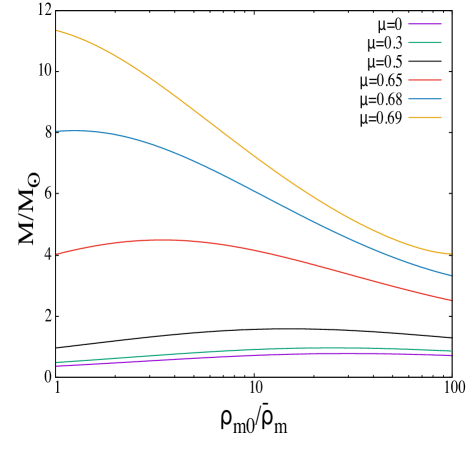
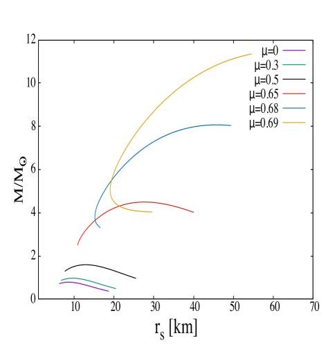
Figure 1: (Left) The ADM mass $M$ (normalized by the solar mass $M_{\odot}$) versus the central mass density $\rho_{m0}$ (normalized by $\bar{\rho}_{m}=1.6749\times 10^{14}$ g cm^-3) for $\beta=0$. We choose the polytropic EOS with $\Gamma=5/3$ and $K=0.018$. Each line corresponds to the plot for several different values of $\mu$ shown in the label. (Right) $M/M_{\odot}$ versus the star radius $r_{s}$ for the same EOS and the values of $\mu$ as those used in the left panel. The central mass density is in the range $1\leq\rho_{m0}/\bar{\rho}_{m}\leq 100$.

As $\mu$ approaches the upper bound (59), i.e., $\mu\simeq 0.7$, the increase of $M$ tends to be significant. Even though $M$ is smaller than $M_{\odot}$ for $\mu=0$, the presence of a large charge density with $\mu=0.69$ can result in the value of $M$ exceeding $10M_{\odot}$ in the region of low matter densities. In the left panel of Fig. 1, we also find that, for $\mu$ close to 0.7, the derivative ${\rm d}M/{\rm d}\rho_{m0}$ is negative for most of $\rho_{m0}$ in the range $\bar{\rho}_{m}\leq\rho_{m0}\leq 100\bar{\rho}_{m}$. For $\mu>1/\sqrt{2}$, our numerical simulations show that gravitationally bounded stars cease to exist. Besides the ADM mass $M$, we compute the proper mass $M_{p}$ defined in Eq. (35) and find that the binding energy $\Delta=M_{p}-M$ is positive for $\mu<1/\sqrt{2}$. As $\mu$ increases toward this upper bound, the ADM mass $M$ tends to approach $M_{p}$ for most of $\rho_{m0}$ chosen in Fig. 1. This supports our claim that the gravitationally bounded stars can exist for $\mu<1/\sqrt{2}$. We note that the above results are consistent with those obtained in Ref. Ray:2003gt in Einstein-Maxwell theory.

IV.3 Scalarized solutions for $\beta<0$

IV.3.1 Existence of scalarized solutions

For the negative scalar-gauge coupling ($\beta<0$), we explore the presence of scalarized solutions with $\phi(r)\neq 0$ besides the GR branch with $\phi(r)=0$. Note that the GR branch corresponds to that discussed in Sec. IV.2. We consider a positive value of $\phi_{0}$ and adopt the polytropic EOS same as used in Sec. IV.2. In the left panel of Fig. 2, we plot an example of the scalarized branch for $\beta=-5$ and $\mu=0.68$ with $\chi=10$ at $r=0$. The field value at $r=0$ is determined to be $\phi_{0}\simeq 0.2208M_{\rm pl}$ to satisfy the boundary condition $\phi_{f}\equiv\phi(\infty)=0$ at spatial infinity. Around $r=0$, the scalar field slowly varies, according to Eq. (53). The variation of $\phi(r)$ tends to be significant around the surface of star ($s\simeq 0.13$). For $r\gg r_{s}$, the scalar field decreases toward 0 with its derivative $\phi^{\prime}(r)$ proportional to $r^{-2}$. The derivative of $A_{t}$ has the dependence ${\rm d}A_{t}/{\rm d}s\propto r^{2}$ for $r\ll r_{s}$ and ${\rm d}A_{t}/{\rm d}s\propto r^{-1}$ for $r\gg r_{s}$. The mass function $m(r)$, which acquires the contributions from $\phi^{\prime}(r)$ and $A_{t}^{\prime}(r)$ even outside the star, approaches the constant value $m(r)\to 1.62$ as $r\to\infty$.

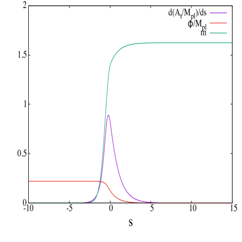
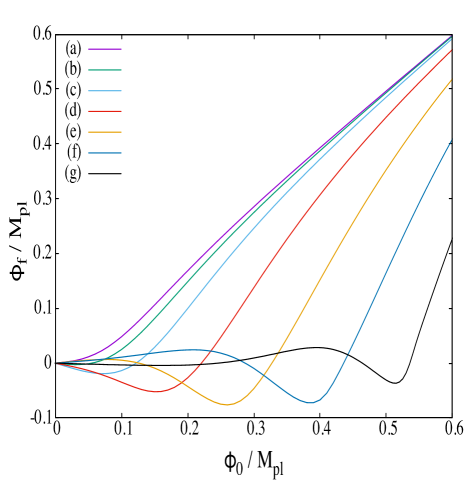
Figure 2: (Left) ${\rm d}(A_{t}/M_{\rm pl})/{\rm d}s$, $\phi/M_{\rm pl}$, and $m$ versus $s=\ln r/\bar{r}$ for $\beta=-5$, $\mu=0.68$, and $\chi_{0}=10$, where $\chi_{0}$ is the value of $\chi$ at $r=0$. The EOS is the same as that used in Fig. 1. The field value $\phi_{0}\simeq 0.2208$ at $r=0$ is chosen to satisfy the boundary condition $\phi_{f}=0$. (Right) The field value $\phi_{f}$ at spatial infinity normalized by $M_{\rm pl}$ versus $\phi_{0}/M_{\rm pl}$ for $\beta=-5$ and $\mu=0.68$ with the same EOS as in the left panel. Each case corresponds to (a) $\chi_{0}=1$, (b) $\chi_{0}=10^{1/5}$, (c) $\chi_{0}=10^{1/2}$, (d) $\chi_{0}=10$, (e) $\chi_{0}=10^{3/2}$, (f) $\chi_{0}=10^{2}$, and (g) $\chi_{0}=10^{5/2}$.

In the right panel of Fig. 2, we show the dependence of $\phi_{f}$ on the change of $\phi_{0}$ for seven different central matter densities, with $\beta=-5$ and $\mu=0.68$. In case (a), there is no nonvanishing value of $\phi_{0}$ leading to $\phi_{f}=0$, so the GR branch $\phi(r)=0$ is the only allowed solution. For $\chi_{0}\gtrsim 1.3$, however, there are intersections of the curve with $\phi_{f}=0$ at a point $\phi_{0}>0$. This is the appearance of a scalarized branch where $\phi(r)$ changes from $\phi_{0}$ (at $r=0$) to $0$ (at $r\to\infty$). The field profile shown in the left panel of Fig. 2 corresponds to case (d) in the right panel, i.e., $\phi_{0}\simeq 0.2208M_{\rm pl}$ at $\phi_{f}=0$.

In cases (b)-(d) the shapes of curves in the $(\phi_{0},\phi_{f})$ plane, which are convex downward with the existence of the region $\phi_{f}<0$, are similar to those for spontaneous scalarization induced by a nonminimal scalar-field coupling with the Ricci scalar Kase:2020yhw . This shows that, for a wide range of central matter densities, the scalar-gauge coupling gives rise to hairy solutions which are expected to be the end points of tachyonic instabilities of the GR branch with $\phi(r)=0$. In order to verify that the new hairy branch is indeed the endpoint of tachyonic instabilities, we need perturbative stability analysis Harada:1998ge and numerical simulations Novak:1998rk for the dynamical evolution toward the scalarized solution.

In cases (e) and (f), there are two intersection points of the theoretical curve with $\phi_{f}=0$. One of them has the property ${\rm d}\phi_{f}/{\rm d}\phi_{0}>0$ around $\phi_{f}=0$, whereas the other has the negative sign of ${\rm d}\phi_{f}/{\rm d}\phi_{0}$. The former corresponds to a 0-node solution where $\phi(r)$ monotonically decreases toward 0 from $r=0$ to $r\to\infty$. The latter is known as a 1-node solution where $\phi(r)$ crosses 0 at finite distance and approaches 0 toward infinity from the side $\phi(r)<0$. For the 1-node solution with ${\rm d}\phi_{f}/{\rm d}\phi_{0}<0$, a positive shift of $\phi_{0}$ leads to a negative shift of $\phi_{f}$, whose property is different from the 0-node solution. Moreover, the 1-node can be regarded as an excited state of solutions, while the 0-node should be in a more stable ground state. For the computations of $M$ and $r_{s}$, we will adopt the values $\phi_{0}\simeq 0.3274M_{\rm pl}$ and $\phi_{0}\simeq 0.4357M_{\rm pl}$ in cases (e) and (f), respectively, both of which correspond to the 0-node solutions.

In case (g), the 2-node solution with ${\rm d}\phi_{f}/{\rm d}\phi_{0}>0$ arises at $\phi_{0}\simeq 0.2457M_{\rm pl}$, besides the 1-node ($\phi_{0}\simeq 0.4639M_{\rm pl}$) and the 0-node ($\phi_{0}\simeq 0.5356M_{\rm pl}$). Since the higher-node solutions should correspond to more excited states of the charged star, it is generally expected that the 0-node corresponds to an endpoint of tachyonic instabilities of the GR branch. For increasing $\chi_{0}$ further, the solutions with additional higher nodes like the 3-node can appear, but this is the region of extremely high matter densities which are out of the configuration of standard relativistic stars. For this reason, we will focus on the matter density in the range $\rho_{m0}\leq 100\bar{\rho}_{m}$ (i.e., $\chi_{0}<68.8$) in the following discussion. In this regime, all the scalarized field profiles with ${\rm d}\phi_{f}/{\rm d}\phi_{0}>0$ at $\phi_{f}=0$ correspond to the 0-node solutions.

IV.3.2 Properties of scalarized solutions

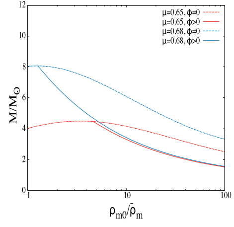
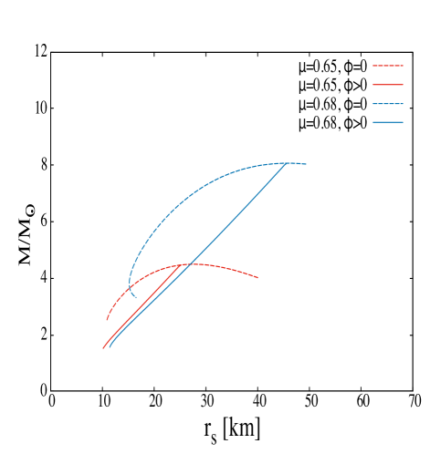
Figure 3: $M/M_{\odot}$ versus $\rho_{m0}/\bar{\rho}_{m}$ (left) and $M/M_{\odot}$ versus $r_{s}$ (right) for $\beta=-5$. The red solid and blue solid lines correspond to the scalarized branch ($\phi(r)\neq 0$) with $\mu=0.65$ and $\mu=0.68$, respectively. The red dashed and blue dashed lines represent the GR branch ($\phi(r)=0$) for $\mu=0.65$ and $\mu=0.68$, respectively. The EOS is the same as that used in Fig. 1. In the right panel, the central mass density is in the range $\bar{\rho}_{m}\leq\rho_{m0}\leq 100\bar{\rho}_{m}$.

In Fig. 3, we plot $M/M_{\odot}$ versus $\rho_{m0}/\bar{\rho}_{m}$ (left) and $M/M_{\odot}$ versus $r_{s}$ (right) with the coupling $\beta=-5$ for two different values of $\mu$. We note that all the nontrivial solutions shown in Fig. 3 are the 0-node solutions. When $\mu=0.68$, the hairy solutions with $\phi(r)\neq 0$ start to appear for the central matter density $\rho_{m0}$ larger than $1.3\bar{\rho}_{m}$. In this regime, the deviations of $M$ and $r_{s}$ from those in the GR branch can be seen in Fig. 3. The negative coupling $\beta<0$ with $\phi(r)\neq 0$ suppresses the Coulomb force $e^{\beta\phi_{0}^{2}/M_{\rm pl}^{2}}\rho_{c0}^{2}r^{2}/6$ in Eq. (57) around $r=0$. The faster decrease of $P_{m}$ induced by the scalarized branch results in smaller values of $r_{s}$ and $M$ relative to those in the GR branch. Unlike spontaneous scalarization of nonminimally coupled scalar-tensor theories Damour:1993hw ; Damour2 , the scalar-gauge coupling gives rise to a charged star configuration with the decreased values of $M$. In the right panel of Fig. 3, we observe that the ADM mass of the scalarized solution is almost proportional to $r_{s}$.

When $\mu=0.65$ and $\beta=-5$, the scalarized branch starts to appear for $\rho_{m0}\gtrsim 4.5\bar{\rho}_{m}$. The ADM masses of the GR branch exhibit large differences between $\mu=0.65$ and $\mu=0.68$, but the corresponding masses and radii of scalarized solutions are not much different between these two values of $\mu$. This can be regarded as the consequence of stabilizations of solutions induced by the negative scalar-gauge coupling $\beta$, in a way that the slight change of $\mu$ results in only small modifications to $M$ and $r_{s}$. We numerically find that, for $\beta=-5$ and $\mu\lesssim 0.5$, the scalarized branch does not exist at least in the range $\rho_{m0}\leq 100\bar{\rho}_{m}$. For $\mu>1/\sqrt{2}$, the negative coupling with $\beta=-5$ hardly gives rise to scalarized solutions with $P_{m}$ decreasing toward the surface of star. This is related to the fact that the field value $\phi_{0}$ at $r=0$ does not exceed the order of $M_{\rm pl}$, so the Coulomb force $e^{\beta\phi_{0}^{2}/M_{\rm pl}^{2}}\rho_{c0}^{2}r^{2}/6$ is not significantly suppressed compared to that of the GR branch. In summary, for $\beta=-5$ and $\rho_{m0}\lesssim 100\bar{\rho}_{m}$, the scalarized charged star solutions exist in the range $0.5\lesssim\mu\lesssim 0.7$.

We have also numerically confirmed the existence of 0-node scalarized solutions by considering different values of $\beta$ and $\mu$. When $\beta=-{\cal O}(0.1)$, we find that the scalarized solutions can be present only for high values of $\rho_{m0}~{}(\gtrsim{\cal O}(10)\bar{\rho}_{m})$ with $\mu$ close to $1/\sqrt{2}$. For $\beta=-{\cal O}(1)$, the scalarized solutions exist for $0.45\lesssim\mu\lesssim 0.7$ in the broader range of $\rho_{m0}$. As $\mu$ increases toward the value $1/\sqrt{2}$, the ADM mass $M$ is subject to stronger decrease by spontaneous scalarization relative to that in the GR branch. When $|\beta|$ exceeds the order 10, the scalar field does not change much inside the star, see Eq. (53). In such cases, there is a tendency that the scalarized solutions disappear especially for the values of $\mu$ much less than 0.7.

IV.4 Implications for spontanenous scalarization of charged stars

The results explained above show that, for $\beta=-{\cal O}(1)$ and $0.45\lesssim\mu\lesssim 0.7$, the GR branch can undergo spontaneous scalarization toward the nonvanishing and nontrivial scalar field solution. The masses and radii of the scalarized branch are smaller than those of the GR branch as a result of the suppressed Coulomb force.

Without performing detailed numerical simulations about the process of spontaneous scalarization, we can speculate to some extent how the transition from the GR solution to the scalarized branch proceeds. For $\mu=0.65$ and $\mu=0.68$ shown in Fig. 3, the 0-node branch is smoothly connected to the GR branch in low density regimes, showing that the scalarized solution arises as the consequence of continuous phase transition from the GR solution. Fig. 3 also indicates that, for $\beta=-5$, the bifurcation point of the 0-node branch from the GR branch is located in the vicinity of the maximal star mass in GR. Hence the bifurcation to the 0-node solution occurs around the maximum mass of gravitationally bounded charged stars in GR.

For a fixed value of $\mu$, the increase of $|\beta|$ within $5\lesssim|\beta|\lesssim 10$ shifts bifurcation points of the 0-node branch toward the regime of smaller densities (larger radii) of the star. In particular, for $\mu=0.68$, the bifurcation point is shifted to the region $\rho_{m0}\lesssim{\bar{\rho}}_{m}$. Thus, spontaneous scalarization to 0-node solutions can occur for a wider range of $\rho_{m0}$. In the presence of a scalar-gauge coupling, tachyonic instabilities excite the scalar field inside the charged GR star and transfer the energies of matter and electric field to the scalar field. A part of the energy of this system would be radiated away via scalar radiation, which reduces the star mass and makes the 0-node scalarized star perturbatively more stable.

V Conclusions

In Einstein-Maxwell-scalar theories, we have studied the possibility for the occurrence of spontaneous scalarization of charged stars. Such theories can be represented by the explicit action (1) with Eqs. (2)-(4) containing the scalar-gauge coupling $-\alpha(\phi)F_{\mu\nu}F^{\mu\nu}/4$ and the matter and charge currents as a generalization of the Schtuz-Sorkin Lagrangian. In Sec. II, we have derived all the field equations of motion in the covariant form and shown that the perfect-fluid energy momentum tensor $T_{\mu\nu}^{(m)}$ obeys the continuity Eq. (19) with the appearance of a Coulomb force on its right hand side.

On the static and spherically symmetric spacetime given by the line element (24), the background equations of motion are of the forms (26)-(30). The field-dependent coupling $\alpha(\phi)$ in Eq. (27) allows the existence of a nonvanishing and nontrivial scalar field profile both inside and outside the star. This affects the gauge-field derivative $A_{t}^{\prime}$ through Eq. (26). Then, the nontrivial $A_{t}^{\prime}$ gives rise to a modified Coulomb force which changes the force balance inside the charged star, so that its mass $M$ and radius $r_{s}$ are generally subject to modifications.

In Sec. IV, we showed that the necessary conditions for spontaneous scalarization to occur are characterized by Eq. (48), which leads to the generic form of the coupling function (49). One of the examples for this realization is the coupling $\alpha(\phi)=\exp(-\beta\phi^{2}/M_{\rm pl}^{2})$ with $\beta<0$. For negative $\beta$, besides the GR branch with $\phi(r)=0$, there exists a scalarized branch where the scalar field profile is given by Eq. (53) for $r\ll r_{s}$ and Eq. (62) for $r\gg r_{s}$. As the ratio $\mu=M_{\rm pl}\rho_{c}/\rho_{m}$ increases toward the upper limit $1/\sqrt{2}$, there are significant enhancement of $M$ and $r_{s}$ in the GR branch induced by a large Coulomb force. For $\beta=-{\cal O}(1)$ and $\rho_{m0}\leq 100\bar{\rho}_{m}$, we numerically confirmed the existence of 0-node scalarized solutions where $\phi(r)$ monotonically decreases from a positive value $\phi_{0}$ (at $r=0$) toward the asymptotic value 0 at spatial infinity. The scalar-gauge coupling with $\beta<0$ effectively reduces the Coulomb force, which results in faster decrease of $P_{m}(r)$. As we observe in Fig. 3, the masses and radii of stars for the scaralized branch are smaller than those of the GR branch. For this scaralized solution, the modifications to $M$ and $r_{s}$ induced by a small change of $\mu$ around $\mu=0.7$ are much less significant in comparison to those of the GR branch.

The appearance of scalarized solutions depends on the central matter density $\rho_{m0}$. As $\rho_{m0}$ increases, the scalar-field profiles higher than the 0-node start to appear, see the right panel of Fig. 2. Since these higher-node solutions correspond to excited states of the charged star, we picked up the 0-node solution as a most stable ground state of the scalarized branch for the polytropic EOS with $\rho_{m0}\leq 100\bar{\rho}_{m}$. We found that, for $\beta=-{\cal O}(1)$ and $0.45\lesssim\mu\lesssim 0.7$, the scalarized (0-node) solutions can exist for a wide range of $\rho_{m0}$. In this regime of $\mu$, the charged GR star with a large Coulomb force should undergo spontaneous scalarization toward the scalarized branch with smaller values of $M$ and $r_{s}$. This property should also hold for other EOSs because the Coulomb force $e^{\beta\phi_{0}^{2}/M_{\rm pl}^{2}}\rho_{c0}^{2}r^{2}/6$ appearing in the iterative solution (57) of $P_{m}(r)$ is generally suppressed for the scalarized branch with negative $\beta$.

It will be of interest to study the stability of our new scalarized solutions against perturbations in the odd- and even-parity sectors. The analysis can be done in the similar way to that performed for relativistic stars in nonminimally coupled scalar-tensor theories Kase:2020qvz . We leave this issue for a future work.

References

- (1) B. P. Abbott et al. [LIGO Scientific and Virgo Collaborations], Phys. Rev. Lett. 116, 061102 (2016) [arXiv:1602.03837 [gr-qc]].
- (2) B. P. Abbott et al. [LIGO Scientific and Virgo Collaborations], Phys. Rev. Lett. 119, 161101 (2017) [arXiv:1710.05832 [gr-qc]].
- (3) E. Berti et al., Class. Quant. Grav. 32, 243001 (2015) [arXiv:1501.07274 [gr-qc]].
- (4) L. Barack et al., Class. Quant. Grav. 36, 143001 (2019) [arXiv:1806.05195 [gr-qc]].
- (5) E. Berti, K. Yagi and N. Yunes, Gen. Rel. Grav. 50, no.4, 46 (2018) [arXiv:1801.03208 [gr-qc]].
- (6) T. Damour and G. Esposito-Farese, Phys. Rev. Lett. 70, 2220-2223 (1993).
- (7) T. Damour and G. Esposito-Farese, Phys. Rev. D 54, 1474 (1996) [gr-qc/9602056].
- (8) P. Kanti, N. E. Mavromatos, J. Rizos, K. Tamvakis and E. Winstanley, Phys. Rev. D 54, 5049-5058 (1996) [arXiv:hep-th/9511071 [hep-th]].
- (9) S. O. Alexeev and M. V. Pomazanov, Phys. Rev. D 55, 2110-2118 (1997) [arXiv:hep-th/9605106 [hep-th]].
- (10) A. Cooney, S. DeDeo and D. Psaltis, Phys. Rev. D 82, 064033 (2010) [arXiv:0910.5480 [astro-ph.HE]].
- (11) A. S. Arapoglu, C. Deliduman and K. Y. Eksi, JCAP 1107, 020 (2011) [arXiv:1003.3179 [gr-qc]].
- (12) M. Rinaldi, Phys. Rev. D 86, 084048 (2012) [arXiv:1208.0103 [gr-qc]].
- (13) M. Minamitsuji, Phys. Rev. D 89, 064017 (2014) [arXiv:1312.3759 [gr-qc]].
- (14) T. P. Sotiriou and S. Y. Zhou, Phys. Rev. Lett. 112, 251102 (2014) [arXiv:1312.3622 [gr-qc]].
- (15) T. P. Sotiriou and S. Y. Zhou, Phys. Rev. D 90, 124063 (2014) [arXiv:1408.1698 [gr-qc]].
- (16) S. S. Yazadjiev, D. D. Doneva, K. D. Kokkotas and K. V. Staykov, JCAP 1406, 003 (2014) [arXiv:1402.4469 [gr-qc]].
- (17) E. Babichev, C. Charmousis and A. Lehébel, JCAP 1704, 027 (2017) [arXiv:1702.01938 [gr-qc]].
- (18) E. Babichev and C. Charmousis, JHEP 1408, 106 (2014) [arXiv:1312.3204 [gr-qc]].
- (19) T. Kobayashi and N. Tanahashi, PTEP 2014, 073E02 (2014) [arXiv:1403.4364 [gr-qc]].
- (20) S. S. Yazadjiev, D. D. Doneva and D. Popchev, Phys. Rev. D 93, 084038 (2016) [arXiv:1602.04766 [gr-qc]].
- (21) E. Babichev, C. Charmousis, A. Lehébel and T. Moskalets, JCAP 1609, 011 (2016) [arXiv:1605.07438 [gr-qc]].
- (22) J. Chagoya, G. Niz and G. Tasinato, Class. Quant. Grav. 34 (2017) no.16, 165002 [arXiv:1703.09555 [gr-qc]].
- (23) M. Minamitsuji, Phys. Rev. D 94, 084039 (2016) [arXiv:1607.06278 [gr-qc]].
- (24) L. Heisenberg, R. Kase, M. Minamitsuji and S. Tsujikawa, Phys. Rev. D 96, 084049 (2017) [arXiv:1705.09662 [gr-qc]].
- (25) L. Heisenberg, R. Kase, M. Minamitsuji and S. Tsujikawa, JCAP 1708, 024 (2017) [arXiv:1706.05115 [gr-qc]].
- (26) Z. Y. Fan, JHEP 1609, 039 (2016) [arXiv:1606.00684 [hep-th]].
- (27) A. Cisterna, M. Hassaine, J. Oliva and M. Rinaldi, Phys. Rev. D 94, 104039 (2016). [arXiv:1609.03430 [gr-qc]].
- (28) E. Babichev, C. Charmousis and M. Hassaine, JHEP 1705, 114 (2017) [arXiv:1703.07676 [gr-qc]].
- (29) R. Kase, M. Minamitsuji and S. Tsujikawa, Phys. Rev. D 97, 084009 (2018) [arXiv:1711.08713 [gr-qc]].
- (30) R. Kase, M. Minamitsuji and S. Tsujikawa, Phys. Lett. B 782, 541-550 (2018) [arXiv:1803.06335 [gr-qc]].
- (31) R. Kase and S. Tsujikawa, JCAP 09, 054 (2019) [arXiv:1906.08954 [gr-qc]].
- (32) T. Kobayashi and T. Hiramatsu, Phys. Rev. D 97, 104012 (2018). [arXiv:1803.10510 [gr-qc]].
- (33) J. Ben Achour and H. Liu, Phys. Rev. D 99, 064042 (2019) [arXiv:1811.05369 [gr-qc]].
- (34) H. Motohashi and M. Minamitsuji, Phys. Rev. D 99, 064040 (2019). [arXiv:1901.04658 [gr-qc]].
- (35) M. Minamitsuji and J. Edholm, Phys. Rev. D 101, 044034 (2020). [arXiv:1912.01744 [gr-qc]].
- (36) T. Harada, Phys. Rev. D 57, 4802 (1998) [gr-qc/9801049].
- (37) J. Novak, Phys. Rev. D 58, 064019 (1998) [gr-qc/9806022].
- (38) H. O. Silva, C. F. B. Macedo, E. Berti and L. C. B. Crispino, Class. Quant. Grav. 32, 145008 (2015) [arXiv:1411.6286 [gr-qc]].
- (39) R. Kase, R. Kimura, S. Sato and S. Tsujikawa, Phys. Rev. D 102, 084037 (2020) [arXiv:2007.09864 [gr-qc]].
- (40) H. Sotani and K. D. Kokkotas, Phys. Rev. D 70, 084026 (2004) [arXiv:gr-qc/0409066 [gr-qc]].
- (41) P. C. C. Freire et al., Mon. Not. Roy. Astron. Soc. 423, 3328 (2012) [arXiv:1205.1450 [astro-ph.GA]].
- (42) H. Sotani, Phys. Rev. D 89, 064031 (2014) [arXiv:1402.5699 [astro-ph.HE]].
- (43) G. Pappas and T. P. Sotiriou, Mon. Not. Roy. Astron. Soc. 453, 2862-2876 (2015) [arXiv:1505.02882 [gr-qc]].
- (44) H. Sotani, Phys. Rev. D 86, 124036 (2012) [arXiv:1211.6986 [astro-ph.HE]].
- (45) D. D. Doneva, S. S. Yazadjiev, N. Stergioulas and K. D. Kokkotas, Phys. Rev. D 88, 084060 (2013) [arXiv:1309.0605 [gr-qc]].
- (46) D. D. Doneva, S. S. Yazadjiev, K. V. Staykov and K. D. Kokkotas, Phys. Rev. D 90, 104021 (2014) [arXiv:1408.1641 [gr-qc]].
- (47) P. Pani and E. Berti, Phys. Rev. D 90, 024025 (2014) [arXiv:1405.4547 [gr-qc]].
- (48) D. D. Doneva, S. S. Yazadjiev, N. Stergioulas, K. D. Kokkotas and T. M. Athanasiadis, Phys. Rev. D 90, 044004 (2014) [arXiv:1405.6976 [astro-ph.HE]].
- (49) M. Minamitsuji and H. O. Silva, Phys. Rev. D 93, 124041 (2016) [arXiv:1604.07742 [gr-qc]].
- (50) L. Annulli, V. Cardoso and L. Gualtieri, Phys. Rev. D 99, 044038 (2019) [arXiv:1901.02461 [gr-qc]].
- (51) F. M. Ramazanoğlu, Phys. Rev. D 99, 084015 (2019) [arXiv:1901.10009 [gr-qc]].
- (52) R. Kase, M. Minamitsuji and S. Tsujikawa, Phys. Rev. D 102, 024067 (2020) [arXiv:2001.10701 [gr-qc]].
- (53) M. Minamitsuji, Phys. Rev. D 101, 104044 (2020) [arXiv:2003.11885 [gr-qc]].
- (54) F. M. Ramazanoğlu, Phys. Rev. D 96, 064009 (2017). [arXiv:1706.01056 [gr-qc]].
- (55) F. M. Ramazanoğlu, Phys. Rev. D 98, 044011(2018) [erratum: Phys. Rev. D 100, 029903 (2019)] [arXiv:1804.00594 [gr-qc]].
- (56) M. Minamitsuji, Phys. Rev. D 102, 044048 (2020) [arXiv:2008.12758 [gr-qc]].
- (57) D. D. Doneva and S. S. Yazadjiev, Phys. Rev. Lett. 120, 131103 (2018) [arXiv:1711.01187 [gr-qc]].
- (58) H. O. Silva, J. Sakstein, L. Gualtieri, T. P. Sotiriou and E. Berti, Phys. Rev. Lett. 120, 131104 (2018) [arXiv:1711.02080 [gr-qc]].
- (59) H. O. Silva, C. F. B. Macedo, T. P. Sotiriou, L. Gualtieri, J. Sakstein and E. Berti, Phys. Rev. D 99, 064011 (2019) [arXiv:1812.05590 [gr-qc]].
- (60) G. Antoniou, A. Bakopoulos and P. Kanti, Phys. Rev. Lett. 120, 131102 (2018) [arXiv:1711.03390 [hep-th]].
- (61) G. Antoniou, A. Bakopoulos and P. Kanti, Phys. Rev. D 97, 084037 (2018) [arXiv:1711.07431 [hep-th]].
- (62) M. Minamitsuji and T. Ikeda, Phys. Rev. D 99, 044017 (2019) [arXiv:1812.03551 [gr-qc]].
- (63) P. V. P. Cunha, C. A. R. Herdeiro and E. Radu, Phys. Rev. Lett. 123, 011101 (2019) [arXiv:1904.09997 [gr-qc]].
- (64) A. Dima, E. Barausse, N. Franchini and T. P. Sotiriou, Phys. Rev. Lett. 125, 231101 (2020) [arXiv:2006.03095 [gr-qc]].
- (65) S. Hod, Phys. Rev. D 102, no.8, 084060 (2020) [arXiv:2006.09399 [gr-qc]].
- (66) C. A. R. Herdeiro, E. Radu, H. O. Silva, T. P. Sotiriou and N. Yunes, Phys. Rev. Lett. 126, 011103 (2021) [arXiv:2009.03904 [gr-qc]].
- (67) E. Berti, L. G. Collodel, B. Kleihaus and J. Kunz, Phys. Rev. Lett. 126, 011104 (2021) [arXiv:2009.03905 [gr-qc]].
- (68) D. D. Doneva and S. S. Yazadjiev, Phys. Rev. D 103 (2021) no.6, 064024 [arXiv:2101.03514 [gr-qc]].
- (69) Y. X. Gao, Y. Huang and D. J. Liu, Phys. Rev. D 99, 044020 (2019) [arXiv:1808.01433 [gr-qc]].
- (70) Y. S. Myung and D. C. Zou, Phys. Lett. B 814, 136081 (2021) [arXiv:2012.02375 [gr-qc]].
- (71) D. D. Doneva and S. S. Yazadjiev, Phys. Rev. D 103, 083007 (2021) [arXiv:2102.03940 [gr-qc]].
- (72) I. Z. Stefanov, S. S. Yazadjiev and M. D. Todorov, Mod. Phys. Lett. A 23, 2915 (2008) [arXiv:0708.4141 [gr-qc]].
- (73) C. A. R. Herdeiro, E. Radu, N. Sanchis-Gual and J. A. Font, Phys. Rev. Lett. 121, 101102 (2018) [arXiv:1806.05190 [gr-qc]].
- (74) Y. S. Myung and D. C. Zou, Eur. Phys. J. C 79, no.3, 273 (2019) [arXiv:1808.02609 [gr-qc]].
- (75) P. G. S. Fernandes, C. A. R. Herdeiro, A. M. Pombo, E. Radu and N. Sanchis-Gual, Class. Quant. Grav. 36, 134002 (2019) [arXiv:1902.05079 [gr-qc]].
- (76) Y. Brihaye and B. Hartmann, Phys. Lett. B 792, 244-250 (2019) [arXiv:1902.05760 [gr-qc]].
- (77) Y. S. Myung and D. C. Zou, Eur. Phys. J. C 79, no.8, 641 (2019) [arXiv:1904.09864 [gr-qc]].
- (78) P. G. S. Fernandes, C. A. R. Herdeiro, A. M. Pombo, E. Radu and N. Sanchis-Gual, Phys. Rev. D 100, 084045 (2019) [arXiv:1908.00037 [gr-qc]].
- (79) T. Ikeda, T. Nakamura and M. Minamitsuji, Phys. Rev. D 100, 104014 (2019) [arXiv:1908.09394 [gr-qc]].
- (80) S. Hod, Phys. Lett. B 798, 135025 (2019) [arXiv:2002.01948 [gr-qc]].
- (81) G. W. Gibbons and K. i. Maeda, Nucl. Phys. B 298, 741-775 (1988).
- (82) D. Garfinkle, G. T. Horowitz and A. Strominger, Phys. Rev. D 43, 3140 (1991) [erratum: Phys. Rev. D 45, 3888 (1992)].
- (83) S. Mignemi and N. R. Stewart, Phys. Rev. D 47, 5259-5269 (1993) [arXiv:hep-th/9212146 [hep-th]].
- (84) T. Torii, H. Yajima and K. i. Maeda, Phys. Rev. D 55, 739-753 (1997) [arXiv:gr-qc/9606034 [gr-qc]].
- (85) C. A. R. Herdeiro, T. Ikeda, M. Minamitsuji, T. Nakamura and E. Radu, Phys. Rev. D 103, no.4, 044019 (2021) [arXiv:2009.06971 [gr-qc]].
- (86) S. Ray, A. L. Espindola, M. Malheiro, J. P. S. Lemos and V. T. Zanchin, Phys. Rev. D 68, 084004 (2003) [arXiv:astro-ph/0307262 [astro-ph]].
- (87) J. D. Bekenstein, Phys. Rev. D 4, 2185-2190 (1971).
- (88) F. de Felice, S. m. Liu and Y. q. Yu, Class. Quant. Grav. 16, 2669-2680 (1999) [arXiv:gr-qc/9905099 [gr-qc]].
- (89) P. Anninos and T. Rothman, Phys. Rev. D 65, 024003 (2002) [arXiv:gr-qc/0108082 [gr-qc]].
- (90) B. F. Schutz and R. Sorkin, Annals Phys. 107, 1 (1977).
- (91) J. D. Brown, Class. Quant. Grav. 10, 1579 (1993) [gr-qc/9304026].
- (92) A. De Felice, J. M. Gerard and T. Suyama, Phys. Rev. D 81, 063527 (2010) [arXiv:0908.3439 [gr-qc]].
- (93) R. Kase and S. Tsujikawa, JCAP 11, 032 (2020) [arXiv:2005.13809 [gr-qc]].
- (94) R. Kase and S. Tsujikawa, JCAP 01, 008 (2021) [arXiv:2008.13350 [gr-qc]].