Eco-Driving of Connected and Autonomous Vehicles with Sequence-to-Sequence Prediction of Target Vehicle Velocity

Abstract

The Eco-Driving control problem seeks to perform fuel efficient speed planning for a Connected and Autonomous Vehicle (CAV) that can exploit information available from advanced mapping, and from Vehicle-to-Everything (V2X) communication. The ability of an Eco-Driving strategy to adapt in real time to variable traffic scenarios where surrounding vehicles can be either connected or unconnected is critical for further development and deployment of this technology in the transportation sector.

In this work, the Eco-Driving strategy, formulated as a receding-horizon optimal control problem, is integrated with a target vehicle speed prediction model and solved via Dynamic Programming (DP) to determine the optimal speed trajectory in the presence of a human-driven target vehicle. An encoder-decoder architecture analyzes the patterns in the target vehicle velocity recorded over a historic window using a Gated-Recurrent-Unit (GRU) based encoder and generates an estimate of the future velocity trajectory using the GRU based decoder. A sensitivity study is done to analyze the effect of the historical and prediction windows on the accuracy of the velocity predictor. The proposed Eco-Driving controller is evaluated through microscopic simulations using a traffic simulator.

1 Introduction

The recent advancements in Connected and Automated Vehicles (CAVs) technologies have the potential to increase safety, driving comfort as well as fuel economy, by exploiting information on driving conditions ahead that become available via advanced navigation systems, Vehicle-to-Vehicle (V2V) and Vehicle-to-Infrastructure (V2I) communication (Guanetti et al. (2018)). Intuitively, the availability of such technologies could be exploited in a predictive controller to plan a speed trajectory that minimizes unnecessary acceleration and braking events, thereby improving driver comfort and fuel-efficiency (Xu and Peng (2018)). Furthermore, information on future driving conditions could enhance energy efficiency gains in electrified powertrain, by optimally scheduling the use of the electric motors and onboard battery pack (Guzzella et al. (2007)).

In this scenario, Eco-Driving aims at exploiting information on future driving conditions to optimize speed planning and powertrain control for improving the fuel efficiency between an origin and destination. However, Eco-Driving algorithms pose challenges for the design of a predictive (look-ahead) controller, especially in presence of uncertain traffic environment (Alam and McNabola (2014)). Another limitation of the existing literature in Eco-Driving is that the problem of speed trajectory optimization and powertrain control is often treated as two decentralized problems to reduce the computational complexity. In this case, the speed trajectory prediction of the target vehicle is incorporated in the speed planning problem, and the resulting ego vehicle speed trajectory is utilized as an external input for the sub-problem of powertrain control optimization (Firoozi et al. (2018)).

For real-world implementation of Eco-Driving controls, it is crucial to predict the presence of target vehicles as additional dynamic states, and incorporate them into the trajectory planning process. While some work has been done to incorporate a velocity prediction for a fully or partially connected target vehicle (see for instance Sun et al. (2014); Kamal et al. (2015)), however such assumptions might not be realistic in a partially connected environment where the ego vehicle might have access to only the current value of the target vehicle velocity.

In addition, forecasting the speed trajectory of a human-driven vehicle (no automation) in urban driving is a very difficult task, as the vehicle’s maneuvers may by affected by various dynamic factors, for instance traffic light Signal Phasing and Timing (SPaT), driver’s experience, weather, etc. Earlier studies have assumed simple but unrealistic speed trajectories, such as constant speed and constant acceleration when no information is available (for example, Lefèvre et al. (2014)). Auto-regressive models proved to be more realistic when compared to the constant acceleration case, but these prediction methods induce large errors in a prediction horizon, ultimately degrading the controller performance (Hyeon et al. (2019)). More sophisticated model-based car-following models have been proposed by Gupta et al. (2019); Rajakumar Deshpande et al. (2020), however these models require the look-ahead driving information of the human-driven target vehicle within a Line-of-Sight (LoS), which may not be available to the ego vehicle. Data-driven methods such as Long-Short-Term-Memory (LSTM) have been recently studied for forecasting speed trajectories, since they have the ability of predicting highly non-linear time-series with minimal input information (Altché and de La Fortelle (2017)). Although LSTM have proven to have high accuracy, they generally require large training time and are ideal for long-term prediction (Altché and de La Fortelle (2017)).

This work proposes a unified Eco-Driving framework that performs co-optimization of vehicle velocity and powertrain control, as shown in Fig. 1. The proposed architecture acquires various information from multiple data resources, including route information (speed limits, road grade, position of route markers such as traffic lights and stops signs) from an advanced navigation system, SPaT information from a Dedicated Short Range Communication (DSRC) unit, and target vehicle velocity data from V2V communication or on-board detection system (comprises of radar and camera unit). A simpler but faster variant of LSTM namely Gated Recurrent Unit (GRU) is used to build an Encoder-Decoder (ED) network that provides an estimate of the future target vehicle speed trajectory. Existing literature has shown that GRU’s are faster, compact and ideal for short-term predictions (Gao et al. (2020)). The speed predictor is integrated into the Eco-Driving controller to estimate the future speed trajectory of the target vehicle. The optimization is performed in two stages, including a long-term optimization that computes a base policy utilizing the route information from the navigation system available over the entire itinerary, and a receding-horizon optimization that incorporates V2X communications and periodically performs the co-optimization of vehicle velocity and powertrain control over a short horizon. The proposed Eco-Driving controller is evaluated through microscopic simulations.

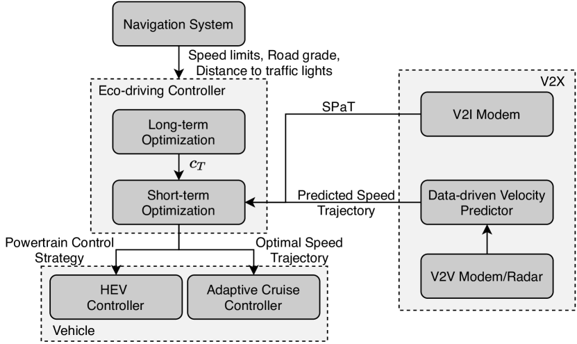
Figure 1: Control architecture of proposed Eco-Driving controller exploiting V2X technology in presence of partially connected, human-driven target vehicle.

2 Mild Hybrid Electric Vehicle Model

A forward-looking parallel mild-Hybrid Electric Vehicle (HEV) is considered, as shown in Olin et al. (2019). A P0 HEV powertrain with a Belted Starter Generator (BSG) performs torque assist, regenerative braking and start-stop functions over real-world routes. The BSG is connected to the crankshaft of a 1.8L turbocharged gasoline engine and a 48V battery pack.

Fig. 2 illustrates the inputs to the Vehicle Dynamics and Powertrain (VD&PT) model, obtained from a simplified model of the Engine Control Module (ECM) that contains the essential functions to convert the driver’s input (pedal position) to torque commands. The outputs of the ECM, the desired BSG torque ($T^{des}_{bsg}$) and desired engine torque ($T^{des}_{eng}$) are obtained from a production level torque split strategy, which is used as the baseline for fuel economy evaluation.

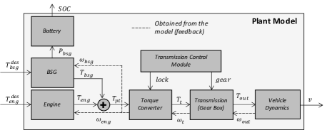
Figure 2: Block Diagram of 48V P0 Mild-Hybrid Drivetrain.

The simulator contains low-frequency dynamic models of the powertrain and longitudinal vehicle dynamics. The battery is modeled as a zero-th order equivalent circuit, from which the battery State-of-Charge (SoC) is calculated; the vehicle longitudinal dynamics are described by the road load equation (Guzzella et al. (2007)). Quasi-static models are developed for the engine (fuel and friction maps), BSG, torque converter and transmission (efficiency maps). The model was validated on chassis dynamometer data. Fig. 3 shows a verification over the FTP drive cycle, where the vehicle velocity, battery SoC ($\xi$) and fuel consumption are compared against test data. Despite small mismatches in the battery SoC, attributed to simplification of the 12V electrical system, the fuel consumption is predicted with cumulative error less than 4%, which is sufficiently accurate for the intended use.

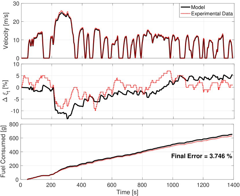
Figure 3: Validation of Vehicle Velocity, SoC ($\xi_{t}$) and Fuel Consumed over FTP Cycle.

3 Target Vehicle Velocity Prediction

Prediction of target vehicle velocity is essential for efficiently applying Eco-Driving in urban traffic conditions. Most of the work published to date assume that the target vehicle is either connected to the infrastructure or to the ego vehicle. Since this assumption is rather limiting, the prediction here developed considers that only the current value of the target vehicle velocity is available at each time step. This represents the most general case of an ego vehicle equipped with an object detection system.

The short term planning of a typical human driver with respect to traffic conditions is generally represented as a time-varying, nonlinear time-series in terms of speed and acceleration (Toledo et al. (2007); Gupta et al. (2019)). Despite the flexibility and power of Deep Neural Networks (DNNs), they are not ideal for sequences, since they require the dimensionality of input and output to be known and fixed (Sutskever et al. (2014)). In this work, the time-dependent nature of the driver behavior is captured by using sequence-to-sequence modeling via a Gated Recurrent Unit Encoder-Decoder.

3.1 Gated Recurrent Unit Encoder-Decoder Architecture

The concept of Gated Recurrent Unit (GRU) was originally proposed by Chung et al. (2014) to overcome the vanishing gradient problem in Vanilla RNNs (Pascanu et al. (2013)) and make each recurrent unit adaptively capture temporal dependencies of sequential data. A GRU network has two gating units: a reset gate $r_{t}$ and an update gate $z_{t}$ that modulate the flow of information inside the unit. The reset gate determines how much of the past information to forget, and the update gate determines how much of the past information needs to be passed along to the future. Even though GRUs do not explicitly contain separate memory cells as in LSTM (Hochreiter and Schmidhuber (1997)), the memory is introduced in the network by the hidden state vector $h_{t}$, which is unique for each input sequence. This makes the GRU relatively fast and compact, suitable for short-term predictions (Gao et al. (2020)).

In this work, a GRU-Encoder-Decoder (GRU-ED) architecture has been used to perform sequence-to-sequence prediction of the target vehicle velocity. In literature, GRU-ED has been extensively used in machine translation tasks (Cho et al. (2014)). GRU-ED is a sequentially connected 3-layer arrangement comprising of an encoder, hidden and decoder layer, as shown in Fig. 4. The encoder layer contains GRU cells that read input sequences one time step at a time to obtain a large fixed-dimensional encoder vector that intrinsically learns the representation in the input sequence. The encoded vector is then fed as input to another sequence of GRU cells contained in the Decoder layer that generates the predicted sequence.

Given an input sequence, $\mathrm{X}=(x_{1},x_{2},\cdots,x_{t})$, where $x_{i}\in\mathbb{R}^{d}$ and $d$ is the feature length of each time step, the GRU encoder computes the sequence of hidden state: $h_{1},h_{2},\cdots,h_{t}$ (Fig. 4) using the equations (Zhang et al. (2017)):

$$z_{t} =\sigma(W_{xz}x_{t}+U_{hz}h_{t-1})$$ (1a)

$$r_{t} =\sigma(W_{xr}x_{t}+U_{hr}h_{t-1})$$ (1b)

$$\tilde{h}_{t} =\tanh\left(W_{xh}x_{t}+U_{rh}(r_{t}\otimes h_{t-1})\right)$$ (1c)

$$h_{t} =(1-z_{t})\otimes h_{t-1}+z_{t}\otimes\tilde{h}_{t}$$ (1d)

where $\sigma$ is the sigmoid function and $\otimes$ is an element-wise multiplication operator; $z_{t},r_{t},\tilde{h}_{t}$ are the update gate, reset gate and candidate activation respectively. $W_{xz},W_{xr},W_{xh},U_{hz},U_{hr},U_{rh}$ are related weight matrices. The decoder then similarly predicts an output sequence $\mathrm{Y}=(\hat{y}_{t+1},\hat{y}_{t+2},\cdots,\hat{y}_{t+T})$, where $\hat{y}_{i}\in\mathbb{R}$ is the predicted velocity.

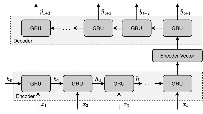
Figure 4: Block Diagram of GRU-ED Architecture.

3.2 Driving Features

The crucial step in developing a vehicle speed prediction model is the selection of a set of input features that are representative of real-world driving. In this work, the input features were selected to be easily measured from ego vehicle’s on-board detection system, without requiring the target vehicle to broadcast its position and velocity. However, it is assumed that V2I communication exists, and more specifically that signalized intersections can broadcast SPaT messages to the ego vehicle within a predetermined transmission range. The longitudinal motion of any vehicle on a straight and flat road over the next time step $\Delta t$ can be determined by the velocity $v_{t}$ and acceleration $a_{t}$ at the current time $t$:

$$v_{t+1}=v_{t}+a_{t}\Delta t.$$ (2)

This means that the pair $[v_{t},a_{t}]$ is used to develop non-linear car-following longitudinal models (Gupta et al. (2019); Rajakumar Deshpande et al. (2020)). Furthermore, it is necessary to predict the target vehicle’s behavior near a signalized intersection, as shown in Gupta et al. (2020). This implies that the driver behavior near an intersection can be expressed as a non-linear function of velocity, acceleration and distance to the traffic light ($d_{TL,t}^{l}$). Finally, the feature set $\mathcal{F}=\{v_{t}^{l},a_{t}^{l},d_{TL,t}^{l}\}$ can comprehensively represent human driving on a straight road and near signalized intersections. Note that the assumption of a human driving and no connectivity in the target vehicle does not allow the ego vehicle to incorporate a car-following behavior in the feature set, for example as done by Hyeon et al. (2021). However, even without V2V connectivity, the distance of the target vehicle to the traffic light $d_{TL,t}^{l}$ can be evaluated from the assumption of the ego vehicle receiving V2I communication within a communication range, as shown in Fig. 5. Outside this range, $d_{TL,t}^{l}$ is arbitrarily set to 500m:

$$d_{TL,t}^{l}=\begin{cases}d_{TL,t}^{e}-d_{gap,t},\quad d_{TL,t}^{e}<d_{DSRC}\\ 500m,\quad\text{otherwise}\end{cases}$$ (3)

where $d_{TL,t}^{e}$ refers to the distance of the ego vehicle to the intersection obtained via V2I communication (position of upcoming intersection is broadcasted by the V2I modem); $d_{g,t}$ refers to the relative distance between the ego and target vehicle, obtained via on-board radar unit.

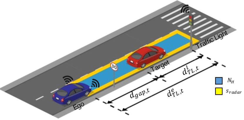
Figure 5: Schematic of the ego vehicle approaching a signalized intersection while following an unconnected target vehicle.

3.3 Methodology

A comprehensive vehicle trajectory dataset, Next Generation Simulation (NGSIM), was collected by U.S. Federal Highway Administration (FHWA) in 2005 and is widely used in transportation research, especially in traffic flow analysis and modelling, traffic-related estimation and prediction, and vehicular ad hoc network-related studies (Kovvali et al. (2007)). In this paper, a subset of the dataset is adopted to train the GRU-ED network.

The GRU-ED network is trained over approximately 18 hours of NGSIM driving data using TensorFlow and the Keras API package. To access the learning performance of the model and its ability to generalize over different drivers, the considered data-set is split into 70% for training the GRU-ED and 30% to validate and test the trained model. For better generalization over the different features, the feature set $\mathcal{F}$ is normalized between 0 and 1 using the sci-kit learn toolbox in Python. Custom functions are designed to split the data into a historical window and prediction window of time duration $T_{h}$ and $T_{p}$ respectively during the training phase. To evaluate the performance of the prediction model, Root Mean Square Error (RMSE) is computed between the predicted speed ($\hat{y}_{t}$) and the actual speed ($y_{t}$):

$$\text{RMSE}=\sqrt{\frac{1}{N}\sum_{i=1}^{N}(y_{t}-\hat{y}_{t})^{2}}$$ (4)

3.4 Evaluation

To analyze the effect of both $T_{h}$ and $T_{p}$ on the accuracy of prediction, a sensitivity study was performed where the GRU-ED network is trained and tested over several combinations of $[T_{h},T_{p}]$ pairs, as shown in Table 1.

For a given $T_{h}$, increasing the length of prediction window increases the RMSE. For instance, the pair $[T_{h},T_{p}]=[5s,5s]$ produces the lowest RMSE and as the length of prediction window increases for fixed $T_{h}$, the RMSE increases. However, for a given $T_{p}$, increasing the length of $T_{h}$ decreases the RMSE but the difference is not very large. This signifies that the network’s accuracy is more sensitive to the length of prediction window but less sensitive to the length of historical window.

Table 1: RMSE between predicted and actual velocity for different $T_{h}$ and $T_{p}$

[$T_{h},T_{p}$] [s,s]	[5,5]	[5,10]	[5,20]	[10,10]	[10,20]	[20,20]
RMSE [m/s]	0.77	1.85	3.45	1.83	3.44	3.36

Fig. 6 and Fig. 7 show the actual and predicted velocity comparison and the correlation plot respectively for $[T_{h},T_{p}]=[5s,5s]$. Clearly, the predictor is able to forecast most of the acceleration/deceleration/cruise events, but it diverges for small durations at points where the vehicle abruptly switches from an acceleration to a deceleration maneuver (or vice-versa). This is understandable, since the velocity predictor relies only on the current values of velocity and acceleration, hence large variations in magnitude and sign of the vehicle acceleration (for example occurring during a rapid transition from acceleration to braking) are impossible to predict with the available features. Nonetheless, the network converges to the actual velocity within the span of few seconds.

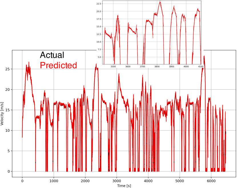
Figure 6: Comparison between the Predicted and Actual Velocity Trajectory.

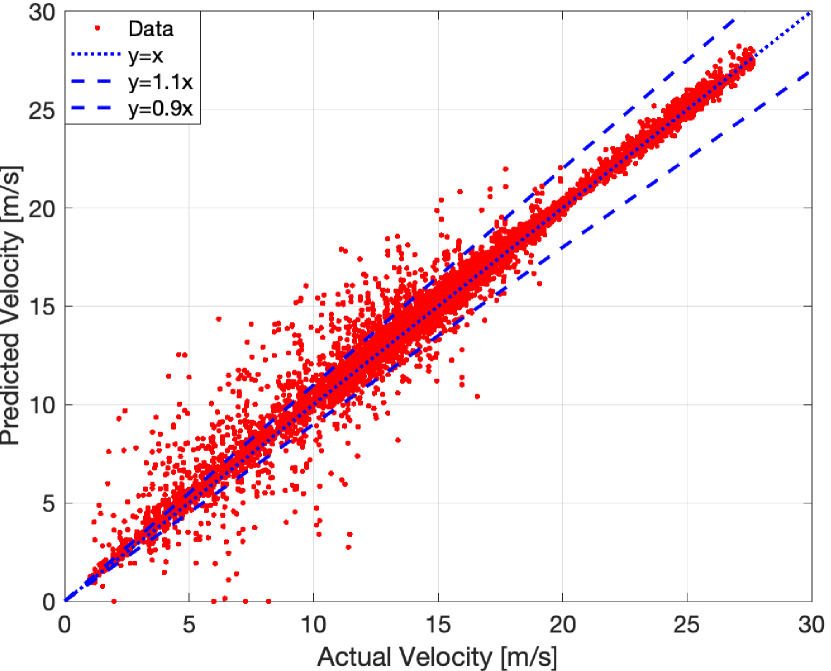
Figure 7: Correlation Plot for $T_{h}=5s$ and $T_{p}=5s$.

4 Integration with Eco-Driving Algorithm

The Eco-Driving algorithm implemented in this study is based on an Optimal Control Problem (OCP) formulated in spatial domain that minimizes fuel consumption over an entire route of N steps:

$$\min_{u_{s}}\sum_{s=1}^{s=N}{\left(\gamma\cdot\dot{m}_{\mathrm{f},s}+(1-\gamma)\right)\cdot\Delta t_{s}}$$ (5)

where $s$ is the discrete position, $u_{s}$ is the control input, $\gamma$ is a weighing factor between the fuel consumption and the travel time, and $\dot{m}_{\text{f},s}$ is the fuel flow rate. $\Delta t_{s}(:=\frac{\Delta d_{s}}{\bar{v}_{s}})$ is the travel time per step, $\Delta d_{s}$ is the distance step (i.e. $\Delta d_{s}=d_{s+1}-d_{s}$) calculated from the distance traveled ($d_{s}$) along the route at position $s$, and $\bar{v}_{s}=\frac{v_{s}+v_{s+1}}{2}$ is the average velocity. The state and action space are subject to a set of constraints, as described in Olin et al. (2019).

To incorporate time-based information such as SPaT and presence of other vehicles, time is added as an additional state variable in the OCP formulated in the spatial domain. In previous work, Zhu et al. (2021) formulated a 3 state OCP with time as one of the states to incorporate the SPaT information into the Eco-Driving controller, assuming a traffic-free environment. However, the effectiveness of this controller would reduce in presence of a target vehicle, particularly near signalized intersections. In this work, the target vehicle velocity predicted by the GRU-ED network is integrated with the Eco-Driving OCP and solved over a receding horizon of $N_{H}(N_{H}<<<N)$ steps to mitigate the aforementioned issue.

One way to incorporate target vehicle velocity information into the Eco-Driving controller would be to impose the predicted target vehicle velocity as a state constraint in the OCP, however this would likely result in an overly conservative design. For this reason, the target vehicle velocity trajectory ($\hat{v}^{l}_{s}$) predicted by the GRU-ED network is utilized within the Eco-driving controller to determine the relative distance $\hat{d}_{gap,s}$ between the lead and the ego vehicle, whose velocity ($v^{e}_{s}$) is computed as the solution of the receding horizon OCP.

To compute the relative distance $\hat{d}_{gap,s}$, let us consider that at a time $t_{s}$, the controller has the information about its current velocity $v^{e}_{s}$, current target vehicle velocity $v^{l}_{s}$ and the current distance gap $d_{gap,s}$ available from the on-board detection system. Further let us assume that the ego vehicle takes $\Delta t_{s}$ time to travel a distance step $\Delta d_{s}$ and reaches a velocity $v^{e}_{s+1}$ as shown in Fig. 8. The target vehicle velocity at time $t_{s+1}$ is obtained by interpolating the time-varying predicted velocity trajectory obtained from by GRU-ED network. The difference in the area between the ego and lead velocity-time curve would denote the change in relative distance $\Delta d_{gap,s}$ over the next distance step. At a given position $k$, the dynamic model for $d_{gap,k},\forall k=s,\cdots,s+N_{H}-1$ can be derived as:

$$\hat{d}_{gap,k+1} =\hat{d}_{gap,k}+(\bar{\hat{v}}_{k}^{l}-\bar{v}_{k}^{e})\Delta t_{k}$$ (6a)

$$=\hat{d}_{gap,k}+(\bar{\hat{v}}_{k}^{l}-\bar{v}_{k}^{e})\frac{\Delta d_{k}}{\bar{v}^{e}_{k}}$$ (6b)

$$=\hat{d}_{gap,k}+\left(\frac{\bar{\hat{v}}_{k}^{l}}{\bar{v}_{k}^{e}}-1\right){\Delta d_{k}}$$ (6c)

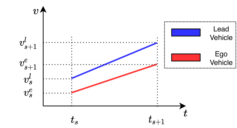
Figure 8: Ego and Target Vehicle Velocity over $\Delta d_{s}$.

Eqn. 6c represents the relative distance between the lead and ego vehicle at any point in a $N_{H}$ horizon, which varies as a function of the ratio of average lead and ego vehicle velocity evaluated over a distance step. If $\bar{\hat{v}}_{k}^{l}>\bar{v}_{k}^{e}$, the target vehicle is faster than ego vehicle and the $\hat{d}_{gap,{k+1}}>\hat{d}_{gap,{k}}$. On the other hand, if $\bar{\hat{v}}_{k}^{l}<\bar{v}_{k}^{e}$, the target vehicle is slower than ego vehicle and the $\hat{d}_{gap,{k+1}}<\hat{d}_{gap,{k}}$. This logic can be used by the Eco-Driving controller to modulate the ego vehicle velocity such that the $\hat{d}_{gap,{k}}>d_{safe,s}$ which is defined as the safe car-following distance (Brackstone and McDonald (1999)):

$$d_{safe,s}=d_{0}+v^{e}_{s+1}T_{\text{gap}}+\frac{v^{e}_{s+1}\Delta v_{s+1}}{2\sqrt{a_{\text{max}}b_{max}}}$$ (7)

where $d_{0}$ refers to the safe distance gap at stand still, $T_{gap}$ refers to the time gap, $\Delta v_{s+1}$ refers to the relative velocity between target and ego vehicle, $a_{\text{max}}$ and $b_{max}$ refers to the maximum acceleration and deceleration respectively. Assume that the discretized state dynamics for the Eco-Driving problem has the following form:

$$x_{s+1}=f_{s}(x_{s},u_{s}),\quad s=1,\cdots,N-1.$$ (8)

where $x_{s}=[v_{s},\xi_{s},t_{s}]^{\mathsf{T}}\in\mathcal{X}_{s}\subseteq\mathbb{R}^{p}$ and $u_{s}=[T_{\mathrm{eng},s},T_{\mathrm{bsg},s}]^{\mathsf{T}}\in\mathcal{U}_{s}\subseteq\mathbb{R}^{q}$ are the state and control actions respectively. In this work, the state variables are the vehicle velocity $(v_{s})$, battery SoC $(\xi_{s})$ and travel time $(t_{s})$. The control actions are the engine torque $(T_{\mathrm{eng},s})$ and BSG torque $(T_{\mathrm{bsg},s})$. The equations describing the state dynamics $f_{s}(x_{s},u_{s})$ have been derived in prior work (Gupta (2019)).

As mentioned above, the Eco-Driving optimization problem is formulated as a receding horizon optimal control problem where the full route of $N$ steps is solved over a reduced horizon $N_{H}(<<N)$. At a given position $s=1,\dots,N-N_{H}$, the optimization problem is formulated as:

$$\begin{gathered}\mathcal{J}^{*}(x_{s})=\min_{\left\{\mu_{k}\right\}_{k=s}^{s+N_{H}-1}}\sum_{k=s}^{s+N_{H}-1}c_{\mathrm{T}}(x_{s+N_{H}})+c(x_{k},\mu_{k}(x_{k})),\\ c(x_{k},\mu_{k}(x_{k}))=\left(\gamma\cdot\dot{m}_{\mathrm{f},k}(x_{k},\mu_{k}(x_{k}))+(1-\gamma)\right)\cdot\Delta t_{k}\end{gathered}$$ (9)

where $\mu_{k}:\mathcal{X}\rightarrow\mathcal{U}$ is the admissible control policy of the controller at the step $k$ in the prediction horizon; $c:\mathcal{X}\times\mathcal{U}\rightarrow\mathbb{R}$ is the stage cost function defined as the weighted average of the fuel consumption and travel time; $c_{\mathrm{T}}:\mathcal{X}\rightarrow\mathbb{R}$ is the terminal cost function. The state space and action space are subject to following constraints: $\forall s=1,\dots,N-N_{H}$, $\forall k=s,\dots,s+N_{H}$:

$$v_{k} \in[v_{k}^{\mathrm{min}},v_{k}^{\mathrm{max}}],$$ (10a)

$$\xi_{k} \in[\xi_{k}^{\mathrm{min}},\xi_{k}^{\mathrm{max}}],$$ (10b)

$$t_{k} \in\mathcal{T}_{\mathrm{G},k},$$ (10c)

$$a_{k} \in[a^{\mathrm{min}},a^{\mathrm{max}}],$$ (10d)

$$\hat{d}_{gap,k} \in[d_{\text{safe}},d_{\text{radar}}]$$ (10e)

$$T_{\mathrm{eng},k} \in[T_{\mathrm{eng}}^{\mathrm{min}}(v_{k}),T_{\mathrm{eng}}^{\mathrm{max}}(v_{k})],$$ (10f)

$$T_{\mathrm{bsg},k} \in[T_{\mathrm{bsg}}^{\mathrm{min}}(v_{k}),T_{\mathrm{bsg}}^{\mathrm{max}}(v_{k})],$$ (10g)

where $v^{\mathrm{min}}_{s},v^{\mathrm{max}}_{s}$ are the minimum and maximum route speed limits respectively, $\xi_{s}^{\mathrm{min}},\xi_{s}^{\mathrm{max}}$ are the static limits applied on battery SoC, $a^{\mathrm{min}},a^{\mathrm{max}}$ represent the limits imposed on the acceleration for comfort, $d_{\text{safe}}$ is obtained from Eqn. 7, $d_{radar}$ refers to the radar range (assumed to be 250m), $T_{\mathrm{eng}}^{\mathrm{min}}(v_{s}),T_{\mathrm{eng}}^{\mathrm{max}}(v_{s})$ are the minimum and maximum engine torque limits, and $T_{\mathrm{bsg}}^{\mathrm{min}}(v_{s}),T_{\mathrm{bsg}}^{\mathrm{max}}(v_{s})$ are the minimum and maximum BSG torque limits, respectively. To ensure SoC neutrality over the entire itinerary, a terminal constraint $\xi_{1}=\xi_{N}$ is applied to the battery. $\mathcal{T}_{\mathrm{G},s}$ represents the feasible set of travel time for passing-at-green at signalized intersections (Zhu et al. (2021)).

The receding horizon OCP is solved using Approximate Dynamic Programming (ADP), such that an approximate terminal cost used in the receding horizon OCP (named Short-term Optimization in Fig. 1) is obtained from the offline solution of a full-route optimization under partial information (termed Long-term Optimization).

5 Simulation and Evaluation of Results

To illustrate the proposed approach, a mixed-urban route in Columbus, OH (USA) was been selected for the simulation and analysis. As shown in Fig. 9, the route is 7km in length and comprises 5 traffic lights and 2 stop signs (start and end of the trip).

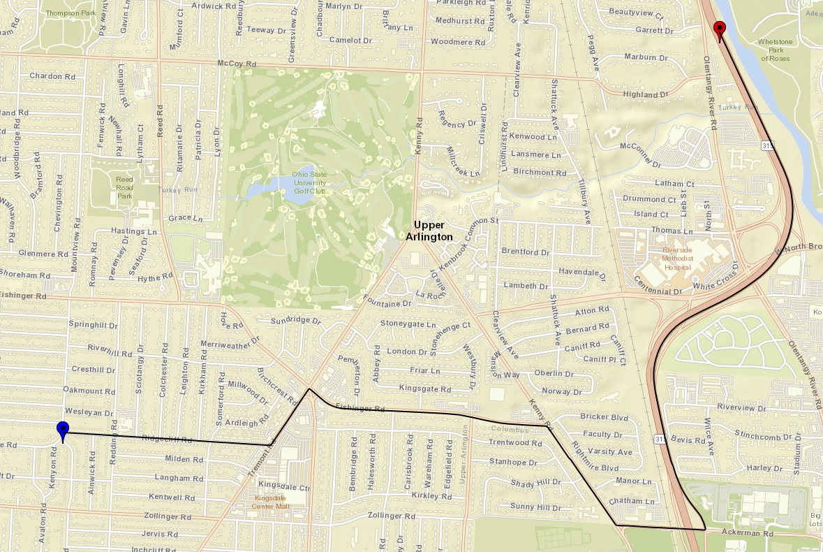
Figure 9: Selected route for simulation and validation on OpenStreetMaps (Route 19). Blue and red marker denote the start and destination respectively.

To simulate the presence of a target vehicle, a time-varying vehicle velocity profile is generated using Simulation of Urban MObility (SUMO) for a given departure time. The vehicle velocity profile generated in SUMO is used as the source for the velocity predictor integrated into the Eco-Driving controller. The velocity profile is segmented into historical data using a moving window of 10s, then fed to the trained GRU-ED network to predict the target vehicle velocity within the receding horizon OCP that determines the optimal speed and battery SoC profiles for the ego vehicle (Eqn. 9 and 10). Note that this framework is reasonable for this study, since the vehicle motion in the simulation is limited to a single lane and the SPaT sequences obtained from SUMO are post-processed to be consistent with the departure time of the target vehicle.

Fig. 10 shows the velocity trajectory and time-space plot of the lead and ego vehicle over the route shown in Fig. 9. The ego vehicle is able to pass all the traffic lights, except the second, at a green phase even in the presence of a target vehicle. Within the V2I communication range of the first, fourth and fifth traffic lights (located at approximately 1300, 3600, 3800m), the Eco-Driving controller is aware of the time remaining in the green phase. This information, combined with the GRU-ED network predicting the target vehicle to cruise (based on the historical data and distance to traffic light), is exploited by the Eco-Driving controller to either hold the ego vehicle speed or accelerate to pass the signalized intersections during the green phase. This is also evident from the Fig. 11, where the relative distance either remains the same or decreases.

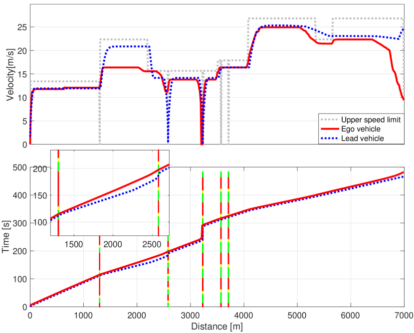
Figure 10: Speed trajectory and Time-Space plot showing the eco-driving manuever in presence of V2I communication and human-driven target vehicle over Route 19.

Moreover, while approaching the second traffic light, the Eco-Driving controller knows a priori that the time remaining in the red phase is small and the GRU-ED network predicts the target vehicle will decelerate (based on the initial deceleration of the target vehicle while approaching the intersection). Using this information, the controller lowers the ego vehicle’s speed to allow the signal to change to green, while at the same time avoiding a collision with the target vehicle. At the third traffic light, since the time remaining in the red phase is large, the Eco-Driving controller decides to stop, to avoid a collision with the target vehicle at the intersection. It should be noted that even during stand-still, the ego vehicle maintains a safe gap from the target vehicle.

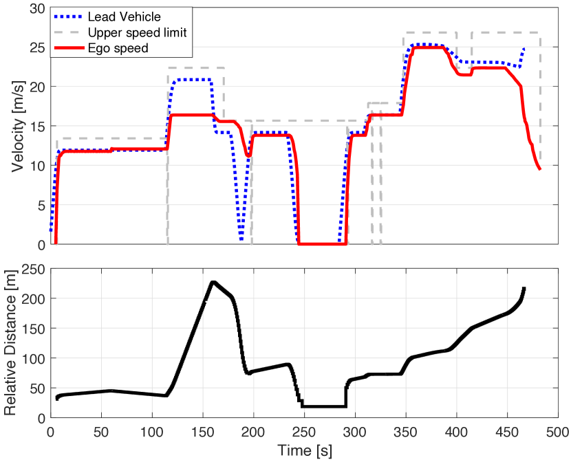
Figure 11: Speed trajectory and Relative Distance to the Target Vehicle over Route 19.

To evaluate the benefits of the integration of GRU-ED network with the Eco-Driving controller in terms of Fuel Consumption (FC) and Travel Time (TT), the simulation results were compared against a baseline case where the target vehicle velocity is assumed to be constant over the $N_{H}$ horizon and equal to the value detected at each time step. Table 2 compares the average FC and TT obtained with a constant velocity predictor and the GRU-ED network predictor while driving over the Route 19 for 5 different target vehicle velocity and signal phase departure times. Results show that the average TT and FC evaluated over the 5 scenarios for constant velocity case is approximately 7% and 3% respectively higher than the GRU-ED Network case. This indicates that the GRU-ED velocity forecast provides more opportunities for regen and minimizes unnecessary braking thereby improving the overall fuel economy in all aspect of the optimization. Further, the forecast of target vehicle velocity over the prediction horizon allows the ego vehicle to pass-at-green at most of the intersections when compared against the baseline case reducing overall travel time.

Table 2: Comparison of FC and TT with and w/o a lead velocity predictor over Route 19

Velocity Prediction Method	Fuel Consumption [g]	Tavel Time [s]
Constant Velocity	277	520
GRU-ED Network	268	486

6 Conclusions

In this work, an Eco-Driving strategy formulated for a connected and automated mild-HEV with an on-board detection system, V2I communication and longitudinal automation was augmented with a prediction-based target vehicle velocity estimator. A sequence-to-sequence velocity predictor, based upon a Gated Recurrent Encoder-Decoder (GRU-ED) network was trained to forecast the target vehicle velocity trajectory based upon historic data, and was then integrated with the Eco-Driving controller by designing a dynamic model of the relative distance between the target and the ego vehicle. Compared to previous studies where the target vehicle is assumed to be fully connected, the methodology proposed in this paper is applicable to the more general case of a target vehicle with partial or no automation, and without the ability to broadcast velocity and acceleration.

The Eco-Driving problem was cast as a receding horizon optimal control problem with three states, namely vehicle velocity, battery SoC and travel time. The problem was solved using Approximate Dynamic Programming and implemented in a Model Predictive Control (MPC) framework. It is worth mentioning that the formulation presented in this paper integrates all elements of the Eco-Driving problem (speed planning and powertrain set-points optimization) into a single controller. Simulation results indicate that the Eco-Driving controller is able to intelligently pass the signalized intersection in green phase, by forecasting the target vehicle velocity. Future work will address the development of a co-simulation platform where the optimization is performed in a parallel implementation developed with CUDA programming on a GPU to reduce the computational requirement from inclusion of additional states and allow to perform Eco-Driving in presence of multiple surrounding vehicles in a multi-lane scenario.

The authors acknowledge the support from the United States Department of Energy, Advanced Research Projects Agency – Energy (ARPA-E) NEXTCAR project (Award Number DE-AR0000794).

References

- Alam and McNabola (2014) Alam, M.S. and McNabola, A. (2014). A critical review and assessment of eco-driving policy & technology: Benefits & limitations. Transport Policy, 35, 42–49.
- Altché and de La Fortelle (2017) Altché, F. and de La Fortelle, A. (2017). An lstm network for highway trajectory prediction. In 2017 IEEE 20th International Conference on Intelligent Transportation Systems (ITSC), 353–359. IEEE.
- Brackstone and McDonald (1999) Brackstone, M. and McDonald, M. (1999). Car-following: a historical review. Transportation Research Part F: Traffic Psychology and Behaviour, 2(4), 181–196.
- Cho et al. (2014) Cho, K., Van Merriënboer, B., Gulcehre, C., Bahdanau, D., Bougares, F., Schwenk, H., and Bengio, Y. (2014). Learning phrase representations using rnn encoder-decoder for statistical machine translation. arXiv preprint arXiv:1406.1078.
- Chung et al. (2014) Chung, J., Gulcehre, C., Cho, K., and Bengio, Y. (2014). Empirical evaluation of gated recurrent neural networks on sequence modeling. arXiv preprint arXiv:1412.3555.
- Firoozi et al. (2018) Firoozi, R., Nazari, S., Guanetti, J., O’Gorman, R., and Borrelli, F. (2018). Safe adaptive cruise control with road grade preview and v2v communication. arXiv preprint arXiv:1810.09000.
- Gao et al. (2020) Gao, S., Huang, Y., Zhang, S., Han, J., Wang, G., Zhang, M., and Lin, Q. (2020). Short-term runoff prediction with gru and lstm networks without requiring time step optimization during sample generation. Journal of Hydrology, 589, 125188.
- Guanetti et al. (2018) Guanetti, J., Kim, Y., and Borrelli, F. (2018). Control of connected and automated vehicles: State of the art and future challenges. Annual reviews in control, 45, 18–40.
- Gupta (2019) Gupta, S. (2019). Look-Ahead Optimization of a Connected and Automated 48V Mild-Hybrid Electric Vehicle. Master thesis, The Ohio State University, USA.
- Gupta et al. (2019) Gupta, S., Deshpande, S.R., Tulpule, P., Canova, M., and Rizzoni, G. (2019). An enhanced driver model for evaluating fuel economy on real-world routes. IFAC-PapersOnLine, 52(5), 574–579.
- Gupta et al. (2020) Gupta, S., Deshpande, S.R., Tufano, D., Canova, M., Rizzoni, G., Aggoune, K., Olin, P., and Kirwan, J. (2020). Estimation of fuel economy on real-world routes for next-generation connected and automated hybrid powertrains. Technical report, SAE Technical Paper.
- Guzzella et al. (2007) Guzzella, L., Sciarretta, A., et al. (2007). Vehicle propulsion systems, volume 1. Springer.
- Hochreiter and Schmidhuber (1997) Hochreiter, S. and Schmidhuber, J. (1997). Long short-term memory. Neural computation, 9(8), 1735–1780.
- Hyeon et al. (2019) Hyeon, E., Kim, Y., Prakash, N., and Stefanopoulou, A.G. (2019). Influence of speed forecasting on the performance of ecological adaptive cruise control. In ASME 2019 Dynamic Systems and Control Conference. American Society of Mechanical Engineers Digital Collection.
- Hyeon et al. (2021) Hyeon, E., Shen, D., Karbowski, D., and Rousseau, A. (2021). Forecasting short to mid-length speed trajectories of preceding vehicle using v2x connectivity for eco-driving of electric vehicles. Technical report, SAE Technical Paper.
- Kamal et al. (2015) Kamal, M.A.S., Taguchi, S., and Yoshimura, T. (2015). Intersection vehicle cooperative eco-driving in the context of partially connected vehicle environment. In 2015 IEEE 18th International Conference on Intelligent Transportation Systems, 1261–1266. IEEE.
- Kovvali et al. (2007) Kovvali, V.G., Alexiadis, V., and Zhang PE, L. (2007). Video-based vehicle trajectory data collection. Technical report.
- Lefèvre et al. (2014) Lefèvre, S., Sun, C., Bajcsy, R., and Laugier, C. (2014). Comparison of parametric and non-parametric approaches for vehicle speed prediction. In 2014 American Control Conference, 3494–3499. IEEE.
- Olin et al. (2019) Olin, P., Aggoune, K., Tang, L., Confer, K., Kirwan, J., Deshpande, S.R., Gupta, S., Tulpule, P., Canova, M., and Rizzoni, G. (2019). Reducing fuel consumption by using information from connected and automated vehicle modules to optimize propulsion system control. Technical report, SAE Technical Paper.
- Pascanu et al. (2013) Pascanu, R., Mikolov, T., and Bengio, Y. (2013). On the difficulty of training recurrent neural networks. In International conference on machine learning, 1310–1318. PMLR.
- Rajakumar Deshpande et al. (2020) Rajakumar Deshpande, S., Gupta, S., Kibalama, D., Pivaro, N., and Canova, M. (2020). Benchmarking fuel economy of connected and automated vehicles in real world driving conditions via monte carlo simulation. In Dynamic Systems and Control Conference, volume 84270, V001T10A004. American Society of Mechanical Engineers.
- Sun et al. (2014) Sun, C., Hu, X., Moura, S.J., and Sun, F. (2014). Velocity predictors for predictive energy management in hybrid electric vehicles. IEEE Transactions on Control Systems Technology, 23(3), 1197–1204.
- Sutskever et al. (2014) Sutskever, I., Vinyals, O., and Le, Q.V. (2014). Sequence to sequence learning with neural networks. arXiv preprint arXiv:1409.3215.
- Toledo et al. (2007) Toledo, T., Koutsopoulos, H.N., and Ben-Akiva, M. (2007). Integrated driving behavior modeling. Transportation Research Part C: Emerging Technologies, 15(2), 96–112.
- Xu and Peng (2018) Xu, S. and Peng, H. (2018). Design and comparison of fuel-saving speed planning algorithms for automated vehicles. IEEE Access, 6, 9070–9080.
- Zhang et al. (2017) Zhang, J., Du, J., and Dai, L. (2017). A gru-based encoder-decoder approach with attention for online handwritten mathematical expression recognition. In 2017 14th IAPR International Conference on Document Analysis and Recognition (ICDAR), volume 1, 902–907. IEEE.
- Zhu et al. (2021) Zhu, Z., Gupta, S., Pivaro, N., Deshpande, S.R., and Canova, M. (2021). A gpu implementation of a look-ahead optimal controller for eco-driving based on dynamic programming. arXiv preprint arXiv:2104.01284.