An iterative Jacobi-like algorithm to compute a few sparse eigenvalue-eigenvector pairs

Abstract

In this paper, we describe a new algorithm to compute the extreme eigenvalue/eigenvector pairs of a symmetric matrix. The proposed algorithm can be viewed as an extension of the Jacobi transformation method for symmetric matrix diagonalization to the case where we want to compute just a few eigenvalues/eigenvectors. The method is also particularly well suited for the computation of sparse eigenspaces. We show the effectiveness of the method for sparse low-rank approximations and show applications to random symmetric matrices, graph Fourier transforms, and with the sparse principal component analysis in image classification experiments.

I Introduction

Low-rank eigenvalue decompositions (EVD) of matrices [1] are one of the most important algorithms in numerical linear algebra with many applications in applied mathematics, machine learning, and signal processing.

For full symmetric matrices, one of the most popular ways to build eigendecompositions is the QR algorithm [2, 3]. While this algorithm efficiently produces the complete eigenfactorization, it can be numerically expensive to run if the input matrix is very large or it has some special structure that is destroyed in the algorithm’s update steps. For sparse and/or large scale matrices, several methods have been proposed in the literature which compute just a few eigenvalues/eigenvectors pairs of interest (either a few of the extreme ones or a few near a given eigenvalue $\lambda$): iterative subspace methods [4, Chapter 7.3] with Rayleigh-Ritz acceleration [5], Lanczos methods [6] with restarts [7], Jacobi-Davidson methods [8, 9], Rayleigh quotient [10] and trace minimization [11] methods.

Introduced in 1848, the Jacobi method for the diagonalization of a symmetric matrix [12] is a conceptually simple yet effective method to find all the eigenvalues/eigenvectors of a symmetric matrix. It is based on iteratively canceling the largest absolute value off-diagonal element in the matrix until we are left only with the diagonal elements (up to some precision). Because it is relevant to our work here, we will give an overall description of this algorithm in Section II.

The topic is of great interest as there is still much research underway to perform faster [13], structured [14], and more robust decompositions [15] with modern applications [16]. In recent years, driven mostly by applications in machine learning and signal processing, researchers have started to explore algorithms and theory for the construction of sparse eigenspaces. In the era of big data, it is convenient to find eigenspaces that are easier to store (due to sparsity) and interpretable. To this end, the sparse principal component analysis (SPCA) method was introduced in [17] to build sparse eigenspaces. As SPCA involves a sparsity constraint, it is NP-hard to solve in general [18] and, therefore, there is continuous research to find better algorithms and tighter guarantees to find sparse principal components. There are several strategies proposed to solve the SPCA problem: the work in [19, 17] added an $\ell_{1}$ regularization to achieve sparsity, a direct formulation based on semidefinite programming [20], greedy methods for SPCA [21], iterative thresholding methods applied to the SVD [22, 23], and generalized power method framework [24].

In this paper, we propose an extension of the Jacobi method that computes only a few eigenvectors and is therefore well suited to build $p$-rank approximations. The method is also particularly well suited when searching for sparse eigenspaces.

The paper is organized as follows: Section II gives a brief outline of the Jacobi method for matrix diagonalization, Section III describes the main ideas of the paper and details the proposed algorithm, and finally, Section IV gives experimental evidence on the performance of the proposed method.

II The Jacobi method for the diagonalization of a symmetric matrix

The Jacobi eigenvalue algorithm is an iterative method that computes all the eigenvalues/eigenvectors of a real symmetric matrix. Starting from the given matrix $\mathbf{S}^{(0)}\leftarrow\mathbf{S}$ the algorithm proposes a series of updates like $\mathbf{S}^{(k)}\leftarrow\mathbf{J}_{ij}^{T}\mathbf{S}^{(k-1)}\mathbf{J}_{ij}$ where $\mathbf{J}_{ij}$ is called a Jacobi rotation matrix such that the entry $(i,j)$ of the matrix $\mathbf{S}^{(k)}$ is zeroed. At step $k$, we choose to zero the largest absolute value entry in the matrix, i.e., $(i,j)=\underset{q>t}{\arg\max}\ |S_{tq}^{(k)}|$, and therefore guaranteeing that the iterates converge to a diagonally dominant matrix, i.e., $\lim_{k\to\infty}\mathbf{S}^{(k)}=\mathbf{\Lambda}=\text{diag}(\mathbf{\lambda})$ (the diagonal of eigenvalues, but they are not in any particular order). The method converges linearly at first and quadratically after a certain number of updates [25]. Moreover, it can be implemented efficiently on a parallel computing architecture [26].

III The proposed method

In this section, we propose to modify the Jacobi method to compute only a few eigenvalues/eigenvectors. Similarly to the Jacobi method, we are concerned with two questions:

1. how to choose the indices $(i,j)$ on which to operate?

2. what operation to perform on these chosen indices?

We propose to discuss our contribution in three steps: 1) we write the eigenvalue problem as a least-squares problem whose solution is a $p$-rank eigenspace; 2) to solve this least-square problem, we introduce basic building blocks for which we have closed-form solutions; and 3) we show that the eigenspace can be written as a product of these basic building blocks and we give an efficient algorithm to construct it.

Result 1. Given a vector $\mathbf{\alpha}\in\mathbb{R}^{p}$ and a symmetric matrix $\mathbf{S}\in\mathbb{R}^{n\times n}$ with its eigenvalue decomposition $\mathbf{S}=\mathbf{U}\mathbf{\Lambda U}^{T}$ where $\lambda_{1}\geq\lambda_{2}\geq\dots\geq\lambda_{n}$, then the following optimization problem in the variable $\mathbf{\bar{U}}\in\mathbb{R}^{n\times n}$:

$$\underset{\mathbf{\bar{U}},\ \mathbf{\bar{U}}^{T}\mathbf{\bar{U}}=\mathbf{I}_{n}}{\text{minimize}}\ \|\begin{bmatrix}\text{diag}(\mathbf{\alpha})&\mathbf{0}_{p\times(n-p)}\\ \mathbf{0}_{(n-p)\times p}&\mathbf{0}_{(n-p)\times(n-p)}\end{bmatrix}-\mathbf{\bar{U}}^{T}\mathbf{S}\mathbf{\bar{U}}\|_{F}^{2},$$ (1)

has the following solutions and objective function values:

• $\mathbf{\alpha}\in\mathbb{R}_{+}^{p}$ is sorted increasing: $\mathbf{\bar{U}}$ contains the $p$ eigenvectors associated with the largest $p$ eigenvalues of $\mathbf{S}$ and the objective function value is $\sum_{q=1}^{p}(\alpha_{q}-\lambda_{q})^{2}+\sum_{q=p+1}^{n}\lambda_{q}^{2}$;

• $\mathbf{\alpha}\in\mathbb{R}_{-}^{p}$ is sorted decreasing: $\mathbf{\bar{U}}$ contains the $p$ eigenvectors associated with the smallest $p$ eigenvalues of $\mathbf{S}$ and the objective function value is $\sum_{q=1}^{n-p}\lambda_{q}^{2}+\sum_{q=1}^{p}(\alpha_{p-q+1}-\lambda_{n-p+q})^{2}$.

In both cases, the columns of $\mathbf{\bar{U}}$ are stored in the decreasing order of their associated eigenvalues.

Proof. We denote the left matrix by $\mathbf{A}$ and then we have the objective function $\|\mathbf{A}-\mathbf{\bar{U}}^{T}\mathbf{S}\mathbf{\bar{U}}\|_{F}^{2}=\|\mathbf{A}\|_{F}^{2}+\|\mathbf{S}\|_{F}^{2}-2\text{tr}(\mathbf{A}\mathbf{\bar{U}}^{T}\mathbf{S}\mathbf{\bar{U}})$. By the Courant-Fischer theorem [27, Corollary 4.3.39], we maximize the trace term by choosing $\mathbf{\bar{U}}$ to be $p$ eigenvectors of $\mathbf{S}$ such that $\text{tr}(\mathbf{A}\mathbf{\bar{U}}^{T}\mathbf{S}\mathbf{\bar{U}})=\sum_{i=1}^{p}\alpha_{i}\lambda_{\sigma(i)}$ is largest for some ordering $\sigma$. To maximize the trace, the ordering is such that either the largest eigenvalues are picked (when $\alpha_{i}$ is positive) or the smallest eigenvalues (when $\alpha_{i}$ is negative). Eigenvalues/eigenvectors can be chosen in order to minimize the objective function as described in the result.$\hfill\blacksquare$

Result 2. Assume that $\mathbf{\bar{U}}$ in (1) has the following structure:

$$\mathbf{\bar{U}}=\mathbf{G}_{ij}=\begin{bmatrix}\mathbf{I}_{i-1}& &&\\ &*&&* \\ &&\mathbf{I}_{j-i-1}&\\ &*& &* \\ &&&&\mathbf{I}_{n-j}\\ \end{bmatrix},$$ (2)

with $\mathbf{\tilde{G}}\in\left\{\begin{bmatrix}c&-s\\ s&c\end{bmatrix},\begin{bmatrix}c&s\\ s&-c\end{bmatrix} \right\}$, such that $c^{2}+s^{2}=1$, where the non-zero part (denoted by $*$ and $\mathbf{\tilde{G}}$) is only on rows and columns $i$ and $j$. Then, the objective function of (1) is minimized when the non-trial part of $\mathbf{G}_{ij}$ is set to

$$\!\mathbf{\tilde{G}}\!=\!\mathbf{V}^{T}\!\text{ from a }2\times 2\text{ EVD of } \mathbf{S}_{\{i,j\}}\!\!=\!\!\begin{bmatrix}S_{ii}&S_{ij}\\ S_{ji}&S_{jj}\end{bmatrix}\!\!=\!\!\mathbf{VDV}^{T},$$ (3)

and, denoting the the left-hand side with $\mathbf{A}$ (a diagonal matrix such that $A_{ii}=\alpha_{i}$ for $i\leq p$ and $A_{ii}=0$ otherwise), we have that the minimum of (1) is:

$$\min\|\mathbf{A}-\mathbf{G}_{ij}^{T}\mathbf{S}\mathbf{G}_{ij}\|_{F}^{2}\!=\!\|\mathbf{\alpha}\|_{2}^{2}+\|\mathbf{\lambda}\|_{2}^{2}-2\sum_{q=1}^{p}\!\!\alpha_{q}S_{qq}-\mathcal{C}_{ij},$$ (4)

$$\!\!\text{ with }\mathcal{C}_{ij}\!=\!(A_{jj}-A_{ii})(S_{ii}-S_{jj}\!+\sqrt{(S_{ii}\!-S_{jj})^{2}\!+4S_{ij}^{2}}),$$ (5)

for $n\geq i>j$ and $\mathcal{C}_{ij}=0$ for all $i>p$.

Proof. We follow [28] and the proof structure given for Theorem 1 of [29] and develop the objective function in (4) to $\|\mathbf{A}-\mathbf{G}_{ij}\mathbf{S}\mathbf{G}_{ij}^{T}\|_{F}^{2}=\|\mathbf{\alpha}\|_{2}^{2}+\|\mathbf{\lambda}\|_{2}^{2}-2\text{tr}(\mathbf{Z})-2\mathcal{C}_{ij}$, where we have defined $\mathbf{Z}=\mathbf{AS}$ (we have $\text{tr}(\mathbf{AS})=\sum_{q=1}^{p}\alpha_{q}S_{qq}$) and the cost $\mathcal{C}_{ij}\!=\!\text{tr}(\mathbf{\tilde{G}}\mathbf{S}_{\{i,j\}}\!\mathbf{\tilde{G}}^{T}\text{diag}(\begin{bmatrix}A_{ii}&A_{jj}\end{bmatrix})-Z_{ii}\!-\!Z_{jj}$. The trace term develops to $\text{tr}(\mathbf{V}^{T}\mathbf{S}_{\{i,j\}}\mathbf{V}\text{diag}(\begin{bmatrix}A_{ii}&A_{jj}\end{bmatrix}))=\text{tr}(\!\mathbf{V}^{T}\mathbf{V}\mathbf{D}\!\mathbf{V}^{T}\mathbf{V}\text{diag}(\begin{bmatrix}A_{ii}&A_{jj}\end{bmatrix}))= \text{tr}(\mathbf{D}\text{diag}(\begin{bmatrix}A_{ii}&\!\!A_{jj}\end{bmatrix}))=\text{tr}(\text{diag}(\mathbf{d})\text{diag}(\begin{bmatrix}A_{ii}&\!\!A_{jj}\end{bmatrix}))\!\!=\!\!\! \begin{bmatrix}A_{ii}&A_{jj}\end{bmatrix}^{T}\mathbf{d}.$ Therefore, the cost is $\mathcal{C}_{ij}\!\!=\!\!\begin{bmatrix}A_{ii}&A_{jj}\end{bmatrix}^{T}\!\!\mathbf{d}\!-\!Z_{ii}\!-\!Z_{jj}\!=\begin{bmatrix}A_{ii}&A_{jj}\end{bmatrix}^{T}\!\begin{bmatrix}-\gamma_{ij} \\ \gamma_{ij}\end{bmatrix}=\frac{1}{2}(A_{jj}-A_{ii})$$\left(S_{ii} -S_{jj}+\sqrt{ S_{ii} -S_{jj}+4S_{ij}^{2}}\right)$, and we noticed that $Z_{ii}=A_{ii}S_{ii}$ and $Z_{jj}=A_{jj}S_{jj}$. The eigenvalues of $\mathbf{S}_{\{i,j\}}$ in $\mathbf{d}$ are computed by explicit formulas. Therefore, the minimizer of (4) is given in (3).$\hfill\blacksquare$

Remark 1 (Modification of the scores $\mathcal{C}_{ij}$). As discussed in Result 1 for (1), we would exactly minimize the objective function if $\mathbf{\alpha}$ would contain $p$ eigenvalues of $\mathbf{S}$ but we assume that these are not available apriori. Therefore we are in a situation where after applying a transformation on indices $(i,j)$ the new score on those indices is not zero (it is actually $2(S_{ii}-S_{jj})$, assuming $S_{ii}\geq S_{jj}$). To guarantee that the appropriate scores are zero, instead of (5), we use:

$$\mathcal{C}_{ij}=(A_{jj}-A_{ii})(\sqrt{(S_{ii}-S_{jj})^{2}+4S_{ij}^{2}}-(S_{ii}-S_{jj})).$$ (6)

This new score is zero when $S_{ij}$ is zero and the diagonal elements $S_{ii}$ and $S_{jj}$ are in decreasing order. These are the only cases when improvement in the objective function cannot be achieved. Otherwise, the scores are strictly positive. By construction we have that the $(i,j)^{\text{th}}$ element of $\mathbf{G}_{ij}^{T}\mathbf{S}\mathbf{G}_{ij}$ is set to zero (and the new diagonal elements are $\mathbf{D}$ from (3)).$\hfill\blacksquare$

Result 3. Assume now that $\mathbf{\bar{U}}$ in (1) is written as:

$$\mathbf{\bar{U}}=\prod_{q=1}^{k}\mathbf{G}_{i_{q}j_{q}}=\mathbf{G}_{i_{1}j_{1}}\mathbf{G}_{i_{2}j_{2}}\dots\mathbf{G}_{i_{k}j_{k}},$$ (7)

then we can solve (4) several times: at step $q$ we minimize $\|\mathbf{A}-\mathbf{G}_{i_{q}j_{q}}^{T}\mathbf{S}^{(q-1)}\mathbf{G}_{i_{q}j_{q}}\|_{F}^{2}$ where $\mathbf{S}^{(q-1)} = \mathbf{G}_{i_{q-1}j_{q-1}}^{T}\dots\mathbf{G}_{i_{1}j_{1}}^{T}\mathbf{S} \mathbf{G}_{i_{1}j_{1}} \dots\mathbf{G}_{i_{q-1}j_{q-1}}$. Similarly to the Jacobi method, our updates are $\mathbf{S}^{(q)}\leftarrow\mathbf{G}_{i_{q}j_{q}}^{T}\mathbf{S}^{(q-1)}\mathbf{G}_{i_{q}j_{q}}$.$\hfill\blacksquare$

Based on these results, we give the full description of the proposed method in Algorithm 1. We first compute all the scores $\mathcal{C}_{ij}$ which takes order $O(pn)$ operations and then proceed with the iterative phase where we apply a single (3) to the symmetric input matrix $\mathbf{S}$ – this takes $O(n)$ operations. Finally, only scores that have indices $(i,j)$ previously used are updated (all other scores remain the same) – this again takes $O(n)$. Therefore the computational complexity of Algorithm 1 is $O(n(p+q))$. Depending on the application, we usually have that $p\sim O(1)$ and we suggest taking $k\sim O(n\log_{2}n)$ to balance the accuracy of the eigenspace with its sparsity, see the Experimental Results section. Some remarks are in order.

Algorithm 1
Input: Symmetric matrix $\mathbf{S}\in\mathbb{R}^{n\times n}$, dimension of eigenspace $p\in\mathbb{N}^{*}$, target $\alpha\in\mathbb{R}^{p}$, and number of basic transformations/iterations $k\geq 1$.
Output: Approximate eigenspace $\mathbf{\bar{U}}\in\mathbb{R}^{n\times p}$ as (7).

1. Initialize: $\mathbf{\bar{U}}\leftarrow\mathbf{I}_{n}$, $\mathbf{S}^{(0)}\leftarrow\mathbf{S}$, $\mathcal{C}_{ij}$ with (6) for $j>i\geq p$.

2. Iterative process, for $q=1,\dots,k:$

• Find $(i_{q}^{\star},j_{q}^{\star})=\underset{i,j}{\arg\max}\ \mathcal{C}_{ij}$.

• Build $\mathbf{G}_{i_{q}^{\star}j_{q}^{\star}}$ according to (2) and (3) using $\mathbf{S}^{(q-1)}$.

• Update $\mathbf{S}^{(q)}\leftarrow\mathbf{G}_{i_{q}^{\star}j_{q}^{\star}}^{T}\mathbf{S}^{(q-1)}\mathbf{G}_{i_{q}^{\star}j_{q}^{\star}}$ and $\mathbf{\bar{U}}\leftarrow\mathbf{\bar{U}}\mathbf{G}_{i_{q}^{\star}j_{q}^{\star}}$.

• With (6), update $\mathcal{C}_{i_{q}^{\star}j}$ for $j>i_{q}^{\star}$ and $\mathcal{C}_{ij_{q}^{\star}}$ for $i\leq p$.

Remark 2 (The connection to the Jacobi method). Similarly to the Jacobi method, Algorithm 1 also has two steps: find indices $(i,j)$ and apply a transformation such that we are closer to the stated objective (diagonalize the matrix). But we differ from the Jacobi method in both steps: the selection of the indices is made with (6) instead of the maximum absolute value off-diagonal element and the transformation is not a Jacobi rotations but it is (3) (a general $2\times 2$ orthonormal transformation: rotation or reflection). Regarding these scores, we have that $\mathcal{C}_{ij}=|S_{ij}|$ like in the Jacobi method when $S_{ii}=S_{jj}$. Despite these differences, our method can also benefit from the parallelization techniques developed for the Jacobi method [26, 30].$\hfill\blacksquare$

Remark 3 (On the convergence of Algorithm 1). Because at each step of the proposed algorithm we make choices to maximally reduce the objective function in (4) we are guaranteed to converge to the solution. As long as some $C_{ij}>0$ progress is possible and these scores (6) are non-zero as long as there is at least one off-diagonal element $|S_{ij}|>0$. As the Jacobi method cancels at each step the largest off-diagonal element, its analysis was done differently, using the off-diagonal “norm” $\sqrt{\sum_{i=1}^{n}\sum_{j>i}^{n}|S_{ij}|^{2}}$ (we note that in our scenario $i$ goes only until $p$ and not $n$). In this quantity, first, linear convergence of the Jacobi method was proved [25] and then several researchers have shown quadratic convergence after a certain number of Jacobi steps [31, 32, 33, 34, 35]. For our method, if we want to recover the dense eigenvectors (we choose $k\sim O(n^{2})$), the quadratic results still hold and depend on the gap $|\lambda_{p}-\lambda_{p+1}|$ for the choice of $\mathbf{\alpha}$: with $\mathbf{\alpha}=\mathbf{1}_{p\times 1}$ or $\mathbf{\alpha}=-\mathbf{1}_{p\times 1}$ (see also next Remark 4). Otherwise, when we recover sparse eigenspaces with small $k$ (as with $k\sim O(n)$ or $k\sim O(n\log_{2}n)$) these convergence results do not hold.$\hfill\blacksquare$

Remark 4 (On the choice of $\mathbf{\alpha}$). As it is clear from Result 1 that it would be ideal to have the true eigenvalues of $\mathbf{S}$ for which we want to recover the eigenvectors. Unfortunately, these are not available in general. Therefore we propose two ways of choosing $\mathbf{\alpha}$: i) either $\alpha_{i}\in\{\pm 1\}$ (as per Result 1, to recover highest and lowest eigenvalues, respectively) or ii) $\mathbf{\alpha}$ is a decreasing/increasing series. In the first case, if the entries of $\mathbf{\alpha}$ are equal then $\mathcal{C}_{ij}=0$ for all $i,j\leq p$ and therefore we have that $\lim_{k\to\infty}\mathbf{S}^{(k)}=\begin{bmatrix}\mathbf{S}_{1}&\mathbf{0}_{p\times(n-p)}\\ \mathbf{0}_{(n-p)\times p}&\mathbf{S}_{2}\end{bmatrix}$ where the two blocks $\mathbf{S}_{1}\in\mathbb{R}^{p\times p}$ and $\mathbf{S}_{2}\in\mathbb{R}^{(n-p)\times(n-p)}$ are symmetric and they split the $n$ eigenvalues of $\mathbf{S}$. This means that we do not compute the eigenvectors, but a linear combination of the eigenvectors (in some applications, like principal component analysis [36, 37], this is sufficient). In the second case, we have in general that $\mathcal{C}_{ij}\neq 0$ for $j>i\geq 1$ and therefore we reach $\lim_{k\to\infty}\mathbf{S}^{(k)}=\begin{bmatrix}\mathbf{D}_{1}&\mathbf{0}_{p\times(n-p)}\\ \mathbf{0}_{(n-p)\times p}&\mathbf{S}_{3}\end{bmatrix}$ where now $\mathbf{D}_{1}\in\mathbb{R}^{p\times p}$ is the diagonal with $p$ eigenvalues and we therefore recover their actual $p$ eigenvectors. We note that if $\alpha_{1}=1$, $\alpha_{2}=-1$ and the rest are zero then Algorithm 1 approximates both the extreme eigenvalue/vector pairs simultaneously.$\hfill\blacksquare$

Remark 5 (A block version of Algorithm 1). In Algorithm 1 we have chosen indices two at a time. We can extend the method to deal with blocks of size $b\times b$ just as in block Jacobi methods [38, 35, 39]. In this case, we do assume we have a procedure to perform the EVD of a $b\times b$ matrix (the simple formulas of the $2\times 2$ case are no longer available). A natural way is to choose blocks of size $b=2p$ such that we pick $p$ pairs like $(i,\underset{j}{\arg\max}\ \mathcal{C}_{ij})$ for all $i\leq p$ (restricting such that no duplicate indices appear). In this case, we do compute the explicit eigenvectors and therefore the choice of $\mathbf{\alpha}$ is not relevant to the final result (we are in the second case of Remark 4).$\hfill\blacksquare$

Remark 6 (Algorithm 1 for large sparse matrices). When the given $\mathbf{S}$ is a large sparse matrix we are concerned with the fill-in that happens during Algorithm 1. We note that, at each step, the fill-in is at most $O(n)$. Regarding the scores, we have that most $S_{ij}=0$ and therefore the critical quantity in (6) which is $|S_{ii}-S_{jj}|-(S_{ii}-S_{jj})$ takes either the value 0 when the diagonal entries are ordered decreasing, i.e., $S_{ii}>S_{jj}$), or $2(S_{jj}-S_{ii})$ otherwise (in this case, the $\mathbf{G}_{ij}$ in (3) is a reflector that flips rows/columns $i$ and $j$ in $\mathbf{S}$, ensuring a diagonal with decreasing elements). Therefore, by ordering the diagonal entries of $\mathbf{S}$ we can have exactly as many non-zero scores $\mathcal{C}_{ij}$ as non-zero off-diagonal entries $S_{ij}$.$\hfill\blacksquare$

Remark 7 (Sparse eigenspaces and sweeping the indices). Maximizing the scores leads to the best possible update at each step of the algorithm and can be exploited to build sparse eigenspaces (we stop after just a few transformations $k\ll n^{2}$). Still, this step can be expensive as the maximum score needs to be found at each iteration. Furthermore, if we look to approximate the eigenspace giving up sparsity then sweeping all the indices in order is an appropriate solution (analogously to cyclic Jacobi algorithms [40, 41]). $\hfill\blacksquare$

Remark 8 (Algorithm 1 for Hermitian matrices). As with the Jacobi method for complex-valued matrices [25], the proposed algorithm is immediately extensible to the Hermitian case. In (6), for Hermitian $\mathbf{S}\in\mathbb{C}^{n\times n}$ we have that $\mathcal{C}_{ij}=(A_{jj}-A_{ii})(\sqrt{(S_{ii}-S_{jj})^{2}+4|S_{ij}|^{2}}-(S_{ii}-S_{jj}))$ and then the decomposition in (3) is over the complex field.$\hfill\blacksquare$

IV Experimental results

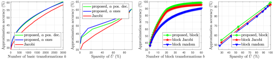
Figure 1: Average approximation accuracy (8) over 10 realizations for random matrices of size $n=1024$ when recovering $p=20$ eigenvectors associated with the highest eigenvalues. For the proposed method we show simulations for $\mathbf{\alpha}=\mathbf{1}_{p\times 1}$ and $\mathbf{\alpha}=\log_{2}(p+1,\dots,2)$ (a positive decreasing sequence). From left to right: evolution of (8) with the number of transformations $k$ in the approximation $\mathbf{\bar{U}}$; the sparsity of the eigenspace (number of non-zero elements in $\mathbf{\bar{U}}$ from the total number $np$); evolution of (8) for the block variant of the proposed method with block size $b=2p$; sparsity of the eigenspace created via the block proposed method (see Remark 5).

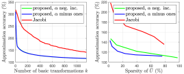
Figure 2: Average approximation accuracy (8) over 10 realizations for random community graphs of size $n=256$ created via the GSP Toolbox when recovering $p=32$ eigenvectors associated with the lowest eigenvalues of the graph Laplacians $\mathbf{L}$. We show accuracy as a function of number of transformations $k$ (left) and the sparsity of the eigenspace (right). Here, lower is better and $100\%$ means perfect recovery of all $p$ smallest eigenvalues.

In this section, we use the proposed method to construct low-rank approximations of 1) random matrices; 2) Laplacian matrices of random graphs; 3) covariance matrices in the context of principal component analysis (PCA) as a dimensionality reduction techniques before classification. To measure the quality of the eigenspace approximation $\mathbf{\bar{U}}$ we construct for a given $\mathbf{S}$, we use the approximation accuracy:

$$\epsilon(\mathbf{S},\mathbf{\bar{U}})=\frac{\text{tr}(\mathbf{\bar{U}}^{T}\mathbf{S\bar{U}})}{\sum_{i=1}^{p}\lambda_{p}}\ (\%).$$ (8)

The eigenvalues $\lambda_{i}$ can be either the lowest or highest of $\mathbf{S}$ and we assume $\sum_{i=1}^{p}\lambda_{i}\neq 0$, i..e, we are not trying to recover the null space of $\mathbf{S}$ of size $p$. Good approximations are obtained whenever $\epsilon\approx 1$ (or $100\%$). We will always compare with the classic Jacobi method (search for the maximum absolute off-diagonal element but using (3)). Full source code is online.

IV-1 Low-rank approximations of random symmetric matrices

We generate random matrices $\mathbf{X}\in\mathbb{R}^{n\times n}$ with entries drawn i.i.d. from the standard Gaussian distribution, then initialize $\mathbf{S}\leftarrow\mathbf{X}\mathbf{X}^{T}$ and we build rank $p=20$ approximations of $\mathbf{S}$. In Figure 1 we show the results obtained in the decomposition of these random matrices for $n=1024$. We compare against the Jacobi method and also show the block variant of the proposed method (see Remark 5). We always perform better than the Jacobi method in these experiments, showing that selecting indices via (6) brings benefits.

IV-2 Graph Fourier transforms: eigenvectors of graph Laplacians

In many graph signal processing applications [42, 43, 44], we are interested in estimating the eigenvectors associated with the lowest eigenvalues of an undirected graph Laplacian $\mathbf{L}$. These eigenvectors are define the graph Fourier transform [45] and are useful as they provide “low-frequency” information about graph signals. We generate random community graphs of $n=256$ nodes with the Graph Signal Processing Toolbox for which we decompose the sparse positive semidefinite Laplacians as $\mathbf{L}=\mathbf{U\Lambda U}^{T}$ and recover the eigenvectors from $\mathbf{U}$ associated with the lowest eigenvalues from $\mathbf{\Lambda}$. To compute the lowest eigenvalues we take Algorithm 1 with $\mathbf{\alpha}=-\mathbf{1}_{p\times 1}$ and $\mathbf{\alpha}=-\log_{2}(p+1,\dots,2)$ (a negative increasing sequence), same as taking $-\mathbf{L}$ instead of $\mathbf{L}$.

IV-3 Dimensionality reduction via sparse PCA

In the context of machine learning applications, given a dataset, it is important to compute the eigenvectors associated with the highest eigenvalues of the covariance matrix. We consider a classification example with the USPS dataset with 10 classes for which $n=256$ and the number of data points is $N=9298$. From the data matrix $\mathbf{X}\in\mathbb{R}^{n\times N}$ we explicitly compute the covariance $\mathbf{C}=\mathbf{X}\mathbf{X}^{T}$ and apply Algorithm 1 on $\mathbf{C}$ to get the $p$ principal components. We use the $K$-nearest neighbors ($K$-NN) classification algorithm with $K=15$, but before we perform dimensionality reduction with $p=15$. Results are shown in Figure 3. We compare against the full PCA, the sparse Johnson-Lindenstrauss (S-JL) transform [46] for $p=30$ components (for $p=20$ as with PCA the performance is poor because S-JL is not data dependent) with sparsity $s=3$ per column (overall sparsity $30\%$).

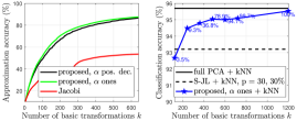
Figure 3: Average approximation accuracy (8) and average classification accuracy, on the left and right respectively, over 10 random realizations obtained by the proposed algorithm and with $K$-NN for the USPS dataset split into $N_{\text{train}}=8000$ and $N_{\text{test}}=1298$ after dimensionality reduction with $p=20$ was performed. Percentages on the plot shown in blue represent the sparsity of the eigenspace.

V Conclusions

In this paper, we have described an extension of the Jacobi method for the diagonalization of matrices for the computation just of a few eigenvalue/eigenvector pairs of a symmetric (or Hermitian) matrix. We show experimental results where we recover sparse eigenspaces associated with both of the highest and lowest eigenvalues and we highlight a trade-off between sparsity and eigenspace recovery accuracy.

References

- [1] G. H. Golub and H. A. Van der Vorst, “Eigenvalue computation in the 20th century,” Journal of Computational and Applied Mathematics, vol. 123, no. 1-2, pp. 35–65, 2000.
- [2] J. G. F. Francis, “The QR transformation - Part 1 and 2,” The Computer Journal, vol. 4, pp. 265–271 and 332–345, 1961-1962.
- [3] B. N. Parlett, “The QR algorithm,” Computing in Science Engineering, vol. 2, no. 1, pp. 38–42, 2000.
- [4] G. H. Golub and C. F. van Loan, Matrix Computations, Johns Hopkins University Press, 2012.
- [5] H. Rutishauser, “Simultaneous iteration method for symmetric matrices,” Numer. Math., vol. 16, no. 3, pp. 205–223, Dec. 1970.
- [6] H. D. Simon, “Analysis of the symmetric Lanczos algorithm with reorthogonalization methods,” Linear Algebra and its Applications, vol. 61, pp. 101–131, 1984.
- [7] K. Wu and S. D. Horst, “Thick-restart Lanczos method for symmetric eigenvalue problems,” in Solving Irregularly Structured Problems in Parallel, Alfonso Ferreira, José Rolim, Horst Simon, and Shang-Hua Teng, Eds., Berlin, Heidelberg, 1998, pp. 43–55, Springer Berlin Heidelberg.
- [8] G. L. G. Sleijpen and H. A. Van der Vorst, “A Jacobi-Davidson iteration method for linear eigenvalue problems,” SIAM Review, vol. 42, no. 2, pp. 267–293, 2000.
- [9] M. Ravibabu and A. Singh, “The least squares and line search in extracting eigenpairs in Jacobi–Davidson method,” Bit Numer. Math., vol. 60, no. 4, pp. 1033–1055, 2020.
- [10] D. E. Longsine and S. F. McCormick, “Simultaneous rayleigh-quotient minimization methods for Ax=Bx,” Linear Algebra and its Applications, vol. 34, pp. 195–234, 1980.
- [11] A. Sameh and Z. Tong, “The trace minimization method for the symmetric generalized eigenvalue problem,” Journal of Computational and Applied Mathematics, vol. 123, no. 1, pp. 155–175, 2000, Numerical Analysis 2000. Vol. III: Linear Algebra.
- [12] C. Jacobi, “Uber ein leichtes Verfahren die in der Theorie der Sacularstorungen vorkommenden Gleichungen numerisch aufzulosen,” Journal fur die reine und angewandte Mathematik, vol. 30, pp. 51–94, 1846.
- [13] M. F. Kaloorazi and J. Chen, “Efficient low-rank approximation of matrices based on randomized pivoted decomposition,” IEEE Transactions on Signal Processing, vol. 68, pp. 3575–3589, 2020.
- [14] M. Jacob, M. P. Mani, and J. C. Ye, “Structured low-rank algorithms: Theory, magnetic resonance applications, and links to machine learning,” IEEE Signal Processing Magazine, vol. 37, no. 1, pp. 54–68, 2020.
- [15] M. Huang, S. Ma, and L. Lai, “Robust low-rank matrix completion via an alternating manifold proximal gradient continuation method,” IEEE Transactions on Signal Processing, vol. 69, pp. 2639–2652, 2021.
- [16] R. Liu and N.-M. Cheung, “Joint estimation of low-rank components and connectivity graph in high-dimensional graph signals: Application to brain imaging,” Signal Processing, vol. 182, pp. 107931, 2021.
- [17] H. Zou, T. Hastie, and R. Tibshirani, “Sparse principal component analysis,” Journal of Computational and Graphical Statistics, vol. 15, no. 2, pp. 265–286, 2006.
- [18] A. M. Tillmann and M. E. Pfetsch, “The computational complexity of the restricted isometry property, the nullspace property, and related concepts in compressed sensing,” IEEE Transactions on Information Theory, vol. 60, no. 2, pp. 1248–1259, 2014.
- [19] I. T. Jolliffe, N. T. Trendafilov, and M. Uddin, “A modified principal component technique based on the LASSO,” Journal of Computational and Graphical Statistics, vol. 12, no. 3, pp. 531–547, 2003.
- [20] A. d’Aspremont, L. El Ghaoui, M. I. Jordan, and G. R. G. Lanckriet, “A direct formulation for sparse PCA using semidefinite programming,” SIAM Review, vol. 49, no. 3, pp. 434–448, 2007.
- [21] B. Moghaddam, Y. Weiss, and S. Avidan, “Spectral bounds for sparse PCA: Exact and greedy algorithms,” in Advances in Neural Information Processing Systems, Y. Weiss, B. Schölkopf, and J. Platt, Eds. 2006, vol. 18, MIT Press.
- [22] H. Shen and J. Z. Huang, “Sparse principal component analysis via regularized low rank matrix approximation,” Journal of Multivariate Analysis, vol. 99, no. 6, pp. 1015–1034, 2008.
- [23] D. M. Witten, R. Tibshirani, and T. Hastie, “A penalized matrix decomposition, with applications to sparse principal components and canonical correlation analysis,” Biostatistics, vol. 10, no. 3, pp. 515–534, 2009.
- [24] M. Journée, Y. Nesterov, P. Richtárik, and R. Sepulchre, “Generalized power method for sparse principal component analysis,” J. Mach. Learn. Res., vol. 11, pp. 517–553, 2010.
- [25] P. Henrici, “On the speed of convergence of cyclic and quasicyclic Jacobi methods for computing eigenvalues of Hermitian matrices,” Journal of the Society for Industrial and Applied Mathematics, vol. 6, no. 2, pp. 144–162, 1958.
- [26] G. Shroff, “A parallel algorithm for the eigenvalues and eigenvectors of a general complex matrix,” Numerische Mathematik, vol. 58, pp. 779–805, 1990.
- [27] R. A. Horn and C. R. Johnson, Matrix analysis, Cambridge University Press, 2013.
- [28] C. Rusu and L. Rosasco, “Fast approximation of orthogonal matrices and application to PCA,” arXiv:1907.08697, 2019.
- [29] C. Rusu and L. Rosasco, “Constructing fast approximate eigenspaces with application to the fast graph Fourier transforms,” arXiv:2002.09723, 2020.
- [30] Z. Shi, Q. He, and Y. Liu, “Accelerating parallel Jacobi method for matrix eigenvalue computation in DOA estimation algorithm,” IEEE Transactions on Vehicular Technology, vol. 69, no. 6, pp. 6275–6285, 2020.
- [31] J. H. Wilkinson, “Note on the quadratic convergence of the cyclic Jacobi process,” Numer. Math., vol. 4, no. 1, pp. 296–300, Dec. 1962.
- [32] H. P. Kempen, “On the quadratic convergence of the special cyclic Jacobi method,” Numer. Math., vol. 9, no. 1, pp. 19–22, 1966.
- [33] A. Ruhe, “On the quadratic convergence of the Jabobi method for normal matrices,” BIT, vol. 7, no. 4, pp. 305–313, 1967.
- [34] L. Nazareth, “On the convergence of the cyclic Jacobi method,” Linear Algebra and its Applications, vol. 12, no. 2, pp. 151–164, 1975.
- [35] Z. Drmač, “A global convergence proof for cyclic Jacobi methods with block rotations,” SIAM Journal on Matrix Analysis and Applications, vol. 31, no. 3, pp. 1329–1350, 2010.
- [36] A.-K. Seghouane and A. Iqbal, “The adaptive block sparse PCA and its application to multi-subject FMRI data analysis using sparse mCCA,” Signal Processing, vol. 153, pp. 311–320, 2018.
- [37] M. Rahmani and P. Li, “Closed-form, provable, and robust PCA via leverage statistics and innovation search,” IEEE Transactions on Signal Processing, pp. 1–1, 2021.
- [38] M. Bečka, G. Okša, and M. Vajteršic, “Dynamic ordering for a parallel block-Jacobi SVD algorithm,” Parallel Computing, vol. 28, no. 2, pp. 243–262, 2002.
- [39] Y. Yamamoto, Z. Lan, and S. Kudo, “Convergence analysis of the parallel classical block Jacobi method for the symmetric eigenvalue problem,” JSIAM Letters, vol. 6, pp. 57–60, 2014.
- [40] G. E. Forsythe and P. Henrici, “The cyclic Jacobi method for computing the principal values of a complex matrix,” Transactions of the American Mathematical Society, vol. 94, no. 1, pp. 1–23, 1960.
- [41] E. R. Hansen, “On cyclic Jacobi methods,” Journal of the Society for Industrial and Applied Mathematics, vol. 11, no. 2, pp. 448–459, 1963.
- [42] A. Sandryhaila and J.M.F. Moura, “Discrete signal processing on graphs,” IEEE Transactions on Signal Processing, vol. 61, no. 7, pp. 1644–1656, 2013.
- [43] A. Ortega, P. Frossard, J. Kovačević, J. M. F. Moura, and P. Vandergheynst, “Graph signal processing: Overview, challenges, and applications,” Proceedings of the IEEE, vol. 106, no. 5, pp. 808–828, 2018.
- [44] L. Stanković, D. Mandic, M. Daković, B. Scalzo, M. Brajović, E. Sejdić, and A. G. Constantinides, “Vertex-frequency graph signal processing: A comprehensive review,” Digital Signal Processing, vol. 107, pp. 102802, 2020.
- [45] B. Ricaud, P. Borgnat, N. Tremblay, P. Gonçalves, and P. Vandergheynst, “Fourier could be a data scientist: From graph Fourier transform to signal processing on graphs,” Comptes Rendus Physique, vol. 20, no. 5, pp. 474–488, 2019.
- [46] D. M. Kane and J. Nelson, “Sparser Johnson-Lindenstrauss transforms,” J. ACM, vol. 61, no. 1, 2014.