On the Secrecy Rate under Statistical QoS Provisioning
for RIS-Assisted MISO Wiretap Channel

Abstract

Reconfigurable intelligent surface (RIS) assisted radio is considered as an enabling technology with great potential for the sixth-generation (6G) wireless communications standard. The achievable secrecy rate (ASR) is one of the most fundamental metrics to evaluate the capability of facilitating secure communication for RIS-assisted systems. However, the definition of ASR is based on Shannon’s information theory, which generally requires long codewords and thus fails to quantify the secrecy of emerging delay-critical services. Motivated by this, in this paper we investigate the problem of maximizing the secrecy rate under a delay-limited quality-of-service (QoS) constraint, termed as the effective secrecy rate (ESR), for an RIS-assisted multiple-input single-output (MISO) wiretap channel subject to a transmit power constraint. We propose an iterative method to find a stationary solution to the formulated non-convex optimization problem using a block coordinate ascent method (BCAM), where both the beamforming vector at the transmitter as well as the phase shifts at the RIS are obtained in closed forms in each iteration. We also present a convergence proof, an efficient implementation, and the associated complexity analysis for the proposed method. Our numerical results demonstrate that the proposed optimization algorithm converges significantly faster that an existing solution. The simulation results also confirm that the secrecy rate performance of the system with stringent delay requirements reduces significantly compared to the system without any delay constraints, and that this reduction can be significantly mitigated by an appropriately placed large-size RIS.

I Introduction

With the recent development in programmable metasurface technology, reconfigurable intelligent surfaces (RISs) is being considered as a prominent candidate for the sixth-generation (6G) wireless communications systems. In practice, an RIS consists of multiple low-cost passive reflecting elements which are capable of steering the incident radio waves in a desirable direction to optimize the system’s performance [1]. In addition to their ability to enhance communication metrics such as the achievable rate, error rate, outage probability and energy efficiency, RISs are also being considered as one of the most promising candidates for physical-layer security (PLS) provisioning in the next-generation communication systems [2].

To unlock the potential of RIS for secure communication, advanced resource allocation has been studied under different scenarios. For instance, in [3], the authors presented the problem of maximizing the achievable secrecy rate (ASR) for an RIS-assisted multiple-input single-output (MISO-RIS) system with multiple eavesdroppers, under a maximum transmit power budget. More specifically, the transmit beamforming and RIS reflection coefficients were jointly optimized using an alternating optimization (AO) based iterative algorithm and it was concluded that RIS helps to enhance the secrecy of the MISO system. Also, in [4], the problem of ASR maximization for a MISO-RIS system without the eavesdropper’s channel state information (CSI) was studied. To obtain a suboptimal solution of the underlying non-convex optimization problem, the authors in [4] adopted oblique manifold and minorization-maximization algorithms, where the former was shown to offer a higher ASR for a large number of reflecting elements in the high-SNR regime.

On the other hand, the problem of ASR maximization for a MISO-RIS millimeter wave (mmWave) system with multiple (colluding and non-colluding) eavesdroppers with imperfect CSI at the transmitter was addressed using AO and semidefinite relaxation (SDR) in [5]. Besides, the problem of ASR maximization for an RIS-assisted multiple-input multiple-output (MIMO) downlink system was studied in [6], where an AO-based iterative scheme was used to jointly optimize the transmit covariance matrix (at the transmitter) and the phase shifts (at the RIS). Furthermore, a bisection-search-based AO scheme was applied in [7] to maximize the ASR for a MISO-RIS system. In order to jointly optimize the transmit beamforming vector and the phase shifts in [7], a closed-form expression for the transmitter structure was first obtained for given phase shifts, and then the phase shifts were obtained using a bisection search for a given beamforming vector.

Despite the fruitful research in the literature, the definition of ASR in those works, e.g., [3, 4, 5, 6, 7], is based on the Shannon’s definition of achievable rate with infinitely long channel codes that does not account for the delay requirements of the legitimate receiver(s). However, 6G communications standard will be expected to support numerous delay-sensitive applications including autonomous driving, unmanned aerial vehicles (UAVs), tactile Internet, ultra-high-definition live video streaming, and critical healthcare and military services, etc. In order to quantify the maximum constant arrival rate of a service process with guaranteed statistical delay QoS provisioning, the notion of effective rate (ER) was introduced in [8]. Based on this result, the authors in [9] defined the novel concept of effective secrecy rate (ESR) as the maximum constant arrival rate that can be supported securely over a radio link while satisfying the delay QoS requirement, where the secrecy rate was considered as the service rate. However, to the best of the authors’ knowledge, the ESR for an RIS-assisted systems has not yet been investigated in the literature and the existing results are not applicable to the problem in interest. Therefore, in this paper, we study the ESR maximization of MISO-RIS system, with main contributions listed below:

• We present the secrecy rate analysis under statistical QoS provisioning of an RIS-assisted system, where the transmitter is equipped with multiple antennas, while the legitimate receiver and the eavesdropper are each equipped with a single antenna. In particular, by assuming that the instantaneous CSI for all of the wireless links are available at all of the nodes, we formulate an ESR maximization problem and then propose a closed-form-solution-based block coordinate ascent method (BCAM) to find a stationary solution. By Monte-Carlo simulations, we show that the proposed algorithm converges faster than the existing bisection-search-based AO algorithm.

• We prove the convergence and provide an efficient implementation and the associated complexity analysis of the proposed algorithm.

• Finally, we perform extensive numerical experiments to show the impacts of different system parameters including the delay QoS exponent, the number of transmit antennas, and the number of reflecting elements in the RIS on the ESR of the considered MISO-RIS system.

Notations

We use bold uppercase and lowercase letters to denote matrices and vectors, respectively. $\left\|\mathbf{X}\right\|,\ \mathbf{X^{*},}\ \mathbf{X}^{\mathsf{T}}$, and $\mathbf{X}^{{\dagger}}$ denote the Frobenius norm, complex conjugate, (ordinary) transpose, and Hermitian transpose of $\mathbf{X}$, respectively, while, $\left|x\right|$ denotes the absolute value of the complex number $x$. We denote the space of complex matrices of size $M\times N$ by $\mathbb{C}^{M\times N}$, $\mathbb{E}\left\{\cdot\right\}$ denotes the expectation operator, and $\Re\left\{\cdot\right\}$ denotes the real part of a complex number. $\operatorname{diag}\left(\mathbf{x}\right)$ denotes the square diagonal matrix which has the elements of $\mathbf{x}$ on the main diagonal, and $\mathbf{I}$ denotes the identity matrix.

II System Model and Problem Formulation

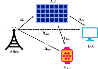
Figure 1: System model for RIS-assisted MISO wiretap channel.

Consider the MISO-RIS system shown in Fig. 1, consisting of a transmitter (Alice), one legitimate receiver (Bob), one eavesdropper (Eve), and one RIS. It is assumed that Alice is equipped with $N\geq 1$ antennas, while Bob and Eve are single-antenna devices. The RIS is assumed to have $N_{\mathrm{ris}}$ passive reflecting elements. The channel matrix between Alice and RIS is denoted by $\mathbf{H}_{ai}\in\mathbb{C}^{N_{\mathrm{ris}}\times N}$, while the channel vectors of Alice-Bob and Alice-Eve links are denoted by $\mathbf{h}_{ab}\in\mathbb{C}^{1\times N}$ and $\mathbf{h}_{ae}\in\mathbb{C}^{1\times N}$, respectively. The channel vectors of the RIS-Bob and RIS-Eve links are denoted by $\mathbf{h}_{ib}\in\mathbb{C}^{1\times N_{\mathrm{ris}}}$ and $\mathbf{h}_{ie}\in\mathbb{C}^{1\times N_{\mathrm{ris}}}$, respectively. Considering that Alice transmits a secret message $s\in\mathbb{C}$ intended for Bob, the signals received at Bob and Eve are, respectively, given by

$$y_{b} =\mathbf{h}_{ib}\operatorname{diag}\left(\boldsymbol{\theta}\right)\mathbf{H}_{ai}\mathbf{w}s+\mathbf{h}_{ab}\mathbf{w}s+n_{b},$$ (1)

$$y_{e} =\mathbf{h}_{ie}\operatorname{diag}\left(\boldsymbol{\theta}\right)\mathbf{H}_{ai}\mathbf{w}s+\mathbf{h}_{ae}\mathbf{w}s+n_{e},$$

where $\mathbf{w}\in\mathbb{C}^{N\times 1}$ is the transmit beamforming vector, $\boldsymbol{\theta}\triangleq\left[\theta_{1}\ \theta_{2}\ \cdots\ \theta_{N_{\mathrm{ris}}}\right]^{\mathsf{T}}\in\mathbb{C}^{N_{\mathrm{ris}}\times 1}$, $\theta_{l}=\exp\left(j\phi_{l}\right)$, $\phi_{l}\in\left[0,2\pi\right)$ denotes the phase shift induced by the $l$-th reflecting element in the RIS with $l\in\mathcal{L}$, $\mathcal{L}=\left\{1,2,\ldots,N_{\mathrm{ris}}\right\}$, and $n_{b}\sim\mathcal{CN}\left(0,\sigma_{b}^{2}\right)$ and $n_{e}\sim\mathcal{CN}\left(0,\sigma_{e}^{2}\right)$ denote the additive white Gaussian noise at Bob and Eve, respectively. Here we have $\left\|\mathbf{w}\right\|^{2}\leq P$, where $P$ denotes the maximum transmit power budget at Alice. Assuming that instantaneous CSI of all the wireless links are available at all nodes as well as the RIS, the ASR for Bob (in bps/Hz), for given $\mathbf{w}$ and $\boldsymbol{\theta}$, is given by

$$R_{s}\left(\mathbf{w},\boldsymbol{\theta}\right)=\log_{2}\left(\dfrac{1+\left|\mathbf{z}_{b}\left(\boldsymbol{\theta}\right)\mathbf{w}\right|^{2}}{1+\left|\mathbf{z}_{e}\left(\boldsymbol{\theta}\right)\mathbf{w}\right|^{2}}\right),$$ (2)

where $\mathbf{z}_{b}\left(\boldsymbol{\theta}\right)\triangleq\hat{\mathbf{h}}_{ib}\operatorname{diag}\left(\boldsymbol{\theta}\right)\mathbf{H}_{ai}+\hat{\mathbf{h}}_{ab}$, $\mathbf{z}_{e}\triangleq\hat{\mathbf{h}}_{ie}\operatorname{diag}\left(\boldsymbol{\theta}\right)\mathbf{H}_{ai}+\hat{\mathbf{h}}_{ae}$, $\hat{\mathbf{h}}_{ib}=\mathbf{h}_{ib}/\sigma_{b}$, $\hat{\mathbf{h}}_{ab}=\mathbf{h}_{ab}/\sigma_{b}$, $\hat{\mathbf{h}}_{ie}=\mathbf{h}_{ie}/\sigma_{e}$, and $\hat{\mathbf{h}}_{ae}=\mathbf{h}_{ae}/\sigma_{e}$.

We remark that the ASR is a useful performance metric for delay-tolerant applications. However, in this paper we are interested in the effective secrecy rate where some degree of QoS constraints must be satisfied. Let $\vartheta$ be the rate at which the buffer occupancy at Alice decays, where $\vartheta\triangleq-\lim_{x\to\infty}\tfrac{1}{x}\Pr\left\{\mathscr{L}>x\right\}$, with $\mathscr{L}$ being the queue length at equilibrium. Also, let $T$ denote the coherence time of all of the wireless links which is an integer multiple of the symbol duration and $\mathcal{B}$ denote the total available bandwidth. Since the channels are known to all the involving nodes, Alice can adapt the wiretap coding with respective to each channel realization to maximize the secrecy service rate. In this regard, the ESR for Bob (in bps/Hz) is defined as (c.f. [9, 10, eqn. (12)])

$$E_{s}\left(\mathbf{w},\boldsymbol{\theta}\right)\\ \triangleq\!\dfrac{-1}{\vartheta T\mathcal{B}}\ln\!\left(\!\mathbb{E}\left\{\exp\left(\!-\vartheta T\mathcal{B}\underset{\mathbf{w}\in\mathcal{S}_{w},\boldsymbol{\theta}\in\mathcal{S}_{\theta}}{\mathrm{max}\ }R_{s}\left(\mathbf{w},\boldsymbol{\theta}\right)\!\right)\!\right\}\!\right),$$ (3)

where the expectation is performed over the involved channels, and $\mathcal{S}_{w}$ and $\mathcal{S}_{\theta}$ are defined as

$$\mathcal{S}_{w} \triangleq\left\{\mathbf{w}\left|\left\|\mathbf{w}\right\|^{2}\leq P\right.\right\},$$ (4)

$$\mathcal{S}_{\theta} \triangleq\left\{\boldsymbol{\theta}\left|\left|\theta_{l}\right|=1,l\in\mathcal{L}\right.\right\}.$$

Note that $\vartheta\to 0$ represents the system without any delay constraint, whereas, $\vartheta\to\infty$ corresponds to the system with extremely-strict delay constraint. For the case when $\vartheta\to 0$, the ESR is identical to the ASR. It is obvious that to evaluate the effective secrecy rate, we need to solve the following optimization problem:

$$\underset{\mathbf{w},\boldsymbol{\theta}}{\operatorname{maximize}\ } f\left(\mathbf{w},\boldsymbol{\theta}\right)$$ (5)

$$\operatorname{subject~{}to} \mathbf{w}\in\mathcal{S}_{w},\ \boldsymbol{\theta}\in\mathcal{S}_{\theta}.$$

where

$$f\left(\mathbf{w},\boldsymbol{\theta}\right)\triangleq\dfrac{1+\left|\mathbf{z}_{b}\left(\boldsymbol{\theta}\right)\mathbf{w}\right|^{2}}{1+\left|\mathbf{z}_{e}\left(\boldsymbol{\theta}\right)\mathbf{w}\right|^{2}}.$$ (6)

It is not surprising that when channels are perfectly known at all nodes, finding the effective secrecy rate boils down to solving the conventional secrecy rate maximization problem. In the following section, we propose a method based on the concept of block coordinate ascent method to maximize the objective.

III Proposed Solution based on Block Coordinate Ascent Method

In this section, we present a computationally efficient algorithm to find a stationary solution to the problem in (5) that optimizes the beamforming vector $\mathbf{w}$ and each individual phase shift of the RIS using the BCAM. More specifically, we optimize $\mathbf{w}$ for a given $\boldsymbol{\theta}$, and optimize a specific phase shift $\theta_{l}$ for when $\mathbf{w}$ and other phase shifts $\theta_{m\neq l}$ are held fixed. These two steps are achieved in closed-forms as described in the next two subsections.

III-A Closed-Form Expression for Optimal $\mathbf{w}$ for Given $\boldsymbol{\theta}$

For a given phase shift vector $\boldsymbol{\theta},$ the optimization over $\mathbf{w}$ is expressed as

$$\operatorname{maximize} \dfrac{1+\mathbf{w}^{{\dagger}}\mathbf{Z}_{b}\left(\boldsymbol{\theta}\right)\mathbf{w}}{1+\mathbf{w}^{{\dagger}}\mathbf{Z}_{e}\left(\boldsymbol{\theta}\right)\mathbf{w}}$$ (7)

$$\operatorname{subject~{}to} \mathbf{w}\in\mathcal{S}_{w},$$

where $\mathbf{Z}_{b}\left(\boldsymbol{\theta}\right)\triangleq\mathbf{z}_{b}^{{\dagger}}\left(\boldsymbol{\theta}\right)\mathbf{z}_{b}\left(\boldsymbol{\theta}\right)$ and $\mathbf{Z}_{e}\left(\boldsymbol{\theta}\right)\triangleq\mathbf{z}_{e}^{{\dagger}}\left(\boldsymbol{\theta}\right)\mathbf{z}_{e}\left(\boldsymbol{\theta}\right)$, which admits a closed-form solution given by (c.f. [11])

$$\mathbf{w}_{\mathrm{opt}}=\sqrt{P}\mathbf{u}_{\max},$$ (8)

where $\mathbf{u}_{\max}$ is the normalized eigenvector associated with the maximum eigenvalue of the matrix $\left(P\mathbf{Z}_{e}\left(\boldsymbol{\theta}\right)+\mathbf{I}\right)^{-1}\left(P\mathbf{Z}_{b}\left(\boldsymbol{\theta}\right)+\mathbf{I}\right)$.

III-B Closed-Form Expression for Optimal $\theta_{l}$ for Given $\mathbf{w}$ and other $\theta_{m}\left(m\neq l\right)$

In this subsection, we derive a closed-form expression for optimal $\theta_{l}$ while other variables (including $\mathbf{w}$ and $\theta_{m}$, $m\in\left\{\mathcal{L}\setminus l\right\}$) are kept fixed. In fact, there are a few existing methods to find the phase shifts for a given $\mathbf{w}$. In [12], a combination of semi-definite rank relaxation method and Gaussian randomization was used. Yet, such a method incurs high complexity since a semi-definite program needs to be solved in each iteration. In [7], the authors applied Dinkelbach’s method together with the majorization-minimization principle to maximize a lower bound of $f\left(\mathbf{w},\boldsymbol{\theta}\right)$ in each iteration. The main drawback of this method is that a bisection search is still required, each iteration of which involves computing the maximum eigenvalue of a large matrix whose dimension is the number of reflecting elements (this value can be in the order of hundreds or even thousands in practically-envisioned RIS deployments).

Different from the existing solutions, our method can be viewed as a generalization of [13]. Note that the direct links for Alice-Bob and Alice-Eve channels were not considered in [13], and therefore it is not straightforward to adopt the solution proposed in [13]. Using the relation $\mathbf{x}\operatorname{diag}\left(\boldsymbol{\theta}\right)=\boldsymbol{\theta}^{\mathsf{T}}\operatorname{diag}\left(\mathbf{x}\right)$, we can further express the numerator of (7) as

$$1+\mathbf{w}^{{\dagger}}\mathbf{Z}_{b}\left(\boldsymbol{\theta}\right)\mathbf{w}$$

$$\!\!\mathcal{}\!=\ 1\!+\!\mathbf{w}^{{\dagger}}\!\left[\hat{\mathbf{h}}_{ib}\operatorname{diag}\left(\boldsymbol{\theta}\right)\mathbf{H}_{ai}\!+\!\hat{\mathbf{h}}_{ab}\right]^{{\dagger}}\!\left[\hat{\mathbf{h}}_{ib}\mathrm{\operatorname{diag}\left(\boldsymbol{\theta}\right)}\mathbf{H}_{ai}\!+\!\hat{\mathbf{h}}_{ab}\right]\mathbf{w}$$

$$\!\!\!\triangleq\ 1+\boldsymbol{\theta}^{{\dagger}}\mathbf{A}_{b}\left(\mathbf{w}\right)\boldsymbol{\theta}+\mathbf{b}_{b}^{{\dagger}}\left(\mathbf{w}\right)\boldsymbol{\theta}+\boldsymbol{\theta}^{{\dagger}}\mathbf{b}_{b}\left(\mathbf{w}\right)+c_{b}\left(\mathbf{w}\right),$$ (9)

where

$$\!\!\!\!\mathbf{A}_{b}\left(\mathbf{w}\right)\!=\!\mathbf{a}_{b}\left(\mathbf{w}\right)\mathbf{a}_{b}^{{\dagger}}\left(\mathbf{w}\right);\ \mathbf{\mathbf{a}}_{b}\left(\mathbf{w}\right)\!=\!\operatorname{diag}\left(\hat{\mathbf{h}}_{ib}^{*}\right)\mathbf{H}_{ai}^{*}\mathbf{w}^{*};$$ (10)

$$\!\!\!\!\mathbf{b}_{b}\left(\mathbf{w}\right)\!=\!\operatorname{diag}\left(\hat{\mathbf{h}}_{ib}^{*}\right)\mathbf{H}_{ai}^{*}\mathbf{w}^{*}\mathbf{w}^{\mathsf{T}}\hat{\mathbf{h}}_{ab}^{\mathsf{T}};\ c_{b}\left(\mathbf{w}\right)\!=\!\left|\hat{\mathbf{h}}_{ab}\mathbf{w}\right|^{2}.$$

Following a similar set of arguments, the denominator of (7) can be represented as

$$1+\mathbf{w}^{{\dagger}}\mathbf{Z}_{e}\left(\boldsymbol{\theta}\right)\mathbf{w}$$

$$=\ 1+\boldsymbol{\theta}^{{\dagger}}\mathbf{A}_{e}\left(\mathbf{w}\right)\boldsymbol{\theta}+\mathbf{b}_{e}^{{\dagger}}\left(\mathbf{w}\right)\boldsymbol{\theta}+\boldsymbol{\theta}^{{\dagger}}\mathbf{b}_{e}\left(\mathbf{w}\right)+c_{e}\left(\mathbf{w}\right),$$ (11)

where

$$\!\!\!\!\mathbf{A}_{e}\left(\mathbf{w}\right)\!=\!\mathbf{a}_{e}\left(\mathbf{w}\right)\mathbf{a}_{e}^{{\dagger}}\left(\mathbf{w}\right);\ \mathbf{\mathbf{a}}_{e}\left(\mathbf{w}\right)\!=\!\operatorname{diag}\left(\hat{\mathbf{h}}_{ie}^{*}\right)\mathbf{H}_{ai}^{*}\mathbf{w}^{*};$$ (12)

$$\!\!\!\!\mathbf{b}_{e}\left(\mathbf{w}\right)\!=\!\operatorname{diag}\left(\hat{\mathbf{h}}_{ie}^{*}\right)\mathbf{H}_{ai}^{*}\mathbf{w}^{*}\mathbf{w}^{\mathsf{T}}\hat{\mathbf{h}}_{ae}^{\mathsf{T}};\ c_{e}\left(\mathbf{w}\right)\!=\!\left|\hat{\mathbf{h}}_{ae}\mathbf{w}\right|^{2}.$$

Therefore, the optimization problem in (5) for a given $\mathbf{w}$ can be given by

$$\underset{\boldsymbol{\theta}}{\operatorname{maximize}\ } \dfrac{1+\boldsymbol{\theta}^{{\dagger}}\mathbf{A}_{b}\left(\mathbf{w}\right)\boldsymbol{\theta}+\mathbf{b}_{b}^{{\dagger}}\left(\mathbf{w}\right)\boldsymbol{\theta}+\boldsymbol{\theta}^{{\dagger}}\mathbf{b}_{b}\left(\mathbf{w}\right)+c_{b}\left(\mathbf{w}\right)}{1+\boldsymbol{\theta}^{{\dagger}}\mathbf{A}_{e}\left(\mathbf{w}\right)\boldsymbol{\theta}+\mathbf{b}_{e}^{{\dagger}}\left(\mathbf{w}\right)\boldsymbol{\theta}+\boldsymbol{\theta}^{{\dagger}}\mathbf{b}_{e}\left(\mathbf{w}\right)+c_{e}\left(\mathbf{w}\right)}$$ (13)

$$\operatorname{subject~{}to} \boldsymbol{\theta}\in\mathcal{S}_{\theta}.$$

To realize a more efficient method, we sequentially optimize each $\theta_{l}$ at a time while the other phase shifts (along with the other variables) are held fixed. To lighten the notations, we write $\mathbf{A}_{b}$ instead of $\mathbf{A}_{b}\left(\mathbf{w}\right)$ onward. The same applies to other quantities in (10) and the quantities in (12). Let $\mathbf{a}_{b}=\left[a_{b1}\ a_{b2}\ \cdots\ a_{bN_{\mathrm{ris}}}\right]^{\mathsf{T}}$, $\mathbf{a}_{e}=\left[a_{e1}\ a_{e2}\ \cdots\ a_{eN_{\mathrm{ris}}}\right]^{\mathsf{T}}$, $\mathbf{b}_{b}=\left[b_{b1}\ b_{b2}\ \cdots\ b_{bN_{\mathrm{ris}}}\right]^{\mathsf{T}}$ and $\mathbf{b}_{e}=\left[b_{e1}\ b_{e2}\ \cdots\ b_{eN_{\mathrm{ris}}}\right]^{\mathsf{T}}$. Then the maximization over a specific $\theta_{l}$ is expressed as

$$\underset{\theta_{l}}{\operatorname{maximize}} \dfrac{\Re\left\{\alpha_{bl}^{*}\theta_{l}\right\}+\beta_{bl}}{\Re\left\{\alpha_{el}^{*}\theta_{l}\right\}+\beta_{el}}$$ (14)

$$\operatorname{subject~{}to} \left|\theta_{l}\right|=1,$$

where $\alpha_{bl}=2\left(a_{bl}\sum\nolimits_{m\in\left\{\mathcal{L}\setminus l\right\}}a_{bm}^{*}\theta_{m}+b_{bl}\right),$ $\beta_{bl}=\left|a_{bl}\right|^{2}+\left|\sum\nolimits_{m\in\left\{\mathcal{L}\setminus l\right\}}a_{bm}^{\ast}\theta_{m}\right|^{2}+2\Re\left\{\sum\nolimits_{m\in\left\{\mathcal{L}\setminus l\right\}}b_{bm}^{\ast}\theta_{m}\right\}+c_{b}+1$, $\alpha_{el}=2\left(a_{el}\sum\nolimits_{m\in\left\{\mathcal{L}\setminus l\right\}}a_{em}^{*}\theta_{m}+b_{el}\right)$ and $\beta_{el}=\left|a_{el}\right|^{2}+\left|\sum\nolimits_{m\in\left\{\mathcal{L}\setminus l\right\}}a_{em}^{\ast}\theta_{m}\right|^{2}+2\Re\left\{\sum\nolimits_{m\in\left\{\mathcal{L}\setminus l\right\}}b_{em}^{\ast}\theta_{m}\right\}+c_{e}+1$. To proceed further, we rewrite $\alpha_{bl}=r_{bl}\exp\left(j\phi_{bl}\right)$, $\alpha_{el}=r_{el}\exp\left(j\phi_{el}\right)$ and $\theta_{l}=\exp\left(j\phi_{l}\right)$. Then, (14) reduces to

$$\underset{\phi_{l}}{\operatorname{maximize}} \dfrac{r_{bl}\cos\left(\phi_{l}-\phi_{bl}\right)+\beta_{bl}}{r_{el}\cos\left(\phi_{l}-\phi_{el}\right)+\beta_{el}}\triangleq g\left(\phi_{l}\right)$$ (15)

$$\operatorname{subject~{}to} 0\leq\phi_{l}<2\pi.$$

Differentiating the objective function in (15) w.r.t. $\phi_{l}$, we get

$$g^{\prime}\left(\phi_{l}\right)=\dfrac{-r_{bl}\sin\left(\phi_{l}-\phi_{bl}\right)\left\{r_{el}\cos\left(\phi_{l}-\phi_{el}\right)+\beta_{el}\right\}}{\left\{r_{el}\cos\left(\phi_{l}-\phi_{el}\right)+\beta_{el}\right\}^{2}}$$

$$\qquad\qquad+\dfrac{r_{el}\sin\left(\phi_{l}-\phi_{el}\right)\left\{r_{bl}\cos\left(\phi_{l}-\phi_{bl}\right)+\beta_{bl}\right\}}{\left\{r_{el}\cos\left(\phi_{l}-\phi_{el}\right)+\beta_{el}\right\}^{2}}$$

$$=\!\frac{r_{bl}r_{el}\sin\left(\!\phi_{bl}\!-\!\phi_{el}\!\right)\!+\!r_{el}\beta_{bl}\sin\left(\!\phi_{l}\!-\!\phi_{el}\!\right)\!-\!r_{bl}\beta_{el}\sin\left(\!\phi_{l}\!-\!\phi_{bl}\!\right)}{\left\{r_{el}\cos\left(\phi_{l}-\phi_{el}\right)+\beta_{el}\right\}^{2}}.$$ (16)

Using the following relation,

$$r_{bl}\beta_{el}\sin\left(\phi_{l}-\phi_{bl}\right)-r_{el}\beta_{bl}\sin\left(\phi_{l}-\phi_{el}\right)=r_{l}\sin\left(\phi_{l}+\varphi_{l}\right),$$

where

$$r_{l}= \sqrt{r_{bl}^{2}\beta_{el}^{2}+r_{el}^{2}\beta_{bl}^{2}-2r_{bl}r_{el}\beta_{bl}\beta_{el}\cos\left(\phi_{el}-\phi_{bl}\right)},$$

$$\varphi_{l}= \arctan\left[\dfrac{-r_{bl}\beta_{el}\sin\left(\phi_{bl}\right)+r_{el}\beta_{bl}\sin\left(\phi_{el}\right)}{r_{bl}\beta_{el}\cos\left(\phi_{bl}\right)-r_{el}\beta_{bl}\cos\left(\phi_{el}\right)}\right],$$

we can rewrite $g^{\prime}\left(\phi_{l}\right)$ as

$$g^{\prime}\left(\phi_{l}\right)=\dfrac{r_{bl}r_{el}\sin\left(\phi_{bl}-\phi_{el}\right)-r_{l}\sin\left(\phi_{l}+\varphi_{l}\right)}{\left\{r_{el}\cos\left(\phi_{l}-\phi_{el}\right)+\beta_{el}\right\}^{2}}.$$ (17)

Note that if $\left|r_{bl}r_{el}\sin\left(\phi_{bl}-\phi_{el}\right)\right|>r_{l}$, then $g^{\prime}\left(\phi_{l}\right)$ is either positive or negative (i.e., $g^{\prime}\left(\phi_{l}\right)$ can not be equal to zero) for all $\phi_{l}\in\left[0,2\pi\right)$. As a result, $g(\phi_{l})$ is maximized when $\phi_{l}=0$, resulting in $\theta_{l}=1$. On the other hand, if $\left|r_{bl}r_{el}\sin\left(\phi_{bl}-\phi_{el}\right)\right|\leq r_{l}$, then $g^{\prime}\left(\phi_{l}\right)=0$ has two solutions:

$$\phi_{l_{1}} =\arcsin\left[\tfrac{r_{bl}r_{el}}{r_{l}}\sin\left(\phi_{bl}-\phi_{el}\right)\right]-\varphi_{l},$$ (18)

$$\phi_{l_{2}} =\pi-\arcsin\left[\tfrac{r_{bl}r_{el}}{r_{l}}\sin\left(\phi_{bl}-\phi_{el}\right)\right]-\varphi_{l}.$$

Thus the optimal solution to (14) admits a closed-form expression given by

$$\theta_{l,\mathrm{opt}}=\exp\left(j\phi_{l,\mathrm{opt}}\right),$$ (19)

where

$$\phi_{l,\mathrm{opt}}=\operatorname{argmax}\left\{g\left(0\right),g\left(\phi_{l_{1}}\right),g\left(\phi_{l_{2}}\right)\right\},$$ (20)

and $\phi_{l_{1}}$ and $\phi_{l_{2}}$ are given in (18). The overall algorithm is summarized in Algorithm 1.

1

2

Input: $\boldsymbol{\theta}_{0}$, $\mathbf{w}_{0}$

3

Output: $\boldsymbol{\theta}_{n},\mathbf{w}_{n}$

4

5$n\leftarrow 1$;

6

7repeat

8      

9      Given $\boldsymbol{\theta}_{n-1}$, compute $\mathbf{w}_{n}$ via (8)

10      for $l\in\mathcal{L}$ do

11            

12            Compute $\theta_{l,\mathrm{opt}}$ for given $\mathbf{w}_{n}$ via (19)

13            $\theta_{l}\leftarrow\theta_{l,\mathrm{opt}}$

14       end for

15      

16      $n\leftarrow n+1$

17until convergence ;

Algorithm 1 Block Coordinate Ascent Method

III-C Convergence Analysis

We now show that the iterates generated by Algorithm 1 converge to a stationary solution of (5). First, it is easy to see that $f(\mathbf{w}_{n+1},\boldsymbol{\theta}_{n+1})\geq f(\mathbf{w}_{n+1},\boldsymbol{\theta}_{n})\geq f(\mathbf{w}_{n},\boldsymbol{\theta}_{n})$ and thus Algorithm 1 generates a non-decreasing objective sequence. It is also trivial to check that the objective function is continuous and bounded from above. Moreover, the feasible set is compact. Thus, the objective sequence must converge to certain limit, i.e., $\underset{n\to\infty}{\lim}f(\mathbf{w}_{n},\boldsymbol{\theta}_{n})=f_{\ast}$. Let $\mathcal{S}=\{(\mathbf{w},\boldsymbol{\theta})\ |\ f(\mathbf{w},\boldsymbol{\theta})\leq f_{\ast}\}$. By the continuity of $f(\mathbf{w},\boldsymbol{\theta})$ and the compactness of the feasible set, it is obvious that $\mathcal{S}$ is compact. Thus there exists a subsequence $(\mathbf{w}_{n_{j}},\boldsymbol{\theta}_{n_{j}})$ converging to the limit point $(\mathbf{w}_{\ast},\boldsymbol{\theta}_{\ast})$. By continuity of $f(\mathbf{w},\boldsymbol{\theta})$ we must have $f_{\ast}=f(\mathbf{w}_{\ast},\boldsymbol{\theta}_{\ast})$. The proof that $(\mathbf{w}_{\ast},\boldsymbol{\theta}_{\ast})$ is a stationary solution of (5) is rather standard and thus is omitted here for the sake of brevity. We refer the interested reader to [14, Sec. 2.7] for further details.

III-D Efficient Implementation and Complexity Analysis

We now provide an efficient implementation and the associated complexity analysis of the proposed solution. For the complexity analysis, we use the conventional big-O notation and focus on the number of complex multiplications. First, note that $P\mathbf{Z}_{b}\left(\boldsymbol{\theta}\right)$ can be represented as $\left(P\mathbf{z}_{b}\left(\boldsymbol{\theta}\right)\right)^{{\dagger}}\mathbf{z}_{b}\left(\boldsymbol{\theta}\right)$. The number of multiplications required to compute $P\mathbf{z}_{b}\left(\boldsymbol{\theta}\right)$ is equal to $\mathcal{O}\left(NN_{\mathrm{ris}}\right)$ and the number of multiplications required to compute $P\mathbf{Z}_{b}\left(\boldsymbol{\theta}\right)$ is given by $N^{2}/2$. Note that the $\mathbf{w}$-update requires the eigenvector associated with the maximum eigenvalue of $\bigl{(}P\mathbf{Z}_{e}\left(\boldsymbol{\theta}\right)+\mathbf{I}\bigr{)}^{-1}\bigl{(}P\mathbf{Z}_{b}\left(\boldsymbol{\theta}\right)+\mathbf{I}\bigr{)}$. If we compute this term in a straightforward manner, it would take $\mathcal{O}\left(N^{3}\right)$ complex multiplications. We now provide an efficient way to achieve this, which has not been discussed in the related literature. Using the Woodbury matrix identity [15], it can be shown that $P\mathbf{Z}_{e}\left(\boldsymbol{\theta}\right)+\mathbf{I}\bigr{)}^{-1}=\mathbf{I}-\tfrac{P\mathbf{z}_{e}\left(\boldsymbol{\theta}\right)^{{\dagger}}\mathbf{z}_{e}\left(\boldsymbol{\theta}\right)}{1+P\mathbf{z}_{e}\left(\boldsymbol{\theta}\right)\mathbf{z}_{e}^{{\dagger}}\left(\boldsymbol{\theta}\right)}$. Therefore, we have

$$\bigl{(}P\mathbf{Z}_{e}\left(\boldsymbol{\theta}\right)+\mathbf{I}\bigr{)}^{-1}\bigl{(}P\mathbf{Z}_{b}\left(\boldsymbol{\theta}\right)+\mathbf{I}\bigr{)}$$

$$=\ \mathbf{I}+P\mathbf{Z}_{b}\left(\boldsymbol{\theta}\right)-\dfrac{P^{2}\mathbf{z}_{e}\left(\boldsymbol{\theta}\right)^{{\dagger}}\mathbf{z}_{e}\left(\boldsymbol{\theta}\right)\mathbf{z}_{b}^{{\dagger}}\left(\boldsymbol{\theta}\right)\mathbf{z}_{b}\left(\boldsymbol{\theta}\right)}{1+P\mathbf{z}_{e}\left(\boldsymbol{\theta}\right)\mathbf{z}_{e}^{{\dagger}}\left(\boldsymbol{\theta}\right)}.$$

Note that the terms $\mathbf{z}_{e}\left(\boldsymbol{\theta}\right)\mathbf{z}_{e}^{{\dagger}}\left(\boldsymbol{\theta}\right)$ in the denominator and $\mathbf{z}_{e}\left(\boldsymbol{\theta}\right)\mathbf{z}_{b}^{{\dagger}}\left(\boldsymbol{\theta}\right)$ in the numerator are scalars; both require $N$ complex multiplications, whereas the term $\mathbf{z}_{e}\left(\boldsymbol{\theta}\right)^{{\dagger}}\mathbf{z}_{b}\left(\boldsymbol{\theta}\right)$ in the numerator needs $\mathcal{O}\left(N^{2}\right)$ complex multiplications. Therefore, the complexity to compute $\left(P\mathbf{Z}_{e}\left(\boldsymbol{\theta}\right)+\mathbf{I}\right)^{-1}\left(P\mathbf{Z}_{b}\left(\boldsymbol{\theta}\right)+\mathbf{I}\right)$ is $\mathcal{O}\left(N^{2}\right)$. Reducing the complexity for computing $\left(P\mathbf{Z}_{e}\left(\boldsymbol{\theta}\right)+\mathbf{I}\right)^{-1}\left(P\mathbf{Z}_{b}\left(\boldsymbol{\theta}\right)+\mathbf{I}\right)$ from $\mathcal{O}\left(N^{3}\right)$ to $\mathcal{O}\left(N^{2}\right)$ is particularly helpful for the case of extra-large MISO system where the number of transmit antennas at Alice is very large. Moreover, to find $\mathbf{u}_{\max}$, we need $\mathcal{O}\left(N^{3}\right)$ complex multiplications. Therefore, the overall complexity for each update of $\mathbf{w}_{n}$ is given by $\mathcal{O}\left(NN_{\mathrm{ris}}+\tfrac{N^{2}}{2}+N^{2}+N^{3}\right)=\mathcal{O}\left(N^{3}+NN_{\mathrm{ris}}\right)$. Following a similar line of argument, it can be noted that the number of multiplications required to compute $\alpha_{bl}$, $\beta_{bl}$, $\alpha_{el}$, and $\beta_{el}$ are all $\mathcal{O}\left(N_{\mathrm{ris}}\right)$. Therefore, the complexity associated to update all phase shifts is given by $\mathcal{O}\left(N_{\mathrm{ris}}^{2}\right)$. Hence, it can be concluded that the overall complexity associated with each iteration of Algorithm 1 (see lines 3–8) is given by $\mathcal{O}\left(N^{3}+NN_{\mathrm{ris}}+N_{\mathrm{ris}}^{2}\right)$.

IV Simulation Results and Discussion

In this section, we present the simulation results for the ESR for the MISO-RIS system. In order to facilitate a fair comparison with a benchmark scheme, we consider the same system parameters as used in [7]. For all of the wireless links, the small-scale fading is modeled as Rayleigh distributed, whereas, the path loss model is given by $\mathrm{PL}=\left[\mathrm{PL_{ref}}-10\xi\log_{10}\left(d/d_{\mathrm{ref}}\right)\right]$ dB. Here, $\mathrm{PL_{ref}}$ denotes the path loss at the reference distance $d_{\mathrm{ref}}$, $\xi$ is the path loss exponent, and $d$ is the distance between transmitter and receiver. The values of different system parameters are given in Table I. In Fig. 2, the ESR is plotted for 50 different channel realizations, whereas, in Figs. 3–5, the ESR is plotted for $10^{3}$ different channel realizations.

TABLE I: System parameter values [7].

System Parameter	Value
Transmit power, $P$	15 dBW
Noise power, $\sigma_{b}^{2}=\sigma_{e}^{2}$	-75 dBW
Reference distance, $d_{\mathrm{ref}}$	1 m
Path loss at reference distance, $\mathrm{PL_{ref}}$	-30 dBW
Path loss exponent for Alice-RIS links, $\xi_{ai}$	2.2
Path loss exponent for RIS-Bob links, $\xi_{ib}$	2.5
Path loss exponent for RIS-Eve links, $\xi_{ie}$	2.5
Path loss exponent for Alice-Bob links, $\xi_{ab}$	3.5
Path loss exponent for Alice-Eve links, $\xi_{ae}$	3.5
Alice-RIS distance, $d_{ai}$	50 m
Alice-Eve horizontal distance, $d_{ae,h}$	44 m
Alice-Bob horizontal distance (in meters)	$d_{ab,h}$
Vertical distance between the line joining	2 m
Alice and RIS, and Bob and Eve, i.e., $d_{v}$

Figure 2: Convergence of ESR for $\vartheta\to 0$ and $d_{ab,h}=10$ m.

Fig. 2 shows a comparison of the speed of convergence between the proposed method (BCAM) and the bisection-search-based AO given in [7]. Here one iteration constitutes one update of the beamforming vector and one update of the phase shift vector (see lines 3–8 in Algorithm 1), which is consistent with one iteration of the method in [7], and thus the comparison is fair. It is clear from the figure that the proposed method converges significantly faster than that of the algorithm adopted in [7], establishing the superiority of the proposed algorithm.

Figure 3: The variation in ESR versus the horizontal distance between Alice and Bob for $N=4,N_{\mathrm{ris}}=32$ and different values of delay QoS exponent.

Figure 4: The variation of ESR versus the delay exponent $\vartheta$ for $N_{\mathrm{ris}}=32$, $d_{ab,h}=40$ m and different values of $N$.

Figure 5: The variation of ESR versus $N_{\mathrm{ris}}$ for $N=4$, $d_{ab,h}=40$ m and different values of $\vartheta$.

Fig. 3 shows the variation in ESR versus the horizontal distance between Alice and Bob (denoted by $d_{ab,h}$). Note that for the system without any delay constraints (i.e., $\vartheta\to 0$), the ESR becomes equal to the ASR. It is evident from the figure that as the delay requirement of the system becomes more stringent, i.e., for larger values of $\vartheta$, the ESR of the MISO-RIS system decreases significantly. It can also be noted from the figure that as the horizontal distance between Alice and Bob increases, the ESR of the system decreases, because the Alice-Bob links becomes weak. However, when $d_{ab,h}\in\left[40,50\right]$ m, the distance between RIS and Bob becomes very small, and therefore, the RIS-Bob links become very strong, resulting in an increased ESR. Moreover, the superiority of introducing RIS is also clearly evident from the figure, as the ones with RIS result in a significantly higher ESR than those without RIS, for which the ESR decreases monotonically with increasing value of $d_{ab,h}$.

In Fig. 4, we show the effect of increasing delay QoS exponent on the ESR for different number of transmit antennas. It is clear from the figure that as the delay constraints for the system becomes more strict, the ESR decreases. As expected, the RIS-assisted system outperforms its counterpart without RIS. More interestingly, for the case when Alice is equipped with a single transmit antenna $\left(N=1\right)$, the system exhibits very poor ESR. However, as the number of transmit antennas at Alice increases, sharp energy-focused beamforming can performed at Alice to enhance the secrecy rate performance. It is also noteworthy that increasing the value of $N$ results in diminishing returns.

Fig. 5 shows the variation in the ESR w.r.t. $N_{\mathrm{ris}}$ for different values of the delay QoS exponent $\vartheta$. The performance superiority of the RIS-assisted system over the ones without RIS is clearly evident from the figure. More interestingly, it can be noted from the figure that for an exponential increase in the number of reflecting elements at RIS, i.e., $N_{\mathrm{ris}}$, the ESR increases exponentially. Moreover, it is also interesting to note that as the value of $N_{\mathrm{ris}}$ increases, the difference between the ESR of the RIS-assisted system with different $\vartheta$ values decreases. This occurs due to the fact that for a very large value of $N_{\mathrm{ris}}$, the fluctuation in the term $R_{s}$$\left(\mathbf{w},\boldsymbol{\theta}\right)$ in (3) becomes very less, and therefore, the effect of the delay QoS exponent $\vartheta$ on the ESR becomes negligible. This result indicates that a large number of reflecting elements in the RIS helps reducing the degradation in the ESR for delay-constrained systems.

V Conclusion

In this paper, we considered the problem of maximizing the secrecy rate of a MISO-RIS system subject to the total transmit power constraint and the delay-limited QoS constraint. We proposed a block coordinate ascent method to find closed-form expressions for the beamformer and the phase shift vector to maximize the objective. The convergence superiority of the proposed solution over the bisection-search-based AO is confirmed via Monte-Carlo simulation. The simulation results confirmed that the secrecy rate of the system under stringent delay requirements is significantly lower than the achievable secrecy rate, however, a large-size RIS can greatly enhance the secrecy rate performance of the system under delay constraints. Our results also confirm that the ESR of the MISO-RIS system increases with an increase in the number of transmit antennas and/or the number of reflecting elements at the RIS.

References

• [1] Q. Wu and R. Zhang, “Towards smart and reconfigurable environment: Intelligent reflecting surface aided wireless network,” IEEE Commun. Mag., vol. 58, no. 1, pp. 106–112, Jan. 2020.
• [2] A. Almohamad, A. M. Tahir, A. Al-Kababji, H. M. Furqan, T. Khattab, M. O. Hasna, and H. Arslan, “Smart and secure wireless communications via reflecting intelligent surfaces: A short survey,” IEEE Open J. Commun. Soc., vol. 1, pp. 1442–1456, Sep. 2020.
• [3] X. Guan, Q. Wu, and R. Zhang, “Intelligent reflecting surface assisted secrecy communication: Is artificial noise helpful or not?” IEEE Wireless Commun. Lett., vol. 9, no. 6, pp. 778–782, Jan. 2020.
• [4] H.-M. Wang, J. Bai, and L. Dong, “Intelligent reflecting surfaces assisted secure transmission without eavesdropper’s CSI,” IEEE Signal Process. Lett., vol. 27, pp. 1300–1304, Jul. 2020.
• [5] X. Lu, W. Yang, X. Guan, Q. Wu, and Y. Cai, “Robust and secure beamforming for intelligent reflecting surface aided mmWave MISO systems,” IEEE Wireless Commun. Lett., vol. 9, no. 12, pp. 2068–2072, Jul. 2020.
• [6] L. Dong and H.-M. Wang, “Secure MIMO transmission via intelligent reflecting surface,” IEEE Wireless Commun. Lett., vol. 9, no. 6, pp. 787–790, Jan. 2020.
• [7] H. Shen, W. Xu, S. Gong, Z. He, and C. Zhao, “Secrecy rate maximization for intelligent reflecting surface assisted multi-antenna communications,” IEEE Commun. Lett., vol. 23, no. 9, pp. 1488–1492, Jun. 2019.
• [8] D. Wu and R. Negi, “Effective capacity: A wireless link model for support of quality of service,” IEEE Trans. Wireless Commun., vol. 2, no. 4, pp. 630–643, Jul. 2003.
• [9] W. Yu, A. Chorti, L. Musavian, H. Vincent Poor, and Q. Ni, “Effective secrecy rate for a downlink NOMA network,” IEEE Trans. Wireless Commun., vol. 18, no. 12, pp. 5673–5690, Sep. 2019.
• [10] M. C. Gursoy, “MIMO wireless communications under statistical queueing constraints,” IEEE Trans. Inf. Theory, vol. 57, no. 9, pp. 5897–5917, Aug. 2011.
• [11] A. Khisti and G. W. Wornell, “Secure transmission with multiple antennas I: The MISOME wiretap channel,” IEEE Trans. Inf. Theory, vol. 56, no. 7, pp. 3088–3104, Jun. 2010.
• [12] M. Cui, G. Zhang, and R. Zhang, “Secure wireless communication via intelligent reflecting surface,” IEEE Wireless Commun. Lett., vol. 8, no. 5, pp. 1410–1414, May 2019.
• [13] X. Yu, D. Xu, and R. Schober, “Enabling secure wireless communications via intelligent reflecting surfaces,” in IEEE Global Commun. Conf. (GLOBECOM), 2019, pp. 1–6.
• [14] D. Bertsekas, Nonlinear Programming.   Athena Scientific, 1999.
• [15] M. A. Woodbury, Inverting modified matrices.   Statistical Research Group, 1950.