Statistical Inference from Partially Nominated Sets: An Application to Estimating the Prevalence of Osteoporosis Among Adult Women

Abstract

This paper focuses on drawing statistical inference based on a novel variant of maxima or minima nomination sampling (NS) designs. These sampling designs are useful for obtaining more representative sample units from the tails of the population distribution using the available auxiliary ranking information. However, one common difficulty in performing NS in practice is that the researcher cannot obtain a nominated sample unless he/she uniquely determines the sample unit with the highest or the lowest rank in each set. To overcome this problem, a variant of NS which is called partial nomination sampling is proposed in which the researcher is allowed to declare that two or more units are tied in the ranks whenever he/she cannot find with high confidence the sample unit with the highest or the lowest rank with high confidence. Based on this sampling design, two asymptotically unbiased estimators are developed for the cumulative distribution function, which are obtained using maximum likelihood and moment-based approaches, and their asymptotic normality is proved. Several numerical studies have shown that the developed estimators have higher relative efficiencies than their counterpart in simple random sampling in analyzing either the upper or the lower tail of the parent distribution. The procedures that we are developed are then implemented on a real dataset from the Third National Health and Nutrition Examination Survey (NHANES III) to estimate the prevalence of osteoporosis among adult women aged 50 and over. It is shown that in some certain circumstances, the techniques that we have developed require only one-third of the sample size needed in SRS to achieve the desired precision. This results in a considerable reduction of time and cost compared to the standard SRS method.

Keywords: imperfect ranking; ranked set sampling; maximum likelihood; nonparametric estimation; relative efficiency; tie information

Mathematics Subject Classifications (2020): Primary: 62D05; Secondary: 92B15

Department of Statistics, Faculty of Mathematics and Statistics, University of Isfahan,

Isfahan 81746-73441, Iran

1 Introduction

In some medical applications such as survival analysis, cancer studies, risk analysis, and prevalence studies, the researcher is interested in drawing a statistical inference about either the lower or the upper tail of the population distribution. For instance, in large cohort studies on measuring bone mineral density (BMD) among elderly women in a given population, the researcher is often interested in the lower quantile of the population since the lower values of BMD are related to a higher possibility of bone fracture due to some minor incidents such as falls or sport injuries. This imposes a substantial financial burden on the society due to the high cost of medical treatment and the possibility of the patients’ lifetime disability.

In situations where the researcher is only interested in either the upper or the lower tail of the population distribution, the usual simple random sampling (SRS) design might not lead to a good representative sample since enough units from the tails of the distribution may not be included in the sample. On the other hand, when measuring the actual value of the variable of interest is time-consuming, expensive, or hazardous, a large enough SRS sample may not be available to guarantee that the resulting sample captures all aspects of the given population related to at least one of the tails of the distribution. There is sometimes a wealth of auxiliary information about the population of interest which cannot be translated into covariates. Nevertheless, they can be used by some more structured sampling designs such as nomination sampling (NS) to select a more representative sample from the tails of population as is possible in SRS. For instance, assume that a medical researcher is interested in obtaining the prevalence of women with a BMD lower than a given threshold in a certain population. Note that measuring a person’s actual BMD is an expensive and time-consuming job because it requires Dual-energy X-ray absorptiometry (DXA) technology which is expensive and not easily accessible in developing countries. In addition, it is inconvenient since it needs a medical expert to segment the pertinent images manually. However, a medic can first use his/her past experience to nominate the patients who are more likely to have the lowest BMD values among the others for further consideration and then the actual BMD values of the nominated sample units can be obtained via DXA technology. As has been shown in the literature (for example, see Zamanzade and Mahdizadeh, 2020), the use of NS rather than SRS can lead to a considerable efficiency gain at either the lower or the upper tail of the distribution. As a result, a substantial reduction in time and cost will be achieved for a predefined precision.

The NS technique was first suggested by Willemain (1980) in his effort to develop a more acceptable way to pay for nursing home services. He argued that nursing home service operators would be reluctant to accept sample-based reimbursement rate by the government unless they were allowed to play a role in the sampling process. In particular, the operators might be allowed to include those residents with the highest caring costs in the sample. Hence, the cited author introduced NS to draw a statistical inference based on such samples. This sampling strategy is also the only practical option when historical data include only extreme values (Willemain, 1980). NS has been used for estimating the population median (Willemain, 1980), the cumulative distribution function (CDF) (Boyles and Samaniego, 1986), constructing acceptance sampling plans (Jafari Jozani and Mirkamali, 2010), and the quality control charts (Jafari Jozani and Mirkamali, 2011), quantile estimation (Nourmohammadi et al., 2014) and quantile regression (Jafari Jozani et al., 2018).

NS can be regarded as a special case of ranked set sampling (RSS) proposed by McIntyre (1952) as an efficient method for estimating pasture yields in Australia. RSS is applicable in situations where the sample units in a small-sized set can be easily ranked without referring to their actual values. These situations may occur in environmental, ecological, biological, medical, and fisheries studies. In fact, the sample units in RSS are obtained based on additional information from some unquantified units in terms of judgment ranks in order to provide a more structured sample from the population of interest. Since its introduction, RSS has been the subject of many studies and virtually all standard statistical problems using RSS have been addressed in the literature. These include, among others, the estimation of the population mean (Takahasi and Wakitomo, 1968; Ozturk, 2011; Frey, 2012; Frey and Feeman, 2016), the CDF (Stokes and Sager, 1988; Samawi and Al-Sagheer, 2001; Duembgen and Zamanzade, 2020), the population proportion (Chen et al., 2005; Zamanzade and Mahdizadeh, 2017; Omidvar et al., 2018; Frey and Zhang, 2019, 2021), perfect ranking tests (Frey et al., 2007; Frey and Zhang, 2017; Frey and Wang, 2013, 2014), odds ratio (Samawi and Al-Saleh, 2013), logistic regression (Samawi and Al-Saleh, 2013; Samawi et al., 2017, 2018; Samawi-sample-2020), the Youden index (Samawi et al., 2017), parameter estimation (Chen et al., 2018, 2019; He et al., 2020, 2021; Qian et al., 2021), randomized cluster design (Ahn et al., 2017; Wang et al., 2016, 2017, 2020) and statistical control quality charts (Al-Omari and Haq, 2011; Haq et al., 2013; Haq and Al-Omari, 2014; Haq et al., 2014).

In the NS design, a sample unit with the highest/lowest judgment rank in a small-sized set has to be determined uniquely by the researcher. In this paper, a new variant of NS called ‘partial nomination sampling (PNS) design’ is developed in which the researcher is allowed to declare ties whenever he/she cannot find with high confidence the sample unit with the highest/lowest rank. In Section 2, PNS is described in detail and its usage is shown by a hypothetical example. In Section 3, two estimators of the CDF are developed and their asymptotic normality is proved. In Section 4, the estimators that we developed are compared with their SRS counterpart. A real dataset is analyzed in Section 5 to show the applicability of our proposed procedure in the current paper. Some concluding remarks and directions for future research are provided in Section 6.

2 Sampling design set up

Let $m$ be the set size. The NS proposed by Willemain (1980) is a two-step sampling method. In the first step, the researcher is required to draw $n$ simple random samples (each with the size of $m$) from an infinite population and then rank each sample with the size of $m$ from the smallest to the largest with respect to the variable of interest using any relatively cheap and convenient method which does not entail the actual quantification of the sample units. In the second step, the researcher draws one unit with the smallest/largest rank from each set for exact measurement. Therefore, this process can be outlined as follows:

1. Determine an integer value for the size of the set $\left(m\right)$. In order to facilitate the ranking process, the value of $m$ should be kept small (e.g. from 2 to 10).

2. Identify $n\times m$ units from the target population and partition them randomly into $n$ sets each with the size of $m$. Then, rank each set with the size of $m$ from the smallest to the largest. The ranking process in this step is done without any reference to the actual values of the set units. Therefore, it is prone to error (imperfect).

3. Select the sample unit with the smallest rank in each set with the size of $m$ for actual measurement.

The above sampling design is called ‘MinNS’ and the sample units are denoted by $\left\{Y_{\left[1\right]i},i=1,\ldots n\right\},$ where $Y_{\left[1\right]i}$ denotes the sample unit with the smallest judgment rank in the $i$-th set. In the third step mentioned above, the sample unit with the highest judgment rank in each set with the size of $m$ is selected for actual measurement. In this case, the sampling design is called ‘MaxNS’ and the resulting sample units are denoted by $\left\{Y_{\left[m\right]i},i=1,\ldots n\right\},$ where $Y_{\left[m\right]i}$ denotes the sample unit with the highest judgment rank in the $i$-th set. There are two main difficulties in performing NS in practice which are both rooted in the nature of the ranking process since it is done without any reference to the actual values of the sample units. The first one is called ‘imperfect ranking’ which refers to situations in which the sample unit with the lowest (highest) judgment rank in the set with the size of $m$ may not be the same as the sample unit with the true lowest (highest) rank in the set. Therefore, it is essential to show that the developed procedures based on the NS design are relatively robust for imperfect ranking as long as the quality of ranking is fairly good. The second hardship in applying NS in real situations is about the ties in the ranking process which pertains to situations in which the researcher cannot determine with high confidence the sample unit with the lowest (highest) judgment rank in the set with the size of $m$ and therefore two or more units in the set are tied as the lowest (highest) rank. The current solution for this problem is to ignore the information of the ties and select one of the tied units at random for actual quantification. In this paper, not only breaking the ties at random in NS but also recording their information for use in the estimation process are proposed. The outline of the proposed sampling method is given below:

1. Denote by $\mathbf{I}$, the matrix of the ties information with $n$ rows and $m$ columns, where $m$ is the size of the set and $n$ is the sample size.

2. Similar to NS, identify $n\times m$ units from the target population and randomly partition them into $n$ sets each with the size of $m$ and then rank each set from the smallest to the largest.

3. From the $i$-th set, select the sample unit with the lowest judgment rank (for $i=1,\ldots,n$). Define $I_{i,j}=1$, if the researcher cannot distinguish between the sample unit with the lowest judgment rank in the $i$-th set and the sample unit with the judgment rank $j$ in the same set. Otherwise, $I_{i,j}=0$, where $I_{i,j}$ is the element in the $i$-th row and $j$-th column of the matrix of the ties information $\mathbf{I}$.

The above sampling plan is called ‘MinPNS’ and the sample units include not only the measured values of $\left\{Y_{\left[1\right]i},i=1,\ldots n\right\},$ but also the matrix of the ties information

$\left(\mathbf{I}=\left\{I_{i,j},i=1,\ldots,n;j=1,\ldots,m\right\}\right).$ Since in MinPNS, the sample unit with the minimum judgment rank is always tied to itself, we have $I_{i,1}=1$ for $i=1,\ldots,n$, and therefore $\sum_{j=1}^{m}I_{i,j}\geq 1$. Clearly, MinPNS is reduced to MinNS if and only if $\sum_{j=1}^{m}I_{i,j}=1$. If in the third step of the above sampling plan, the researcher is concerned with the sample unit with the highest rank in each set, then the sampling design is called ‘MaxPNS’. Note that in the MaxPNS design, we also have $\sum_{j=1}^{m}I_{i,j}\geq 1$ because the sample unit with the maximum rank is always tied to itself and also MaxPNS is equivalent to MaxNS if and only if $\sum_{j=1}^{m}I_{i,j}=1$. It is important to note that the sample units in the PNS plan are independent but not identically distributed. Let $m_{i}=\sum_{j=1}^{m}I_{i,j},$ for $i=1,\ldots,n$ and $n_{r}=\sum_{i=1}^{n}\mathbb{I}\left(m_{i}=r\right),$ for $r=1,\ldots,m$, where $\mathbb{I}\left(.\right)$ is the indicator function. Then, in the MinPNS (MaxPNS) design, $n_{r}$ is the number of the measured units in PNS which are tied to $r$ units with the smallest (largest) ranks in the set. It is clear that $n=\sum_{r=1}^{m}n_{r}$. With this definition, the measured sample units which fall in the $r$-th stratum are independent and identically distributed.

The notions of perfect and imperfect rankings in PNS need to be slightly adjusted. In the MinPNS (MaxPNS) design, the ranking is called perfect if all the tied units in each set with the size of $m$ are smaller (larger) than the other units in the set. Note that in the MinPNS (MaxPNS) design, in the case of perfect ranking, the smallest (largest) tied units are not ranked and one of them is selected at random for actual measurement. ‘Imperfect ranking’ in MinPNS (MaxPNS) refers to a situation in which at least one of the tied units is larger (smaller) than the other untied units in the set with the size of $m$. Clearly, if there are no ties in the ranking process, these definitions of perfect and imperfect rankings in PNS will coincide with their counterparts in NS.

In what follows, the MinPNS plan is illustrated by providing a hypothetical example. Suppose that a medical researcher is interested in drawing a statistical inference about the lower tail of the distribution of the patients’ BMD values in a given population. Since the exact measurement of BMD values is much harder than ranking them in a small-sized set, MinPNS seems to be an appealing alternative to the usual SRS. To demonstrate a MinPNS design with the size of $n=10$ and the set size of $m=5,$ $m\times n=50$ patients are randomly selected from the population and divided into $n=10$ sets each with the size of $m=5.$ In each set, the patients are judgmentally ranked according to their BMD values using any inexpensive method such as the patient’s check-up documents, determining their body mass index (BMI), or the researcher’s personal experience. Then, the patient whose BMD is most likely the lowest is selected for actual quantification using DXA technology. Whenever the researcher cannot determine with high confidence the patient with the lowest BMD in a set, he/she is allowed to declare as many ties as needed and to select one of the tied patients at random for actual quantification. An example of MinPNS is shown in detail in Table 1 where each row corresponds to one set and the sample units in each set are listed according to the judgment rank of their BMD values after the possible ties are broken at random. Let $u_{i,j}$ be the patient with the $j$-th judgment rank in the $i$-th set with the size of $m=5$ ($i\in\left\{1,\ldots,10\right\}$ and $j\in\left\{1,\ldots,5\right\}$). In Table 1, the tied units are denoted by ampersands and the selected unit for actual quantification is shown in bold face type.

Set	Ranked units	Selected Unit for measurement	Actual BMD value ($Y$)
1	$\boldsymbol{u_{1,1}},u_{1,2},u_{1,3},u_{1,4},u_{1,5}$	$u_{1,1}$	$0.884$
2	$u_{2,1}\&\boldsymbol{u_{2,2}},u_{2,3},u_{2,4},u_{2,5}$	$u_{2,2}$	$0.610$
3	$\boldsymbol{u_{3,1}},u_{3,2},u_{3,3}\&u_{3,4},u_{3,5}$	$u_{3,1}$	$0.753$
4	$u_{4,1}\&\boldsymbol{u_{4,2}}\&u_{4,3}\&u_{4,4}\&u_{4,5}$	$u_{4,2}$	$0.616$
5	$u_{5,1}\&u_{5,2}\&\boldsymbol{u_{5,3}}\&u_{5,4},u_{5,5}$	$u_{5,3}$	$0.690$
6	$\boldsymbol{u_{6,1}},u_{6,2},u_{6,3},u_{6,4},u_{6,5}$	$u_{6,1}$	$0.542$
7	$u_{7,1}\&u_{7,2}\&\boldsymbol{u_{7,3}},u_{7,4},u_{7,5}$	$u_{7,3}$	$0.576$
8	$u_{8,1}\&u_{8,2}\&\boldsymbol{u_{8,3}},u_{8,4},u_{8,5}$	$u_{8,3}$	$0.698$
9	$\boldsymbol{u_{9,1}},u_{9,2},u_{9,3}\&u_{9,4}\&u_{9,5}$	$u_{9,1}$	$0.769$
10	$u_{10,1}\&u_{10,2}\&\boldsymbol{u_{10,3}},u_{10,4},u_{10,5}$	$u_{10,3}$	$0.670$

Table 1: An example of MinPNS with $n=10$ and $m=5$. In each set, the sample units are listed according to the judgment rank of their actual BMD values

One can observe in Table 1 that in the first set, the researcher is able to determine with high confidence the sample unit with the lowest rank and therefore no tie is declared. In the second set, the researcher cannot determine which of the two sample units has the lowest rank. Therefore, he/she selects one of them at random and records the ties information. Although there is a tie in the third set, it is not recorded because it is not related to the sample unit with the lowest rank and is therefore irrelevant. In the fourth set, the researcher is not able to have any judgment ranking. Therefore, one patient is randomly selected from the set. Other sample units are obtained in a similar fashion. Thus, the information matrix of the ties is given by:

$$\mathbf{I}=\begin{bmatrix}1&0&0&0&0\\ 1&1&0&0&0\\ 1&0&0&0&0\\ 1&1&1&1&1\\ 1&1&1&1&0\\ 1&0&0&0&0\\ 1&1&1&0&0\\ 1&1&1&0&0\\ 1&0&0&0&0\\ 1&1&1&0&0\end{bmatrix}$$

In Table 1 and the information matrix of the ties $\left(\boldsymbol{\mathbf{I}}\right)$, we see that, $u_{1,1},u_{3,1},u_{6,1}$ and $u_{9,1}$ fall in the first stratum, $u_{2,2}$ falls in the second stratum, $u_{7,3},u_{8,3}$ and $u_{10,3}$ fall in the third stratum, and $u_{5,3}$ and $u_{4,2}$, respectively fall in the fourth and fifth strata. Therefore, the vector of $\mathbf{n}=\left(n_{1},\ldots,n_{5}\right)$ is given by $\mathbf{n}=\left(4,1,3,1,1\right)$.

3 CDF estimation using PNS

In this section, two CDF estimators are developed using the PNS design and their asymptotic performance is studied. For brevity, only the results for MinPNS are presented. The results for MaxPNS can be obtained in a similar fashion. Let $\left\{Y_{\left[1\right]i},i=1,\ldots n\right\},$ and $\mathbf{I}=\left\{I_{i,j},i=1,\ldots,n;j=1,\ldots,m\right\}$ be the sample units and the information matrix of the ties, respectively, obtained using the MinPNS design from a population with the CDF of $F$. Let $Y_{\left[r\right]}^{j}$ be the $j$-th measured unit in the $r$-th stratum (for $j=1,\ldots,n_{r};r=1,\ldots m$). Note that, alternatively, the sample units from the MinPNS design can be represented as $\left\{Y_{\left[r\right]}^{j},j=1,\ldots,n_{r};r=1,\ldots m\right\}$. Here, the square brackets $\left[.\right]$ are used to show that the ranking might be imperfect and thus prone to error. If there is no error in ranking (perfect ranking), then square brackets $\left[.\right]$ are replaced by round ones $\left(.\right)$ and the MinPNS sample units are denoted by $\left\{Y_{\left(r\right)}^{j},j=1,\ldots,n_{r};r=1,\ldots m\right\}$. In what follows, two different approaches for estimating the CDF of $F$ based on moment and maximum likelihood (ML) techniques are described one by one.

3.1 Moment-based (MB) approach

The well-known naive (empirical) estimator of the CDF is given by:

$$F_{n}\left(t\right)=\frac{1}{n}\sum_{i=1}^{n}\mathbb{I}\left(Y_{\left[1\right]i}\leq t\right),$$ (1)

where $\mathbb{I}\left(.\right)$ is the indicator function.

In order to obtain the asymptotic distribution of $F_{n}\left(t\right)$, note that

$$F_{n}\left(t\right) =\frac{1}{n}\sum_{i=1}^{n}\mathbb{I}\left(Y_{\left[1\right]i}\leq t\right)=\frac{1}{n}\sum_{r=1}^{m}\sum_{j=1}^{n_{r}}\mathbb{I}\left(Y_{\left[r\right]}^{j}\leq t\right)$$

$$=\sum_{r=1}^{m}\frac{n_{r}}{n}\times\frac{1}{n_{r}}\sum_{j=1}^{n_{r}}\mathbb{I}\left(Y_{\left[r\right]}^{j}\leq t\right)=\sum_{r=1}^{m}q_{r}F_{n,\left[r\right]}\left(t\right),$$

where $q_{r}=\frac{n_{r}}{n}$, and $F_{n,\left[r\right]}\left(t\right)=\frac{1}{n_{r}}\sum_{j=1}^{n_{r}}\mathbb{I}\left(Y_{\left[r\right]}^{j}\leq t\right)$ is the empirical distribution function (EDF) based on the sample units in the $r$-th stratum (for $r=1,\ldots,m$). Now, if we let $n_{r}\rightarrow+\infty,$ such that $n=\sum_{r=1}^{m}n_{r}\rightarrow+\infty$, $\frac{n_{r}}{n}\rightarrow\lambda_{r}\in\left(0,1\right)$, and $\sum_{r=1}^{m}\lambda_{r}=1$, then, it follows from the central limit theorem (CLT) that $\sqrt{n_{r}}\left(F_{n,\left[r\right]}\left(t\right)-F_{\left[r\right]}\left(t\right)\right)\xrightarrow{d}N\left(0,F_{\left[r\right]}\left(t\right)\left(1-F_{\left[r\right]}\left(t\right)\right)\right)$, where $\xrightarrow{d}$ denotes convergence in distribution and $F_{\left[r\right]}\left(t\right)$ is the CDF of the sample units in the $r$-th stratum. Therefore, one can write:

$$\sqrt{n}\left(F_{n}\left(t\right)-F_{\lambda}\left(t\right)\right) =\sqrt{n}\left(\sum_{r=1}^{m}\left(q_{r}F_{n,\left[r\right]}\left(t\right)-\lambda_{r}F_{\left[r\right]}\left(t\right)\right)\right)$$

$$=\left(\sqrt{n}\sum_{r=1}^{m}q_{r}\left(F_{n,\left[r\right]}\left(t\right)-F_{\left[r\right]}\left(t\right)\right)\right)+\sqrt{n}\left(\sum_{r=1}^{m}F_{\left[r\right]}\left(t\right)\left(q_{r}-\lambda_{r}\right)\right)$$

$$=\sum_{r=1}^{m}\left(\sqrt{q_{r}}\times\sqrt{n_{r}}\left(F_{n,\left[r\right]}\left(t\right)-F_{\left[r\right]}\left(t\right)\right)\right)+\sqrt{n}\left(\sum_{r=1}^{m}F_{\left[r\right]}\left(t\right)\left(q_{r}-\lambda_{r}\right)\right)$$

$$\xrightarrow{d}N\left(0,\sum_{r=1}^{m}\lambda_{r}F_{\left[r\right]}\left(t\right)\left(1-F_{\left[r\right]}\left(t\right)\right)\right),$$

where $F_{\lambda}\left(t\right)=\sum_{r=1}^{m}\lambda_{r}F_{\left[r\right]}\left(t\right)$ and the last convergence follows Slutsky’s theorem. The derivation of the moment-based estimator requires a perfect ranking assumption. Assume that the ranking is perfect, then one can simply show that the CDF $Y_{\left(r\right)}^{j}$ is given by:

$$F_{\left(r\right)}\left(t\right)=\frac{1}{r}\sum_{i=1}^{r}\mathbb{B}\left(F\left(t\right),i,m+1-i\right),$$

where

$$\mathbb{B}\left(x,i,m+1-i\right)=\int_{0}^{x}i\binom{m}{i}x^{i-1}\left(1-x\right)^{m-i}dx,$$

is the CDF of the beta distribution with parameters $i$ and $m+1-i$, evaluated at point $x$. Therefore, the expectation of $F_{n}\left(t\right)$ under the perfect ranking assumption can be obtained as:

$$\mathbb{E}\left(F_{n}\left(t\right)\right) =\sum_{r=1}^{m}q_{r}\mathbb{E}\left(F_{n,r}\left(t\right)\right)=\sum_{r=1}^{m}q_{r}F_{\left(r\right)}\left(t\right)$$

$$=\sum_{r=1}^{m}\left(\frac{1}{r}\sum_{i=1}^{r}\mathbb{B}\left(F\left(t\right),i,m+1-i\right)\right)=g\left(F\left(t\right)\right),$$

where $g\left(x\right)=\sum_{r=1}^{m}\left(\frac{1}{r}\sum_{i=1}^{r}\mathbb{B}\left(x,i,m+1-i\right)\right)$ is a bijective function. Thus, the moment-based estimator of the CDF of the population $\left(F\left(t\right)\right)$ can be obtained in the following way:

$$F_{mb}\left(t\right)=g^{-1}\left(F_{n}\left(t\right)\right),$$

where $g^{-1}\left(x\right)$ is the inverse of $g\left(x\right)$.

The next theorem establishes the asymptotic normality of $F_{mb}\left(t\right)$.

Theorem 1.

Let $\left\{Y_{\left(r\right)}^{j},j=1,\ldots,n_{r};r=1,\ldots m\right\}$ be a MinPNS sample from a population with CDF $F\left(t\right)$ which is obtained under the perfect ranking assumption. Then, $\sqrt{n}\left(F_{mb}\left(t\right)-F(t)\right)$ converges in distribution to a mean zero normal distribution with variance

$$\sigma_{mb}^{2}=\left(\sum_{r=1}^{m}\lambda_{r}F_{\left(r\right)}\left(t\right)\left(1-F_{\left(r\right)}\left(t\right)\right)\right)\left(g^{{}^{\prime}}\left(F\left(t\right)\right)\right)^{-2},$$

when $n^{*}=\min_{r=1}^{m}n_{r}$ goes to infinity.

Proof.

Note that:

$$\sqrt{n}\left(F_{mb}\left(t\right)-F(t)\right) =\sqrt{n}\left(g^{-1}\left(F_{n}\left(t\right)\right)-g^{-1}\left(g\left(F(t)\right)\right)\right)$$

$$=\sqrt{n}\left(g^{-1}\right)^{{}^{\prime}}\left(g\left(F(t)\right)\right)\left(F_{n}\left(t\right)-g\left(F(t)\right)\right)+O_{p}\left(n^{-\frac{1}{2}}\right)$$

$$=\sqrt{n}\frac{F_{n}\left(t\right)-F_{\lambda}\left(t\right)}{g^{{}^{\prime}}\left(F(t)\right)}+O_{p}\left(n^{-\frac{1}{2}}\right),$$

and the proof is completed considering

$$\sqrt{n}(F_{n}\left(t\right)-F_{\lambda}\left(t\right))\xrightarrow{d}N(0,\sum_{r=1}^{m}\lambda_{r}F_{\left(r\right)}\left(t\right)(1-F_{\left(r\right)}\left(t\right)))$$

when $n^{*}\rightarrow+\infty$. ∎

3.2 Maximum likelihood approach

The maximum likelihood (ML) estimator of the population CDF requires perfect ranking assumption. If we let $Y_{\left(r\right)}^{+}=\sum_{j=1}^{n_{r}}\mathbb{I}\left(Y_{\left(r\right)}^{j}\leq t\right)$, then $Y_{\left(r\right)}^{+}$ follows a Binomial distribution with the mass parameter $n_{r}$ and the success probability $F_{\left(r\right)}\left(t\right)=\frac{1}{r}\sum_{i=1}^{r}\mathbb{B}\left(F(t\right),i,m+1-i)$. Therefore, using the values of $y_{\left(r\right)}^{+}$, the likelihood function of $F\left(t\right)$ can be written as:

$$L\left(F\left(t\right)\right)=\prod_{r=1}^{m}\binom{n_{r}}{y_{\left(r\right)}^{+}}F_{\left(r\right)}\left(t\right)^{y_{\left(r\right)}^{+}}\left(1-F_{\left(r\right)}\left(t\right)\right)^{n_{r}-y_{\left(r\right)}^{+}},$$

Thus, the log-likelihood function is obtained as:

$$\mathscr{L}\left(F\left(t\right)\right) =log\left(L\left(F\left(t\right)\right)\right)$$

$$=\sum_{r=1}^{m}\left[log\binom{n_{r}}{y_{\left(r\right)}^{+}}+y_{\left(r\right)}^{+}log\left(F_{\left(r\right)}\left(t\right)\right)+\left(n_{r}-y_{\left(r\right)}^{+}\right)log\left(1-F_{\left(r\right)}\left(t\right)\right)\right].$$

Therefore, the ML estimator of the CDF $\left(F\left(t\right)\right)$ is defined as:

$$F_{ml}\left(t\right)=\arg\max_{F\left(t\right)\in\left[0,1\right]}\mathscr{L}\left(F\left(t\right)\right).$$

To show the existence and uniqueness of $F_{ml}\left(t\right)$, we need to prove that $\mathscr{L}\left(F\left(t\right)\right)$ is concave in $F\left(t\right)$. This requires the log-concavity of $F_{\left(r\right)}\left(t\right)=\frac{1}{r}\sum_{i=1}^{r}\mathbb{B}\left(F(t\right),i,m+1-i)$ in $F(t)$, which follows from Theorem 2 in Mu (2015).

To establish the asymptotic normality of $F_{ml}\left(t\right)$, we first need to mention the following result from Hjort and Pollard (2011).

Theorem 2.

Suppose that $A_{n}\left(h\right)$ is a concave function in $h$ which can be represented as $A_{n}\left(h\right)=U_{n}h+\frac{1}{2}h^{2}V+r_{n}\left(h\right)$ , where $U_{n}$, $r_{n}$ are two sequences of random variables and $V$ is a positive number. If $r_{n}\xrightarrow{p}0$ and $U_{n}\xrightarrow{d}U$ when $n$ goes to infinity, then $\alpha_{n}=\arg\max_{h}A_{n}\left(h\right)\xrightarrow{d}V^{-1}U$.

Now, we are ready to present the following asymptotic result for $F_{ml}\left(t\right)$.

Theorem 3.

Let $\left\{Y_{\left(r\right)}^{j},j=1,\ldots,n_{r};r=1,\ldots m\right\}$ be a MinPNS sample from a population with CDF $\left(F\left(t\right)\right)$ which is obtained under the perfect ranking assumption. If we let $n_{r}\rightarrow+\infty,$ such that $n=\sum_{r=1}^{m}n_{r}\rightarrow+\infty$, $\frac{n_{r}}{n}\rightarrow\lambda_{r}\in\left(0,1\right)$, and $\sum_{r=1}^{m}\lambda_{r}=1$, then $\sqrt{n}\left(F_{ml}\left(t\right)-F(t)\right)$ converges in distribution to a mean zero normal distribution with the variance

$$\sigma_{ml}^{2}=\left(\sum_{r=1}^{m}\lambda_{r}\frac{\beta_{\left(r\right)}^{2}\left(F\left(t\right)\right)}{\mathbb{B}_{\left(r\right)}\left(F\left(t\right)\right)\left(1-\mathbb{B}_{\left(r\right)}\left(F\left(t\right)\right)\right)}\right)^{-1},$$

where $\beta_{\left(r\right)}\left(F\left(t\right)\right)=\left(\mathbb{B}_{\left(r\right)}\left(F\left(t\right)\right)\right)^{/}=\frac{1}{r}\sum_{i=1}^{r}\mathbb{\beta}\left(F\left(t\right),i,m+1-i\right)$, and $\mathbb{\beta}(t,i,m+1-i)$ is the probability density function of the beta distribution with the parameters $i$ and $m+1-i$, evaluated at the point $t$.

Proof.

Using Taylor series expansion, one can write:

$$\mathscr{L}\left(F\left(t\right)+\frac{h}{\sqrt{n}}\right)-\mathscr{L}\left(F\left(t\right)\right)$$

$$=\sum_{r=1}^{m}\left[y_{\left(r\right)}^{+}log\left(\frac{\mathbb{B}_{\left(r\right)}\left(F\left(t\right)+\frac{h}{\sqrt{n}}\right)}{\mathbb{B}_{\left(r\right)}\left(F\left(t\right)\right)}\right)+\left(n_{r}-y_{\left(r\right)}^{+}\right)log\left(\frac{1-\mathbb{B}_{\left(r\right)}\left(F\left(t\right)+\frac{h}{\sqrt{n}}\right)}{1-\mathbb{B}_{\left(r\right)}\left(F\left(t\right)\right)}\right)\right]$$

$$=\sum_{r=1}^{m}y_{\left(r\right)}^{+}log\left(1+\frac{\mathbb{B}_{\left(r\right)}\left(F\left(t\right)+\frac{h}{\sqrt{n}}\right)-\mathbb{B}_{\left(r\right)}\left(F\left(t\right)\right)}{\mathbb{B}_{\left(r\right)}\left(F\left(t\right)\right)}\right)$$

$$+\sum_{r=1}^{m}\left(n_{r}-y_{\left(r\right)}^{+}\right)log\left(1-\frac{\mathbb{B}_{\left(r\right)}\left(F\left(t\right)+\frac{h}{\sqrt{n}}\right)-\mathbb{B}_{\left(r\right)}\left(F\left(t\right)\right)}{1-\mathbb{B}_{\left(r\right)}\left(F\left(t\right)\right)}\right)$$

$$=\sum_{r=1}^{m}\left[y_{\left(r\right)}^{+}\left(\frac{\mathbb{B}_{\left(r\right)}\left(F\left(t\right)+\frac{h}{\sqrt{n}}\right)-\mathbb{B}_{\left(r\right)}\left(F\left(t\right)\right)}{\mathbb{B}_{\left(r\right)}\left(F\left(t\right)\right)}\right)-\frac{1}{2}y_{\left(r\right)}^{+}\left(\frac{\mathbb{B}_{\left(r\right)}\left(F\left(t\right)+\frac{h}{\sqrt{n}}\right)-\mathbb{B}_{\left(r\right)}\left(F\left(t\right)\right)}{\mathbb{B}_{\left(r\right)}\left(F\left(t\right)\right)}\right)^{2}\right]$$

$$-\sum_{r=1}^{m}\left(n_{r}-y_{\left(r\right)}^{+}\right)\left(\frac{\mathbb{B}_{\left(r\right)}\left(F\left(t\right)+\frac{h}{\sqrt{n}}\right)-\mathbb{B}_{\left(r\right)}\left(F\left(t\right)\right)}{1-\mathbb{B}_{\left(r\right)}\left(F\left(t\right)\right)}\right)$$

$$-\frac{1}{2}\sum_{r=1}^{m}\left(n_{r}-y_{\left(r\right)}^{+}\right)\left(\frac{\mathbb{B}_{\left(r\right)}\left(F\left(t\right)+\frac{h}{\sqrt{n}}\right)-\mathbb{B}_{\left(r\right)}\left(F\left(t\right)\right)}{1-\mathbb{B}_{\left(r\right)}\left(F\left(t\right)\right)}\right)^{2}+R\left(h,n\right)$$

$$=\sum_{r=1}^{m}\left[\left(\mathbb{B}_{\left(r\right)}\left(F\left(t\right)+\frac{h}{\sqrt{n}}\right)-\mathbb{B}_{\left(r\right)}\left(F\left(t\right)\right)\right)\left(\frac{y_{\left(r\right)}^{+}}{\mathbb{B}_{\left(r\right)}\left(F\left(t\right)\right)}-\frac{n_{r}-y_{\left(r\right)}^{+}}{1-\mathbb{B}_{\left(r\right)}\left(F\left(t\right)\right)}\right)\right]$$

$$-\frac{1}{2}\sum_{r=1}^{m}\left[\left(\mathbb{B}_{\left(r\right)}\left(F\left(t\right)+\frac{h}{\sqrt{n}}\right)-\mathbb{B}_{\left(r\right)}\left(F\left(t\right)\right)\right)^{2}\left(\frac{y_{\left(r\right)}^{+}}{\left(\mathbb{B}_{\left(r\right)}\left(F\left(t\right)\right)\right)^{2}}-\frac{n_{r}-y_{\left(r\right)}^{+}}{\left(1-\mathbb{B}_{\left(r\right)}\left(F\left(t\right)\right)\right)^{2}}\right)\right]+R\left(h,n\right)$$

$$=\sum_{r=1}^{m}\left[\left(\mathbb{B}_{\left(r\right)}\left(F\left(t\right)+\frac{h}{\sqrt{n}}\right)-\mathbb{B}_{\left(r\right)}\left(F\left(t\right)\right)\right)\left(\frac{y_{\left(r\right)}^{+}-n_{r}y_{\left(r\right)}^{+}}{\mathbb{B}_{\left(r\right)}\left(F\left(t\right)\right)\left(1-\mathbb{B}_{\left(r\right)}\left(F\left(t\right)\right)\right)}\right)\right]$$

$$-\frac{1}{2}\sum_{r=1}^{m}\left[\left(\mathbb{B}_{\left(r\right)}\left(F\left(t\right)+\frac{h}{\sqrt{n}}\right)-\mathbb{B}_{\left(r\right)}\left(F\left(t\right)\right)\right)^{2}\left(\frac{y_{\left(r\right)}^{+}}{\left(\mathbb{B}_{\left(r\right)}\left(F\left(t\right)\right)\right)^{2}}-\frac{n_{r}-y_{\left(r\right)}^{+}}{\left(1-\mathbb{B}_{\left(r\right)}\left(F\left(t\right)\right)\right)^{2}}\right)\right]+R\left(h,n\right),$$

where $R\left(h,n\right)$ is a remainder term. Note that since $Y_{\left(r\right)}^{+}$ follows a binomial distribution with mass parameter $n_{r}$ and success probability $\mathbb{B}_{\left(r\right)}\left(F\left(t\right)\right)$, one can write:

$$\frac{y_{\left(r\right)}^{+}-n_{r}y_{\left(r\right)}^{+}}{\sqrt{n_{r}}\left(\mathbb{B}_{\left(r\right)}\left(F\left(t\right)\right)\left(1-\mathbb{B}_{\left(r\right)}\left(F\left(t\right)\right)\right)\right)}\xrightarrow{d}Z_{r}\equiv N\left(0,\frac{1}{\mathbb{B}_{\left(r\right)}\left(F\left(t\right)\right)\left(1-\mathbb{B}_{\left(r\right)}\left(F\left(t\right)\right)\right)}\right) when\textrm{ }n_{r}\rightarrow+\infty.$$

Moreover, we have:

$$\sqrt{n_{r}}\left(\mathbb{B}_{\left(r\right)}\left(F\left(t\right)\right)\left(1-\mathbb{B}_{\left(r\right)}\left(F\left(t\right)\right)\right)\right)\rightarrow\sqrt{\lambda_{r}}h\mathbb{\beta}_{\left(r\right)}\left(F\left(t\right)\right) when\textrm{ }n\rightarrow+\infty.$$

Therefore,

$$\mathscr{L}\left(F\left(t\right)+\frac{h}{\sqrt{n}}\right)-\mathscr{L}\left(F\left(t\right)\right)\xrightarrow{}$$

$$h\sum_{r=1}^{m}\sqrt{\lambda_{r}}\mathbb{\beta}_{\left(r\right)}\left(F\left(t\right)\right)Z_{r}-\frac{1}{2}h^{2}\left(\sum_{r=1}^{m}\lambda_{r}\frac{\beta_{\left(r\right)}^{2}\left(F\left(t\right)\right)}{\mathbb{B}_{\left(r\right)}\left(F\left(t\right)\right)\left(1-\mathbb{B}_{\left(r\right)}\left(F\left(t\right)\right)\right)}\right)$$

$$=hZ-\frac{1}{2}h^{2}\left(\sigma_{ml}^{2}\right)^{-1},$$

where $Z=\sum_{r=1}^{m}\sqrt{\lambda_{r}}\mathbb{\beta}_{\left(r\right)}\left(F\left(t\right)\right)Z_{r}$ follows a mean zero normal distribution with the variance $\left(\sigma_{ml}^{2}\right)^{-1}$. Now, if we let $A_{n}\left(h\right)\equiv\mathscr{L}\left(F\left(t\right)+\frac{h}{\sqrt{n}}\right)-\mathscr{L}\left(F\left(t\right)\right)$, then it can be written as $A_{n}\left(h\right)=-\frac{1}{2}h^{2}\left(\sigma_{ml}^{2}\right)^{-1}+hU_{n}+r_{n}\left(h\right)$, where

$$U_{n}\equiv\sum_{r=1}^{m}\left[\left(\mathbb{B}_{\left(r\right)}\left(F\left(t\right)+\frac{h}{\sqrt{n}}\right)-\mathbb{B}_{\left(r\right)}\left(F\left(t\right)\right)\right)\left(\frac{y_{\left(r\right)}^{+}-n_{r}y_{\left(r\right)}^{+}}{\mathbb{B}_{\left(r\right)}\left(F\left(t\right)\right)\left(1-\mathbb{B}_{\left(r\right)}\left(F\left(t\right)\right)\right)}\right)\right]$$

converges in distribution to a mean zero normal distribution with the variance $\left(\sigma_{ml}^{2}\right)^{-1}$, and

$$r_{n}\left(h\right)\equiv-\frac{1}{2}\left\{\sum_{r=1}^{m}\left[\left(\mathbb{B}_{\left(r\right)}\left(F\left(t\right)+\frac{h}{\sqrt{n}}\right)-\mathbb{B}_{\left(r\right)}\left(F\left(t\right)\right)\right)^{2}\left(\frac{y_{\left(r\right)}^{+}}{\left(\mathbb{B}_{\left(r\right)}\left(F\left(t\right)\right)\right)^{2}}-\frac{n_{r}-y_{\left(r\right)}^{+}}{\left(1-\mathbb{B}_{\left(r\right)}\left(F\left(t\right)\right)\right)^{2}}\right)\right]\right\}$$

$$-\frac{h^{2}}{\sigma_{ml}^{2}}+R\left(h,n\right)$$

converges in probability to zero when $n\rightarrow+\infty$. Thus, it follows from Theorem 2 that $\alpha_{n}=\arg\max_{h}A_{n}\left(h\right)\xrightarrow{d}N\left(0,\sigma_{ml}^{2}\right)$. Note that since $\mathscr{L}\left(F\left(t\right)\right)$ is maximized at $F_{ml}\left(t\right)$, $\alpha_{n}=\sqrt{n}\left(F_{ml}\left(t\right)-F\left(t\right)\right)$ which completes the proof. ∎

4 Comparisons

In this section, the performance of two CDF estimators in MinPNS is compared with those of that counterparts in SRS. Let $X_{1},\ldots,X_{n}$ be a SRS sample with the size of $n$ from a population with the CDF of $F$. It is well-known that in SRS, the ML and MB estimators of the CDF are the same and are obtained by:

$$F_{n}\left(t\right)=\frac{1}{n}\sum_{i=1}^{n}\mathbb{I}\left(X_{i}\leq t\right).$$

This estimator is unbiased and $\sqrt{n}\left(F_{n}\left(t\right)-F\left(t\right)\right)$ converges in distribution to a mean zero normal distribution with variance $\sigma_{srs}^{2}\left(t\right)=F\left(t\right)\left(1-F\left(t\right)\right)$.

4.1 Asymptotic Comparison

In this subsection, the asymptotic performance of $F_{ml}\left(t\right)$ and $F_{mb}\left(t\right)$ are first compared. Then, their performances are compared with that of $F_{n}\left(t\right)$. This requires the perfect ranking assumption. The next result shows that under the perfect ranking assumption, $F_{ml}\left(t\right)$ is at least as asymptotically efficient as $F_{mb}\left(t\right)$.

Theorem 4.

Under the perfect ranking assumption, $\sigma_{ml}^{2}\left(t\right)\leq\sigma_{ml}^{2}\left(t\right)$, and equality holds if and only if either $m=1,$ or $\exists r\in\left\{1,\ldots,m\right\}$ such that $\lambda_{r}=1$.

Proof.

Let $R$ be a discrete random variable with the support set $\left\{1,\ldots,m\right\},$ such that

$$\mathbb{P}\left(R=r\right)=\frac{\lambda_{r}\beta_{\left(r\right)}\left(F\left(t\right)\right)}{\sum_{r=1}^{m}\lambda_{r}\beta_{\left(r\right)}\left(F\left(t\right)\right)},$$

for $r\in\left\{1,\ldots,m\right\}$. Now, we define the vector $\mathbf{C}=\left\{C_{1},\ldots,C_{m}\right\}$ such that $C_{r}=\frac{\beta_{\left(r\right)}\left(F\left(t\right)\right)}{\mathbb{B}_{\left(r\right)}\left(F\left(t\right)\right)\left(1-\mathbb{B}_{\left(r\right)}\left(F\left(t\right)\right)\right)},$ for $r\in\left\{1,\ldots,m\right\}$. Using Jensen’s inequality, one can write:

$$\left(\mathbb{E}\left(C_{R}\right)\right)^{-1}\leq\mathbb{E}\left(\frac{1}{C_{R}}\right),$$

and therefore:

$$\left(\sum_{r=1}^{m}\lambda_{r}\frac{\beta_{\left(r\right)}^{2}\left(F\left(t\right)\right)}{\mathbb{B}_{\left(r\right)}\left(F\left(t\right)\right)\left(1-\mathbb{B}_{\left(r\right)}\left(F\left(t\right)\right)\right)}\right)^{-1}\times\left(\sum_{r=1}^{m}\lambda_{r}\beta_{\left(r\right)}\left(F\left(t\right)\right)\right)$$

$$\leq\left(\frac{\sum_{r=1}^{m}\lambda_{r}\mathbb{B}_{\left(r\right)}\left(F\left(t\right)\right)\left(1-\mathbb{B}_{\left(r\right)}\left(F\left(t\right)\right)\right)}{\sum_{r=1}^{m}\lambda_{r}\beta_{\left(r\right)}\left(F\left(t\right)\right)}\right).$$

Thus, $\sigma_{ml}^{2}\left(t\right)\leq\sigma_{mb}^{2}\left(t\right)$. The equality holds if $C_{R}$ has a degenerated distribution and this happens if and only if either $m=1,$ or $\exists r\in\left\{1,\ldots,m\right\}$ such that $\lambda_{r}=1$.

In order to have a better understanding of the asymptotic performances of the estimators, we have compared their asymptotic efficiencies. To do so, we set $m\in\left\{3,5\right\}$ and consider three different scenarios for the vector $\mathbf{\lambda}=\left(\lambda_{1},\ldots,\lambda_{m}\right)$ as shown in Table 2. ∎

Scenario	$\mathbf{\lambda}=\left(\lambda_{1},\ldots,\lambda_{m}\right)$	$m=3$	$m=5$
A	$\lambda_{A}$	$\left(\frac{4}{6},\frac{1}{6},\frac{1}{6}\right)$	$\left(\frac{4}{10},\frac{2}{10},\frac{2}{10},\frac{1}{10},\frac{1}{10}\right)$
B	$\lambda_{B}$	$\left(\frac{2}{6},\frac{2}{6},\frac{2}{6}\right)$	$\left(\frac{2}{10},\frac{2}{10},\frac{2}{10},\frac{2}{10},\frac{2}{10}\right)$
C	$\lambda_{C}$	$\left(\frac{1}{6},\frac{1}{6},\frac{4}{6}\right)$	$\left(\frac{1}{10},\frac{1}{10},\frac{2}{10},\frac{2}{10},\frac{4}{10}\right)$

Table 2: Three different scenarios for the vector $\mathbf{\lambda}=\left(\lambda_{1},\ldots,\lambda_{m}\right)$

It is clear from Table 2 that the confidence of the ranker to find the sample unit with the lowest rank in a set of size $m$ decreases as we move from scenario $A$ to scenario $C$. In order to compare the asymptotic performances of $F_{mb}\left(t\right)$, $F_{ml}\left(t\right)$ with that of $F_{n}\left(t\right)$, we have defined the asymptotic relative efficiency (ARE) of $F_{z}\left(t\right)$ with respect to $F_{n}\left(t\right)$ as:

$$ARE\left(t\right)=\frac{\sigma_{srs}^{2}\left(t\right)}{\sigma_{z}^{2}\left(t\right)},$$

for $z=mb,$ and $ml$. With this definition, an $ARE\left(t\right)$ larger than one indicates that $F_{z}\left(t\right)$ is asymptotically more efficient than $F_{n}\left(t\right)$ at point $t$.

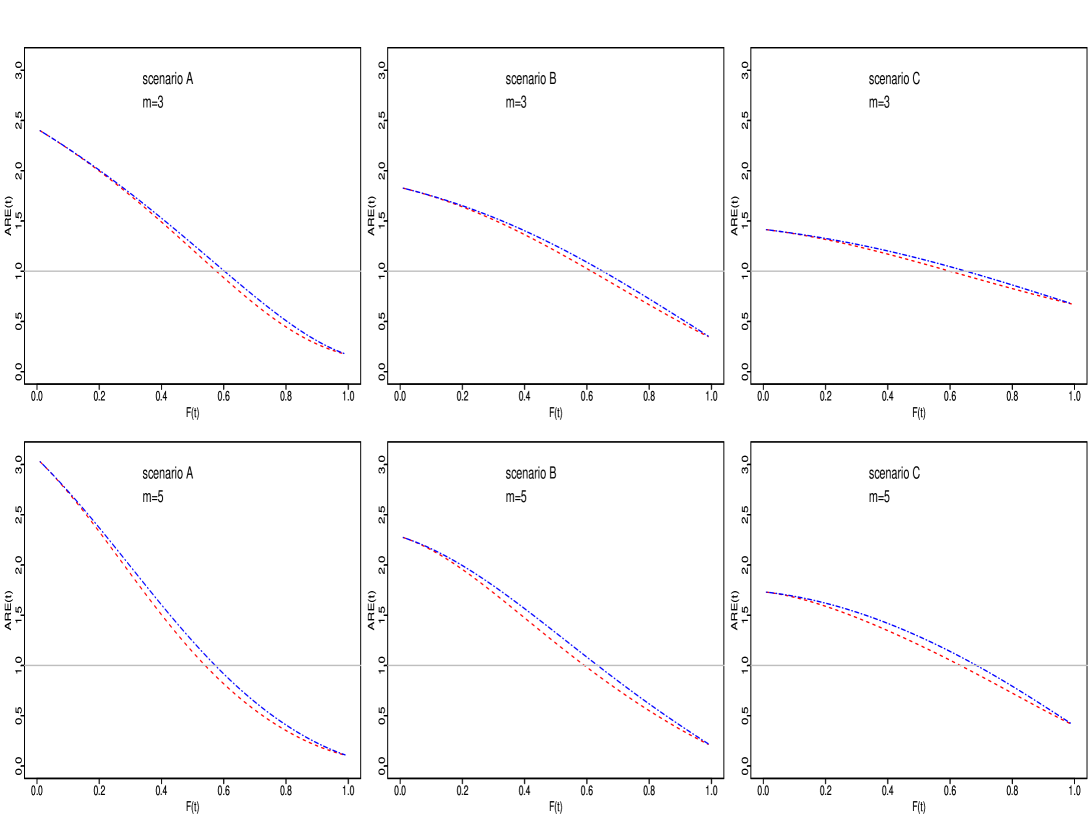
Figure 1: The asymptotic relative efficiency (ARE) of $F_{mb}\left(t\right)$ with respect to $F_{n}\left(t\right)$ is represented by a red dashed line, while that of $F_{ml}\left(t\right)$ with respect to $F_{n}\left(t\right)$ is represented by a blue two-dashed line for $m\in\left\{3,5\right\}$ under three different scenarios for the ties.

Figure 1 shows that the $ARE$s as a function of $F\left(t\right)$ under assumption of perfect ranking. It is worth mentioning that under this assumption, $ARE$s are independent of $F$. It can be observed from Figure 1 that a sizable asymptotic efficiency gain is obtained at the lower tail of the parent distribution as a result of using $F_{mb}\left(t\right)$ or $F_{ml}\left(t\right)$ instead of $F_{n}\left(t\right)$. As it is anticipated, $ARE\left(t\right)$ increases with the set size ($m$) at the lower tail of the parent distribution. However, it decreases when we move from scenario $A$ to scenario $C$. A small asymptotic efficiency gain is observed when $F_{ml}\left(t\right)$ is used instead of $F_{mb}\left(t\right)$ for all values of $t$.

4.2 Finite sample size comparisons

In this sub-section, the finite sample size performances of the CDF estimators are evaluated in the MinPNS and SRS designs using the Monte Carlo simulation. Let $t=Q_{p}$, for $p\in\left[0,1\right],$where $Q_{p}$ is the $p$th quantile of the population distribution. Since $F_{n}\left(t\right)$ is an unbiased estimator for the CDF of the population $\left(F\left(t\right)\right)$, the relative efficiency (RE) of $F_{mb}\left(t\right)$ and $F_{ml}\left(t\right)$ is defined as the ratio of the variance of $F_{n}\left(t\right)$ to the mean square error (MSE) of $F_{mb}\left(t\right)$ and $F_{ml}\left(t\right)$, respectively, i.e.

$$RE\left(p\right)=\frac{\mathbb{V}\left(F_{n}\left(Q_{p}\right)\right)}{MSE\left(F_{z}\left(Q_{p}\right)\right)},$$

for $z=mb$ and $ml.$ With this definition, an $RE\left(p\right)>1$ means that $F_{z}\left(t\right)$ is more efficient than $F_{n}\left(t\right)$ at the point $t=Q_{p}$. By following lines of Proposition 3 in Wang et al. (2012), one can simply show that, under perfect ranking assumption, $RE\left(p\right)$, as a function of $p$, does not depend on the parent distribution.

The Monte Carlo simulation was performed to estimate $RE\left(p\right)$ for both perfect and imperfect ranking cases. The ranking process was done using the linear ranking model introduced by Dell and Clutter (1972). In this model, it is assumed that the variable of interest is $Y$, however, the ranking process is done using the perceived value of $X$. The following relation exists between $X$ and $Y$ :

$$X=\rho\left(\frac{Y-\mu_{y}}{\sigma_{y}}\right)+\sqrt{1-\rho^{2}}Z,$$

where $\mu_{y}$, and $\sigma_{y}$ are the mean and standard deviation of the random variable $Y$, respectively, the random variable $Z$ is independent from $Y$ and follows a standard normal distribution, and parameter $\rho$ is the correlation coefficient between $X$ and $Y$ and controls the quality of ranking. Setting $\rho=1$ gives perfect ranking cases, setting $\rho=0$ gives completely random ranking cases, and choosing $\rho\in\left(0,1\right)$ provides a ranking which is not perfect but is better than random. We set $n\in\left\{30,60,120,600\right\}$, $m\in\left\{3,5\right\}$ and $\rho\in\left\{1,0.75\right\}$. Vector $\mathbf{n}=\left(n_{1},\ldots,n_{m}\right)$ is obtained under three different scenarios similar to those in the Table 2 by multiplying the sample size $n$ by the vector $\mathbf{\lambda}=\left(\lambda_{1},\ldots,\lambda_{m}\right)$, i.e. $\mathbf{n}=\left(\lambda_{1}n,\ldots,\lambda_{m}n\right)$. For each combination of $\left(\mathbf{n},m,\rho\right),$ we drew $100,000$ random samples from the MinPNS and SRS designs when the parent distribution was standard uniform and standard exponential. Finally, $RE\left(p\right)$ was estimated using $100,000$ random samples for $p\in\left\{0.01,\ldots,0.99\right\}$.

Here, only the simulation results for the standard uniform distribution are reported in Figures 2-5. This is because it seems that the type of parent distribution does not have much effect on the pattern of $RE$s in the imperfect ranking case, as well.

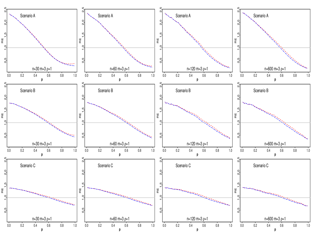
Figure 2: The relative efficiency (RE) of $F_{mb}\left(t\right)$ with respect to $F_{n}\left(t\right)$ represented by a red dashed line and the RE of $F_{ml}\left(t\right)$ with respect to $F_{n}\left(t\right)$ represented by a blue two-dashed line for $n\in\left\{30,60,120,600\right\}$, $m=3$, and $\rho=1$ under three different scenarios for the ties when the parent distribution is standard uniform.

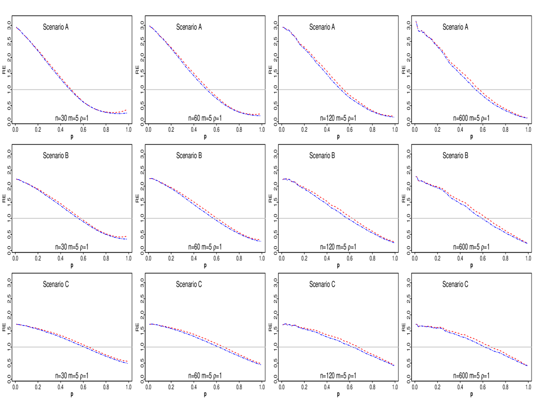
Figure 3: The relative efficiency (RE) of $F_{mb}\left(t\right)$ with respect to $F_{n}\left(t\right)$ represented by a red and $F_{ml}\left(t\right)$ with respect to $F_{n}\left(t\right)$ represented by a blue two-dashed line for $n\in\left\{30,60,120,600\right\}$, $m=5$, and $\rho=1$ under three different scenarios for the ties when the parent distribution is standard uniform.

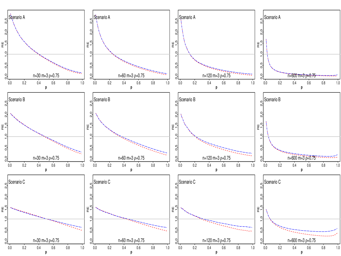
Figure 4: The relative efficiency (RE) of $F_{mb}\left(t\right)$ with respect to $F_{n}\left(t\right)$ represented by a red dashed line and $F_{ml}\left(t\right)$ with respect to $F_{n}\left(t\right)$ represented by a blue two-dashed line for $n\in\left\{30,60,120,600\right\}$, $m=3$, and $\rho=0.75$ under three different scenarios for the ties when the parent distribution is standard uniform.

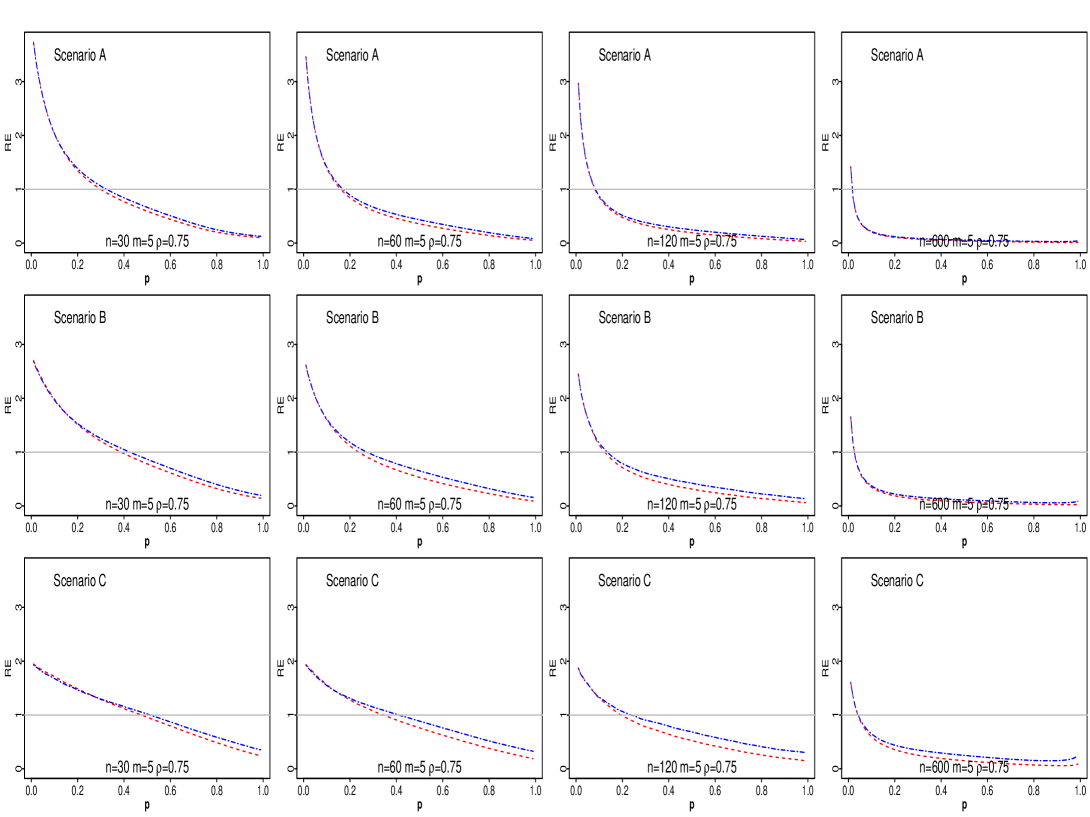
Figure 5: The relative efficiency (RE) of $F_{mb}\left(t\right)$ with respect to $F_{n}\left(t\right)$ represented by a red dashed line and $F_{ml}\left(t\right)$ with respect to $F_{n}\left(t\right)$ represented by a blue two-dashed line for $n\in\left\{30,60,120,600\right\}$, $m=5$, and $\rho=0.75$ under three different scenarios for the ties when the parent distribution is standard uniform.

Figure 2 presents the simulation results for $n\in\left\{30,60,120,600\right\}$, $m=3$, and the perfect ranking case ($\rho=1)$. It can be observed from this figure that the $RE$ patterns of different estimators remain almost the same when the sample size $n$ goes from $n=30$ to $n=600$ However, they decrease when we move from scenario $A$ to scenario $C$ while the other parameters are kept fixed. The highest efficiency gain is attained at the lower tail of the parent distribution under scenario $A$ and the CDF estimators in MinPNS are around $250\%$ more efficient than their counterpart in SRS. As one intuitively expects, the $RE$s fall below one after the median of the parent distribution. This is not a big concern as the MinPNS scheme is designed to deal with situations in which the researcher is interested in drawing a statistical inference for the lower tail of the parent distribution. Similar to what we have observed in Figure 1, although the CDF estimator based on the ML approach is more efficient than the one based on the MB approach, the difference between their $RE$s becomes indistinguishable in some cases, especially at the lower tail of the parent distribution.

The simulation results for $n\in\left\{30,60,120,600\right\}$, $m=5$, and $\rho=1$ are presented in Figure 3. Comparing the results of Figure 2 and Figure 3, it can be observed that the $RE$ patterns for $m=3$ are very similar to those for $m=5$ with the clear difference that the $RE$ pattern are higher for $m=5$ when they are larger than one. In Figure 3 ($m=5$), the highest efficiency gain is obtained at the lower tail of the parent distribution under scenario $A$. The CDF estimators in MinPNS are around $300\%$ more efficient than their counterparts in SRS which is about $50\%$ larger than the case for $m=3$ under scenario $A$ in Figure 2.

The simulation results for the imperfect ranking case ($\rho=0.75$) are depicted in Figures 4 and5 for $m=3$ and $m=5$, respectively. The performance patterns of the estimators in these cases are almost the same as their counterparts in the perfect ranking case ($\rho=1$) with the clear difference that the span of the interval in which the $RE$s are larger than one becomes narrower as we move from $\rho=1$ to $\rho=0.75$.

5 Data Analysis using PNS

Osteoporosis, which literally means porous bone, is a bone disorder in which the density and quality of bone are reduced. As a consequence of this disease, the bone becomes more porous and fragile and thus becomes more likely to break. Bone tissues develop and strengthen from the moment of birth until around the 20s when the bone is at its densest. Bone density remains almost constant for around 10 years later. In their late 30s, people start to lose their bone density slowly as part of the ageing process.

Osteoporosis is a silent disease as it does not have any clear symptoms and develops slowly and progressively. A person may not know that he/she is suffering from it until a minor incidence such as a fall leaves him/her with a fracture. In the absence of a low impact fracture (a fracture occurring spontaneously or from a fall no greater than standing height), osteoporosis is diagnosed based on a low BMD value obtained using DXA technology. Specifically, a person is considered to be suffering from osteoporosis if his/her BMD value obtained using DXA technology is no larger than $0.56$ at either the femoral neck or the lumbar spine.

Osteoporotic fractures impose a huge amount of social and economic burden on the society. For instance, in Europe, the disability rate due to osteoporosis is larger than that caused by cancers (with the exception of lung cancer) and is at least comparable to that caused by different types of chronic diseases such as asthma, rheumatoid arthritis, and high blood pressure-related heart disease (Johnell and Kanis, 2006). Osteoporosis is a common disease and it is estimated that more than 8.9 million osteoporotic fractures happen annually worldwide resulting, on average, in one osteoporotic fracture every 3 seconds (Johnell and Kanis, 2006). Since osteoporosis is an aging-associated disease, it is anticipated that more and more osteoporotic fractures will observed in the future as the global life expectancy has an increasing trend. For instance, it is estimated that by 2035, the annual numbers and costs of osteoporosis-related fractures will be doubled as compared to what was observed in 2010 (Si et al., 2015). Therefore, to minimize the impact of osteoporosis-related fractures on the health of the growing population and the healthcare budget, it is vital for both the government and public health officials to monitor the prevalence of osteoporosis in the society annually.

PNS can be used in the BMD analysis for drawing statistical inference about the lower tail of the underlying distribution as a more cost-efficient technique than SRS. The DXA technology is expensive and not easily accessible in some developing countries. However, a medic can simply rank the patients based on the possibility of suffering from osteoporosis according to his/her personal judgement or an inexpensive covariate. The purpose of this section is to use a real dataset to show the efficiency and applicability of the proposed procedure in a real situation where the ranking procedure is performed using an ordinal concomitant variable so that the ties happen naturally.

5.1 Data description

The World Health Organization (WHO) has recommended using 20-29 year-old non-Hispanic white females from the dataset of the Third National Health and Nutrition Examination Survey (NHANES III) conducted by the National Center for Health Statistics (NCHS) and Centers for Disease Control and Prevention to evaluate the nutritional status and health of a representative sample of the non-institutionalized civilian US population as the reference group for the calculation of the BMD T-score at the femoral neck for both men and women. This national survey which was conducted on 33994 American people from 1988 to 1994 is available online at http://www.cdc.gov/nchs/nhanes/nh3data.htm. The publicty available dataset generated as a result of this survey includes several measurements related to the nutritional status and health of the people included in the survey. Therefore, it can be used to show how PNS can be efficiently used to estimate the prevalence of osteoporosis. Osteoporosis is more common among women than men. Worldwide, 1 in 3 women aged 50 and over will experience at least one osteoporotic fracture, as will 1 in 5 men aged 50 and over (Melton et al., 1992, 1998; Kanis et al., 2000). Due to the importance of the prevalence of osteoporosis among elderly women, we consider the BMD data of the women aged 50 and over in the NHANES III survey as our “hypothetical population” with the size of $N=3978$. We will refer to it hereafter as the ‘BMD dataset’. The summary statistics of the population are reported in Table 3. It is observed that 667 out of 3978 BMD measurements are missing and the average BMD value for the remaining people in the underlying population is $0.799$. Figure 6 shows the histogram of the BMD data superimposed by the normal density function. It is clear from this figure that the normal distribution fits well to the BMD of women aged 50 and over.

$N$	$\#$ NA	$Min$	$Q_{1}$	$Median$	$Q_{3}$	$Max$	$Mean$	$Variance$
3978	667	0.274	0.685	0.793	0.908	1.446	0.799	0.026

Table 3: The summary statistics for the BMD measurements of women aged 50 and over

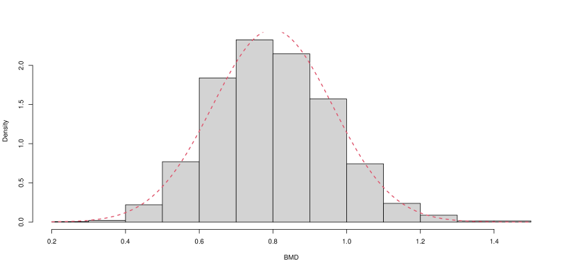
Figure 6: The histogram of the bone mineral density (BMD) measurements of women aged 50 and over along with the fitted normal density curve

Two easily available concomitant variables for ranking are the body mass index category (BMIC) and age decade (AD) variable. The BMIC classifies the participants into four categories according to the recommendation of the WHO as underweight (BMI$<18.5$), normal ($18.5\leq$BMI$<25$), overweight ($25\leq$BMI$<30$), and obese (BMI$\geq 30$). The Spearman correlation coefficient between the BMD and BMIC variables is $0.475$. The ordinal variable AD is obtained from the age of the participants ranging from 50-59, 60-69, …,90+. Moreover, the Spearman correlation coefficient between BMD and AD variables is $-0.466.$ Since the correlation coefficient between BMD and AD is negative, the ranking process is done in reverse. Figure 7 shows the bar charts of the BMIC and AD variables. It is clear from this figure that the frequencies of some levels are higher than those of the others. Hence, when the researcher wants to select the person with highest judgment probability of suffering from osteoporosis using either BMIC or AD variables in a set of small size, ranking ties will easily form.

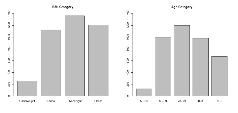
Figure 7: The bar charts of the ranking variables in the BMD dataset: the BMI category and age category

5.2 Empirical study

Let the random variable $Y$ present the actual BMD value of a randomly selected subject from the BMD dataset with the CDF $F$. The prevalence of osteoporosis is this population is given by:

$$F\left(0.56\right)=\mathbb{P}\left(Y\leq 0.56\right)=\int_{0}^{0.56}f\left(y\right)dy=0.061,$$

where $f\left(y\right)$ is the probability density function of the random variable $Y$.

Here, the BMD dataset is used to compare the performances of different CDF estimators in the MinPNS design in estimating the prevalence of osteoporosis by employing the real ties obtained as a result of ranking using the ordinal concomitant variables BMIC and AC. To do so, we set $n\in\left\{10,20,30,40,50,100\right\}$ and $m\in\left\{3,4,5\right\}$. For each combination of $\left(n,m\right)$, we draw $100,000$ random samples from the SRS and MinPNS designs in which all the samplings are done with replacement. To draw a MinPNS sample, we use BMIC (AC) as the ranking variable. In each set with the size of $m,$ a person with the lowest (highest) BMIC (AC) value is selected for actual quantification. If there are two or more people wth the lowest (highest) BMIC (AC) value, one of them is selected at random and the tie information is recorded.

Tables 4 and 5 present the estimated bias, variance, and relative efficiency (RE) of different CDF estimators in MinPNS at point $t=0.56$ for estimating the prevalence of osteoporosis when the ranking variable is BMIC or AC, respectively.

Sample Size	Set size		MB estimator				ML estimator
$n$	$m$		Bias	Variance	RE		Bias	Variance	RE
	3		-0.0101	0.0022	2.4748		-0.0102	0.0022	2.4766
10	4		-0.0140	0.0016	3.0624		-0.0141	0.0016	3.0732
	5		-0.0173	0.0013	3.5142		-0.0174	0.0013	3.5317
	3		-0.0109	0.0010	2.4376		-0.0109	0.0010	2.4395
20	4		-0.0150	0.0007	2.7970		-0.0151	0.0007	2.8027
	5		-0.0182	0.0006	2.9775		-0.0183	0.0006	2.9817
	3		-0.0112	0.0006	2.3220		-0.0112	0.0006	2.3234
30	4		-0.0154	0.0005	2.5323		-0.0154	0.0005	2.5343
	5		-0.0186	0.0004	2.5196		-0.0187	0.0004	2.5198
	3		-0.0112	0.0005	2.2041		-0.0113	0.0005	2.2054
40	4		-0.0157	0.0003	2.2563		-0.0158	0.0003	2.2567
	5		-0.0187	0.0003	2.1816		-0.0188	0.0003	2.1785
	3		-0.0113	0.0004	2.0982		-0.0114	0.0004	2.0995
50	4		-0.0156	0.0003	2.0800		-0.0157	0.0003	2.0787
	5		-0.0187	0.0002	1.9210		-0.0188	0.0002	1.9158
	3		-0.0117	0.0002	1.6809		-0.0117	0.0002	1.6801
100	4		-0.0157	0.0001	1.4268		-0.0158	0.0001	1.4228
	5		-0.0190	0.0001	1.1868		-0.0191	0.0001	1.1807

Table 4: The empirical study using the BMD dataset: comparing the performances of different estimators in estimating the prevalence of osteoporosis when ranking is done using the BMI category ($\rho=0.478$)

Sample Size	Set size		MB estimator				ML estimator
$n$	$m$		Bias	Variance	RE		Bias	Variance	RE
	3		-0.0096	0.0021	2.5487		-0.0096	0.0021	2.5488
10	4		-0.0135	0.0016	3.1815		-0.0136	0.0016	3.1926
	5		-0.0169	0.0012	3.6779		-0.0171	0.0012	3.6921
	3		-0.0107	0.0010	2.5056		-0.0107	0.0010	2.5062
20	4		-0.0148	0.0007	2.9318		-0.0148	0.0007	2.9368
	5		-0.0180	0.0005	3.1002		-0.0181	0.0005	3.1042
	3		-0.0108	0.0006	2.4007		-0.0108	0.0006	2.4010
30	4		-0.0149	0.0004	2.6463		-0.0150	0.0004	2.6478
	5		-0.0182	0.0003	2.6324		-0.0183	0.0003	2.6321
	3		-0.0109	0.0005	2.2797		-0.0109	0.0005	2.2802
40	4		-0.0152	0.0003	2.3682		-0.0152	0.0003	2.3683
	5		-0.0186	0.0002	2.2443		-0.0187	0.0002	2.2403
	3		-0.0110	0.0004	2.1884		-0.0110	0.0004	2.1892
50	4		-0.0153	0.0002	2.1522		-0.0154	0.0002	2.1507
	5		-0.0186	0.0002	1.9824		-0.0187	0.0002	1.9766
	3		-0.0114	0.0002	1.7353		-0.0114	0.0002	1.7351
100	4		-0.0155	0.0001	1.4815		-0.0155	0.0001	1.4776
	5		-0.0187	0.0001	1.2279		-0.0188	0.0001	1.2213

Table 5: The empirical study using the BMD dataset: comparing the performances of different estimators in estimating the prevalence of osteoporosis when ranking is done using age category ($\rho=0.469$)

Table 4 presents the results when the ranking is done using the BMIC. It can be observed from this table that the efficiency gain using PNS estimators can be as large as $350\%$ in some certain circumstances and never falls below one. For $n\leq 30$, the REs of both ML and MB estimators are increasing functions in $m$. For $n=40,$ the REs increase when we move from $m=3$ to $m=4$ and decrease when we move from $m=4$ to $m=5$. For $n\geq 50$, the REs are decreasing functions in $m$. It should be noted that both estimators slightly underestimate the true value of the prevalence of osteoporosis. It is worth mentioning that both ML and MB estimators have competitive performance in all the considered cases which is consistent with what was observed in Section 4.

Table 5 presents the results when AC is used as the ranking variable. Although the REs are slightly higher in this table, their patterns are very similar to those in Table 4.

5.3 Revisiting an earlier example

Assume that the sample units in Table 1 are obtained from the BMD dataset and we want to compare the estimators using the example given in Section 2. Based on the data and the tie information in Table 1, we produce $F_{ml}\left(0.56\right)=0.0357$ and $F_{mb}\left(0.56\right)=0.0352$. It can be observed that the ML estimator produces a slightly closer value to the true value of the parameter of interest $\left(F\left(0.56\right)=0.061\right)$.

6 Concluding remarks

In this paper, a new cost-efficient sampling scheme was developed for drawing statistical inference about either the lower or the upper tail of the population distribution. The proposed procedure can be applied in the situations in which measuring the variable of interest is time-consuming, costly, and/or destructive. However, a small number of the sampling units (set) can be ranked without taking the actual measurements on them. In principle, the proposed procedure is similar to nomination sampling (NS) with a clear modification which is made to increase the applicability of this design in practice. In fact, NS cannot be performed unless the researcher is able to determine with a high confidence the sample unit with the lowest/highest rank in the set . We proposed to modify NS in a way that the researcher is allowed to declare as many ties as needed whenever he/she cannot find with a high confidence the sample unit with the lowest/highest rank in the set . In partial nomination sampling (PNS), the researcher divides the sample units in the set into two subsets in a way that the sample units in the first subset are all smaller than those in the second one. However, the subset units in the second subset need not be ranked. Finally, the researcher selects one unit at random from the first (second) subset to obtain the Min(Max)PNS.

Then, two the cumulative distribution function (CDF) estimators were developed based on the maximum likelihood (ML) and moment-based (MB) approaches and the asymptotic normality of each of them was proved. It was shown that under the perfect ranking assumption, the ML estimator of the CDF was asymptotically more efficient than the MB estimator, although the efficiency gain was rather small. For various choices of sample size, set size, parent distribution, ties generation mechanism, and quality of ranking, we compared the proposed estimators in PNS with their counterparts in SRS using the Monte Carlo simulation. The simulation results indicated that the developed estimators had very competitive performances and were significantly more efficient than their counterparts in simple random sampling (SRS) at either the lower or the upper tail of the population distribution.

Finally, the proposed procedure was applied to a BMD dataset from the Third National Health and Nutrition Examination Survey (NHANES III) to estimate the prevalence of osteoporosis in adult women aged 50 and over. The ranking was done using the two inexpensive and easily available ranking variables of body mass index and age category where the ties naturally happened in the ranking process. It was observed that MinPNS substantially improved the efficiency of the estimation of osteoporosis. Therefore, it considerably reduced the time and cost of the study. The findings of this paper encourage using the PNS design to incorporate partial rank information into the estimation process.

This work was the first but important attempt in developing statistical inference about either the lower or the upper tail of the population distribution using PNS. Therefore, it remains an ample space for future research. For instance, the proposed methodology in this paper can be used for estimating other population attributes rather than the CDF. Let $\theta=g\left(F\right)$ be the parameter of interest where $g\left(.\right)$ is an arbitrary function. This parameter can be estimated in PNS by replacing the CDF of $F$ with the proposed estimators in PNS. With the efficiency gain of the CDF estimators in PNS, it is intuitively expected that the resulting estimators of $\theta$ will perform well in some certain circumstances. Moreover, note that the asymptotic normality of the proposed methodology in this paper requires the perfect ranking assumption which may not hold in some practical situations. This, combined with the fact that a large enough sample size is needed to use the normal theory of the estimators which may not be available in cost-efficient sampling designs such as PNS, reminds us that using some alternative methods (such as bootstrap techniques) is vital. These topics can be addressed in subsequent works.

Data availability statement

The data that support the findings of this study are obtained from the third National Health and Nutrition Examination Survey (NHANES III) and is available online at

http://www.cdc.gov/nchs/nhanes/nh3data.htm.

References

- Al-Omari and Haq (2011) Al-Omari, A. I., and Haq, A., 2011, Improved quality control charts for monitoring the process mean, using double-ranked set sampling methods. Journal of Applied Statistics, 39 (4), 745-763.
- Ahn et al. (2017) Ahn, S., Wang, X., and Lim, J. 2017. On unbalanced group sizes in cluster randomized designs using balanced ranked set sampling, Statistics and Probability Letters, 123, 210-217.
- Chen et al. (2005) Chen, H., Stasny, E. A., Wolfe, D.A., 2005. Ranked set sampling for efficient estimation of a population proportion. Statistics in Medicine 24, 3319-3329.
- Chen et al. (2018) Chen, W., Tian, Y., Xie, M. 2018. The global minimum variance unbiased estimator of the parameter for a truncated parameter family under the optimal ranked set sampling, Journal of Statistical Computation and Simulation, 8 (17), 3399-3414
- Chen et al. (2019) Chen, W., Yang, R., Yao, D., Long, C. 2019. Pareto parameters estimation using moving extremes ranked set sampling, To appear in Statistical Papers.
- Boyles and Samaniego (1986) Boyles, R. A., and Samaniego, F. J. 1986. Estimating a distribution function based on nomination sampling, Journal of the American Statistical Association, 81 (396), 1039-1045.
- Dell and Clutter (1972) Dell, T.R., and Clutter, J.L., 1972. Ranked set sampling theory with order statistics background. Biometrics 28, 2, 545-555.
- Duembgen and Zamanzade (2020) Duembgen, L., and Zamanzade, 2020. Inference on a distribution function from ranked set samples. Annals of the institute of Statistical Mathematics, 72, 157–185.
- Frey (2012) Frey, J. 2012. Nonparametric mean estimation using partially ordered sets. Environmental and Ecological Statistics, 19 (3), 309-326.
- Frey and Wang (2013) Frey, J., and Wang, L. 2013. Most powerful rank tests for perfect rankings, Computational Statistics and Data Analysis, 60, 157-168.
- Frey and Wang (2014) Frey, J., and Wang, L. 2014. EDF-based goodness-of-fit tests for ranked-set sampling, Canadian Journal of Statistics, 42 (3), 451-469.
- Frey and Feeman (2016) Frey, J., and Feeman, T.G. 2016. Efficiency comparisons for partially rank-ordered set sampling. Statistical Papers, 58 (4), 1149-1166.
- Frey and Zhang (2017) Frey, J., and Zhang, Y. 2017. Testing perfect rankings in ranked-set sampling with binary data. Canadian Journal of Statistics, 45 (3), 326-339.
- Frey et al. (2007) Frey, J., Ozturk , O., and Deshpande, J. V. 2007. Nonparametric tests for perfect judgment ranking, Journal of the American Statistical Association, 102 (478), 708-717.
- Frey and Zhang (2019) Frey, J. and Zhang, Y. 2019. Improved exact confidence intervals for a proportion using ranked set sampling, Journal of the Korean Statistical Society, 48 (3), 493-501.
- Frey and Zhang (2021) Frey, J. and Zhang, Y. 2021. Robust confidence intervals for a proportion using ranked-set sampling, To appear in Journal of the Korean Statistical Society .
- He et al. (2020) He, X., Chen, W., and Qian, W. 2020. Maximum likelihood estimators of the parameters of the log-logistic distribution, Statistical Papers, 61, 1875-1892.
- He et al. (2021) He, X., Chen, W., and Rui, Y. 2021. Modified best linear unbiased estimator of the shape parameter of log-logistic distribution, Journal of Statistical Computation and Simulation, 91 (2), 383-395.
- Hjort and Pollard (2011) Hjort, N.L., and Pollard, D. 2011. Asymptotics for minimisers of convex processes. arXiv:1107.3806v1 [math.ST]
- Johnell and Kanis (2006) Johnell, O., and Kanis, J. A. 2006. An estimate of the worldwide prevalence and disability associated with osteoporotic fractures. Osteoporos Int 17:1726.
- Jafari Jozani and Mirkamali (2010) Jafari Jozani, M. and Mirkamali, S. J. 2010. Improved attribute acceptance sampling plans based on maxima nomination sampling. Journal of Statistical Planning and Inference. 140, 2448-2460.
- Jafari Jozani and Mirkamali (2011) Jafari Jozani M, Mirkamali S. J. 2011. Control charts for attributes with maxima nominated samples. Journal of Statistical Planning and Inference;141:2386-2398.
- Jafari Jozani et al. (2018) Jafari Jozani, M., Ayilara, O. F., and Leslie, W. B. 2018. Quantile regression with nominated samples: An application to a bone mineral density study . Statistics in Medicine, 37 (14), 2267-2283.
- Haq et al. (2013) Haq, A., Brown, J., Moltchanova, E., and Al-Omari, A. I. 2013. Partial ranked set sampling design, Environmetrics, 24 (3), 201-207.
- Haq and Al-Omari (2014) Haq, A., and Al-Omari, A. I., 2014, A new Shewhart control chart for monitoring process mean based on partially ordered judgment subset sampling, Quality and Quantity, 49 (3), 1185-1202.
- Haq et al. (2014) Haq, A., Brown, J., Moltchanova, E., and Al-Omari, A. 2014. Effect of measurement error on exponentially weighted moving average control charts under ranked set sampling schemes, Journal of Statistical Computation and Simulation, 85 (6), 1224-1246.
- Kanis et al. (2000) Kanis J A, Johnell O, Oden A, et al. 2000. Long-term risk of osteoporotic fracture in Malmo. Osteoporos Int 11:669.
- Melton et al. (1998) Melton L J, Atkinson E J, O’Connor MK, et al. 1998. Bone density and fracture risk in men. J Bone Miner Res 13:1915.
- Melton et al. (1992) Melton L J, Chrischilles E A, Cooper C, et al. 1992. Perspective. How many women have osteoporosis? J Bone Miner Res 7:1005.
- McIntyre (1952) McIntyre, G.A., 1952. A method for unbiased selective sampling using ranked set sampling. Austral. J. Agricultural Res. 3, 385-390.
- Mu (2015) Mu, X., 2015. Log-concavity of a mixture of beta distributions, Statistics and Probability Letters, 99, 125-130
- Nourmohammadi et al. (2014) Nourmohammadi, M., Jafari Jozani, M. and Johnson, B. 2014. Confidence interval for quantiles in finite populations with randomized nomination sampling. Computational Statistics and Data Analysis. 73, 112–128.
- Omidvar et al. (2018) Omidvar, S., Jafari Jozani, M. and Nematollahi, N. 2018. Judgment post-stratification in finite mixture modeling: An example in estimating the prevalence of osteoporosis, Statistics in Medicine, 37 (30), 4823-4836
- Ozturk (2011) Ozturk, O. 2011. Sampling from partially rank-ordered sets. Environmental and Ecological Statistics, 18, 757-779.
- Qian et al. (2021) Qian, W., Chen, W., He, X. 2021. Parameter estimation for the Pareto distribution based on ranked set sampling. Statistical Papers, 62, 395-417.
- Samawi and Al-Sagheer (2001) Samawi, H. M., and Al-Sagheer, O. A. 2001. On the estimation of the distribution function using extreme and median ranked set samples. Biometrical Journal, 43 (3), 357-373.
- Samawi and Al-Saleh (2013) Samawi, H. M., and Al-Saleh, M.F. 2013. Valid estimation of odds ratio using two types of moving extreme ranked set sampling. Journal of the Korean Statistical Society 42, 17-24.
- Samawi et al. (2017) Samawi, H. M., Rochani, H., Linder, D., and Chatterjee, A. 2017. More efficient logistic analysis using moving extreme ranked set sampling. Journal of Applied Statistics, 44 (4), 753-76.
- Samawi et al. (2017) Samawi, H. M., Yin, J., Rochani, H., Panchal, V. 2017. Notes on the overlap measure as an alternative to the Youden index: How are they related? Statistics in Medicine, 36 (26), 4230-4240.
- Samawi et al. (2018) Samawi, H. M., Helu, A., Rochani, H., Yin, J., Yu, L., and Vogel, R. 2018. Reducing sample size needed for accelerated failure time model using more efficient sampling methods. Statistical Theory and Practice, 12 (3), 530-541.
- Si et al. (2015) Si, L., Winzenberg, T. M., Jiang, Q., Chen, M., Palmer, A. J. 2015.Projection of osteoporosis-related fractures and costs in China: 2010–2050. Osteoporos Int 26, 1929-1937.
- Stokes and Sager (1988) Stokes, S. L., and Sager, T. W. Characterization of a ranked-set sample with application to estimating distribution functions. Journal of the American Statistical Association, 83 (402), 374-381.
- Takahasi and Wakitomo (1968) Takahasi, K., and Wakimoto, K. 1968. On unbiased estimates of the population mean based on the sample stratified by means of ordering. Annals of the Institute of Statistical Mathematics, 20(1), 1-31
- Wang et al. (2012) Wang, X., Wang, K., and Lim, J. 2012. Isotonized CDF estimation from judgment poststratification data with empty strata. Biometrics, 61 (1), 194-202.
- Wang et al. (2016) Wang, X., Lim, J., and Stokes, S. L. 2016. Using ranked set sampling with cluster randomized designs for improved inference on treatment effects. Journal of the American Statistical Association, 111 (516), 1576-1590.
- Wang et al. (2017) Wang, X., Ahn, S., and Lim, J. 2017. Unbalanced ranked set sampling in cluster randomized studies. Journal of Statistical Planning and Inference, 187, 1-16.
- Wang et al. (2020) Wang, X., Wang, M., Lim, J., and Ahn, S. 2020. Using ranked set sampling with binary outcomes in cluster randomized designs. Canadian Journal of Statistics, 48 (3), 342-365.
- Willemain (1980) Willemain, T. 1980a. A comparison of patient-centered and case-mix reimbursement for nursing home care, Health Service Research, 15 (4), 365-377.
- Willemain (1980) Willemain T. 1980. Estimating the population median by nomination sampling. Journal of American Statistical Association.75 (372):908-911.
- Zamanzade and Mahdizadeh (2017) Zamanzade, E. and Mahdizadeh, M. 2017. A more efficient proportion estimator in ranked set sampling. Statistics and Probability Letters, 129, 28-33.
- Zamanzade and Mahdizadeh (2020) Zamanzade, E., and Mahdizadeh, M. 2020. Using ranked set sampling with extreme ranks in estimating the population proportion, Statistical Methods in Medical Research, 29 (1), 165-177.