Reducing the Deployment-Time Inference Control Costs of
Deep Reinforcement Learning Agents via an Asymmetric Architecture

Abstract

Deep reinforcement learning (DRL) has been demonstrated to provide promising results in several challenging decision making and control tasks. However, the required inference costs of deep neural networks (DNNs) could prevent DRL from being applied to mobile robots which cannot afford high energy-consuming computations. To enable DRL methods to be affordable in such energy-limited platforms, we propose an asymmetric architecture that reduces the overall inference costs via switching between a computationally expensive policy and an economic one. The experimental results evaluated on a number of representative benchmark suites for robotic control tasks demonstrate that our method is able to reduce the inference costs while retaining the agent’s overall performance.

I Introduction

Recent works have combined reinforcement learning (RL) with the advances of deep neural networks (DNNs) to make breakthroughs in domains ranging from games [1, 2, 3] to robotic control [4, 5, 6]. However, the inference phase of a DNN model is a computationally-intensive process [7, 8] and is one of the major concerns when applied to mobile robots, which are mostly battery-powered and have limitations on the energy budgets. Although the energy consumption of DNNs could be alleviated by reducing their sizes for energy-limited platforms, smaller DNNs are usually not able to attain same or comparable levels of performances as larger ones in complex scenarios. On the other hand, the performances of smaller DNNs may still be acceptable in some cases. For example, a small DNN unable to perform complex steering control is still sufficient to handle simple and straight roads. Motivated by this observation, we propose an asymmetric architecture that selects a small DNN to act when conditions are acceptable, while employing a large one when necessary.

We implement this cost-efficient asymmetric architecture via leveraging the concept from hierarchical reinforcement learning (HRL) [9], which consists of a master policy and two sub-policies. The master policy is designed as a lightweight DNN for decision-making, which takes in a state as its input and learns to choose a sub-policy based on the input state. The two sub-policies are separately implemented as a large DNN and a small DNN. The former is designed to deal with complicated state-action mapping, while the latter is responsible for handling simple scenarios. Therefore, when complex action control is required, the master policy uses the former. Otherwise, the latter is selected. To achieve the objective of cost-aware control, we propose a loss function design such that the inference costs of executing the two sub-policies are taken into consideration by the master policy. The master policy is required to learn to use the sub-policy with a small DNN as frequently as possible while maximizing and maintaining the agent’s overall performance.

Our principal contribution is an asymmetric RL architecture that reduces the deployment-time inference costs. To validate the proposed architecture, we perform a set of experiments on the representative robotic control tasks from the OpenAI Gym Benchmark Suite [10] and the DeepMind Control Suite [11]. The results show that the master policy trained by our methodology is able to alternate between the two sub-policies to save inference costs in terms of floating-point operations (FLOPs) with little performance drop. We further provide an in-depth look into the behaviors of the trained master policies, and quantitatively and qualitatively discuss why the computational costs can be reduced. Finally, we offer a set of ablation analyses to validate the design decisions of our cost-aware methodology.

II Related Work

A number of knowledge distillation based methods have been proposed in the literature to reduce the inference costs of DRL agents at the deployment time [12, 13, 14, 15]. These methods typically use a large teacher network to teach a small student network such that the latter is able to mimic the behaviors of the former. In contrast, our asymmetric approach is based on the concept of HRL [9], a framework consisting of a policy over sub-policies and a number of sub-policies for executing temporally extended actions to solve sub-tasks. Previous HRL works [16, 17, 18, 19, 20, 21, 22, 23, 24] have been concentrating on using temporal abstraction to deal with difficult long-horizon problems. As opposed to those prior works, our proposed method focuses on employing HRL to reduce the inference costs of an RL agent. Please note that the theme and objective of the paper is to propose a new direction of HRL to a practical problem in robot deployment scenarios, not a more general HRL strategy.

III Background

III-A Reinforcement Learning

We consider the standard RL setup where an agent interacts with an environment $\mathcal{E}$ over a number of discrete timesteps, where the interaction is modeled as a Markov Decision Process (MDP). At each timestep $t$, the agent observes a state $s_{t}$ from a state space $\mathcal{S}$, and performs an action $a_{t}$ from an action space $\mathcal{A}$ according to its policy $\pi$, where $\pi$ is a mapping function represented as $\pi:\mathcal{S}\to P(\mathcal{A})$. The agent then receives the next state $s_{t+1}\in\mathcal{S}$ and a reward signal $r_{t}$ from $\mathcal{E}$. The process continues until a termination condition is met. The objective of the agent is to maximize the expected cumulative return $\mathbb{E}[R_{t}]=\mathbb{E}[\Sigma_{k=0}^{\infty}\gamma^{k}r_{t+k}]$ from $\mathcal{E}$ for each timestep $t$, where $\gamma\in(0,1]$ is a discount factor.

III-B Hierarchical Reinforcement Learning

HRL introduces the concept of ‘options’ into the RL framework, where options are temporally extended actions. [9] shows that an MDP combined with options becomes a Semi-Markov Decision Process (SMDP). Assume that there exists a set of options $\Omega$. HRL allows a ‘policy over options’ $\pi_{\Omega}$ to determine an option for execution for a certain amount of time. Each option $\omega\in\Omega$ consists of three components $(\mathcal{I}_{\omega},\pi_{\omega},\mathcal{\beta}_{\omega})$, in which $\mathcal{I}_{\omega}\subseteq\mathcal{S}$ is an initial set according to $\pi_{\Omega}$, $\pi_{\omega}$ is a policy following option $\omega$, and $\mathcal{\beta}_{\omega}:\mathcal{S}\to[0,1]$ is a termination function. When an agent enters a state $s\in\mathcal{I}_{\omega}$, option $\omega$ is adopted, and policy $\pi_{\omega}$ is followed until a state $s_{k}$ where $\beta_{\omega}(s_{k})\to 1$. In episodic tasks, termination of an episode also terminates the current option. Our architecture is a special case of SMDP. Section IV introduces our update rules for $\pi_{\Omega}$ and $\pi_{\omega}$. In this paper, we refer to a ‘policy over options’ as a master policy, and an ‘option’ as a sub-policy.

IV Methodology

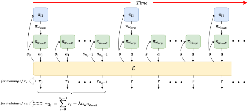
Figure 1: An illustration of the workflow of our framework. The master policy $\pi_{\Omega}$ chooses a sub-policy $\pi_{\omega}\in\{\pi_{\omega_{small}},\pi_{\omega_{large}}\}$, and uses it to interact with the environment $\mathcal{E}$ for $n_{\omega}$ timesteps. After this, $\pi_{\Omega}$ chooses another $\pi_{\omega}$, and the process repeats until the end of the episode. $\pi_{\Omega}$ and $\pi_{\omega}$ use different experience transitions to update their policies and have different replay buffers, while $\pi_{\omega_{small}}$ and $\pi_{\omega_{large}}$ share the same replay buffer. We train $\pi_{\omega_{small}}$ and $\pi_{\omega_{large}}$ with experience transitions $(s_{t},a_{t},r_{t},s_{t+1})\text{ for }t=0,1,...,etc$, and train $\pi_{\Omega}$ with transitions $(s_{t},\omega_{t},r_{\Omega_{t}},s_{t+n_{\omega}})\text{ for }t=0$, $\,n_{\omega},...,etc$. The reward $r_{\Omega_{t}}=\Sigma_{i=t}^{t+n_{\omega}-1}r_{i}\allowbreak-\lambda n_{\omega}c_{\omega_{t}}$ of $\pi_{\Omega}$ is the sum of rewards $r_{i}$ collected by $\pi_{\omega}$, which is penalized by the scaled cost $\lambda n_{\omega}c_{\omega_{t}}$ of $\pi_{\omega}$. Note that $\lambda$ is a scaling parameter.

IV-A Problem Formulation

The main objective of this research is to develop a cost-aware strategy such that an agent trained by our methodology is able to deliver satisfying performance while reducing its overall inference costs. We formulate the problem as an SMDP, with an aim to train the master policy in the proposed framework to use the smaller sub-policy when the condition is appropriate to be handled by it, and employ the larger sub-policy when the agent requires complex control of its actions. The agent is expected to use the smaller sub-policy as often as possible to reduce its computational costs. In order to incorporate the consideration of inference costs into our cost-aware strategy, we further assume that each sub-policy is cost-bounded. The cost of a sub-policy is denoted as $c_{\omega}$, where $\omega$ represents the sub-policy used by the agent. The reward function is designed such that the agent is encouraged to select the lightweight sub-policy as frequently as possible to avoid being penalized.

IV-B Overview of the Cost-Aware Framework

In order to address the problem formulated above, we employ an HRL framework consisting of a master policy $\pi_{\Omega}$ and two sub-policies $\pi_{\omega}$ of different DNN sizes, where $\omega\in\{\omega_{small},\omega_{large}\}$ and the DNN size of $\omega_{large}$ is larger than that of $\omega_{small}$. We assume that both the sub-policies $\pi_{\omega}$ can be completed in a single timestep. At the beginning of a task, $\pi_{\Omega}$ first takes in the current state $s\in\mathcal{S}$ from $\mathcal{E}$ to determine which $\pi_{\omega}$ to use. The selected $\pi_{\omega}$ is then used to interact with $\mathcal{E}$ for $n_{\omega}$ timesteps, i.e., $\mathcal{\beta}_{\omega}\to 1$ once the selected sub-policy $\omega$ is used for $n_{\omega}$ timesteps. The value of $n_{\omega}$ is set to be a constant for the two sub-policies, i.e., $n_{\omega_{large}}=n_{\omega_{small}}$. The process repeats until the end of the episode. The workflow of the proposed cost-aware hierarchical framework is illustrated in Fig. 1. Please note that even though the overall system is formulated as an SMDP, the formulation for $\pi_{\Omega}$ is still a standard MDP problem of selecting between a set of two temporally extended actions (i.e., using either $\pi_{\omega_{small}}$ or $\pi_{\omega_{large}}$), as described in Section 3 of [9]. Therefore, at timestep $t$, the goal of $\pi_{\Omega}$ becomes maximizing $R_{\Omega_{t}}=\Sigma_{i=0}^{\infty}\gamma^{i}r_{\Omega_{t+i\cdot n_{\omega}}}$, where $r_{\Omega_{t}}=\Sigma_{j=t}^{t+n_{\omega}-1}r_{j}$ is the cumulative rewards during the execution of $\pi_{\omega}$. On the other hand, the update rule of $\pi_{\omega}$ is the same as the intra-option policy gradient described in [17]. To deal with the data imbalance issue of the two sub-policies during the training phase as well as improving data efficiency, our cost-aware framework uses an off-policy RL algorithm for $\pi_{\omega}$ so as to allow $\pi_{\omega_{small}}$ and $\pi_{\omega_{large}}$ to share the common experience replay buffer.

IV-C Cost-Aware Training

We next describe the training methodology. In case that no regularization is applied, $\pi_{\Omega}$ tends to choose $\pi_{\omega_{large}}$ due to its inherent advantages of being able to obtain more rewards on its own. As a result, we penalize $\pi_{\Omega}$ with $c_{\omega}$ to encourage it to choose $\pi_{\omega_{small}}$ with a lower $c_{\omega}$. The reward for $\pi_{\Omega}$ at $t$ is thus modified to $r_{t}-\lambda c_{\omega}$, where $\lambda$ is a cost coefficient for scaling. The higher the value of $\lambda$ is, the more likely $\pi_{\Omega}$ will choose $\pi_{\omega_{small}}$. The experience transitions used to update $\pi_{\Omega}$ are therefore expressed as $(s_{t},\omega_{t},r_{\Omega_{t}},s_{t+n_{\omega}})\text{ for }t=0$, $n_{\omega},2n_{\omega},...,etc$, where $r_{\Omega_{t}}=\Sigma_{i=t}^{t+n_{\omega}-1}r_{i}-\lambda n_{\omega}c_{\omega_{t}}$.

V Experimental Results

V-A Experimental Setup

V-A1 Environments

We verify the proposed methodology in simple classic control tasks from the OpenAI Gym Benchmark Suite [10], and a number of challenging continuous control tasks from both the OpenAI Gym Benchmark Suite and the DeepMind Control Suite [11] simulated by the MuJoCo [25] physics engine. The challenging tasks include four continuous control tasks from the OpenAI Gym Benchmark Suite, and two tasks from the DeepMind Control Suite.

V-A2 Hyperparameters

TABLE I: The detailed settings of the hyperparameters adopted by the master policy $\pi_{\Omega}$ and the sub-policies $\pi_{\omega}$ of our methodology.

Hyperparameter	Value	Hyperparameter	Value
Master Policy $\pi_{\Omega}$		Sub-Policy $\pi_{\omega}$
RL algorithm	DQN	RL algorithm	SAC
Learning rate	$1\mathrm{e}{-3}$	Entropy coefficient $\alpha$	Auto
Discount factor ($\gamma$)	$0.99$	Learning rate of agent	$3\mathrm{e}{-4}$
Replay buffer size	50K	Discount factor ($\gamma$)	$0.99$
Exploration fraction	10%	Replay buffer size	1M
Update batch size	32	Update batch size	256
Double Q	True	Train frequency	1
Train frequency	1	Target soft update coefficient $\tau$	0.005
Target network update interval	500	Target network update interval	1
Optimization for the RL agent	Adam	Optimization for the RL agent	Adam
Training timesteps	2.5M	Training timesteps	2.5M
Nonlinearity	Tanh	Nonlinearity	Tanh

TABLE II: Number of neurons $n_{units}$ per layer for $\pi_{\omega_{small}}$ & $\pi_{\omega_{large}}$, $c_{\omega_{small}}$, $c_{\omega_{large}}$, and $\lambda$ for each robotic control tasks.

Environment	$n_{units}$ for $\pi_{\omega_{small}}$	$n_{units}$ for $\pi_{\omega_{large}}$	$c_{\omega_{small}}$	$c_{\omega_{large}}$	$\lambda$
MountainCarContinuous-v0	$8$	$64$	$1.0$	$44.7$	$1\mathrm{e}{-4}$
Swimmer-v3	$8$	$256$	$1.0$	$428.4$	$1\mathrm{e}{-4}$
Ant-v3	$64$	$256$	$1.0$	$8.0$	$1\mathrm{e}{-1}$
FetchPickAndPlace-v1	$32$	$128$	$1.0$	$9.4$	$2\mathrm{e}{-4}$
walker-stand	$8$	$64$	$1.0$	$18.1$	$1\mathrm{e}{-2}$
finger-spin	$8$	$64$	$1.0$	$29.1$	$1\mathrm{e}{-2}$

In our experiments, the master policy $\pi_{\Omega}$ is implemented as a Deep Q-Network (DQN) [1] agent to discretely choose between the two sub-policies. On the other hand, the sub-policies $\pi_{\omega}$ are implemented as Soft Actor-Critic (SAC) [5] agents for performing the continuous control tasks described above. The hyperparameters used for training are shown in Table I. Both $\pi_{\Omega}$ and $\pi_{\omega}$ are implemented as multilayer perceptrons (MLPs) with two hidden layers. We set the number of units $n_{units}$ per layer for $\pi_{\Omega}$ to 32 for all tasks, and determine $n_{units}$ for $\pi_{\omega}$ as follows. We first train a model with $n_{units}$ set to 512 as the criterion model, and then find the minimum $n_{units}$ for the model which can achieve $90\%$ of the performance of the criterion model. We use this as $n_{units}$ for $\pi_{\omega_{large}}$. And then we find $n_{units}$ for $\pi_{\omega_{small}}$, such that its value is less than or equal to $1/4$ of $n_{units}$ for $\pi_{\omega_{large}}$ and the performance of $\pi_{\omega_{small}}$ is around or below $1/3$ of the score achieved by the criterion model.

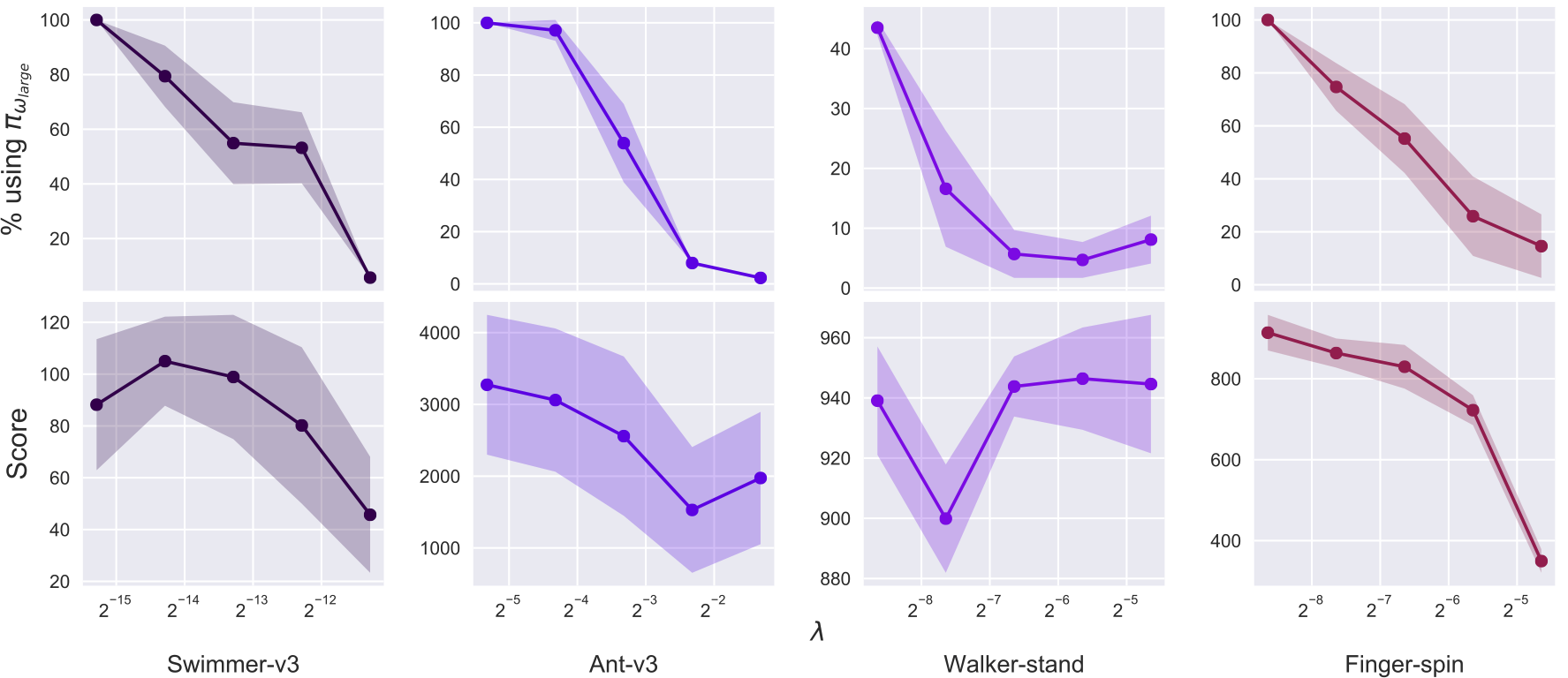
Figure 2: Performance of the models trained with different $\lambda$. The scores are averaged from 5 different random seeds. Each model trained with different random seed is evaluated over 200 episodes.

For the cost term, we adopt the inference FLOPs of $\pi_{\omega}$ as $c_{\omega}$, since the FLOPs executed by $\pi_{\omega}$ and its energy consumption are correlated. We use the number of FLOPs of $\pi_{\omega_{small}}$ and $\pi_{\omega_{large}}$ divided by the number of FLOPs of $\pi_{\omega_{small}}$ as their policy costs $c_{\omega_{small}}$ and $c_{\omega_{large}}$, respectively, such that $c_{\omega_{small}}$ is equal to one. With regard to $\lambda$, from Fig. 2, we observe that $\lambda$ and the ratio of choosing $\pi_{\omega_{large}}$ is negatively correlated. Even though the performances decline along with the reduced usage rate of $\pi_{\omega_{large}}$, there is often a range of $\lambda$ which leads to lower usage rate of $\pi_{\omega_{large}}$ and yet comparable performance to the model of high $\pi_{\omega_{large}}$ usage rate. We perform a hyperparameter search to find an appropriate $\lambda$, such that both $\pi_{\omega_{small}}$ and $\pi_{\omega_{large}}$ are used alternately within an episode, while allowing the agent to obtain high scores. The hyperparameters used in the cost term are listed in Table II.

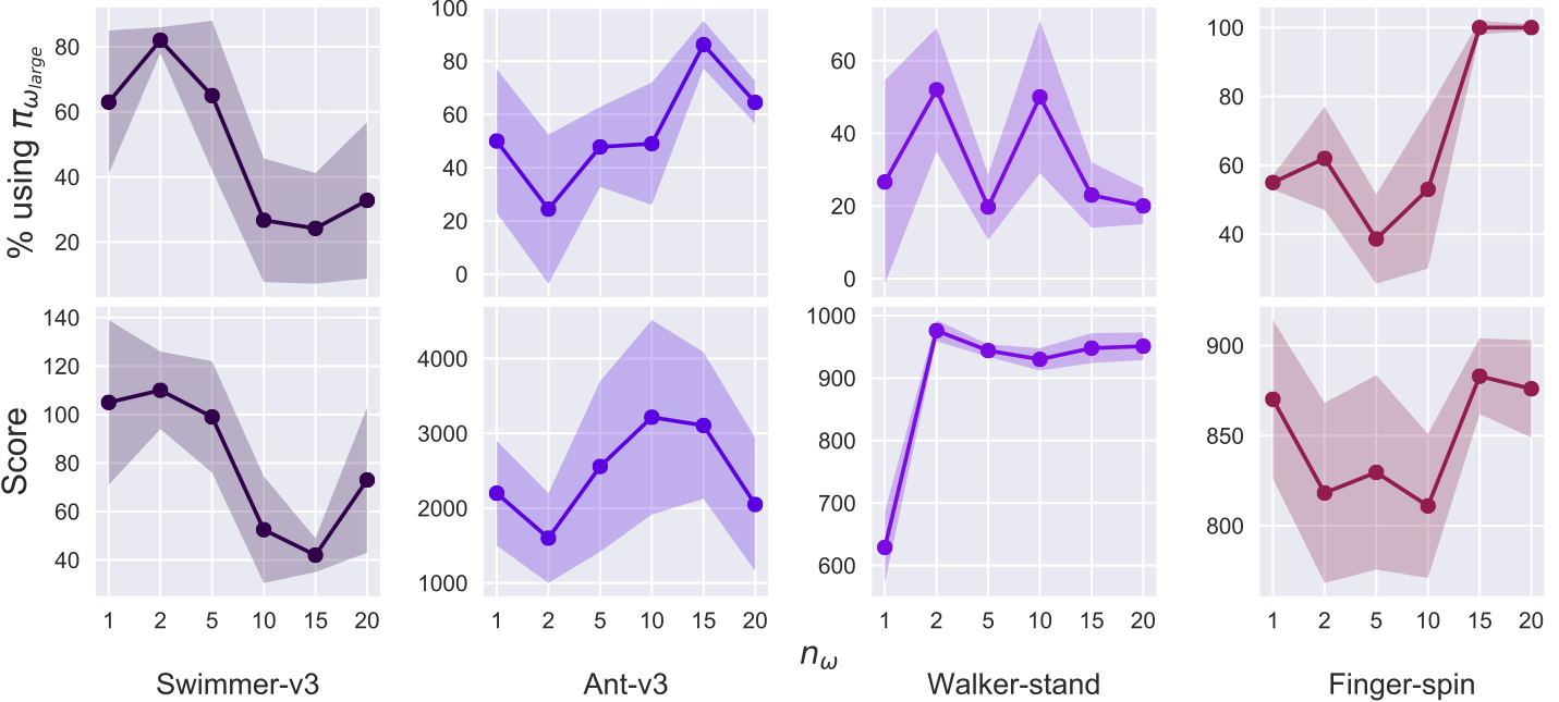
Figure 3: Performance of models trained with different $n_{\omega}$. The scores are averaged from 5 different random seeds. Each model trained with different random seed is evaluated over 200 episodes.

We also do hyperparameter searches to find $n_{\omega}$. It can be observed from Fig. 3 that there is no obvious correlation between $n_{\omega}$ and the performance. Swimmer-v3 performs well with smaller values of $n_{\omega}$, while walker-stand performs well with larger values of $n_{\omega}$. On the other hand, Ant-v3 performs well with $n_{\omega}$ equal to around $10$. Therefore, the choice of $n_{\omega}$ is relatively non-straightforward. We select the value of $n_{\omega}$ on account of two considerations: (1) $n_{\omega}$ should not be too small, or it will lead to increased master policy costs due to more frequent inferences of the master policy to decide which sub-policy to be used next; (2) $n_{\omega}$ should not be too large, otherwise the model will not be able to perform flexible switching between sub-policies. As a result, we set $n_{\omega}$ to five for all of the experiments considered in this work as a compromise. However, please note that an adaptive scheme of the step size $n_{\omega}$ may potentially further enhance the overall performance, and is left as a future research direction.

For FetchPickAndPlace-v1, we train the model with hindsight experience replay (HER) [26] to improve the sample efficiency. For most of the results, the default training and evaluation lengths are set to 2.5M timesteps and 200 episodes, respectively. The agents are implemented based on the source codes from Stable Baselines [27] as well as RL Baselines Zoo [28], and are trained using five different random seeds.

V-A3 Baselines

The baselines considered include two categories: (1) a typical RL method, and (2) distillation methods.

Typical RL method. To study the performance drop and the cost reduction compared with standard RL methods, we train two policies of different sizes (i.e., numbers of DNN parameters), where the small one and the large one are denoted as $\pi_{S-only}$ and $\pi_{L-only}$ respectively. The sizes of $\pi_{S-only}$ and $\pi_{L-only}$ correspond to $\pi_{\omega_{small}}$ and $\pi_{\omega_{large}}$ used in our method. Both $\pi_{S-only}$ and $\pi_{L-only}$ are trained independently from scratch as typical RL methods without the use of $\pi_{\Omega}$.

Distillation methods. In order to study the effectiveness on cost reduction, we compare our methodology with a commonly used method in RL: policy distillation. Two policy distillation approaches are considered in our experiments: Behavior Cloning (BC) [29] and Generative Adversarial Imitation Learning (GAIL) [30]. For these baselines, a costly policy (i.e., the large policy) serves as the teacher model that distills its policy to an economic policy (i.e., the small policy). In our experiments, the teacher network is set to $\pi_{{L-only}}$, while the configurations of the student networks are described in Section V-D. Please note that these baselines require more training data than the typical RL method baselines and our methodology, since they need data samples from expert (i.e., $\pi_{{L-only}}$) trajectories for training their student networks.

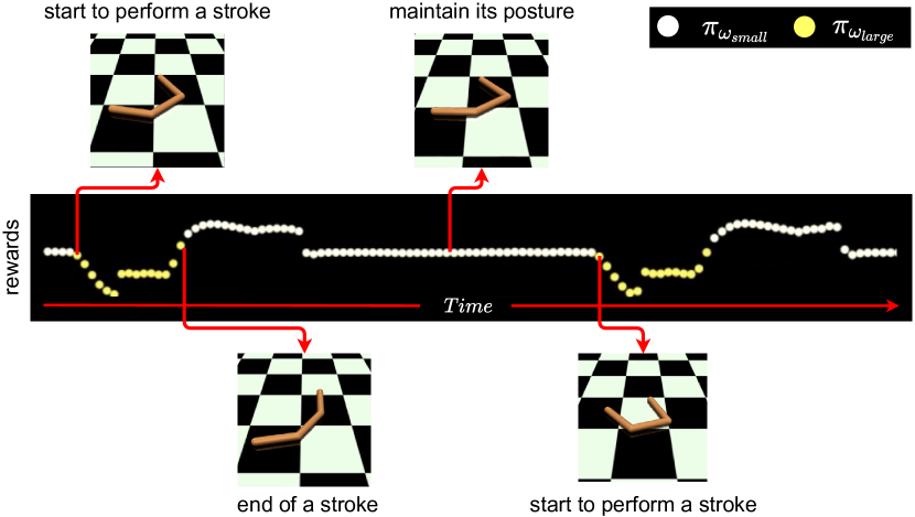
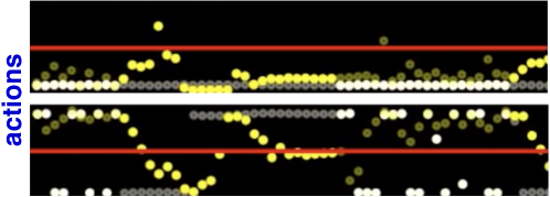
Figure 4: A timeline for illustrating the sub-policies used for different circumstances in Swimmer-v3, where the interleavedly plotted white and yellow dots along the timeline correspond to the sub-policies $\pi_{\omega_{small}}$ and $\pi_{\omega_{large}}$, respectively. The master policy $\pi_{\Omega}$ selects $\pi_{\omega_{large}}$ when performing strokes, and employs $\pi_{\omega_{small}}$ to maintain or slightly adjust the posture of the swimmer between two strokes for drifting. The image at the bottom shows the actions conducted by the model. The transparent dots are actions decided by the not selected sub-policy. The opaque and the transparent dots reveal that actions conducted by $\pi_{\omega_{large}}$ is more complicated than $\pi_{\omega_{small}}$.

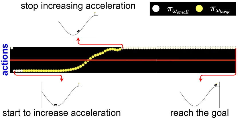
(a) MountainCarContinuous-v0

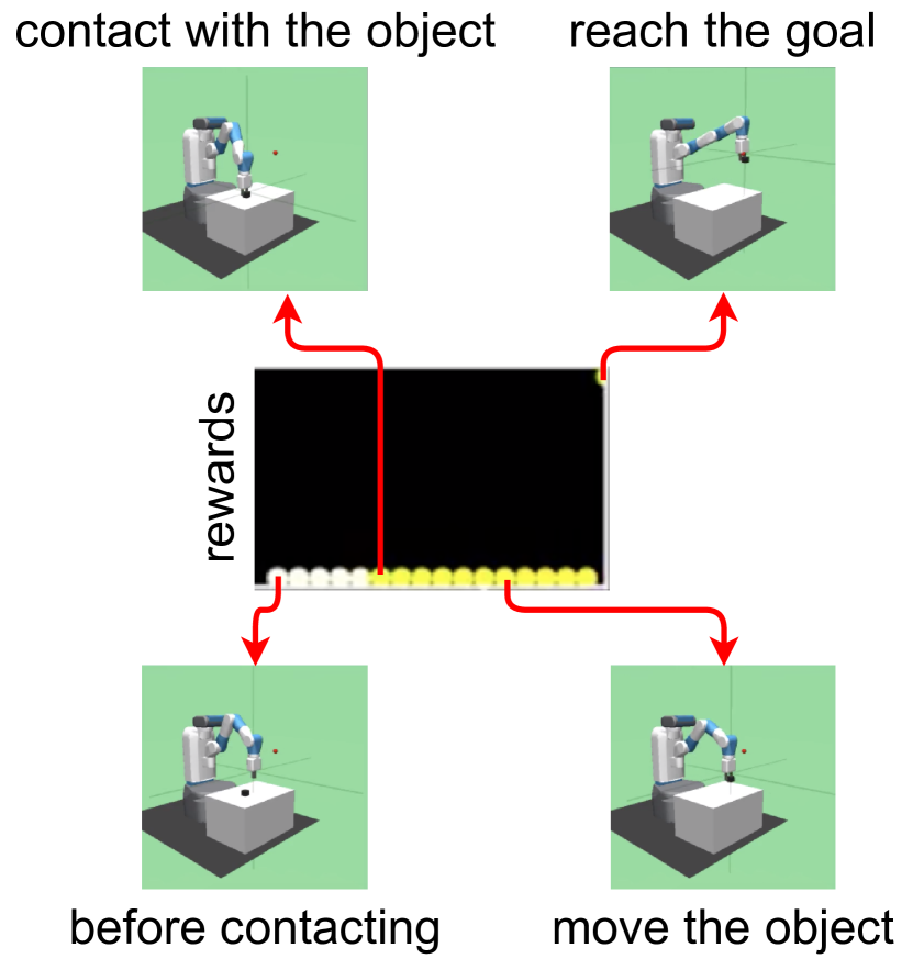
(b) FetchPickAndPlace-v1

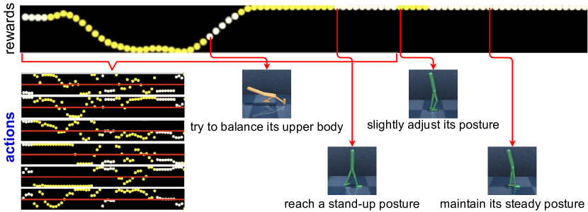
(c) Walker-stand

Figure 5: 5(a) The mountain car uses $\pi_{\omega_{large}}$ to adjust its acceleration from a negative value to a positive value, while using $\pi_{\omega_{small}}$ to maintain its acceleration. 5(b) The robotic arm first approaches the object using $\pi_{\omega_{small}}$, and then employs $\pi_{\omega_{large}}$ to move the object to the target location. 5(c) The walker first utilizes $\pi_{\omega_{large}}$ and $\pi_{\omega_{small}}$ alternately to stand up. After reaching an upright posture, the walker leverages $\pi_{\omega_{small}}$ to maintain it afterwards.

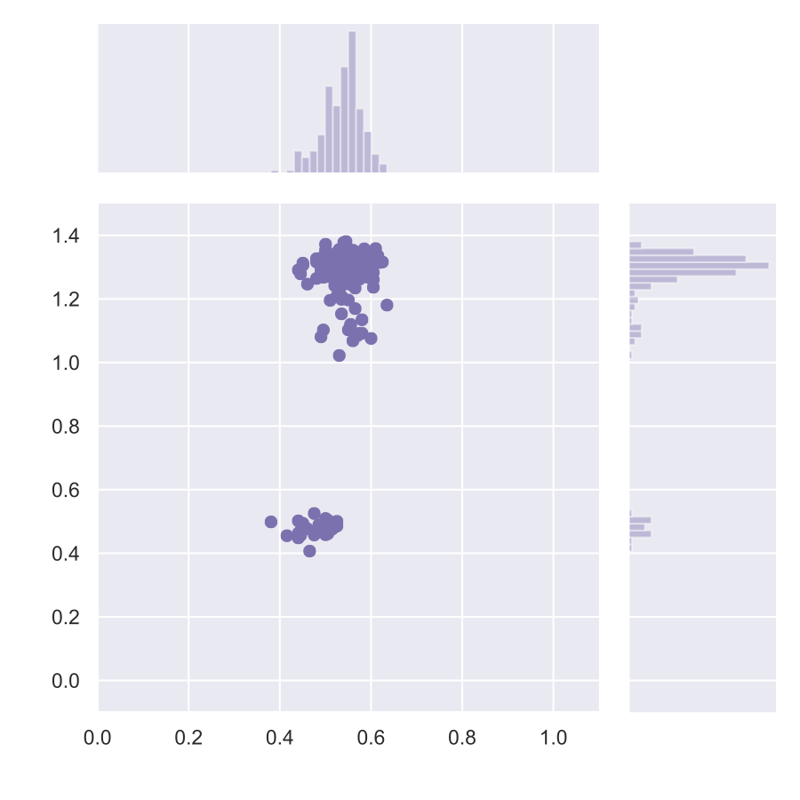
(a) Swimmer-v3

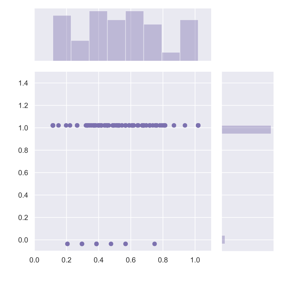
(b) FetchPickAndPlace-v1

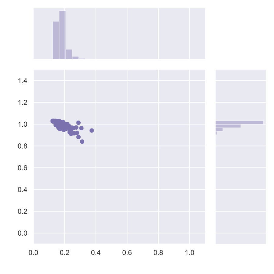
(c) walker-stand

                              Performance (scaled)

Inference costs (scaled)

Figure 6: Comparison of performance and cost. Each dot corresponds to a rollout of an episode. The $y$-axis is scaled so that the expert achieves 1 and a random policy achieves 0. The $x$-axis is also scaled such that only using $\pi_{\omega_{large}}$ throughout an episode corresponds to 1.

V-B Qualitative Analysis of the Learned Behaviors

We first illustrate a number of motivating timeline plots to qualitatively demonstrate that a control task can be handled by different sub-policies $\pi_{\omega}$ during different circumstances.

Swimmer-v3. Fig. 4 illustrates the decisions of the master policy $\pi_{\Omega}$, where the interleavedly plotted white and yellow dots along the timeline correspond to the execution of sub-policies $\pi_{\omega_{small}}$ and $\pi_{\omega_{large}}$, respectively. In this task, a swimmer robot is expected to first perform a stroke and then maintain a proper posture so as to drift for a longer distance. It is observed that the model trained by our methodology tends to use $\pi_{\omega_{large}}$ while performing strokes and $\pi_{\omega_{small}}$ to maintain its posture between two strokes. One reason is that a successful stroke requires lots of delicate changes in each joint while holding a proper posture for drifting merely needs a few joint changes. Delicate changes in posture within a small time interval are difficult for $\pi_{\omega_{small}}$ since the outputs of it tend to be smooth over temporally neighboring states.

MountainCarContinuous-v0. The objective of the car is to reach the flag at the top of the hill on the right-hand side. In order to reach the goal, the car has to accelerate forward and backward and then stop acceleration at the top. Fig. 5(a) shows that $\pi_{\omega_{large}}$ is used for adjusting the acceleration and $\pi_{\omega_{small}}$ is only selected when acceleration is not required.

FetchPickAndPlace-v1. The goal of the robotic arm is to move the black object to a target position (i.e., the red ball in Fig. 5(b)). In Fig. 5(b), it can be observed that the agent trained by our methodology learns to use $\pi_{\omega_{small}}$ to approach the object, and then switch to $\pi_{\omega_{large}}$ to fetch and move it to the target location. One rationale for this observation is that fetching and moving an object entails fine-grained control of the clipper. The need for fine-grained control inhibits $\pi_{\omega_{small}}$ from being selected by $\pi_{\Omega}$ to fetch and move objects. In contrast, there is no need for fine-grained control for approaching objects. As a result, $\pi_{\omega_{small}}$ is mostly chosen when the arm is approaching the object to reduce the costs.

Walker-stand. The goal of the walker is to stand up and maintain an upright torso. Fig. 5(c) shows that for circumstances when the forces applied change quickly, $\pi_{\omega_{large}}$ is used. For circumstances where the forces applied change slowly, $\pi_{\omega_{small}}$ is used. After the walker reaches a balanced posture, it utilizes $\pi_{\omega_{small}}$ to maintain the posture afterwards.

To summarize the above findings, $\pi_{\omega_{large}}$ is selected when find-grained controls (i.e., tweaking actions within a small time interval) are necessary, and $\pi_{\omega_{small}}$ is chosen otherwise.

TABLE III: A summary of the performances of $\pi_{{S-only}}$, $\pi_{{L-only}}$, and our method (denoted as ‘Ours’) evaluated over 200 test episodes, along with the averaged percentages of $\pi_{\omega_{large}}$ being used by our method during an episode, as well as the averaged percentages of reduction in FLOPs when comparing Ours (including the FLOPs from $\pi_{\Omega}$ and the sub-policies) against $\pi_{{L-only}}$.

Environment	$\pi_{{S-only}}$	$\pi_{{L-only}}$	Ours	% using $\pi_{\omega_{large}}$	% Total FLOPs reduction
MountainCarContinuous-v0	$-11.6\pm 0.1$	$93.6\pm 0.1$	$93.5\pm 0.1$	$44.5\%\pm 5.7\%$	$49.0\%\pm 5.3\%$
Swimmer-v3	$35.5\pm 7.7$	$84.1\pm 18.0$	$108.8\pm 24.9$	$54.9\%\pm 9.5\%$	$44.6\%\pm 8.3\%$
Ant-v3	$1,690.4\pm 1,244.3$	$3,927.2\pm 1,602.8$	$3,564.8\pm 1,548.6$	$53.9\%\pm 5.5\%$	$39.3\%\pm 7.5\%$
FetchPickAndPlace-v1	$0.351\pm 0.477$	$0.980\pm 0.140$	$0.935\pm 0.255$	$46.5\%\pm 3.0\%$	$46.4\%\pm 2.8\%$
walker-stand	$330.0\pm 12.2$	$977.7\pm 22.1$	$967.2\pm 16.4$	$5.7\%\pm 1.1\%$	$82.3\%\pm 0.9\%$
finger-spin	$32.9\pm 36.9$	$978.0\pm 32.4$	$871.2\pm 24.0$	$55.2\%\pm 19.7\%$	$37.5\%\pm 17.8\%$

V-C Performance and Cost Reduction

In this section, we compare the performance and the cost of our method with typical RL methods described in Section V-A. Table III summarizes the performances corresponding to $\pi_{{S-only}}$, $\pi_{{L-only}}$, and our method (denoted as ‘Ours’) in the second, third, and fourth columns, respectively. Table III also summarizes the averaged percentages of $\pi_{\omega_{large}}$ being used by our method during an episode, as well as the averaged percentages of reduction in FLOPs when comparing Ours (including the FLOPs from the master policy $\pi_{\Omega}$ as well as the two sub-policies) against the $\pi_{{L-only}}$ baseline.

It can be seen that in Table III, the average performance of Ours are comparable to $\pi_{L-only}$ and significantly higher than $\pi_{S-only}$. It can also be observed that our method does switch between $\pi_{\omega_{small}}$ and $\pi_{\omega_{large}}$ to control the agent, and thus reduce the total cost required for solving the tasks.

To take a closer look into the behavior of the agent within an episode, Fig. 6 illustrates the performances and costs of our methodology over 200 episodes during evaluation for three control tasks. Each dot plotted in Fig. 6 corresponds to the evaluation result of Ours in an episode, where the cost of each dot is divided by the cost of $\pi_{{L-only}}$. The performance of each dot is also scaled such that $[0,1]$ corresponds to the averaged performances of a random policy and $\pi_{{L-only}}$. Please note that the scaled costs of our methodology may exceed one since the inference costs of $\pi_{\Omega}$ are considered in our statistics as well. Histograms corresponding to the performances and costs of the data points are provided on the right-hand side and the top side of each figure, respectively. For Swimmer-v3, it is observed that our methodology is able to reduce about half of the FLOPs when compared against $\pi_{{L-only}}$. Although few data points correspond to only half of the averaged performance of $\pi_{{L-only}}$, most of the data points are comparable and even superior to that. For FetchPickAndPlace-v1, it can be observed that the dots distribute evenly along the line (y=1.0), which means that the agent can solve the tasks in the majority of episodes while the induced costs vary largely across episodes. This phenomena is mainly caused by the broadly varying starting positions in different episodes. When the object is close the arm, the cost is near 1.0 since $\pi_{\omega_{large}}$ is used in the majority of time in an episode, as the result shown in Section V-B. For walker-stand, our method learns to use $\pi_{\omega_{large}}$ in the early stages to control the walker to stand up. After that, the agent only uses $\pi_{\omega_{small}}$ to slightly adjust its joints to maintain the posture of the walker. Therefore, a significant amount of inference costs can be saved in this task, causing the data points to concentrate on the top-left corner of the figure. These examples therefore validate that our cost-aware methodology is able to provide sufficient performances while reducing the inference costs required for completing the tasks.

V-D Analysis of the Performance and the FLOPs per Inference

TABLE IV: An analysis of the performances and FLOPs per inference (denoted as FLOPs/Inf) for our method and the baselines. The network sizes of $\pi_{{fit}}$ and the student networks of the two policy distillation baselines are configured such that their FLOPs/Inf are approximately the same as the averaged FLOPs/Inf of Ours (denoted as Avg-FLOPs/Inf). In MountainCarContinuous-v0, $\pi_{{L-only}}$, Ours, and $\pi_{{fit}}$ are trained for 100k timesteps. In other control tasks, they are trained for 2M timesteps. BC and GAIL require additional expert trajectories generated by the trained model $\pi_{{L-only}}$, which consists of 25 trajectories with 50 state-action pairs for each trajectory, as adopted in [30]. Note that the numerical results presented in this table correspond to the score of best model selected from 5 training runs.

Environment	$\pi_{{L-only}}$	FLOPs/Inf	Ours	Avg-FLOPs/Inf	$\pi_{{fit}}$	GAIL	BC	FLOPs/Inf
MountainCarContinuous-v0	$93.6\pm 0.1$	8,707	$93.5\pm 0.1$	$4,440\pm 177$	$90.5\pm 0.1$	$-99.9\pm 0.0$	$93.3\pm 0.1$	4,603
Swimmer-v3	$84.1\pm 10.3$	137,219	$108.8\pm 15.4$	$76,019\pm 9,122$	$66.2\pm 10.1$	$63.2\pm 9.8$	$59.7\pm 13.8$	76,763
Ant-v3	$3,927.2\pm 524.0$	196,099	$3,564.8\pm 724.7$	$119,032\pm 14,284$	$2,553.0\pm 511.7$	$-15.6\pm 101.0$	$1,373.7\pm 490.2$	119,451
FetchPickAndPlace-v1	$0.980\pm 0.140$	42,755	$0.935\pm 0.247$	$22,917\pm 2,521$	$0.920\pm 0.271$	$0.078\pm 0.268$	$0.153\pm 0.360$	23,223
walker-stand	$977.7\pm 20.2$	12,803	$967.2\pm 16.3$	$2,266\pm 159$	$819.5\pm 14.5$	$596.6\pm 33.9$	$159.1\pm 22.6$	2,397
finger-spin	$978.0\pm 33.0$	9,859	$871.2\pm 28.5$	$6,162\pm 739$	$848.1\pm 27.0$	$536.8\pm 22.4$	$7.6\pm 19.5$	6,303

TABLE V: Comparison of the proposed methodology with and without using the cost term $c_{\omega}$.

	With the cost term $c_{\omega}$		Without the cost term $c_{\omega}$
Environment	Performance	% using $\pi_{\omega_{large}}$	Performance	% using $\pi_{\omega_{large}}$
MountainCarContinuous-v0	$35.5\pm 48.9$	$50.4\%\pm 5.5\%$	$66.3\pm 40.6$	$59.0\%\pm 20.5\%$
Swimmer-v3	$98.9\pm 23.2$	$65.2\%\pm 15.0\%$	$71.5\pm 33.3$	$99.5\%\pm 1.1\%$
Ant-v3	$2,558.8\pm 1140.0$	$47.8\%\pm 15.0\%$	$2,625.8\pm 728.6$	$80.9\%\pm 39.2\%$
FetchPickAndPlace-v1	$0.822\pm 0.103$	$51.3\%\pm 13.8\%$	$0.785\pm 0.175$	$44.2\%\pm 16.0\%$
walker-stand	$943.8\pm 23.3$	$19.7\%\pm 9.8\%$	$961.8\pm 10.0$	$100.0\%\pm 0.0\%$
finger-spin	$829.6\pm 54.2$	$38.6\%\pm 14.9\%$	$907.4\pm 29.7$	$100.0\%\pm 0.0\%$

TABLE VI: Comparison of our methodology with and without a shared experience replay buffer.

	With shared $\mathcal{Z_{\omega}}$		Without shared $\mathcal{Z_{\omega}}$
Environment	Performance	% using $\pi_{\omega_{large}}$	Performance	% using $\pi_{\omega_{large}}$
MountainCarContinuous-v0	$35.5\pm 48.9$	$50.4\%\pm 5.5\%$	$0.0\pm 0.0$	$59.8\%\pm 54.6\%$
Swimmer-v3	$98.9\pm 23.2$	$65.2\%\pm 15.0\%$	$61.1\pm 23.6$	$50.8\%\pm 45.8\%$
Ant-v3	$2,558.8\pm 1,140.0$	$47.8\%\pm 15.0\%$	$1,270.1\pm 1,331.4$	$23.8\%\pm 42.6\%$
FetchPickAndPlace-v1	$0.822\pm 0.103$	$51.3\%\pm 13.8\%$	$0.377\pm 0.128$	$63.0\%\pm 17.4\%$
Walker-stand	$943.8\pm 23.3$	$19.7\%\pm 9.8\%$	$910.1\pm 65.9$	$25.1\%\pm 31.1\%$
Finger-spin	$829.6\pm 54.2$	$38.6\%\pm 14.9\%$	$865.9\pm 41.8$	$70.7\%\pm 20.6\%$

We compare the performances of the proposed methodology and the baselines discussed in Section V-A3, as well as their FLOPs per inference (denoted as FLOPs/Inf). The FLOPs/Inf for $\pi_{{L-only}}$, Ours, and the student networks of the baselines, as well as their corresponding highest performances achieved are summarized in Table IV. For a fair comparison, the sizes of the student networks of the distillation baselines are configured such that their FLOPs/Inf (the last column of Table IV) are approximately the same as the averaged FLOPs/Inf of Ours (the Avg-FLOPs/Inf column in Table IV, including the FLOPs contributed by both the master policy $\pi_{\Omega}$ and the sub-policies). As a reference, we additionally train a policy $\pi_{{fit}}$ using SAC from scratch based on the same DNN size as the student networks of the distillation baselines. For distillation baselines, both of them employ the pre-trained $\pi_{{L-only}}$ as their teacher networks. Then, the student networks are trained using the data sampled from the trajectories generated by the teacher networks, where 50 consecutive state-action pairs are sampled from each of the generated 25 trajectories, as those adopted in [30].

The results show that for the environments in Table IV, Ours deliver comparable performances to the $\pi_{{L-only}}$ baseline and outperforms the distillation baselines, under similar levels of FLOPs/Inf. From the perspective of data samples used, the distillation baselines consume more data samples (including the data samples required for training both the teacher and the student networks) than those required by Ours, which is trained from scratch without the need of data samples from a pre-trained teacher network. The relatively lower performances of the distillation baselines are probably due to the smaller sizes of the networks compared to their teacher networks $\pi_{{L-only}}$, since the performances delivered by $\pi_{{fit}}$ are also lower than the corresponding performances of Ours. The results thus suggest that our method is able to reduce inference costs while maintaining sufficient performances.

V-E Ablation Study

Effectiveness of the cost term. We compare the evaluation results of our models trained with and without using the loss term in Table V. When the cost term is removed, the main factor that affects the decisions of $\pi_{\Omega}$ is its belief in how good each sub-policy can achieve. Since $\pi_{\omega_{large}}$ is able to obtain high scores on its own, it is observed that $\pi_{\Omega}$ prefers to select $\pi_{\omega_{large}}$. In contrast, incorporating the cost term decreases the percentages of using $\pi_{\omega_{large}}$ substantially, while still allowing our model to offer satisfying performances.

Effectiveness of shared experience replay buffer. We compare the results of our models with and without the shared buffer across sub-policies $\pi_{\omega}$ in Table VI. For tasks except finger-spin, the scores of the models without a shared $\mathcal{Z_{\omega}}$ are lower than those with a shared $\mathcal{Z_{\omega}}$. The lower scores of the models are due to reduced data samples for each sub-policies, since the transitions are not shared across the replay buffers. We also observed that some of the model trained without a shared $\mathcal{Z_{\omega}}$ is prone to use one of its sub-policies for the majority of time, instead of using both interleavedly. We believe that this is caused by unbalanced training samples for the two sub-policies. Namely, the relatively worse sub-policy is less likely to obtain sufficient data samples to improve its performance. While this problem can be solved by using training algorithms with improved exploration such as [2], we simply share $\mathcal{Z_{\omega}}$ among $\pi_{\omega}$ to address this issue. The models trained with a shared $\mathcal{Z_{\omega}}$ have lower variances in the choice of the two sub-policies (i.e., the third column of Table VI), and can exhibit more stable behaviors for $\pi_{\Omega}$.

VI Conclusion

We proposed a methodology for performing cost-aware control based on an asymmetric architecture. Our methodology uses a master policy to select between a large sub-policy network and a small sub-policy network. The master policy is trained to take inference costs into its consideration, such that the two sub-policies are used alternately and cooperatively to complete the task. The proposed methodology is validated in a wide set of control environments and the quantitative and qualitative results presented in this paper show that the proposed methodology provides sufficient performances while reducing the inference costs required. The comparison of the proposed methodology and the baseline methods indicated that the proposed methodology is able to deliver comparable performance to the $\pi_{{L-only}}$ baseline, while requiring less training data than the knowledge distillation baselines.

References

- [1] V. Mnih, K. Kavukcuoglu, and D. e. a. Silver, “Human-level control through deep reinforcement learning,” Nature, vol. 518, no. 7540, pp. 529–533, 2015.
- [2] V. Mnih, A. P. Badia, M. Mirza, A. Graves, T. P. Lillicrap, T. Harley, D. Silver, and K. Kavukcuoglu, “Asynchronous methods for deep reinforcement learning,” 2016.
- [3] D. Silver, A. Huang, C. J. Maddison, A. Guez, L. Sifre, G. van den Driessche, J. Schrittwieser, I. Antonoglou, V. Panneershelvam, M. Lanctot, S. Dieleman, D. Grewe, J. Nham, N. Kalchbrenner, I. Sutskever, T. Lillicrap, M. Leach, K. Kavukcuoglu, T. Graepel, and D. Hassabis, “Mastering the game of go with deep neural networks and tree search,” Nature, vol. 529, no. 7587, pp. 484–489, 2016. [Online]. Available: https://doi.org/10.1038/nature16961
- [4] T. P. Lillicrap, J. J. Hunt, A. Pritzel, N. M. O. Heess, T. Erez, Y. Tassa, D. Silver, and D. Wierstra, “Continuous control with deep reinforcement learning,” CoRR, vol. abs/1509.02971, 2015.
- [5] T. Haarnoja, A. Zhou, P. Abbeel, and S. Levine, “Soft actor-critic: Off-policy maximum entropy deep reinforcement learning with a stochastic actor,” ArXiv, vol. abs/1801.01290, 2018.
- [6] S. Gu, E. Holly, T. Lillicrap, and S. Levine, “Deep reinforcement learning for robotic manipulation with asynchronous off-policy updates,” in ICRA, 05 2017, pp. 3389–3396.
- [7] Synced. (2017) Deep learning in real time — inference acceleration and continuous training. [Online]. Available: https://medium.com/syncedreview/deep-learning-in-real-time-inference-acceleration-and-continuous-training-17dac9438b0b
- [8] V. Sze, Y.-H. Chen, T.-J. Yang, and J. Emer, “Efficient processing of deep neural networks: A tutorial and survey,” Proceedings of the IEEE, vol. 105, 03 2017.
- [9] R. S. Sutton, “Between mdps and semi-mdps: A framework for temporal abstraction in reinforcement learning,” Artif. Intell., vol. 112, no. 1–2, p. 181–211, Aug. 1999. [Online]. Available: https://doi.org/10.1016/S0004-3702(99)00052-1
- [10] G. Brockman, V. Cheung, L. Pettersson, J. Schneider, J. Schulman, J. Tang, and W. Zaremba, “Openai gym,” 2016.
- [11] Y. Tassa, Y. Doron, A. Muldal, T. Erez, Y. Li, D. de Las Casas, D. Budden, A. Abdolmaleki, J. Merel, A. Lefrancq, T. Lillicrap, and M. Riedmiller, “DeepMind control suite,” https://arxiv.org/abs/1801.00690, DeepMind, Tech. Rep., Jan. 2018. [Online]. Available: https://arxiv.org/abs/1801.00690
- [12] G. Hinton, O. Vinyals, and J. Dean, “Distilling the knowledge in a neural network,” in NIPS Deep Learning and Representation Learning Workshop, 2015. [Online]. Available: http://arxiv.org/abs/1503.02531
- [13] A. Romero, N. Ballas, S. E. Kahou, A. Chassang, C. Gatta, and Y. Bengio, “Fitnets: Hints for thin deep nets,” 2014.
- [14] J. Ba and R. Caruana, “Do deep nets really need to be deep?” in Advances in Neural Information Processing Systems 27, Z. Ghahramani, M. Welling, C. Cortes, N. D. Lawrence, and K. Q. Weinberger, Eds. Curran Associates, Inc., 2014, pp. 2654–2662. [Online]. Available: http://papers.nips.cc/paper/5484-do-deep-nets-really-need-to-be-deep.pdf
- [15] H. Tann, S. Hashemi, R. I. Bahar, and S. Reda, “Hardware-software codesign of accurate, multiplier-free deep neural networks,” in 2017 54th ACM/EDAC/IEEE Design Automation Conference (DAC), 2017, pp. 1–6.
- [16] C. Florensa, Y. Duan, and P. Abbeel, “Stochastic neural networks for hierarchical reinforcement learning,” ICLR, 04 2017.
- [17] P.-L. Bacon, J. Harb, and D. Precup, “The option-critic architecture,” 2016.
- [18] O. Nachum, S. Gu, H. Lee, and S. Levine, “Data-efficient hierarchical reinforcement learning,” 2018.
- [19] A. S. Vezhnevets, S. Osindero, T. Schaul, N. Heess, M. Jaderberg, D. Silver, and K. Kavukcuoglu, “Feudal networks for hierarchical reinforcement learning,” in Proceedings of the 34th International Conference on Machine Learning - Volume 70, ser. ICML’17. JMLR.org, 2017, p. 3540–3549.
- [20] C. Tessler, S. Givony, T. Zahavy, D. J. Mankowitz, and S. Mannor, “A deep hierarchical approach to lifelong learning in minecraft,” in Proceedings of the Thirty-First AAAI Conference on Artificial Intelligence, ser. AAAI’17. AAAI Press, 2017, p. 1553–1561.
- [21] J. Andreas, D. Klein, and S. Levine, “Modular multitask reinforcement learning with policy sketches,” in Proceedings of the 34th International Conference on Machine Learning - Volume 70, ser. ICML’17. JMLR.org, 2017, p. 166–175.
- [22] J. Harb, P.-L. Bacon, M. Klissarov, and D. Precup, “When waiting is not an option : Learning options with a deliberation cost,” in AAAI, 2018.
- [23] M. Hessel, H. Soyer, L. Espeholt, W. Czarnecki, S. Schmitt, and H. van Hasselt, “Multi-task deep reinforcement learning with popart,” DeepMind, Tech. Rep., 2019. [Online]. Available: https://www.aaai.org/ojs/index.php/AAAI/article/view/4266
- [24] A. Li, C. Florensa, I. Clavera, and P. Abbeel, “Sub-policy adaptation for hierarchical reinforcement learning,” in ICLR, 2020.
- [25] E. Todorov, T. Erez, and Y. Tassa, “Mujoco: A physics engine for model-based control,” in 2012 IEEE/RSJ International Conference on Intelligent Robots and Systems, Oct 2012, pp. 5026–5033.
- [26] M. Andrychowicz, F. Wolski, A. Ray, J. Schneider, R. Fong, P. Welinder, B. McGrew, J. Tobin, P. Abbeel, and W. Zaremba, “Hindsight experience replay,” in Proceedings of the 31st International Conference on Neural Information Processing Systems, ser. NIPS’17. Red Hook, NY, USA: Curran Associates Inc., 2017, p. 5055–5065.
- [27] A. Hill, A. Raffin, M. Ernestus, A. Gleave, A. Kanervisto, R. Traore, P. Dhariwal, C. Hesse, O. Klimov, A. Nichol, M. Plappert, A. Radford, J. Schulman, S. Sidor, and Y. Wu, “Stable baselines,” https://github.com/hill-a/stable-baselines, 2018.
- [28] A. Raffin, “Rl baselines zoo,” https://github.com/araffin/rl-baselines-zoo, 2018.
- [29] F. Codevilla, E. Santana, A. Lopez, and A. Gaidon, “Exploring the limitations of behavior cloning for autonomous driving,” in 2019 IEEE/CVF International Conference on Computer Vision (ICCV), 2019, pp. 9328–9337.
- [30] J. Ho and S. Ermon, “Generative adversarial imitation learning,” 2016.