Occam Learning Meets Synthesis Through Unification

Abstract.

The generalizability of PBE solvers is the key to the empirical synthesis performance. Despite the importance of generalizability, related studies on PBE solvers are still limited. In theory, few existing solvers provide theoretical guarantees on generalizability, and in practice, there is a lack of PBE solvers with satisfactory generalizability on important domains such as conditional linear integer arithmetic (CLIA). In this paper, we adopt a concept from the computational learning theory, Occam learning, and perform a comprehensive study on the framework of synthesis through unification (STUN), a state-of-the-art framework for synthesizing programs with nested if-then-else operators. We prove that Eusolver, a state-of-the-art STUN solver, does not satisfy the condition of Occam learning, and then we design a novel STUN solver, PolyGen, of which the generalizability is theoretically guaranteed by Occam learning. We evaluate PolyGen on the domains of CLIA and demonstrate that PolyGen significantly outperforms two state-of-the-art PBE solvers on CLIA, Eusolver and Euphony, on both generalizability and efficiency.

1. Introduction

In the past decades, oracle-guided inductive program synthesis (OGIS) (Jha and Seshia, 2017) receives much attention. In each iteration of OGIS, an oracle provides input-output examples to an inductive program synthesizer, or programming-by-example (PBE) synthesizer (Shaw et al., 1975), and the PBE synthesizer generates a program based on the examples. There are two typical types of OGIS problems. In the first type, the oracle can verify whether the synthesized program is correct, and provides a counter-example if the program is incorrect. Many applications under the counter-example guided inductive synthesis (CEGIS) framework (Solar-Lezama et al., 2006) fall into this type. In the second type, the oracle cannot verify the correctness of the synthesized program but can provide a set of input-output examples. This includes the applications where the oracle is a black-box program, such as binary programs (Zhai et al., 2016), and applications where the program is too complex to verify its correctness, e.g., the task involves system calls or complex loops, such as program repair, second-order execution, and deobfuscation (Mechtaev et al., 2015a; Mechtaev et al., 2018; David et al., 2020; Blazytko et al., 2017; Jha et al., 2010).

In both types of problems, the generalizability of the PBE solver is the key to synthesis performance. In the first type, generalizability significantly affects the efficiency: the fewer examples the solver needs to synthesize a correct program, the fewer CEGIS iterations the synthesis requires, and thus the faster the synthesis would be. In the second type, the generalizability of the PBE solver decides the correctness of the whole OGIS system.

Despite the importance of generalizability, the studies on the generalizability of the existing PBE solvers are still limited. On the theoretical side, as far as we are aware, no existing PBE solver provides theoretical guarantees on generalizability. On the practical side, the generalizability of the existing PBE solvers is not satisfactory. As our evaluation will demonstrate later, on a synthesis task for solving the maximum segment sum problem, Eusolver (Alur et al., 2017), a state-of-the-art PBE solver, uses $393$ examples to find the correct program, while our solver uses only $10$.

In this paper, we propose a novel PBE solver, PolyGen, that provides a theoretical guarantee on generalizability by construction. We adopt a concept from the computational learning theory, Occam learning (Blumer et al., 1987), and prove that PolyGen is an Occam solver, i.e., a PBE solver that satisfies the condition of Occam learning. A PBE solver is an Occam solver if, for any possible target program consistent with the given examples, the size of the synthesized program is guaranteed to be polynomial to the target program and sub-linear to the number of provided examples with a high probability. In other words, an Occam solver would prefer smaller programs to larger programs and thus follows the principle of Occam’s Razor. In theory, Blumer et al. (1987) have proved that, given any expected accuracy, the number of examples needed by an Occam solver to guarantee the accuracy is bounded by a polynomial on the size of the target program. In practice, Occam learning has exhibited good generalizability in different domains (Kearns and Li, 1988; Kearns and Schapire, 1994; Angluin and Laird, 1987; Natarajan, 1993; Aldous and Vazirani, 1995).

PolyGen follows the synthesis through unification (STUN) (Alur et al., 2015) framework. STUN is a framework for synthesizing nested if-then-else programs, and the solvers based on STUN such as Eusolver (Alur et al., 2017) and Euphony (Lee et al., 2018) achieve the state-of-the-art results on many important benchmarks, e.g., the CLIA track in the SyGuS competition. A typical STUN solver consists of a term solver and a unifier. First the term solver synthesizes a set of if-terms, each being correct for a different subset of the input space, and then the unifier synthesizes if-conditions that combine the terms with if-then-else into a correct program for the whole input space.

We first analyze a state-of-the-art STUN solver, Eusolver (Alur et al., 2017), and prove that Eusolver is not an Occam solver. Then we proceed to design PolyGen. A key challenge to design an Occam solver is to scale up while satisfying the condition of Occam learning. For example, a trivial approach to ensuring Occam learning is to enumerate programs from small to large, and returns the first program consistent with the examples. However, this approach only scales to small programs. To ensure scalability, we divide the synthesis task into subtasks each synthesizing a subpart of the program, and propagate the condition of Occam learning into a sufficient set of conditions, where each condition is defined on a subtask. Roughly, these conditions require that each subtask synthesizes either a small program or a set of programs whose total size is small. Then, we find efficient synthesis algorithms that meet the respective conditions for each subtask.

We instantiate PolyGen on the domains of conditional linear integer arithmetic (CLIA), and evaluate PolyGen against Esolver (Alur et al., 2013), the best known PBE solver on CLIA that always synthesizes the smallest valid program, Eusolver (Alur et al., 2017) and Euphony (Lee et al., 2018), two state-of-the-art PBE solvers on CLIA. Our evaluation is conducted on $100$ benchmarks collected from the dataset of SyGuS-Comp (Alur et al., 2019) and an application of synthesizing divide-and-conquer algorithms (Farzan and Nicolet, 2017). Besides, our evaluation considers two major oracle models in OGIS, corresponding to the applications where (1) the oracle can provide a counter-example for a given program, and (2) the oracle can only generate the correct output for a given input. Our evaluation results show that:

• Comparing with Esolver, PolyGen achieves almost the same generalizability while solving 9.55 times more benchmarks than Esolver.

• Comparing with Eusolver and Euphony, on efficiency, PolyGen solves 43.08%-79.63% more benchmarks with $\times$7.02 - $\times$15.07 speed-ups. Besides, on generalizability, Eusolver and Euphony requires $\times$1.12 - $\times$2.42 examples comparing with PolyGen on those jointly solved benchmarks. This ratio raises to at least $\times$2.39 - $\times$3.33 when all benchmarks are considered.

To sum up, this paper makes the following contributions:

• We adopt the concept of Occam learning to the domain of PBE, prove that Eusolver is not an Occam solver, and provide a sufficient set of conditions for individual components in the STUN framework to form an Occam solver (Section 5).

• We design a novel Occam solver based on the STUN framework, PolyGen, by designing efficient algorithms for the two compoents that meet the above conditions. (Sections 6 and 7).

• We instantiate PolyGen to the domain of CLIA (Section 8) and evaluate PolyGen against state-of-the-art PBE solvers on CLIA (Section 9). The evaluation results show that PolyGen significantly outperforms Eusolver and Euphony on both efficiency and generalizability.

2. Related Work

Generalizability of PBE Solvers. Generalizability is known to be important for PBE solvers, and there have been different approaches proposed to improve generalizability.

Guided by the principle of Occam’s Razor, a major line of previous work converts the PBE task into an optimization problem by requiring the solver to find the simplest program (Liang et al., 2010; Gulwani, 2011; Raychev et al., 2016; Mechtaev et al., 2015b). This method has been evaluated to be effective in different domains, such as user-interacting PBE systems (Gulwani, 2011) and program repair (Mechtaev et al., 2015b). However, the usage of this method is limited by efficiency, as in theory, requiring the optimality of the solution would greatly increase the difficulty of a problem. For many important domains, there is still a lack of an efficient enough PBE solver which implementing this method. For example, on the domains of CLIA, our evaluation shows that Eusolver, a state-of-the-art PBE solver, solves $6.33$ times more benchmarks than Esolver (Alur et al., 2013), the known best PBE solver on CLIA that guarantees to return the simplest program.

Comparing with these previous work, though our paper is also based on the principle of Occam’s Razor, we relax the constraint on the PBE solver by adopting the concept of Occam Learning (Blumer et al., 1987) from computational learning theory. Occam learning allows the solver to return a program that is at most polynomially worse than the optimal and still has theoretical guarantees on generalizability. While designing an Occam solver, we have more space to improve the efficiency than designing a solver optimizing the size. In this way, we successfully implement a PBE solver on CLIA that performs well on both efficiency and generalizability.

Another line of work uses learned models to guide the synthesis procedure, and thus focuses on only probable programs (Balog et al., 2017; Kalyan et al., 2018; Ji et al., 2020; Singh and Gulwani, 2015; Chen et al., 2019; Menon et al., 2013; Devlin et al., 2017; Lee et al., 2018). However, the efficiency of these approaches depends on domain knowledge. For example, Kalyan et al. (2018) use input-output examples to predict the structure of the target program on the string manipulation domain: The effectiveness of their model relies on the structural information provided by strings and thus is unavailable on those unstructured domains, such as CLIA. In our evaluation, we evaluate a state-of-the-art PBE solver based on learned models, namely Euphony (Lee et al., 2018), and the result shows that its effectiveness is limited on CLIA.

Analysis on the generalizability. Analyzing the generalizability of learning algorithms is an important problem in machine learning and has been studied for decades. The probably approximately correct (PAC) learnability (Valiant, 1984) is a widely used framework for analyzing generalizability. When discussing PAC learnability of a learning task, the goal is to find a learning algorithm that (1) runs in polynomial time, (2) requires only a polynomial number of examples to achieve any requirement on the accuracy. On the synthesis side, there has been a line of previous work on the PAC learnability of logic programs (Cohen, 1995a, b; Dzeroski et al., 1992). Besides, some approaches use the framework of PAC learnability to analyze the number of examples required by some specific algorithm (Lau et al., 2003; Drews et al., 2019).

In this paper, we seek a theoretical model that can compare the generalizability of different PBE solvers. At this time, the requirement on the generalizability provided by PAC learnability is too loose: According to the general bound provided by Blumer et al. (1987), when the program space is finite, this condition is satisfied by any valid PBE solver. Therefore, we adopt another concept, Occam Learning, from computational learning theory. Comparing with PAC learnability, Occam learning (1) has a higher requirement on generalizability, as shown by Blumer et al. (1987), and (2) can reflect some empirical results in program synthesis, such as a PBE solver that always returns the simplest program should have better generalizability than an arbitrary PBE solver. To our knowledge, we are the first to introduce Occam Learning into program synthesis.

Synthesizing CLIA Programs. As mentioned in the introduction, our approach is implemented in the CLIA domain. CLIA is an important domain for program synthesis, as CLIA programs widely exist in real-world projects and can express complex behaviors by using nested if-then-else operators. There have been many applications of CLIA synthesizers, such as program repair (Mechtaev et al., 2015b; Le et al., 2017), automated parallelization (Farzan and Nicolet, 2017; Morita et al., 2007). On CLIA, PBE solvers are usually built on the STUN framework (Alur et al., 2015), which firstly synthesizes a set of if-terms by a term solver, and then unifies them into a program by a unifier. There are two state-of-the-art PBE solvers:

• Eusolver (Alur et al., 2017), which is comprised of an enumerative term solver and a unifier based on a decision-tree learning algorithm.

• Euphony (Lee et al., 2018), which uses structural probability to guide the synthesis of Eusolver.

PolyGen also follows the STUN framework. We evaluate PolyGen against these two solvers in Section 9. The result shows that PolyGen outperforms them on both efficiency and generalizability.

Outside PBE, there are other techniques proposed for synthesizing CLIA programs:

• DryadSynth (Huang et al., 2020) reconciles enumerative and deductive synthesis techniques. As DryadSynth requires a logic specificaion, it is not suitable for PBE tasks.

• CVC4 (Reynolds et al., 2019) synthesizes programs from unsatisfiability proofs given by theory solvers. Though CVC4 is runnable on PBE tasks, it seldom generalizes from examples. We test CVC4 on a simple task where the target is to synthesize a program that returns the maximal value among three inputs. After requiring $300$ random examples, the error rate of the program synthesized by CVC4 on a random input is still larger than $97\%$. In contrast, PolyGen requires only $12.2$ examples on average to synthesize a completely correct program.

There are also approaches on synthesizing boolean conditions, which is an important part in CLIA (Ernst et al., 2001; Padhi and Millstein, 2017). However, none of them discuss the theoretical guarantees on the generalizability, and it is unknown whether these approaches are Occam solvers.

3. Motivating Example and Approach Overview

In this section, we introduce the basic idea of our approach via a motivating example adopted from benchmark mpg_ite2.sl in the SyGuS competition. The target program $p^{*}$ is shown as the following, where $x,y,z$ are three integer inputs.

$$p^{*}(x,y,z)\coloneqq \texttt{ if }(x+y\geq 1)\texttt{ then }\{$$

$$\ \ \ \ \texttt{ if }(x+z\geq 1)\texttt{ then }\{x+1\}\texttt{ else }\{y+1\}$$

$$\texttt{ }\}\texttt{ else }\{$$

$$\ \ \ \ \texttt{ if }(y+z\geq 1)\texttt{ then }\{z+1\}\texttt{ else }\{y+1\}$$

$$\texttt{ }\}$$

We assume that there are $9$ input-output examples provided to the PBE solver. Table 1 lists these examples, where tuple $(x_{0},y_{0},z_{0})$ in column $I$ represents an input where $x,y,z$ are set to $x_{0},y_{0},z_{0}$ respectively, and the if-term in column Term represents the executed branch on each example.

Table 1. The input-output examples and the terms in the target program.

ID	$I$	$O$	Term	ID	$I$	$O$	Term	ID	$I$	$O$	Term
$e_{1}$	$(0,1,2)$	$1$	$x+1$	$e_{4}$	$(0,2,0)$	$3$	$y+1$	$e_{7}$	$(0,0,1)$	$2$	$z+1$
$e_{2}$	$(1,0,2)$	$2$		$e_{5}$	$(-1,3,0)$	$4$		$e_{8}$	$(-3,3,-2)$	$-1$
$e_{3}$	$(-1,3,2)$	$0$		$e_{6}$	$(-1,1,-1)$	$2$		$e_{9}$	$(-1,0,4)$	$5$

3.1. Eusolver

In this paper, we focus on designing an Occam solver for PBE tasks. As mentioned before, an Occam solver should synthesize programs whose size is polynomial to the size of the target program and sub-linear to the number of provided examples with high probability. Since the target program is unknown, an Occam solver should satisfy this requirement when the target program is the smallest valid program (programs consistent with the given input-output examples), and thus prefer smaller programs to larger programs.

We first show that Eusolver (Alur et al., 2017) may return unnecessarily large programs and thus is unlikely to be an Occam solver. We shall formally prove that Eusolver is not an Occam solver in Section 5.3. Eusolver follows the STUN framework and provides a term solver and an unifier. The term solver is responsible for synthesizing a term set that jointly covers all the given examples. In our example, one valid term set is $\{x+1,y+1,z+1\}$. A unifier is responsible for synthesizing a set of conditions to unify the term set into a program with nested if-then-else operators. In our example, the conditions are $\{x+y\geq 1,x+z\geq 1,y+z\geq 1\}$.

Similar to Occam learning, Eusolver also tries to return small programs. To achieve this, Eusolver enumerates the terms and the conditions from small to large, and then tries to combine the enumerated terms and conditions into a complete program. Though this approach controls the sizes of individual terms and conditions, it fails to control the number of the terms and the conditions, and thus may lead to unnecessarily large programs.

The term solver of Eusolver enumerates the terms from small to large, and includes a term in the term set when the set of examples covered by this term (i.e., the term is correct on these examples) is different from all smaller terms. The term set is complete when all examples are covered. As a result, this strategy may unnecessarily include many small terms, each covering only a few examples. In our motivating example, if constants such as $-1,\dots,5$ are available, $\mathcal{T}_{E}$ will return set $\{-1,\dots,5\}$ instead of $\{x+1,y+1,z+1\}$. Though such terms are small, the number of the terms grows with the number of examples.

The unifier of Eusolver builds a decision tree using the ID3 algorithms. Here the terms are considered as labels, the enumerated if-conditions are considered as conditions, and a term is a valid label for an example if it covers the example. However, ID3 is designed for fuzzy classification problems, uses information gain to select conditions, and may select conditions that negatively contribute to program synthesis. For example, $x\geq 0$ will have good information gain for this example. In the original sets the three labels $x+1$, $y+1$ and $z+1$ are evenly distributed. Predicate $x\geq 0$ divides the examples into two sets where the distribution become uneven: in one set 50% of the examples are labelled with $x+1$, and in the other set only 20% of the examples are labelled $x+1$. However, in both sets the three labels still exist, and we still have to find conditions to distinguish them. As a result, selecting $x>0$ roughly doubles the size of the synthesized program.

3.2. PolyGen

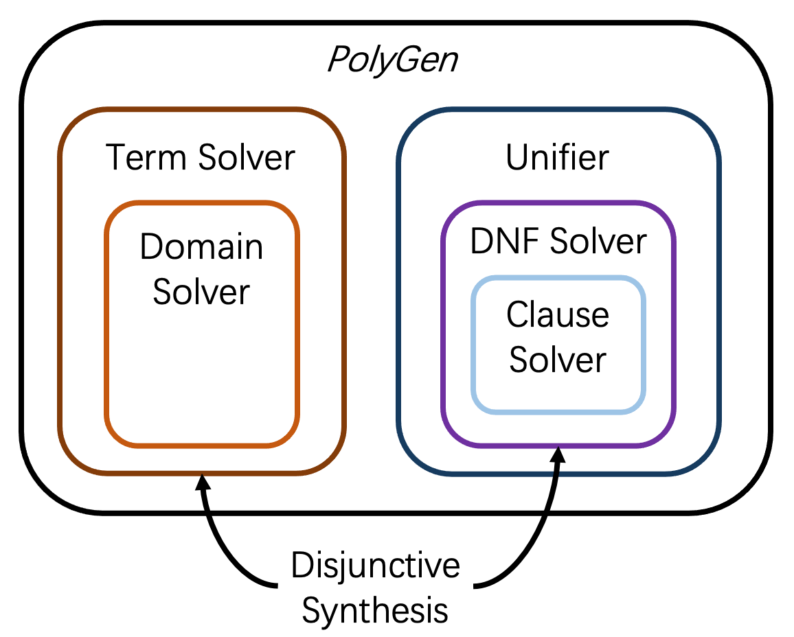
(a) The structure of PolyGen.

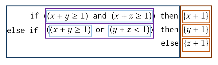
(b) The program synthesized by PolyGen from $\{e_{1},\dots,e_{9}\}$.

Figure 1. The left figure shows the structure of PolyGen, where each sub-solver in PolyGen is attached with a different color. The right figure shows the program synthesized by PolyGen from examples $\{e_{1},\dots,e_{9}\}$, where colored rectangles show the correspondence between partial programs and sub-solvers.

To synthesize small programs, PolyGen controls not only the size of individual terms and conditions but also the number of conditions and terms. The structure of PolyGen is shown as Figure 1(a). As we can see in the figure, PolyGen is built of a set of sub-solvers, each responsible for synthesizing part of the program. Figure 1(b) lists a program PolyGen synthesizes, and the colored rectangles show the parts of the program synthesized by the sub-solver with the same color. In the following we shall illustrate how PolyGen works.

3.2.1. Term Solver

To control the number of terms, the term solver of PolyGen iterates a threshold on the number of terms, and tries to synthesize a term set whose size is equal to or smaller than this threshold. The threshold starts with a small number, and increases by a constant $c$ in each iteration. The process terminates if any iteration successfully synthesizes a term set. In each iteration, PolyGen uses a randomized procedure to synthesize a term set. If a term set exists under a threshold, the probability that the term solver fails to synthesize a term set is bound by a constant $\epsilon$. Let us assume that a term set exists within the first iterated threshold. After $n$ iterations, the probability of failing to synthesize reduces to $\epsilon^{n}$, and the possible number of terms is only increased by $nc$. In other words, the number of the synthesized terms is guaranteed to be small with high probability.

Now we explain how we implement the randomized procedure to obtain a term set with a bounded failure probability. We assume there is a domain solver that synthesizes a term based on a set of examples, and the domain solver is also an Occam solver. For illustration, let us assume currently the threshold for the number of terms is 3, and in our example there exists at least one term set $T=\{x+1,y+1,z+1\}$ under this threshold. The term solver first samples many subsets of the examples and invoke the domain solver to synthesize a term for each subset. If any subset is covered by a term in $T$, the domain solver will have a chance to synthesize the term. For example, if $e_{1}$ and $e_{2}$ are sampled, the domain solver has a chance to synthesize $x+1$ because of the generalizability of the Occam solver. As a result, if we sample enough subsets, we can synthesize a term in $T$ with any small bounded failure rate. Then for any successfully synthesized subsets, we repeat this procedure to synthesize terms for the remaining examples. For example, when $x+1$ is synthesized, the procedure continues with examples $e_{4}\ldots e_{9}$. The procedure ends when no example remains. Since in each turn the probability of failing to find a term in $T$ is bounded, the total probability of failing to find the term set $T$ is bounded. Please note the sizes of synthesized terms are guaranteed to be small as the domain solver is an Occam solver.

In the domain of CLIA, the if-terms are all linear integer expressions, and the domain solver can be implemented by finding the simplest valid term via linear integer programming, as we shall show in Section 8.

3.2.2. Unifier

To control the number of conditions, instead of synthesizing a decision tree, the unifier of PolyGen synthesizes decision list (Rivest, 1987). In a decision list, each condition distinguishes one term from the rest of the terms. Figure 1(b) shows the program synthesized by PolyGen on examples $\{e_{1},\dots,e_{9}\}$, which is semantically equivalent to the target program $p^{*}$. The number of conditions is equal to the number of terms minus one, and thus is bounded.

However, the conditions in a decision list may become larger and thus cannot be synthesized using an enumerative algorithm. To efficiently synthesize small conditions to distinguish the terms, we notice that the conditions are in the disjunctive normal forms (DNF) in the initial definition of decision lists, where a DNF is the disjunction of clauses, a clause is the conjunction of literals, and a literal is a predicate in the grammar or its negation. Then we design three sub-solvers for different parts of the conditions. The clause solver synthesizes clauses from the literals, where the literals are enumerated by size in the same way as Eusolver. The DNF solver synthesizes a DNF formula based on the clause solver. Finally, the unifier synthesizes all the conditions based on the DNF solver.

Given a set of terms, the unifier create a synthesis subtask for each term $t$, where the synthesized program has to return true on example inputs covered by $t$ (positive examples) and return false on the remaining example inputs (negative examples). For example, when synthesizing the condition for $y+1$, $e_{4},e_{5},e_{6}$ are positive examples and $e_{7},e_{8},e_{9}$ are negative examples. Here $e_{1},e_{2},e_{3}$ are already covered by $x+1$. Then the unifier invokes the DNF solver to solve these tasks. The conditions synthesized are guaranteed to be small if the DNF solver guarantees to return small conditions.

Before getting into the DNF solver, let us discuss the clause solver first. Given a set of literals, a set of input-output examples where the output is Boolean, the clause solver returns a clause, i.e., the conjunction of a subset of literals satisfying all examples. The clause solver reduces this problem into weighted set covering, and uses a standard approximation algorithm (Chvátal, 1979) to solve it. As will be formally proved later, the clause solver is an Occam solver.

Based on the clause solver, we build the DNF solver. The DNF solver synthesizes a set of clauses, where all clauses should return false for each negative example, and at least one clause should return true for each positive example. We notice this synthesis problem has the same form as the term solver: given a set of examples (in this case, a set of positive examples) and an Occam solver (in this case, the clause solver), we need to synthesize a set of programs (in this case, a set of clauses) to cover these examples. Therefore, the DNF solver uses the same algorithm as the term solver, and we uniformly refer this algorithm as disjunctive synthesis. Since the disjunctive synthesis algorithm guarantees the returned program set is small in terms of both the sizes of individual programs and the number of total programs, the DNF solver guarantees to return a condition of small size.

4. Occam Learning

4.1. Preliminaries: Programming by Example

The problem of programming-by-example (PBE) is usually discussed above an underlying domain $\mathbb{D}=(\mathbb{P},\mathbb{I},\mathbb{O},\llbracket{.}\rrbracket_{\mathbb{D}})$, where $\mathbb{P},\mathbb{I},\mathbb{O}$ represent a program space, an input space, and an output space respectively, $\llbracket{.}\rrbracket_{\mathbb{D}}$ is an oracle function that associates a program $p\in\mathbb{P}$ and an input $I\in\mathbb{I}$ with an output in $\mathbb{O}$, denoted as $\llbracket{p}\rrbracket_{\mathbb{D}}(I)$. The domain limits the ranges of possibly used programs and concerned inputs and provides the semantics of these programs.

For simplicity, we make two assumptions on the domain: (1) There is a universal oracle function $\llbracket{.}\rrbracket$ for any domains; (2) The output space $\mathbb{O}$ is always induced by the program space $\mathbb{P}$, the input space $\mathbb{I}$, and the oracle function $\llbracket{.}\rrbracket$, i.e., $\mathbb{O}=\{\llbracket{p}\rrbracket(I)\ |\ p\in\mathbb{P},I\in\mathbb{I}\}$. In the remainder of this paper, we abbreviate a domain as a pair $(\mathbb{P},\mathbb{I})$ of a program space and an input space. We shall use notation $\mathcal{F}$ to represent a family of domains, and thus discuss general properties of domains.

PBE (Shaw et al., 1975) is a subproblem of program synthesis where the solver is required to learn a program from a set of given input-output examples. As this paper focuses on the generalizability of PBE solvers, we assume that there is at least a program satisfying all given examples: The problem of determining whether there is a valid program is another domain of program synthesis, namely unrealizability (Hu et al., 2020; Kim et al., 2021), and is out of the scope of our paper.

Definition 4.1 (Programming by Example).

Given a domain $\mathbb{D}$, a PBE task $T\in(\mathbb{I}\times\mathbb{O})^{*}$ is a sequence of input-output examples. Define $\mathbb{T}(\mathbb{D})\subseteq(\mathbb{I}\times\mathbb{O})^{*}$ as the set of PBE tasks where there is at least one program satisfying all examples. PBE solver $\mathcal{S}$ is a function that takes a PBE task as the input, and returns a program satisfying all given examples, i.e., $\forall T\in\mathbb{T}(\mathbb{D}),\forall(I,O)\in T,\llbracket{\mathcal{S}(T)}\rrbracket(I)=O$.

4.2. Occam Learning and Occam Solver

In computational learning theory, Occam Learning (Blumer et al., 1987) is proposed to explain the effectiveness of the principle of Occam’s Razor. In PBE, an Occam solver guarantees that the size of the synthesized program is at most polynomially larger than the size of the target program.

Definition 4.2 (Occam Solver).

For constants $\alpha\geq 1,0\leq\beta<1$, PBE solver $\mathcal{S}$ is an $(\alpha,\beta)$-Occam solver on a family of domains $\mathcal{F}$ if there exist constants $c,\gamma>0$ such that for any program domain $\mathbb{D}\in\mathcal{F}$, for any target program $p^{*}\in\mathbb{P}$, for any input set $\{I_{1},\dots,I_{n}\}\subseteq\mathbb{I}$, for any error rate $\epsilon\in\left(0,\frac{1}{2}\right)$:

$$\Pr\left[\text{size}\left(\mathcal{S}\big{(}T(p^{*},I_{1},\dots,I_{n})\big{)}\right)>c\left(\text{size}(p^{*})\right)^{\alpha}n^{\beta}\ln^{\gamma}\left(\frac{1}{\epsilon}\right)\right]\leq\epsilon$$

where size(p) is the length of the binary representation of program $p$, $T(p^{*},I_{1},\dots,I_{n})$ is defined as the PBE task corresponding to target program $p^{*}$ and inputs $I_{1},\dots,I_{n}$.

We assume the program domain is defined by a context-free grammar. At this time, a program can be represented by its left-most derivation and can be encoded as a sequence of grammar rules.

Definition 4.3.

The size $\text{size}(p)$ of program $p$ is defined as $\lceil\log_{2}N\rceil\times|p|$, where $|p|$ is the number of grammar rules used to derive $p$, and $N$ is the number of different grammar rules.

Example 4.4.

When only input variable $x$, operator $+$ and constants $1,2$ are available in the grammar, $\text{size}(x+1)$ is defined as $\lceil\log_{2}4\rceil\times 3=6$. When there are $a$ input variables, $b$ constants and $c$ different operators available, $\text{size}(x+1)$ is defined as $3\lceil\log_{2}(a+b+c)\rceil$.

The size provides a logarithmic upper bound on the number of programs no larger than $p$.

Lemma 4.5.

For any domain $\mathbb{D}$, $\forall p\in\mathbb{P}$, $\left|\left\{p^{\prime}\in\mathbb{P}\ |\ \text{size}(p^{\prime})\leq\text{size}(p)\right\}\right|\leq 2^{\text{size}(p)}$.

Blumer et al. (1987) analysizes Occam solvers under the probably approximately correct (PAC) learnability framework, and proves that the generalizability of Occam solvers is always guaranteed.

Theorem 4.6.

Let $\mathcal{S}$ be an $(\alpha,\beta)$-Occam solver on domain $\mathbb{D}$. Then there exist constants $c,\gamma>0$ such that for any $0<\epsilon,\delta<1$, for any distribution $D$ over $\mathbb{I}$ and any target program $p^{*}\in\mathbb{P}$:

$$\small\forall n>c\left(\frac{1}{\epsilon}\ln\left(\frac{2}{\delta}\right)+\left(\frac{(\text{size}(p^{*}))^{\alpha}\ln^{\gamma}(2/\delta)}{\epsilon}\right)^{1/(1-\beta)}\right),\Pr_{I_{i}\sim D}\left[\text{err}_{D,p^{*}}\left(\mathcal{S}\big{(}T(p^{*},I_{1},\dots,I_{n})\big{)}\right)\geq\epsilon\right]\leq\delta$$

where $\text{err}_{D,p^{*}}(p)$ represents the error rate of program $p$ when the input distribution is $D$ and the target program is $p^{*}$, i.e., $\text{err}_{D,p^{*}}(p)\coloneqq\Pr_{I\sim D}\left[\llbracket{p}\rrbracket(I)\neq\llbracket{p^{*}}\rrbracket(I)\right]$.

Due to space limit, we move all proofs to Appendix B.

When $\epsilon$ and $\delta$ are fixed, Theorem 4.6 implies that an $(\alpha,\beta)-$Occam solver can find a program similar to the target $p^{*}$ with only $O\left(\text{size}(p^{*})^{\alpha/(1-\beta)}\right)$ examples. Such a bound matches the principle of Occam’s Razor, as it increases monotonically when the size of the target program increases.

The class of Occam solvers can reflect the practical generalizability of PBE solvers. Let us take two primitive solvers $\mathcal{S}_{\text{min}}$ and $\mathcal{S}_{\text{rand}}$ as an example. For any PBE task $T$, let $\mathbb{P}(T)\subseteq\mathbb{P}$ be the set of programs that are consistent with examples in $T$:

• $\mathcal{S}_{\text{rand}}$ is the most trivial synthesizer that has no guarantee on the quality of the result: It just uniformly returns a program from $\mathbb{P}(T)$: $\forall p\in\mathbb{P}(T),\Pr\left[\mathcal{S}_{\text{rand}}(T)=p\right]=|\mathbb{P}(T)|^{-1}$.

• $\mathcal{S}_{\text{min}}$ regards a PBE task as an optimization problem, and always returns the syntactically smallest program in $\mathbb{P}(T)$: $\mathcal{S}_{\text{min}}(T)\coloneqq\arg\min_{p\in\mathbb{P}(T)}\text{size}(p)$.

In practice, it is usually believed that $\mathcal{S}_{\text{min}}$ has better generalizability than $\mathcal{S}_{\text{rand}}$. We prove that the class of Occam solvers can discover this advantage, as $\mathcal{S}_{\text{min}}$ is an Occam solver but $\mathcal{S}_{\text{rand}}$ is not.

Theorem 4.7.

Let $\mathcal{F}^{A}$ be the family of all possible domains. Then $\mathcal{S}_{\text{min}}$ is an $(1,0)$-Occam solver on $\mathcal{F}^{A}$, and $\mathcal{S}_{\text{rand}}$ is not an Occam solver on $\mathcal{F}^{A}$.

5. Synthesis Through Unification

5.1. Preliminaries: Synthesis through Unification

The framework of synthesis through unification (STUN) focuses on synthesis tasks for programs with nested if-then-else operators. Formally, STUN assumes that the program space can be decomposed into two subspaces, for if-conditions and if-terms respectively.

Definition 5.1.

A program space $\mathbb{P}$ is a conditional program space if and only if there exist two program spaces $\mathbb{P}_{c}$ and $\mathbb{P}_{t}$ such that $\mathbb{P}$ is the smallest set of programs such that:

$$\mathbb{P}=\mathbb{P}_{t}\cup\left\{\texttt{if}\ c\ \texttt{then}\ p_{1}\ \texttt{else}\ p_{2}\ |\ p_{1},p_{2}\in\mathbb{P},c\in\mathbb{P}_{c}\right\}$$

We use pair $(\mathbb{P}_{t},\mathbb{P}_{c})$ to denote a conditional program space derived from term space $\mathbb{P}_{t}$ and condition space $\mathbb{P}_{c}$. Besides, we call a domain $\mathbb{D}$ conditional if the program space in $\mathbb{D}$ is conditional.

A STUN solver synthesizes programs in two steps:

1. A term solver is invoked to synthesize a set of programs $P\subseteq\mathbb{P}_{t}$ such that for any example, there is always a consistent program in $P$.

2. A unifier is invoked to synthesize a valid program from conditional program space $(P,\mathbb{P}_{c})$.

In this paper, we only consider the specialized version of the STUN framework on PBE tasks.

Definition 5.2 (Term Solver).

Given conditional domain $\mathbb{D}$, term solver $\mathcal{T}:\mathbb{T}(\mathbb{D})\rightarrow\mathcal{P}(\mathbb{P}_{t})$ returns a set of terms covering all examples in a given PBE task, where $\mathcal{P}(\mathbb{P}_{t})$ denotes the power set of $\mathbb{P}_{t}$:

$$\forall T\in\mathbb{T}(\mathbb{D}),\forall(I,O)\in T,\exists p\in\mathcal{T}(T),\llbracket{p}\rrbracket(I)=O$$

Definition 5.3 (Unifier).

Given a conditional domain $\mathbb{D}$, a unifier $\mathcal{U}$ is a function such that for any set of terms $P\subseteq\mathbb{P}_{t}$, $\mathcal{U}(P)$ is a valid PBE solver for $(P,\mathbb{P}_{c})$.

A STUN solver consists of a term solver $\mathcal{T}$ and a unifier $\mathcal{U}$. Given a PBE task $T$, the solver returns $\mathcal{U}(\mathcal{T}(T))(T)$ as the synthesis result. Alur et al. (2015) proves that such a combination is complete when the conditional domain is if-closed. For other domains, STUN can be extended to be complete by backtracking to the term solver when the unifier fails (Alur et al., 2015, 2017).

Definition 5.4 (If-Closed).

A conditional domain $\mathbb{D}$ is if-closed if:

$$\forall p_{1},p_{2}\in\mathbb{P}_{t},\exists c\in\mathbb{P}_{c},\forall I\in\mathbb{I},\left(\llbracket{c}\rrbracket(I)\iff\llbracket{p_{1}}\rrbracket(I)=\llbracket{p_{2}}\rrbracket(I)\right)$$

Please note that any conditional domain with equality is if-closed, as $c$ can be constructed by testing the equality between the outputs of $p_{1}$ and $p_{2}$. In the rest of the paper, we assume the conditional program space is if-closed, and use $\mathcal{F}_{C}$ to denote a family of if-closed domains.

Eusolver (Alur et al., 2017) is a state-of-the-art solver following the STUN framework. It takes efficiency and generalizability as its design purposes, and makes a trade-off between them.

The term solver $\mathcal{T}_{E}$ in Eusolver is motivated by $\mathcal{S}_{\text{min}}$. $\mathcal{T}_{E}$ enumerates terms in $\mathbb{P}_{t}$ in the increasing order of the size. For each term $t$, if there is no smaller term that performs the same with $p$ on examples, $t$ will be included in the result. $\mathcal{T}_{E}$ returns when the result is enough to cover all examples.

The unifier $\mathcal{U}_{E}$ in Eusolver regards nested if-then-else operators as a decision tree, and uses ID3 (Quinlan, 1986), a standard decision-tree learning algorithm, to unify the terms. $\mathcal{U}_{E}$ learns a decision tree recursively: In each recursion, it first tries to use a term to cover all remaining examples. If there is no such term, $\mathcal{U}_{E}$ will heuristically pick up a condition $c$ from $\mathbb{P}_{c}$ as the if-condition. According to the semantics of $c$, the examples will be divided into two parts, which will be used to synthesize the then-branch and the else-branch respectively.

5.2. Generalizability of STUN

In this section, we study the generalizability of the STUN framework. To start, we extend the concept of Occam solvers to term solvers and unifiers: For an Occam term solver, there should be a polynomial bound on the total size of synthesized terms, and for an Occam unifier, the induced PBE solver should always be an Occam solver for any possible term set. These definitions will be used to guide our design of PolyGen later.

Definition 5.5.

For constants $\alpha\geq 1,0\leq\beta<1$, term solver $\mathcal{T}$ is an $(\alpha,\beta)$-Occam term solver on $\mathcal{F}_{C}$ if there exist constants $c,\gamma>0$ such that for any domain $\mathbb{D}\in\mathcal{F}_{C}$, for any target program $p^{*}\in\mathbb{P}$, for any input set $\{I_{1},\dots,I_{n}\}\subseteq\mathbb{I}$, for any error rate $\epsilon\in\left(0,\frac{1}{2}\right)$:

$$\Pr\left[\text{tsize}\left(\mathcal{T}\big{(}T(p^{*},I_{1},\dots,I_{n})\big{)}\right)>c\left(\text{size}(p^{*})\right)^{\alpha}n^{\beta}\ln^{\gamma}\left(\frac{1}{\epsilon}\right)\right]\leq\epsilon$$

where $\text{tsize}(P)$ is the total size of terms in term set $P$, i.e., $\sum_{t\in P}\text{size}(t)$.

Definition 5.6.

For constants $\alpha\geq 1,0\leq\beta<1$, unfier solver $\mathcal{U}$ is an $(\alpha,\beta)$-Occam unifier on $\mathcal{F}_{C}$ if there exist constants $c,\gamma>0$ such that for any domain $\mathbb{D}\in\mathcal{F}_{C}$, for any term set $P\subseteq\mathbb{P}_{t}$, for any target program $p^{*}\in(P,\mathbb{P}_{t})$, for any input set $\vec{I}=\{I_{1},\dots,I_{n}\}\subseteq\mathbb{I}$, for any error rate $\epsilon\in\left(0,\frac{1}{2}\right)$:

$$\Pr\left[\text{size}\left(\mathcal{U}(P)\big{(}T(p^{*},I_{1},\dots,I_{n})\big{)}\right)>c\big{(}\max(\text{size}(p^{*}),\text{tsize}(P))\big{)}^{\alpha}n^{\beta}\ln^{\gamma}\left(\frac{1}{\epsilon}\right)\right]\leq\epsilon$$

In Definition 5.6, besides the size of the target program, the bound also refers to the total size of $P$. Such relaxation allows the unifier to use more examples when a large term set is provided.

Based on the above definitions, we prove that under some conditions, an STUN solver comprised of an Occam term solver and an Occam unifier is also an Occam solver.

Theorem 5.7.

Let $\mathcal{F}_{C}$ be a family of if-closed conditional domains, $\mathcal{T}$ be an $(\alpha_{1},\beta_{1})$-Occam term solver on $\mathcal{F}_{C}$, $\mathcal{U}$ be an $(\alpha_{2},\beta_{2})$-Occam unifier where $\beta_{1}\alpha_{2}+\beta_{2}<1$. Then the STUN solver comprised of $\mathcal{T}$ and $\mathcal{U}$ is an $((\alpha_{1}+1)\alpha_{2},\beta_{1}\alpha_{2}+\beta_{2})$-Occam solver.

5.3. Generalizability of Eusolver

In this section, we analyze the generalizability of Eusolver and prove that Eusolver is not an Occam solver. We start from the term solver $\mathcal{T}_{E}$. As $\mathcal{T}_{E}$ enumerates terms in the increasing order of the size, $\mathcal{T}_{E}$ guarantees that all synthesized terms are small. However, the main problem of $\mathcal{T}_{E}$ is that it does not control the total number of synthesized terms. Therefore, the total size of the term set returned by $\mathcal{T}_{E}$ can be extremely large, as shown in Example 5.8.

Example 5.8.

Consider the following term space $\mathbb{P}_{t}^{n}$, input space $\mathbb{I}_{t}^{n}$ and target program $p$:

$$\mathbb{P}_{t}^{n}=\{2,3,\dots,n+1,x+1\}\ \ \ \mathbb{I}_{t}^{n}=[1,n]\cap\mathbb{Z}\ \ \ p=x+1$$

As $p$ is the largest term in $\mathbb{P}_{t}^{n}$, on any input $x_{0}$ in $\mathbb{I}_{t}^{n}$, there is always a smaller term $c$ that performs the same as $p$, where $c$ is a constant equal to $x_{0}+1$. Therefore, whatever the PBE task is, $\mathcal{T}_{E}$ always returns a subset of $P_{A}=\{2,3,\dots,n+1\}$ and never enumerates to the target program $p$.

When all inputs in $\mathbb{I}_{t}^{n}$ are included in the PBE task, the term set synthesized by $\mathcal{T}_{E}$ is always $P_{A}$. At this time, the total size of $P_{A}$ is $n\lceil\log_{2}(n+3)\rceil$, the number of examples is $n$ and the size of the target program is $\lceil\log_{2}(n+3)\rceil$. Clearly, there are no $\alpha\geq 1,0<\beta<1$ and $c>0$ such that $\forall n,\text{tsize}(P_{A})\leq c\left(\text{size}(p)\right)^{\alpha}n^{\beta}$. Therefore, $\mathcal{T}_{E}$ is not an Occam term solver.

Moreover, at this time, the program synthesized by Eusolver must utilize all terms in $P_{A}$, and thus its size is no smaller than $\text{tsize}(P_{A})$. So Eusolver is not an Occam solver as well.

The following fact comes from Example 5.8 immediately.

Theorem 5.9.

$\mathcal{T}_{E}$ is not an Occam term solver on $\mathcal{F}^{A}_{C}$, and Eusolver is not an Occam solver on $\mathcal{F}^{A}_{C}$, where $\mathcal{F}^{A}_{C}$ is the family of all if-closed conditional domains.

The generalizability of $\mathcal{U}_{E}$ is related to the underlying decision-tree learning algorithm ID3. Hancock et al. (1995) proves that there is no polynomial-time algorithm for learning decision trees that generalizes within a polynomial number of examples unless $\mathsf{NP}=\mathsf{RP}$, where $\mathsf{RP}$ represents the class of polynomial-time random algorithms with one-side error. Combining with Theorem 4.6, we obtain the following lemma, which implies that $\mathcal{U}_{E}$ is unlikely to be an Occam unifier.

Theorem 5.10.

There is no polynomial-time Occam unifier on $\mathcal{F}^{A}_{C}$ unless $\mathsf{NP}=\mathsf{RP}$.

These results indicate that (1) Eusolver itself is not an Occam solver, and (2) if we would like to design an Occam solver following Theorem 5.7, neither $\mathcal{T}_{E}$ nor $\mathcal{U}_{E}$ can be reused.

6. Term Solver

6.1. Overview

For an Occam term solver, the total size of returned terms should be bounded. Therefore, a term solver must be an Occam solver if (1) the number of returned terms is bounded, and (2) the maximal size of returned terms is bounded.

Lemma 6.1.

For constants $\alpha_{1},\alpha_{2}\geq 0,0\leq\beta_{1},\beta_{2}<1$ where $\beta_{1}+\beta_{2}<1$, term solver $\mathcal{T}$ is an $(\alpha_{1}+\alpha_{2},\beta_{1}+\beta_{2})$-Occam solver on $\mathcal{F}_{C}$ if there exist constants $c,\gamma>0$ such that for any conditional domain $\mathbb{D}\in\mathcal{F}_{C}$, any target program $p^{*}\in\mathbb{P}$, and any input set $\{I_{1},\dots,I_{n}\}\subseteq\mathbb{I}$:

1. With a high probability, the size of terms returned by $\mathcal{T}$ is bounded by $\text{size}(p^{*})^{\alpha_{1}}n^{\beta_{1}}$.

   $$\Pr\left[\max\left\{\text{size(p)}\ \big{|}\ p\in\mathcal{T}\big{(}(I_{1},\llbracket{p}\rrbracket(I_{1})),\dots,(I_{n},\llbracket{p}\rrbracket(I_{n}))\big{)}\right\}>c\left(\text{size}(p^{*})\right)^{\alpha_{1}}n^{\beta_{1}}\ln^{\gamma}\left(\frac{1}{\epsilon}\right)\right]\leq\epsilon$$

2. With a high probability, the number of terms returned by $\mathcal{T}$ is bounded by $\text{size}(p^{*})^{\alpha_{2}}n^{\beta_{2}}$.

   $$\Pr\left[\left|\mathcal{T}\big{(}(I_{1},\llbracket{p}\rrbracket(I_{1})),\dots,(I_{n},\llbracket{p}\rrbracket(I_{n}))\big{)}\right|>c\left(\text{size}(p^{*})\right)^{\alpha_{2}}n^{\beta_{2}}\ln^{\gamma}\left(\frac{1}{\epsilon}\right)\right]\leq\epsilon$$

In Lemma 6.1, the first condition has a form similar to the guarantee provided by an Occam solver. Motivated by this point, we design $\mathcal{T}_{\text{poly}}$ as a meta-solver that takes an Occam solver $\mathcal{S}_{t}$ on the term space as an input. To solve a term finding task, $\mathcal{T}_{\text{poly}}$ firstly decomposes it into several standard PBE tasks and then invokes $\mathcal{S}_{t}$ to synthesize terms with bounded sizes.

One challenge is that, in a term finding task, different examples correspond to different target terms, i.e., if-terms used in the target program. To find a target term using $\mathcal{S}_{t}$, $\mathcal{T}$ should pick up enough examples that correspond to the same target term. To do so, we utilize the fact that there must be a target term that covers a considerable portion of all examples, as shown in Lemma 6.2.

Lemma 6.2.

Let $T$ be a PBE task, and let $P$ be a set of terms that covers all examples in $T$, i.e., $\forall(I,O)\in T,\exists p\in P,\left(\llbracket{p}\rrbracket(I)=O\right)$. There is always a term $p\in P$ such that:

$$\left|\big{\{}(I,O)\in T\ \big{|}\ \llbracket{p}\rrbracket(I)=O\big{\}}\right|\geq|T|/|P|$$

Given a term finding task $T$ where $P^{*}$ is the set of target terms, let $t^{*}\in P^{*}$ be the term that covers the most examples. According to Lemma 6.2, if we randomly select $n_{t}$ examples from $T$, term $t^{*}$ will be consistent with all selected examples with a probability of at least $|P^{*}|^{-n_{t}}$. Therefore, $\mathcal{T}_{\text{poly}}$ repeatedly invokes $\mathcal{S}_{t}$ on a small set of random examples drawn from $T$: When the generalizability of $\mathcal{S}_{t}$ is guaranteed on term space $\mathbb{P}_{t}$, the number of examples and the number of turns are large enough, $\mathcal{T}_{\text{poly}}$ would find a term semantically similar with $t^{*}$ with a high probability.

For the second condition, $\mathcal{T}_{\text{poly}}$ assumes that there is an upper bound $k$, and searches among term sets with at most $k$ terms. If the search process guarantees to find a valid term set with a high probability when $k$ is larger than a small bound, which is polynomial to the size of the target program and sub-linear to the number of examples, the second condition of Lemma 6.2 can be satisfied by iteratively trying all possible $k$.

6.2. Algorithm

The pseudo-code of $\mathcal{T}_{\text{poly}}$ is shown as Algorithm 1. $\mathcal{T}_{\text{poly}}$ is configured by a domain solver $\mathcal{S}_{t}$, which is used to synthesize terms, and a constant $c$, which is used to configure bounds used in $\mathcal{T}_{\text{poly}}$. We assume that $\mathcal{S}_{t}$ can discover the case where there is no valid solution, and returns $\bot$ at this time.

Input: A PBE task $T$, an $(\alpha,\beta)$-Occam sovler $\mathcal{S}_{t}$ on the term space $\mathbb{P}_{t}$ and a constant $c$.

Output: A set of programs $P$ that covers all examples.

1 Function GetCandidatePrograms(examples, $k$, $n_{t}$, $s$):

2       $\textit{result}\leftarrow\{\}$;

3       for each $\textit{turn}\in[1,n_{t}\times k^{n_{t}}]$ do

4             Uniformly and independently samples $n_{t}$ examples $e_{1},\dots,e_{n_{t}}$ from examples;

5             $p\leftarrow\mathcal{S}_{t}\left(e_{1},\dots,e_{n_{t}}\right)$;

6             if $p\neq\bot\wedge|\textnormal{{Covered(}}\textnormal{\emph{p, {examples}}}\textnormal{{)}}|\geq|\textit{examples}|/k\wedge\text{size}(p)\leq cs^{\alpha}n_{t}^{\beta}$ then

7                  $\textit{result}\leftarrow\textit{result}\cup\{p\}$;

8             end if

9            

10       end for

11      return result;

12

13Function Search(examples, $k$, $n_{t}$, $s$):

14       if $|\textit{examples}|=0$ then return $\{\}$;

15       if (examples, $k$) is visited before or $k=0$ then return $\bot$;

16       for each $p\in\textnormal{{GetCandidatePrograms(}}\textnormal{\emph{$\textit{examples},k,n_{t},s$}}\textnormal{{)}}$ do

17             searchResult $\leftarrow\textnormal{{Search(}}\textnormal{\emph{$\textit{examples}-\textnormal{{Covered(}}\textnormal{\emph{$p,\textit{examples}$}}\textnormal{{)}},k-1,n_{t},s$}}\textnormal{{)}}$;

18             if $\textit{searchResult}\neq\bot$ then return $\{p\}\cup\textit{searchResult}$;

19            

20       end for

21      return $\bot$;

22

23$s\leftarrow 1;$

24 while True do

25       $n_{l}\leftarrow cs^{\alpha/(1-\beta)};\ \ k_{l}\leftarrow cs\ln|T|;$

26       for each $(k,n_{t})\in[1,k_{l}]\times[1,n_{l}]$ do

27             if $(k,n_{t})$ has not been visited before then

28                   $P\leftarrow\textnormal{{Search(}}\textnormal{\emph{$T,k,n_{t}$}}\textnormal{{)}}$;

29                   if $P\neq\bot$ then return $P$;

30                  

31             end if

32            

33       end for

34      $s\leftarrow s+1$;

35 end while

Algorithm 1 The term solver $\mathcal{T}_{\text{poly}}$ in PolyGen.

The algorithm of $\mathcal{T}_{\text{poly}}$ is comprised of three parts. The first part implements the random sampling discussed previously, as function GetCandidatePrograms() (abbreviated as Get()). Get() takes four inputs: examples is a set of input-output examples, $k$ is an upper bound on the number of terms, $n_{t}$ is the number of examples provided to $\mathcal{S}_{t}$ and $s$ is an upper bound on the size of terms. Guided by Lemma 6.2, Get() returns a set of programs that covers at least $k^{-1}$ portion of examples. The body of Get() is a repeated sampling process (Line 3). In each turn, $n_{t}$ examples are sampled (Line 4), and solver $\mathcal{S}_{t}$ is invoked to synthesize a program from these sampled examples (Line 5). Get() collects all valid results (Line 7) and returns them to Search() (Line 10).

Note that Get() only considers those programs of which the sizes are at most $cs^{\alpha}n_{t}^{\beta}$ (Line 6). This bound comes from the definition of Occam solvers (Definition 4.2): When all examples provided to $\mathcal{S}_{t}$ corresponds to the same target term and the size of this term is at most $s$, with a high probability, the term found by $\mathcal{S}_{t}$ will be no larger than $cs^{\alpha}n_{t}^{\beta}$. However, in other cases, the selected examples may happen to correspond to some other unwanted terms: At this time, the term found by $\mathcal{S}_{t}$ may be much larger than the target term. Therefore, $\mathcal{T}_{\text{poly}}$ sets a limitation on the size and rejects those programs that are too large. This bound can be safely replaced by any function that is polynomial to $s$ and sub-linear to $n_{t}$ without affecting $\mathcal{T}_{\text{poly}}$ to be an Occam term solver.

The second part implements the backtracking as function Search() (Lines 11-18). Given a set of examples examples and size limit $k$, Search() searches for a set of at most $k$ terms that covers all examples. Search() invokes function Get() to obtain a set of possible terms (Line 14), and then recursively tries each of them until a valid term set is found (Lines 15-16).

The third part of $\mathcal{T}_{\text{poly}}$ selects proper values for $k,n_{t}$ and $s$ iteratively (Lines 19-29). In each turn, $\mathcal{T}_{\text{poly}}$ considers the case where the number of target terms and their sizes are all $O(s)$ and select proper values for $n_{t}$ and $k$ in the following ways:

• By Theorem 4.6, when the size of the target term is $O(s)$, $\mathcal{S}_{t}$ requires $O(s^{\alpha/(1-\beta)})$ examples to guarantee the accuracy. Therefore, $\mathcal{T}_{\text{poly}}$ sets the upper bound of $n_{t}$ to $cs^{\alpha/(1-\beta)}$.

• Also by Theorem 4.6, when $n_{t}$ is set to $cs^{\alpha/(1-\beta)}$, the term syntehsized by $\mathcal{S}_{t}$ may still differ with the target term on a constant portion of inputs. As a result, $\mathcal{T}_{\text{poly}}$ may use $O(\ln n)$ times more terms to cover all examples in $T$. Therefore, $\mathcal{T}_{\text{poly}}$ sets the upper bound of $k$ to $cs\ln n$.

As the time cost of Get() and Search() grows rapidly when $k$ and $n_{t}$ increases, $\mathcal{T}_{\text{poly}}$ tries all values of $k$ and $n_{t}$ from small to large (Lines 22-27), instead of directly using the largest possible $k$ and $n_{t}$. The iteration ends immediately when a valid term set is found (Line 25).

6.3. Properties of $\mathcal{T}_{\text{poly}}$

In this section, we discuss the properties of $\mathcal{T}_{\text{poly}}$. As a meta solver, $\mathcal{T}_{\text{poly}}$ guarantees to be an Occam term solver when $\mathcal{S}_{t}$ is an Occam solver on the term space.

Theorem 6.3.

$\mathcal{S}_{t}$ is an $(\alpha,\beta)$-Occam solver on $T(\mathcal{F}_{C})\implies\mathcal{T}_{\text{poly}}$ is an $(\alpha^{\prime}+1,\beta^{\prime})$-Occam term solver on $\mathcal{F}_{C}$ for any $\alpha^{\prime}>\alpha,\beta<\beta^{\prime}<1$, where $T(\mathcal{F}_{C})$ is defined as $\{(\mathbb{P}_{t},\mathbb{I}^{\prime})\ |\ ((\mathbb{P}_{t},\mathbb{P}_{c}),\mathbb{I})\in\mathcal{F}_{C},\mathbb{I}^{\prime}\subseteq\mathbb{I}\}$.

Then, we discuss the time cost of $\mathcal{T}_{\text{poly}}$. With a high probability, $\mathcal{T}_{\text{poly}}$ invokes Search() only polynomial times, but the time cost of Search() may not be polynomial. By Algorithm 1, an invocation of Search() of depth $i$ on the recursion tree samples $n_{t}(k-i)^{n_{t}}$ times. In the worst case, $\mathcal{S}_{t}$ successfully synthesizes programs for all these samples, and the results are all different. At this time, Search() will recurse into $n_{t}(k-i)^{n_{t}}$ different branches. Therefore, for each $n_{t},k$, domain solver $\mathcal{S}_{t}$ will be invoked $n_{t}^{k}(k!)^{n_{t}}$ times in the worst case.

However, in practice, $\mathcal{T}_{\text{poly}}$ is usually much faster than the worst-case because:

• The domain solver $\mathcal{S}_{t}$ usually fails when the random examples correspond to different target terms, as the expressive ability of term domain $\mathbb{P}_{t}$ is usually limited.

• For those incorrect terms that happen to be synthesized, they seldom satisfy the requirement on the size and the number of covered examples (Line 6 in Algorithm 1).

In the best case where Get() never returns a term that is not used by the target program, $\mathcal{S}_{t}$ will be invoked at most $n_{t}2^{k}k^{n_{t}}$ times: Such a bound is much smaller than the worst case.

7. Unifier

7.1. Overview

$\mathcal{U}_{\text{poly}}$ unifies terms into a decision list, a structure proposed by Rivest (1987) for compactly representing decision procedures. $\mathcal{U}_{\text{poly}}$ unifies a term set $P=\{p_{1},\dots,p_{m}\}$ into the following form:

$$\texttt{if}\ (c_{1})\ \texttt{then}\ p_{1}\ \texttt{else}\ \texttt{if}\ (c_{2})\ \texttt{then}\ p_{2}\ \texttt{else}\dots\texttt{if}\ (c_{m-1})\ \texttt{then}\ p_{m-1}\ \texttt{else}\ p_{m}$$

where $c_{1},\dots,c_{m-1}$ belong to $\text{DNF}(\mathbb{P}_{c})$, the disjuctive normal form comprised of conditions in $\mathbb{P}_{c}$. $\text{DNF}(\mathbb{P}_{c})$ is defined together with another two sets $\text{L}(\mathbb{P}_{c})$ and $\text{CL}(\mathbb{P}_{c})$, where the set of literals $\text{L}(\mathbb{P}_{c})$ includes conditions in $\mathbb{P}_{c}$ and their negations, the set of clauses $\text{CL}(\mathbb{P}_{c})$ includes the conjunctions of subsets of $\text{L}(\mathbb{P}_{c})$, and the set of DNF formulas $\text{DNF}(\mathbb{P}_{c})$ includes disjunctions of subsets of $\text{CL}(\mathbb{P}_{c})$.

We use notation $(\mathbb{P}_{t},\mathbb{P}_{c})_{\text{DL}}$ to denote the set of decision lists where if-terms and if-conditions are from $\mathbb{P}_{t}$ and $\text{DNF}(\mathbb{P}_{c})$ respectively. In the following lemma, we show that $(\mathbb{P}_{t},\mathbb{P}_{c})_{\text{DL}}$ is a suitable normal from for designing an Occam unifier, because for any program in $(\mathbb{P}_{t},\mathbb{P}_{c})$, there is always a semantically equivalent program in $(\mathbb{P}_{t},\mathbb{P}_{c})_{\text{DL}}$ with a close size.

Lemma 7.1.

For any conditional domain $\mathbb{D}$ and any program $p\in(\mathbb{P}_{t},\mathbb{P}_{c})$, there exists a program $p^{\prime}\in(\mathbb{P}_{t},\mathbb{P}_{c})_{\text{DL}}$ such that (1) $p^{\prime}$ is semantically equivalent to $p$ on $\mathbb{I}$, and (2) $\textit{size}(p^{\prime})\leq 2\textit{size}(p)^{2}$.

Input: A term set $P=\{p_{1},\dots,p_{m}\}$, a PBE task $T$ and a condition solver $\mathcal{C}$.

Output: A program in $(P,\mathbb{P}_{c})$ satisying all examples.

1 $\textit{conditionList}\leftarrow\{\}$;

2 for $i\leftarrow 1$; $i<m$; $i\leftarrow i+1$ do

3       $\textit{examples}\leftarrow\{(I,\texttt{false})\ |\ (I,O)\in T-\textnormal{{Covered(}}\textnormal{\emph{$p_{i},T$}}\textnormal{{)}}\}$;

4       $\textit{examples}\leftarrow\left\{(I,\texttt{true})\ |\ (I,O)\in\textnormal{{Covered(}}\textnormal{\emph{$p_{i},T$}}\textnormal{{)}}-\bigcup_{j={i+1}}^{m}\textnormal{{Covered(}}\textnormal{\emph{$p_{j},T$}}\textnormal{{)}}\right\}$;

5       $c_{i}\leftarrow\mathcal{C}(\textit{examples})$;

6       $\textit{conditionList}.\textnormal{{Append(}}\textnormal{\emph{$c_{i}$}}\textnormal{{)}};\ \ T\leftarrow\{(I,O)\in T\ |\ \neg\llbracket{c_{i}}\rrbracket(I)\}$;

7      

8 end for

9$\textit{result}\leftarrow p_{m}$;

10 for $i\leftarrow m-1$; $i>0$; $i\leftarrow i-1$ do

11       $\textit{result}\leftarrow\left(\texttt{if}\ \textit{conditionList}_{i}\ \texttt{then}\ p_{i}\ \texttt{else}\ \textit{result}\right)$;

12 end for

13

return result;

Algorithm 2 The framework of $\mathcal{U}_{\text{poly}}$.

$\mathcal{U}_{\text{poly}}$ decomposes the unification task into $m-1$ PBE tasks for $c_{1},\dots,c_{m-1}$ respectively. Algorithm 3 shows the framework of $\mathcal{U}_{\text{poly}}$, which synthesizes conditions in order (Lines 2-7). For each term $p_{i}$ and each remaining example $e=(I,O)$, there are three possible cases:

• If $p_{i}$ is not consistent with $e$, the value of if-condition $c_{i}$ must be False on input $I$ (Line 3).

• If $p_{i}$ is the only program in $p_{i},\dots,p_{n}$ that is consistent with $e$, the value of $c_{i}$ must be True on input $I$ (Line 4).

• Otherwise, the value of $c_{i}$ does not matter, as $p_{i}$ is not the last choice. Therefore, $\mathcal{U}_{\text{poly}}$ ignores this example: If the synthesized $c_{i}$ is false on input $I$, $e$ will be left to subsequent terms.

In this way, $\mathcal{U}_{\text{poly}}$ obtains a PBE task for $c_{i}$, and it invokes a DNF solver $\mathcal{C}$ to solve it (Line 5). Then, $\mathcal{U}_{\text{poly}}$ excludes all examples covered by $c_{i}$ (Line 6) and moves to the next term. At last, $\mathcal{U}_{\text{poly}}$ unifies all terms and conditions into a complete program (Lines 8-11).

Just like $\mathcal{T}_{\text{poly}}$, unifier $\mathcal{U}_{\text{poly}}$ is an Occam unifier when $\mathcal{C}$ is an Occam solver on $\text{DNF}(\mathbb{P}_{c})$.

Lemma 7.2.

$\mathcal{C}$ is an $(\alpha,\beta)$-Occam solver on $\text{DNF}(\mathcal{F}_{C})\Rightarrow\mathcal{U}_{\text{poly}}$ is an $(\alpha^{\prime},\beta)$-Occam unifier on $\mathcal{F}_{C}$ for any $\alpha^{\prime}>4\alpha$, where $\text{DNF}(\mathcal{F}_{C})$ is defined as $\{(\text{DNF}(\mathbb{P}_{c}),\mathbb{I}^{\prime})\ |\ ((\mathbb{P}_{t},\mathbb{P}_{c}),\mathbb{I})\in\mathcal{F}_{C},\mathbb{I}^{\prime}\subseteq\mathbb{I}\}$.

$\mathcal{C}$ is a deterministic $(\alpha,\beta)-$Occam solver on $\text{DNF}(\mathcal{F}_{C})\Rightarrow\mathcal{U}_{\text{poly}}$ is a $(4\alpha,\beta)-$Occam unifier on $\mathcal{F}_{C}$.

By Lemma 7.2, the only problem remaining is to design an Occam solver for $\text{DNF}(\mathcal{F}_{C})$. We shall gradually build such a condition solver in the following two subsections.

7.2. Condition Synthesis for Clauses

For the sake of simplicity, we start by introducing some useful notations:

• We regard a DNF formula $d$ as a set of clauses and regard a clause $c$ as a set of literals. We use notation $p_{c}(c)$ and $p_{d}(d)$ to represent their corresponding program respectively.

• For an input space $\mathbb{I}$ and a condition $p$, we use $P(\mathbb{I},p)$ and $N(\mathbb{I},p)$ to denote the set of inputs where $p$ is evaluated to true and false respectively.

• For a PBE task $T$, we use $\mathbb{I}(T)$, $\mathbb{I}_{P}(T)$ and $\mathbb{I}_{N}(T)$ to denote the inputs of examples, positive examples and negative examples in $T$ respectively, i.e.:

  $$\mathbb{I}(T)\coloneqq\{I\ |\ (I,O)\in T\}\ \ \ \mathbb{I}_{P}(T)\coloneqq\{I\ |\ (I,\texttt{true})\in T\}\ \ \ \mathbb{I}_{N}(T)\coloneqq\{I\ |\ (I,\texttt{false})\in T\}$$

For a PBE task $T$ on domain $(\text{DNF}(\mathbb{P}_{c}),\mathbb{I})$, a valid condition $p$ should satisfy the following two conditions: (1) $p$ takes true on all positive examples in $T$, i.e., $\mathbb{I}_{P}(T)\subseteq P(\mathbb{I}(T),p)$; (2) $p$ takes false on all negative examples in $T$, i.e., $\mathbb{I}_{N}(T)\subseteq N(\mathbb{I}(T),p)$. In this section, we build solver $\mathcal{C}_{\text{CL}}$ for the subproblem where the target condition is assumed to be a single clause.

Input: A condition space $\mathbb{P}_{c}$ and a PBE task $T$.

Output: A program in $\text{CL}(\mathbb{P}_{c})$ satisfying all examples or $\bot$.

1 Function SimplifyClause($c_{u},T$):

2       $\textit{remNeg}\leftarrow\mathbb{I}_{N}(T);\ \ c^{*}\leftarrow\emptyset;$

3       while $\textit{remNeg}\neq\emptyset$ do

4             $l^{*}\leftarrow\mathop{\arg\max}_{l\in c_{u}}\big{(}|N(\mathbb{I}(T),l)\cap\textit{remNeg}|/\textit{size}(l)\big{)}$;

5             $c^{*}\leftarrow c^{*}\cup{l^{*}};\ \ \textit{remNeg}\leftarrow\textit{remNeg}-N(\mathbb{I}(T),l)$;

6       end while

7      return $c^{*}$.

8

9$c_{u}\leftarrow\{l\in\text{L}(\mathbb{P}_{c})\ |\ \mathbb{I}_{P}(T)\subseteq P(\mathbb{I}(T),l)\}$;

10 if $\mathbb{I}_{N}(T)\not\subseteq N(\mathbb{I}(T),c_{u})$ then return $\bot$;

return $p_{c}(\textnormal{{SimplifyClause(}}\textnormal{\emph{$c_{u},T$}}\textnormal{{)}})$;

Algorithm 3 The pseudo code of clause solver $\mathcal{C}_{\text{CL}}$.

The pseudo-code of $\mathcal{C}_{\text{CL}}$ is shown as Algorithm 3. $\mathcal{C}_{\text{CL}}$ starts with the first condition of valid clauses: $\mathbb{I}_{P}(T)\subseteq P(\mathbb{I}(T),c)$. By the semantics of operator and, for any clause $c$ and any literal $l\in c$, $P(\mathbb{I}(T),c)$ must be a subset of $P(\mathbb{I}(T),l)$. Therefore, only those literals that covers all positive examples can be used in the result. $\mathcal{C}_{\text{CL}}$ collects all these literals as clause $c_{u}$ (Line 8). Then the subsets of $c_{u}$ are exactly those clauses satisfying the first condition.

The remaining task is to find a subset $c^{*}$ of $c_{u}$ that satisfies the second condition, i.e., $\mathbb{I}_{N}(T)\subseteq N(\mathbb{I}(T),c^{*})=\cup_{l\in c^{*}}N(\mathbb{I}(T),l)$. Meanwhile, to make $\mathcal{C}_{\text{CL}}$ an Occam solver, the size of $p_{c}(c^{*})$ should be as small as possible. This problem is an instance of weighted set covering: $\mathcal{C}_{\text{CL}}$ needs to select some sets from $\{N(\mathbb{I}(T),l)\ |\ l\in c^{*}\}$ to cover $\mathbb{I}_{N}(T)$. This problem is known to be difficult: Moshkovitz (2011) proves that for any $\epsilon>0$, there is no polynomial-time algorithm that always finds a solution at most $(1-\epsilon)\ln n$ times wrose than the optimal, unless $\mathsf{NP}=\mathsf{P}$, where $n$ is $|\mathbb{I}_{N}(T)|$ in our case.

In our implementation, we use a standard greedy algorithm for weighted set covering, which runs in polynomial time and always finds a solution at most $(\ln n+1)$ times worse than the optimal (Lines 1-7). $\mathcal{C}_{\text{CL}}$ maintains set remNeg, representing the set of negative examples that have not been covered yet (Line 3). In each turn, $\mathcal{C}_{\text{CL}}$ selects the literal $l^{*}$ which covers the most uncovered negative examples in each unit of size (Line 5) and includes $l^{*}$ into the result (Line 6).

The size of the clause found by $\mathcal{C}_{\text{CL}}$ is bounded, as shown in Lemma 7.3. Therefore, $\mathcal{C}_{\text{CL}}$ is an Occam solver, as shown in Corollary 7.4. The time complexity of $\mathcal{C}_{\text{CL}}$ is polynomial to $|\mathbb{P}_{c}|$ and $|T|$, and thus $\mathcal{C}_{\text{CL}}$ is efficient when $\mathbb{P}_{c}$ is not large.

Lemma 7.3.

Given condition space $\mathbb{P}_{c}$ and PBE task $T$, let $c^{*}$ be the smallest valid clause and $c$ be the clause found by $\mathcal{C}_{\text{CL}}$. Then $\text{size}(p_{c}(c))<2\text{size}(p_{c}(c^{*}))(\ln|T|+1)$.

Corollary 7.4.

For any $0<\beta<1$, $\mathcal{C}_{\text{CL}}$ is an $(1,\beta)$-Occam solver on all possible clause domains.

7.3. Condition Synthesis for Disjunctive Normal Forms

In this section, we implement an Occam solver $\mathcal{C}$ for disjunctive normal forms. By the semantics of operator or, we could obtain a lemma that is similar with Lemma 6.2 in form.

Lemma 7.5.

Let $T$ be a PBE task and $d$ be a DNF formula satisfying all examples in $T$, then:

• All clauses in $d$ must be false on all negative examples in $T$, i.e., $\forall c\in d,\mathbb{I}_{N}(T)\subseteq N(\mathbb{I}(T),c)$.

• There exists a clause in $d$ that is true on at least $|d|^{-1}$ portion of positive examples in $T$, i.e., $\exists c\in d,|P(\mathbb{I}(T),c)|\geq|d|^{-1}|\mathbb{I}_{P}(T)|$.

By this lemma, $\mathcal{C}$ can be implemented similarly as $\mathcal{T}_{\text{poly}}$ by regarding $\mathcal{C}_{\text{CL}}$ as the domain solver, as shown in Algorithm 4. Comparing with the counterpart in $\mathcal{T}_{\text{poly}}$, there are two main differences:

• GetPossibleClause() finds a set of clauses that are evaluated to false on all negative examples, and are evaluated to true on at least $k^{-1}$ portion of positive examples (Line 5). Correspondingly, only covered positive examples are excluded in each recursion (Line 6).

• For the efficiency of $\mathcal{C}_{\text{CL}}$, $\mathcal{C}$ iteratively selects a parameter $s^{\prime}$ (Line 13). In each iteration, only those literals with size at most $s^{\prime}$ are available (Line 15).

Input: A condition space $\mathbb{P}_{c}$, a PBE task $T$ and a constant $c_{0}$.

Output: A DNF formula in $\text{DNF}(\mathbb{P}_{c})$ satisfying all examples.

1 Function Search($\textit{literals},T,k,s$):

2       if $|\mathbb{I}_{P}(T)|=0$ then return $\{\}$;

3       if $(\textit{literals},T,k)$ is visited before or $k=0$ then return $\top$;

4       for each $c\in\textnormal{{GetPossibleClause(}}\textnormal{\emph{$\textit{literals},T,k$}}\textnormal{{)}}$ do

5             if $\text{size}(p_{c}(c))>c_{0}s\ln|T|$ then continue;

6             $\textit{searchResult}\leftarrow\textnormal{{Search(}}\textnormal{\emph{$\textit{literals},T-\left\{(I,\texttt{true})\in T\ |\ \llbracket{p_{c}(c)}\rrbracket(I)=\texttt{true}\right\},k-1,s$}}\textnormal{{)}}$;

7             if $\textit{searchResult}\neq\bot$ then return $\{c\}\cup\textit{searchResult}$;

8            

9       end for

10      return $\top$;

11

12$s\leftarrow 1$;

13 while True do

14       $k_{l}\leftarrow c_{0}s$;

15       for each $(k,s^{\prime})\in[1,k_{l}]\times[1,s]$ do

16             if $(k,s^{\prime})$ has not been visited before then

17                   $P_{c}\leftarrow\textnormal{{GetConditionsWithSizeBound(}}\textnormal{\emph{$\mathbb{P}_{c},s^{\prime}$}}\textnormal{{)}}$;    $d\leftarrow\textnormal{{Search(}}\textnormal{\emph{$\text{L}(P_{c}),T,k,s$}}\textnormal{{)}}$;

18                   if $d\neq\bot$ then return $p_{d}(d)$;

19                  

20             end if

21            

22       end for

23      $s\leftarrow s+1$;

24 end while

Algorithm 4 DNF solver $\mathcal{C}$ for disjunctive normal forms

Our implementation of GetPossibleClause() (abbreviated as Get()) optimizes the sampling algorithm in $\mathcal{T}_{\text{poly}}$ by opening the box of clause solver $\mathcal{C}_{\text{CL}}$. By Algorithm 3, $\mathcal{C}_{\text{CL}}$ synthesizes clauses in two steps. It firstly finds a set $c_{u}$ of all usable literals and then simplifies it greedily. To synthesize a usable clause, set $c_{u}$ should satisfy all negative examples and at least $k^{-1}$ portion of positive examples. We find the number of different $c_{u}$ satisfying this condition is usually small in practice. Therefore, Get() tries to find all possible $c_{u}$, and simplifies them using function SimplifyClause().

Given an input space $\mathbb{I}$ and a set of literals $L$, define relation $\sim_{\mathbb{I}}$ on clause space $\text{CL}(L)$ as $c_{1}\sim_{\mathbb{I}}c_{2}\iff\forall I\in\mathbb{I},\llbracket{p_{c}(c_{1})}\rrbracket(I)=\llbracket{p_{c}(c_{2})}\rrbracket(I)$, i.e., $\sim_{\mathbb{I}}$ represents the relation of semantically equivalence on input space $\mathbb{I}$. Under relation $\sim_{\mathbb{I}}$, $\text{CL}(L)$ is divided into equivalent classes. We denote the class corresponding to clause $c$ as $[c]_{\mathbb{I}}$. It is easy to show that each class $[c]_{\mathbb{I}}$ contains a globally largest clause that is the union of all its elements, i.e., $\exists c^{\prime}\in[c]_{\mathbb{I}},c^{\prime}=\left(\cup_{x}\ x\text{ for }x\in[c]_{\mathbb{I}}\right)$. Then, we introduce the concept of representative clauses to denote the set of all possible $c_{u}$ generated by $\mathcal{C}_{\text{CL}}$.

Definition 7.6 (Representative Clauses).

Given an input space $\mathbb{I}$, a size limit $k$, and a set of literals $L$, representative set $R(\mathbb{I},k,L)\subseteq\text{CL}(L)$ includes all clause $c$ satisfying: (1) $c$ is the largest clause in $[c]_{\mathbb{I}}$, (2) $c$ takes true on at least $k^{-1}$ portion of the inputs, i.e., $|P(\mathbb{I},c)|\geq k^{-1}|\mathbb{I}|$.

Input: A set of literals literals, a PBE task $T$, and an upper bound $k$.

Output: A set of possible clauses according to Lemma 7.5.

1 $\textit{result}\leftarrow\{\emptyset\}$;

2 for each $l\in\textit{literals}$ do

3       for each $c\in\textit{result}$ do

4             if $\left|P(\mathbb{I}_{P}(T),c\cup\{l\})\right|\geq k^{-1}\left|\mathbb{I}_{P}(T)\right|$ then $\textit{result}.\textnormal{{Insert(}}\textnormal{\emph{$c\cup\{l\}$}}\textnormal{{)}}$;

5            

6       end for

7      for each $c\in\textit{result}$ do

8             if $\exists c^{\prime}\in\textit{result},\left(P(\mathbb{I}_{P}(T),c)=P(\mathbb{I}_{P}(T),c^{\prime})\wedge c\subset c^{\prime}\right)$ then $\textit{result}.\textnormal{{Delete(}}\textnormal{\emph{$c$}}\textnormal{{)}}$;

9            

10       end for

11      

12 end for

return $\left\{\textnormal{{SimplifyClause(}}\textnormal{\emph{c}}\textnormal{{)}}\ |\ c\in\textit{result}\wedge\mathbb{I}_{N}(T)\subseteq N(\mathbb{I}(T),c)\right\}$

Algorithm 5 Implementation of GetPossibleClause() in $\mathcal{C}$.

According to this definition, $R(\mathbb{I}_{P}(T),k,L)$ is the set of possible $c_{u}$ when the PBE task is $T$, the size limit is $k$ and the set of available literals is $L$. Our implementation of Get() is shown as Algorithm 5. Get() maintains set result which is equal to $R(\mathbb{I}_{P}(T),k,L^{\prime})$ for some hidden literal set $L^{\prime}$. Initially, $L^{\prime}$ is empty and thus result includes only an empty clause, i.e., true (Line 1). Get() considers all literals in order (Lines 2-9). In each turn, a new literal is inserted to $L^{\prime}$ and thus result is updated correspondingly (Lines 3-8). At last, result is equal to $R(\mathbb{I}_{P}(T),k,\textit{literals})$, and thus Get() simplies and returns all valid clauses in result (Line 10).

We prove that $\mathcal{C}$ is an Occam solver, as shown in Lemma 7.7. Combining with Lemma 7.2, $\mathcal{U}_{\text{poly}}$ is also an Occam unifier, as shown in Theorem 7.8.

Lemma 7.7.

For any $0<\beta<1$, $\mathcal{C}$ is a $(2,\beta)$-Occam solver on $\text{DNF}(\mathcal{F}_{C}^{A})$.

Theorem 7.8.

For any $0<\beta<1$, $\mathcal{U}_{\text{poly}}$ is a $(8,\beta)$-Occam unifier on $\mathcal{F}_{C}^{A}$.

Finally, we prove that PolyGen is an Occam solver by combining Theorem 7.8, Theorem 6.3 and Theorem 5.7, as shown in Theorem 7.9.

Theorem 7.9.

$\mathcal{S}_{t}$ is an $(\alpha,\beta)$-Occam solver on $T(\mathcal{F}_{C})$ with $\beta<\frac{1}{8}\implies$PolyGen is an $(8(\alpha^{\prime}+1),8\beta^{\prime})$- Occam solver on $\mathcal{F}_{C}$ for any $\alpha^{\prime}>\alpha,\beta<\beta^{\prime}<\frac{1}{8}$.

Note that the bound in Theorem 7.9 is loose in practice, as it considers all corner cases for the sake of preciseness. For example, while analyzing solver $\mathcal{C}$, we consider the case where both the number of clauses and the size of the clauses are linear to the size of the target condition $d^{*}$: At this time, there must be $O(1)$ clauses of which the size is $\Omega(\text{size}(d^{*}))$, and $\Omega(\text{size}(d^{*}))$ clauses of which the size is $O(1)$. Such an if-condition is seldom used in practice.

8. Implementation

We instantiate our approach PolyGen on the domains of conditional linear integer arithmetic (CLIA). Our implementation is in C++, and is available at https://github.com/jiry17/PolyGen.

Our implementation supports the family of CLIA domains $\mathcal{F}_{I}$ defined in the evaluation of the study on Eusolver (Alur et al., 2017). where different domains only differ in the number of inputs. Concretely, given the number of inputs $n$, a domain $\mathbb{D}_{I}=((\mathbb{P}_{t},\mathbb{P}_{c}),\mathbb{I})\in\mathcal{F}_{I}$ is defined as follows.

• Term space $\mathbb{P}_{t}$ contains all linear integer expressions of input variables $x_{1},\dots,x_{n}$.

• Condition space $\mathbb{P}_{c}$ contains all arithmetic comparisons between linear expressions and their boolean expressions, i.e., $\mathbb{P}_{c}$ is the smallest set satisfying the following eqaution.

  $$\mathbb{P}_{c}=\left\{e_{1}\ \texttt{o}\ e_{2}\ |\ e_{1},e_{2}\in\mathbb{P}_{t},\texttt{o}\in\{<,\leq,=\}\right\} \cup\left\{c_{1}\ \texttt{o}\ c_{2}\ |\ c_{1},c_{2}\in\mathbb{P}_{c},\texttt{o}\in\{\texttt{and},\texttt{or}\}\right\}\cup\left\{\texttt{not}\ c\ |\ c\in\mathbb{P}_{c}\}\right\}$$

  By Definition 5.4, $\mathbb{D}_{I}$ is an if-closed conditional domain.

• Input space $\mathbb{I}$ contains integer assignments to input variables. For simplicity, we assume $\mathbb{I}$ contains all assignments in a bounded range: $\mathbb{I}\coloneqq\left\{(w_{1},\dots,w_{n})\ |\ w_{i}\in[\text{int}\_\text{min},\text{int}\_\text{max}]\right\}$.

To implement $\mathcal{T}_{\text{poly}}$ and $\mathcal{U}_{\text{poly}}$, we set parameters $c$ and $c_{0}$ as $2$. Besides, by Theorem 7.9, an Occam solver $\mathcal{S}_{t}$ on $T(\mathcal{F}_{I})$ is required to instantiate PolyGen on $\mathcal{F}_{I}$. We implement $\mathcal{S}_{t}$ as an optimized solver that always synthesizes the smallest valid program. Concretely, given PBE task $T$, $\mathcal{S}_{t}$ synthesizes $c_{0}+c_{1}x_{1}+\dots+c_{n}x_{n}$ by solving the following optimization problem with respect to $c_{0},\dots,c_{n}$:

$$\textbf{Minimize}\ \text{size}(c_{0}+c_{1}x_{1}+\dots+c_{n}x_{n})\ \ \ \textbf{Subject to}\ \forall((w_{1},\dots,w_{n}),O)\in T,\textstyle{\sum_{i=1}^{n}}w_{i}c_{i}+c_{0}=O$$

This problem is an instance of integer linear programming (ILP), and $\mathcal{S}_{t}$ solves it by invoking Gurobi (Gurobi Optimization, 2021), a state-of-the-art solver for ILP. Clearly, $\mathcal{S}_{t}$ is an $(1,0)$-Occam solver, and thus by Theorem 7.9, PolyGen is an Occam solver on $\mathcal{F}_{I}$.

9. Evaluation

To evaluate PolyGen, we report several experiments to answer the following research questions:

• RQ1: How does PolyGen compare against existing PBE solvers?

• RQ2: How do term solver $\mathcal{T}_{\text{poly}}$ and unifier $\mathcal{U}_{\text{poly}}$ affect the performance of PolyGen?

9.1. Experimental Setup

Baseline Solvers. We compare PolyGen with three PBE solvers, Esolver (Alur et al., 2013), Eusolver (Alur et al., 2017), and Euphony (Lee et al., 2018), which represent the state-of-the-art of three different methods on improving generalizability:

1. The first method is guided by the principle of Occam’s Razor, which guarantees to synthesize the smallest valid program. On CLIA, ESolver is the best-known solver following this method, which enumerates programs in the increasing order of size, and prunes off useless programs via a strategy namely observational equivalence.

2. The second method combines the first method with efficient synthesis techniques heuristically, and thus makes a trade-off between generalizability and efficiency. Among them, Eusolver combines the principle of Occam’s Razor with the STUN framework by requiring the term solver to enumerate terms in the increasing order of size.

3. The third method uses a learned model to guide the synthesis. In this category, Euphony is the state-of-the-art among solvers available on CLIA. Euphony is based on Eusolver and uses a model based on structural probability to guide the search of Eusolver.

Oracle Models. Our evaluation follows the framework of OGIS (Jha and Seshia, 2017). We consider two different models of oracles, which cover major usages of PBE solvers in practice.

1. In model $\mathbb{O}_{V}$, the oracle can verify whether a program is correct, and can provide a counter-example if the program is incorrect. To synthesize from these oracles, the framework of counter-example guided inductive synthesis (CEGIS) (Solar-Lezama et al., 2006) is usually used.

   Given an oracle $\mathcal{O}$ in $\mathbb{O}_{V}$ and a PBE solver $\mathcal{S}$, we run CEGIS with solver $\mathcal{S}$ to synthesize a program from $\mathcal{O}$. We measure the generalizability of $\mathcal{S}$ on $\mathcal{O}$ as the number of examples finally used by $\mathcal{S}$ to synthesize a correct program, which is equal to the number of CEGIS turns, and we measure the efficiency of $\mathcal{S}$ as the total time cost of the CEGIS framework.

2. In model $\mathbb{O}_{R}$, the oracle cannot verify the correctness of a program but can provide a set of input-output examples. At this time, a program is usually synthesized by (1) invoking the oracle to generate as many examples as possible under some limits on resource, and then (2) invoking a PBE solver to synthesize a program from these examples.

   To evaluate the performance of a PBE solver $\mathcal{S}$ on an oracle $\mathcal{O}$ in $\mathbb{O}_{R}$, we assume that there is a corresponding oracle $\mathcal{O}^{\prime}$ in $\mathbb{O}_{R}$ that could verify whether the synthesized program is completely correct for $\mathcal{O}$. We run $\mathcal{S}$ in a similar way as CEGIS: starting from an empty set of examples, in each turn, we run $\mathcal{S}$ on all existing examples. If the synthesis result is verified to be incorrect by $\mathcal{O}^{\prime}$, we request a new example from $\mathcal{O}$ and then start a new turn. We measure the generalizability of $\mathcal{S}$ on $\mathcal{O}$ as the total number of used examples. Because the PBE solver is usually invoked only once in practice, we measure the efficiency of $\mathcal{S}$ as the time cost of the last invocation.

Benchmark. Our evaluation is conducted on a dataset $\mathcal{D}$ of $100$ benchmarks. For each benchmark, two different oracles $\mathcal{O}_{V}$ and $\mathcal{O}_{R}$ are provided, which correspond to models $\mathbb{O}_{V}$ and $\mathbb{O}_{R}$ respectively. The programs are synthesized in a domain of CLIA as stated in Section 8. $\mathcal{D}$ consists of two parts, $\mathcal{D}_{S}$ and $\mathcal{D}_{D}$, each obtained from an existing dataset.

Dataset $\mathcal{D}_{S}$. The first dataset $\mathcal{D}_{S}$ consists of 82 benchmarks collected from the general track in SyGuS-Comp (Alur et al., 2019), where each benchmark is provided with a logic specification $\Phi$.

To implement two oracles, we apply the algorithm $\mathcal{A}$ used in Eusolver (Alur et al., 2017), which could (1) get the correct output for a given input, (2) get a counter-example for an incorrect result:

• Oracle $\mathcal{O}_{V}$. Given a candidate program $p$, $\mathcal{O}_{V}$ firstly verifies the correctness of $p$ via an SMT solver, and invokes $\mathcal{A}$ to generate a counter-example if $p$ is incorrect.

• Oracle $\mathcal{O}_{R}$. $\mathcal{O}_{R}$ randomly selects an input and invokes $\mathcal{A}$ to complete it into an example.

$\mathcal{A}$ is applicable only for special specifications, namely point-wise: specification $\Phi$ is point-wise if it only relates an input point to its output. Therefore, we filter out those benchmarks where the specification is not point-wise, and those benchmarks that cannot be solved by a CLIA program.

Dataset $\mathcal{D}_{D}$. The second dataset $\mathcal{D}_{D}$ consists of 18 tasks for synthesizing a combinator in a divide-and-conquer algorithm collected by Farzan and Nicolet (2017). The synthesized program can be converted to a divide-and-conquer algorithm using ParSynt (Farzan and Nicolet, 2017).

For example, the following specifies a task for synthesizing a combintor $c$ in the divde-and-conquer algorithm for the maximum segment sum (mss) problem.

(1) $$\forall l_{1},l_{2}:\texttt{List},\ c\big{(}\textit{mss}(l_{1}),\textit{mss}(l_{2}),\textit{mps}(l_{1}),\textit{mps}(l_{2}),\textit{mts}(l_{1}),\textit{mts}(l_{2})\big{)}=\textit{mss}(l_{1}+\!\!\!+\,l_{2})$$

where $l_{1}+\!\!\!+\,l_{2}$ represents the list concatenation of lists $l_{1},l_{2}$, mps represents the maximum prefix sum of a list and mts represents the maximum suffix sum of a list. In this case, a valid combinator can be obtained from equation $\textit{mss}(l_{1}+\!\!\!+\,l_{2})=\max(\textit{mss}(l_{1}),\textit{mss}(l_{2}),\textit{mts}(l_{1})+\textit{mps}(l_{2}))$.

We choose this dataset because of the following reasons.

1. It is a typical application scenario for the oracle model $\mathbb{O}_{R}$. On the one hand, it is difficult to verify the correctness of a program, as the specification involves complex list operation that is difficult to model in SMT-Lib. On the other hand, it is easy to collect input-output examples for the combinator, as all inputs and the output are generated by some executable function, as shown in Equation 1.

2. if-then-else operators are frequently used in the combinator, as there are usually many possible cases when merging two halves. For example, the combinator for mss deals with $3$ cases, corresponds to if-terms $\textit{mss}(l_{1}),\textit{mss}(l_{2})$ and $\textit{mts}(l_{1})+\textit{mps}(l_{2})$ respectively.

3. Synthesizing the combinator directly is difficult, as it can be rather complex in practice. ParSynt can successfully synthesize the combinator only when a program sketch is provided.

Though it is difficult to verify the correctness of the synthesized program against the specification involving complex list operations, it is not difficult to verify the equivalence of two CLIA programs. The original dataset provides ground truth program $c^{*}$ for each task, and thus we can still implement the two oracles.

• Given a candidate program $p$, $\mathcal{O}_{V}$ uses an SMT solver to verify whether $p$ and $c^{*}$ is semantically equivalent on the input space.

• $\mathcal{O}_{R}$ randomly selects an input and runs $c^{*}$ to get the corresponding output.

Configurations. All of the following experiments are conducted on Intel Core i7-8700 3.2GHz 6-Core Processor with 48GB of RAM. We use Z3 (de Moura and Bjørner, 2008) as the underlying SMT solver for oracles in model $\mathbb{O}_{V}$, and generate random inputs for oracles in model $\mathbb{O}_{R}$ by setting each input variable to a random integer according to a uniform distribution over $[-50,50]$.

For each execution, we set the time limit as $120$ seconds, the memory limit as $8$ GB, and the example number limit as $10^{4}$. Besides, as both PolyGen and oracles in model $\mathbb{O}_{R}$ have randomness, we repeat all related executions $5$ times and consider the average performance only.

9.2. Exp1: Comparison of Approaches (RQ1)

Procedure. For each oracle model, we compare PolyGen with ESolver, Eusolver and Euphony on all benchmarks in $\mathcal{D}$. Among them, the experiment setting for Euphony is slightly different from others, as Euphony requires a labeled training set. We run Euphony in two steps:

• First, for those benchmarks in $\mathcal{D}$ where the target program is not explicitly provided, we label them using the program synthesized by PolyGen.

• Second, we run Euphony using 3-fold cross-validation. We divide the dataset $\mathcal{D}$ into three subsets. On each subset, we run Euphony with the model learned from the other two subsets. One delicate point is that $\mathcal{D}$ contains benchmarks that are almost the same except the number of input variables. We put these benchmarks in the same subset and thus avoid data leaks.

Results. The results are summarized in Table 2 while more details are drawn as Figure 2. To compare the generalizability, in each comparison, for each benchmark solved by both PolyGen and the baseline solver, we record the ratio of the number of examples used by the baseline solver to the number of examples used by PolyGen. The geometric mean of these ratios is listed in column #Example. Similarly, to compare the efficiency, in each comparison, we record the ratio of the time cost of the baseline solver to the time cost of PolyGen for those benchmarks solved by both solvers and list the geometric mean of these ratios in column Time Cost.

Table 2. The results of comparing PolyGen with baselines.

Model	$\mathbb{O}_{V}$			$\mathbb{O}_{R}$
Solver	#Solved	#Example	Time Cost	#Solved	#Example	#Example$\geq$	Time Cost
PolyGen	$97$	$\times 1.000$	$\times 1.000$	$93$	$\times 1.000$		$\times 1.000$
Esolver	$9$	$\times 0.969$	$\times 3.668$	$9$	$\times 1.065$		$\times 52.271$
Eusolver	$67$	$\times 2.418$	$\times 7.017$	$65$	$\times 1.649$	$\times 3.320$	$\times 13.035$
Euphony	$54$	$\times 2.394$	$\times 9.196$	$53$	$\times 1.115$	$\times 3.302$	$\times 15.067$

Comparing with Esolver, the generalizability of PolyGen is almost the same as ESolver on both oracle models. Recall that the theory of Occam learning used by PolyGen is only an approximation of the principle used by Esolver: Occam learning relaxes the requirement from finding the smallest valid program to finding a valid program with a bounded size. The experimental result shows that such an approximation does not affect the generalizability too much in practice. Meanwhile, benefiting from the relaxed requirement on the size provided by Occam Learning, PolyGen performs significantly better on efficiency: PolyGen solves more than $10$ times benchmarks comparing with Esolver, with a significant speed-up on those commonly solved benchmarks.

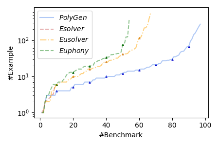
(a) Results of Exp1 for $\mathbb{O}_{V}$ of example

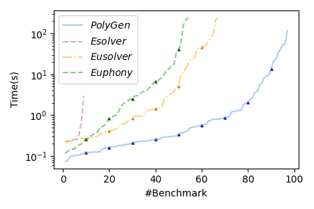
(b) Results of Exp1 for $\mathbb{O}_{V}$ of time

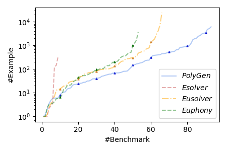
(c) Results of Exp1 for $\mathbb{O}_{R}$ of example

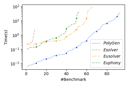
(d) Results of Exp1 for $\mathbb{O}_{R}$ of time

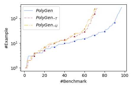
(e) Results of Exp2 for $\mathbb{O}_{V}$ of example

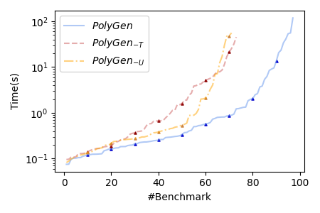
(f) Results of Exp2 for $\mathbb{O}_{V}$ of time

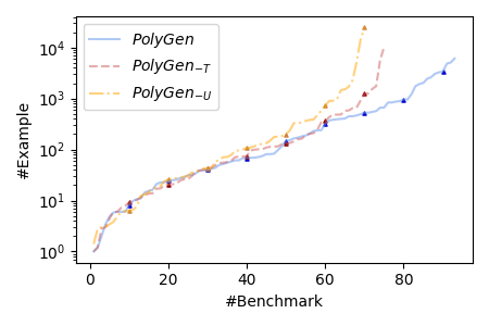
(g) Results of Exp2 for $\mathbb{O}_{R}$ of example

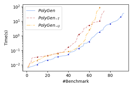
(h) Results of Exp2 for $\mathbb{O}_{R}$ of time

Figure 2. The results of exp1 and exp2. For each approach, we sort its solved benchmarks in the increasing order of the time cost or number of examples needed. Scatters are added for every 10 benchmarks.

Comparing with Eusolver and Euphony, PolyGen performs significantly better on both generalizability and efficiency. The expreimental result on the generalizability is consistent with our theoretical analysis, as PolyGen is an Occam solver but Eusolver, Euphony are not. Comparing with $\mathbb{O}_{V}$, the advantage of PolyGen on oracle model $\mathbb{O}_{R}$ seems less attractive. The reason is that on $\mathbb{O}_{R}$, the cost of distinguishing an incorrect program increases, and thus the effect of synthesis algorithms is weakened. For example, in benchmark qm_neg_1.sl, it is hard to distinguish between the target program is $p^{*}(x)=(\texttt{if}\ (x<0)\ \texttt{then}\ 1\ \texttt{else}\ 0)$ and a wrong program with a slightly different if-condition $p^{\prime}(x)=(\texttt{if}\ (x\leq 0)\ \texttt{then}\ 1\ \texttt{else}\ 0)$ in model $\mathbb{O}_{R}$, as the probability for a random input to distinguish them is smaller than $1\%$ when the input is in the range $[-50,50]$.

Please note that the comparison in Column #Example suffers from a survivorship bias: On a large number of cases that PolyGen solves while Eusolver or Euphony does not, PolyGen is likely to have better generalizability. To validate this point, we perform an extra experiment on model $\mathbb{O}_{R}$. We iteratively rerun Eusolver and Euphony on those benchmarks where PolyGen solves but Eusolver or Euphony does not. Starting from only $1$ random example, we invoke Eusolver or Euphony with an enlarged time-limit of 30 minutes. If the solver synthesizes an incorrect program, we record the current number of examples as a lower bound of the generalizability, and then continue to the next iteration by doubling the number of examples. The iteration stops when Eusolver or Euphony successfully synthesizes a correct program or times out. After adding these lower bounds, the geometric mean of the ratios between the lower bounds and the number of examples used by PolyGen is reported in column #Example$\leq$ of Table 2. The result justifies the existence of the survivorship bias as the ratios increase from $\times 1.115-\times 1.649$ to $\times 3.320-\times 3.302$. Please note that the new experiment still favors to Eusolver and Euphony because (1) the iteration only provides a coarse lower bound on the number of required examples, (2) the survivorship bias still exists as Eusolver and Euphony still time out on 27 and 28 out of 93 benchmarks, respectively.

In terms of efficiency, PolyGen solves almost all benchmarks in $\mathcal{D}$ on both oracle models. We investigate those benchmarks where PolyGen times out, and conclude two major reasons:

• As the time cost of $\mathcal{T}_{\text{poly}}$ grows quickly when the number of if-terms increases, PolyGen may time out when a large term set is used. For example, PolyGen fails in finding a valid term set for array_serach_15.sl as this benchmark requires $16$ different if-terms.

• As $\mathcal{U}_{\text{poly}}$ consider conditions in the increasing order of the size, PolyGen may time out when a large condition is used. For example, PolyGen times out on mpg_example3.sl which uses if-condition $2x+2y-z-7\leq 0$. This defect can be improved by combining PolyGen with techniques on feature synthesis (Padhi and Millstein, 2017).

At last, a noteworthy result is that Euphony performs even worse than Eusolver in our evaluation, implying that the model used in Euphony plays a negative role. One possible reason is that the target programs in our dataset are diverse and are not easily predictable with a simple probabilistic model considering only the dependency between program elements.

9.3. Exp2: Comparison of the Term Solver and the Unifier (RQ2)

Procedure. In this experiment, we test how $\mathcal{T}_{\text{poly}}$ and $\mathcal{U}_{\text{poly}}$ affect the performance of PolyGen.

Here, we implement two weakened solvers $\textit{PolyGen}_{-T}$ and $\textit{PolyGen}_{-U}$: $\textit{PolyGen}_{-T}$ replaces term solver $\mathcal{T}_{\text{poly}}$ with the term solver $\mathcal{T}_{E}$ used in Eusolver, and $\textit{PolyGen}_{-U}$ replaces unifier $\mathcal{U}_{\text{poly}}$ with the unifier $\mathcal{U}_{E}$ used in Eusolver. For each oracle model, we run these solvers on all benchmarks in $\mathcal{D}$.

Results. The results are summarized in Table 3 while more details are drawn as Figure 2.

Table 3. The results of comparing PolyGen with weakened solvers.

Model	$\mathbb{O}_{V}$			$\mathbb{O}_{R}$
Solver	#Solved	#Example	Time Cost	#Solved	#Example	Time Cost
PolyGen	$97$	$\times 1.000$	$\times 1.000$	$93$	$\times 1.000$	$\times 1.000$
$\textit{PolyGen}_{-T}$	$73$	$\times 1.154$	$\times 2.001$	$75$	$\times 0.956$	$\times 2.728$
$\textit{PolyGen}_{-U}$	$71$	$\times 1.644$	$\times 1.95$	$70$	$\times 1.307$	$\times 1.943$

As shown in Table 3, the unifier $\mathcal{U}_{\text{poly}}$ improves a lot on both efficiency and generalizability. In contrast, $\mathcal{T}_{\text{poly}}$ majorly contributes to the efficiency, as the generalizability of PolyGen changes little when $\mathcal{T}_{\text{poly}}$ is replaced. The reason is that the number of examples required by the unifier usually dominates the number of examples required by the term solver, because an example for synthesizing if-conditions, where the output type is Boolean, provides much less information than an example for synthesizing if-terms, where the output is an integer.

10. Conclusion

In this paper, we adopt a concept from computational learning theory, Occam Learning, to study the generalizability of the STUN framework. On the theoretical side, we provide a sufficient set of conditions for individual components in STUN to form an Occam solver and prove that Eusolver, a state-of-the-art STUN solver, is not an Occam solver. Besides, we design an Occam solver PolyGen for the STUN framework. On the practical side, we instantiate PolyGen on the domains of CLIA and evaluate it against state-of-the-art PBE solvers on 100 benchmarks and 2 common oracle models. The evaluation shows that (1) PolyGen significantly outperforms existing STUN solvers on both efficiency and generalizability, and (2) PolyGen keeps almost the same generalizability with those solvers that always synthesize the smallest program, but achieves significantly better efficiency.

Appendix A Appendix: Occam Learning

In this section, we compare the difference between the original definition of Occam Learning provided by Blumer et al. (1987) and the extended definition used in this paper (Definition 4.2).

Definition A.1 (Original Definition of Occam Learning).

Let $\mathbb{C},\mathbb{H}$ be the concept classes containing target concepts and hypotheses respectively. Then, for constants $\alpha\geq 0$ and $0\leq\beta<1$, a learning algorithm $\mathcal{L}$ is an $(\alpha,\beta)$-Occam algorithm for $\mathbb{C}$ using $\mathbb{H}$ iff, given a set $S=\{x_{1},\dots,x_{m}\}$ of $m$ samples labeled according to a concept $c\in\mathcal{\mathbb{missing}}C$, $\mathcal{L}$ outputs a hypothesis $h\in\mathbb{H}$ such that:

• $h$ is consistent with $c$ on $S$, i.e., $\forall x\in S,h(x)=c(x)$.

• $\text{size}(h)\leq(N\cdot\text{size}(c))^{\alpha}m^{\beta}$.

where $N$ is the maximum length of any sample $x\in S$, $\text{size}(c)$ and $\text{size}(h)$ are the lengths of the binary representations of concept $c$ and hypothesis $h$ respectively.

Definition A.2 (Definition 4.2).

For constants $\alpha\geq 1,0\leq\beta<1$, PBE solver $\mathcal{S}$ is an $(\alpha,\beta)$-Occam solver on a family of domains $\mathcal{F}$ if there exist constants $c,\gamma>0$ such that for any program domain $\mathbb{D}\in\mathcal{F}$, for any target program $p^{*}\in\mathbb{P}$, for any input set $\{I_{1},\dots,I_{n}\}\subseteq\mathbb{I}$, for any error rate $\epsilon\in\left(0,\frac{1}{2}\right)$:

$$\Pr\left[\text{size}\left(\mathcal{S}\big{(}T(p^{*},I_{1},\dots,I_{n})\big{)}\right)>c\left(\text{size}(p^{*})\right)^{\alpha}n^{\beta}\ln^{\gamma}\left(\frac{1}{\epsilon}\right)\right]\leq\epsilon$$

where size$(p)$ is the length of the binary representation of program $p$, $T(p,I_{1},\dots,I_{n})$ is defined as the PBE task corresponding to target program $p^{*}$ and inputs $I_{1},\dots,I_{n}$.

To adopt the concept Occam Learning to our paper, we firstly replace terms in Definition A.1 with their counterparts in programming by example:

• The classes of concepts $\mathbb{C}$ and hypotheses $\mathbb{H}$ both correspond to the program space $\mathbb{P}$.

• The learner $\mathcal{L}$ corresponds to a PBE solver $\mathcal{S}$.

• The target concept $c$, samples $S=\{x_{1},\dots,x_{m}\}$, the set of labeled samples and the learned hypothesis $h$ correspond to the target program $p^{*}$, the set of inputs $\{I_{1},\dots,I_{n}\}$, the PBE task $T(p^{*},I_{1},\dots,I_{n})$ and the synthesized program $\mathcal{S}(T(p^{*},I_{1},\dots,I_{n}))$ respectively.

Second, for simplicity, we assume that the range of an input variable is finite and bounded, and thus ignore the cost of expressing samples, i.e., variable $N$ in Definition A.1. When the range of an input variable is bounded, a sample can be expressed using $O(k)$ bits, where $k$ is the number of input variables, and thus $N$ can be bounded by $O(\text{size}(p^{*}))$. Therefore, at this time, removing $N$ from the upper bound would not affect the class of Occam algorithms (solvers), though the concrete values of constants $\alpha$ and $\beta$ may be changed.

Third, we extend Definition A.1 to support randomness by introduing error rate $\epsilon$. In Definition A.2, a random PBE solver $\mathcal{S}$ is allowed to returned a program larger than the upper bound, but the probability should be bounded. In Definition A.2, factor $\ln(1/\epsilon)$ is introduced to limit the size of the returned programs concentrate to the original polynomial bound, and thus we could prove a theoretical guarantee on the generalizability of a random Occam solver that is similar with the guarantee for deterministic Occam solvers.

Theorem A.3 (Theorem 4.6).

Let $\mathcal{S}$ be an $(\alpha,\beta)$-Occam solver on domain $\mathbb{D}$. Then there exist constants $c,\gamma>0$ such that for any $0<\epsilon,\delta<1$, for any distribution $D$ over $\mathbb{I}$ and for any target program $p^{*}\in\mathbb{P}$:

$$\small\forall n>c\left(\frac{1}{\epsilon}\ln\left(\frac{2}{\delta}\right)+\left(\frac{(\text{size}(p^{*}))^{\alpha}\ln^{\gamma}(2/\delta)}{\epsilon}\right)^{1/(1-\beta)}\right),\Pr_{I_{i}\sim D}\left[\text{err}_{D,p^{*}}\left(\mathcal{S}\big{(}T(p^{*},I_{1},\dots,I_{n})\big{)}\right)\geq\epsilon\right]\leq\delta$$

where $\text{err}_{D,p^{*}}(p)$ represents the error rate of program $p$ when the input distribution is $D$ and the target program is $p^{*}$, i.e., $\text{err}_{D,p^{*}}(p)\coloneqq\Pr_{I\sim D}\left[\llbracket{p}\rrbracket(I)\neq\llbracket{p^{*}}\rrbracket(I)\right]$.

Proof.

By Definition A.2, there exists constants $c^{\prime},\gamma^{\prime}$ such that:

(2) $$\Pr\left[\text{size}\left(\mathcal{S}\big{(}T(p^{*},I_{1},\dots,I_{n})\big{)}\right)>c^{\prime}\left(\text{size}(p^{*})\right)^{\alpha}n^{\beta}\ln^{\gamma^{\prime}}\left(\frac{2}{\delta}\right)\right]\leq\frac{\delta}{2}$$

Let $\mathbb{P}_{\delta}$ be the set of programs sastisfying that the size is no larger than $c^{\prime}\left(\text{size}(p^{*})^{\alpha}n^{\beta}\ln^{\gamma}(2/\delta)\right)$. By Lemma 4.5, we have an upper bound on $|\mathbb{P}_{\delta}|$:

$$\ln|\mathbb{P}_{\delta}|\leq c^{\prime}(\ln 2)\left(\text{size}(p^{*})^{\alpha}n^{\beta}\ln^{\gamma^{\prime}}(2/\delta)\right)$$

Let $\mathcal{E}$ be the event where $\mathcal{S}$ returns a program outside $\mathbb{P}_{\delta}$. Then by Equation 2, $\Pr[\mathcal{E}]\leq\frac{\delta}{2}$. Besides, let $\mathbb{P}_{\epsilon,\delta}\subseteq\mathbb{P}_{\delta}$ be the set of program $p$ in $\mathbb{P}_{\delta}$ satisfying $\textit{err}_{D,p^{*}}(p)\geq\epsilon$. Then:

$$\Pr_{I_{i}\sim D}\left[\textit{err}_{D,p^{*}}\left(\mathcal{S}\big{(}T(p^{*},I_{1},\dots,I_{n})\big{)}\right)\geq\epsilon\right] \leq\Pr_{I_{i}\sim D}[\mathcal{E}]+\Pr_{I_{i}\sim D}\left[\forall p\in\mathbb{P}_{\epsilon,\delta},\big{(}\exists I\in[1,n],\llbracket{p}\rrbracket(I)\neq\llbracket{p^{\prime}}\rrbracket(I)\big{)}\right]$$

$$\leq\frac{\delta}{2}+|\mathbb{P}_{\delta}|(1-\epsilon)^{n}$$

Therefore, we obtain the following inequality on $n$:

$$\Pr_{I_{i}\sim D}\left[\textit{err}_{D,p^{*}}\left(\mathcal{S}\big{(}T(p^{*},I_{1},\dots,I_{n})\big{)}\right)\geq\epsilon\right]\leq\delta$$

$$\Longleftarrow \ |\mathbb{P}_{\delta}|(1-\epsilon)^{n}\leq\frac{\delta}{2}$$

$$\Longleftarrow \ n\ln\left(\frac{1}{1-\epsilon}\right)n\geq\ln\left(\frac{2}{\delta}\right)+c^{\prime}(\ln 2)\left(\text{size}(p^{*})^{\alpha}n^{\beta}\ln^{\gamma^{\prime}}\left(\frac{2}{\delta}\right)\right)$$

$$\Longleftarrow \ n\geq\frac{1}{\epsilon}\ln\left(\frac{2}{\delta}\right)+\frac{c^{\prime}(\ln 2)}{\epsilon}\left(\text{size}(p^{*})^{\alpha}n^{\beta}\ln^{\gamma^{\prime}}\left(\frac{2}{\delta}\right)\right)$$

$$\Longleftarrow \ n\geq c\left(\frac{1}{\epsilon}\ln\left(\frac{2}{\delta}\right)+\left(\frac{(\text{size}(p^{*}))^{\alpha}\ln^{\gamma}(2/\delta)}{\epsilon}\right)^{1/(1-\beta)}\right)$$

where $c$ is a large enough constant and $\gamma=\gamma^{\prime}$. ∎

Appendix B Appendix: Proofs

In this section, we complete the proofs of the theorems in our paper.

Lemma B.1 (Lemma 4.5).

For any domain $\mathbb{D}$, $\forall p\in\mathbb{P}$, $\left|\left\{p^{\prime}\in\mathbb{P}\ |\ \text{size}(p^{\prime})\leq\text{size}(p)\right\}\right|\leq 2^{\text{size}(p)}$.

Proof.

Let $n$ be the number of grammar rules used to derive program $p$, $R$ be the set of available grammar rules, and $N$ be the size of $R$. Let $r^{*}$ be an arbitrary rule in $R$.

Let $\mathbb{P}_{p}$ be the set of all program $p^{\prime}$ satisfying $\text{size}(p^{\prime})\leq\text{size}(p)$. Define function $\varphi:\mathbb{P}_{p}\mapsto R^{n}$ as $\varphi(p)\coloneqq r_{1}\dots r_{n^{\prime}}r^{*}\dots r^{*}$, where $r_{1}\dots r_{n^{\prime}}$ is the leftmost derivation of program p’, and $r^{*}$ repeats for $n-n^{\prime}$ times. Clearly, $\varphi$ is an injection, i.e., $\forall p_{1},p_{2}\in\mathbb{P}_{p},p_{1}\neq p_{2}\implies\varphi(p_{1})\neq\varphi(p_{2})$.

Therefore, $|\mathbb{P}_{p}|\leq|R^{n}|\leq N^{n}\leq 2^{\text{size}(p)}$. ∎

Theorem B.2 (Theorem 4.7).

Let $\mathcal{F}^{A}$ be the family of all possible domains. Then $\mathcal{S}_{\text{min}}$ is an $(1,0)$-Occam solver on $\mathcal{F}^{A}$, and $\mathcal{S}_{\text{rand}}$ is not an Occam solver on $\mathcal{F}^{A}$.

Proof.

We start with $\mathcal{S}_{\text{min}}$. Let $p^{*}$ be the target program and $p$ be the program synthesized by $\mathcal{S}_{\text{min}}$. By the definition of $\mathcal{S}_{\text{min}}$, $\text{size}(p)\leq\text{size}(p^{*})$. Therefore, $\mathcal{S}_{\text{min}}$ is an $(1,0)$-Occam solver.

For $\mathcal{S}_{\text{rand}}$, suppose that all programs in the program space satisfy all given examples, and the target program $p^{*}$ is the smallest program in the program space. Let $p$ be the program synthesized by $\mathcal{S}_{\text{rand}}$. Then, by the definition of $\mathcal{S}_{\text{rand}}$, $p$ follows a uniform distribution on the program space. Therefore, $\text{size}(p)$ can be arbitrarily larger than $\text{size}(p^{*})$, and $\mathcal{S}_{\text{rand}}$ is not an Occam solver. ∎

Theorem B.3 (Theorem 5.7).

Let $\mathcal{F}_{C}$ be a family of if-closed conditional domains, $\mathcal{T}$ be an $(\alpha_{1},\beta_{1})$-Occam term solver on $\mathcal{F}_{C}$, $\mathcal{U}$ be an $(\alpha_{2},\beta_{2})$-Occam unifier where $\beta_{1}\alpha_{2}+\beta_{2}<1$. Then the STUN solver comprised of $\mathcal{T}$ and $\mathcal{U}$ is an $((\alpha_{1}+1)\alpha_{2},\beta_{1}\alpha_{2}+\beta_{2})$-Occam solver.

Proof.

Let $p^{*}$ be the target program, and $P=\{t_{1},\dots,t_{n}\}$ be the term set synthesized by $\mathcal{T}$. By the definition of an Occam term solver, there exists constants $c_{1}$ and $\gamma_{1}$ such that:

$$\forall\epsilon_{1}\in\left(0,\frac{1}{2}\right),\Pr\left[\text{tsize}\left(P\right)>c_{1}\left(\text{size}(p^{*})\right)^{\alpha_{1}}n^{\beta_{1}}\ln^{\gamma_{1}}\left(\frac{1}{\epsilon_{1}}\right)\right]\leq\epsilon_{1}$$

We construct the following function $\varphi:\mathbb{P}_{t}\mapsto(P,\mathbb{P}_{c})$ that converts a term into the program space of the unifier $\mathcal{U}$:

$$\varphi(t)\coloneqq\texttt{if }(t=t_{1})\texttt{ then }t_{1}\texttt{ else }\dots\texttt{ else if }(t=t_{n-1})\texttt{ then }t_{n-1}\texttt{ else }t_{n}$$

By the definition of $\text{size}(p)$, $\text{size}(\varphi(t))\leq 2\lceil\log_{2}N\rceil+n\cdot\text{size}(t)+2\text{tsize}(P)\leq c_{3}\text{size}(t)\text{tsize}(P)$, where $N$ is the number of grammar rules, $c_{3}$ is a large enough constant.

$\varphi$ can be extend to the whole program space $(\mathbb{P}_{t},\mathbb{P}_{c})$ where $\varphi(p)$ is the program replacing all terms $t$ used in $p$ with $\varphi(t)$. Clearly, $\text{size}(\varphi(p))$ is no larger than $c_{3}\text{size}(p)\text{tsize}(P)$.

Let $p_{u}$ be the program synthesized by $\mathcal{U}$. As $\varphi(p^{*})$ is a valid program for the unifier $\mathcal{U}$, by the definition of an Occam unifier, there exists constants $c_{2}$ and $\gamma_{2}$ such that:

$$\forall\epsilon_{2}\in\left(0,\frac{1}{2}\right),\Pr\left[\text{size}\left(p_{u}\right)>c_{2}\big{(}\max(\text{size}(\varphi(p^{*})),\text{tsize}(P))\big{)}^{\alpha_{2}}n^{\beta_{2}}\ln^{\gamma_{2}}\left(\frac{1}{\epsilon_{2}}\right)\right]\leq\epsilon_{2}$$

For any $\epsilon\in\left(0,\frac{1}{2}\right)$, by taking $\epsilon_{1}=\epsilon_{2}=\frac{1}{2}\epsilon$, we obtain the following inequality:

$$\Pr\left[\text{tsize}\left(P\right)>c_{1}\left(\text{size}(p^{*})\right)^{\alpha_{1}}n^{\beta_{1}}\ln^{\gamma_{1}}\left(\frac{2}{\epsilon}\right)\right]\leq\frac{\epsilon}{2}\bigwedge$$

$$\Pr\left[\text{size}\left(p_{u}\right)>c_{2}\big{(}\max(\text{size}(\varphi(p^{*})),\text{tsize}(P))\big{)}^{\alpha_{2}}n^{\beta_{2}}\ln^{\gamma_{2}}\left(\frac{2}{\epsilon}\right)\right]\leq\frac{\epsilon}{2}$$

$$\implies \Pr\left[\text{size}\left(p_{u}\right)>c_{2}\left(c_{1}c_{3}\left(\text{size}(p^{*})\right)^{\alpha_{1}+1}n^{\beta_{1}}\ln^{\gamma_{1}}\left(\frac{2}{\epsilon}\right)\right)^{\alpha_{2}}n^{\beta_{2}}\ln^{\gamma_{2}}\left(\frac{2}{\epsilon}\right)\right]\leq\epsilon$$

$$\implies \Pr\left[\text{size}\left(p_{u}\right)>c\left(\text{size}(p^{*})\right)^{(\alpha_{1}+1)\alpha_{2}}n^{\beta_{1}\alpha_{2}+\beta_{2}}\ln^{\gamma}\left(\frac{1}{\epsilon}\right)\right]\leq\epsilon$$

where $c$ is a large enough constant and $\gamma=\gamma_{1}\alpha_{2}+\gamma_{2}$.

Therefore, the STUN solver comprised of $\mathcal{T}$ and $\mathcal{U}$ is an $((\alpha_{1}+1)\alpha_{2},\beta_{1}\alpha_{2}+\beta_{2})$-Occam solver. ∎

Theorem B.4 (Theorem 5.9).

$\mathcal{T}_{E}$ is not an Occam term solver on $\mathcal{F}^{A}_{C}$, and Eusolver is not an Occam solver on $\mathcal{F}^{A}_{C}$, where $\mathcal{F}^{A}_{C}$ is the family of all if-closed conditional domains.

Proof.

This theorem is directly from Example 5.8. ∎

Theorem B.5 (Theorem 5.10).

There is no polynomial-time Occam unifier on $\mathcal{F}^{A}_{C}$ unless $\mathsf{NP}=\mathsf{RP}$.

Proof.

Suppose there is a polynomial-time Occam unifier $\mathcal{U}$. Given a decision tree learning problem with $k$ different tests and $n$ data $d_{1},\dots,d_{n}$ labeled with $m$ different labels. We construct a conditional program domain $\mathbb{D}$ where:

• Input space $\mathbb{I}$ contains $n$ different inputs, corresponding to data $d_{1},\dots,d_{n}$.

• Term space $\mathbb{P}_{t}$ contains $m$ different constants $1,2,\dots,m$, corresponding to $m$ different labels.

• Condition space $\mathbb{P}_{c}$ contains $k+1$ different conditions $\texttt{false},c_{1},\dots,c_{k}$, where $c_{1},\dots,c_{k}$ correspond to $k$ different tests. If the test result of the $i$th test on data $d_{j}$ is true, $\llbracket{c_{i}}\rrbracket(d_{j})$ will be defined as true. Otherwise, $\llbracket{c_{i}}\rrbracket(d_{j})$ will be defined as false.

Because $\forall a,b\in\mathbb{P}_{t},\forall d_{i}\in\mathbb{I},\llbracket{\texttt{false}}\rrbracket(d_{i})\iff\llbracket{a}\rrbracket(d_{i})=\llbracket{b}\rrbracket(d_{i})$, $\mathbb{D}$ is an if-closed domain.

Let $T=\{(d_{i},l_{i})\}$ be a PBE task where $l_{i}$ is the index of the label corresponding to data $d_{i}$, and let $p$ be the program synthesized by $\mathcal{U}$ for PBE task $T$ and term set $\{1,2,\dots,m\}$. We remove the usages of condition false in $p$ by replacing program ($\texttt{if (false) then }p_{1}\texttt{ else }p_{2}$) with its else-branch $p_{2}$. Suppose $p^{\prime}$ be the resulting program. Clearly, the size of $p^{\prime}$ is no larger than $p$ and $p^{\prime}$ can be mapped back into a decision tree.

So far, we construct a polynomial-time learning algorithm for decision trees based on $\mathcal{U}$. By Theorem 4.6, this construction implies that the class of decision trees is PAC learnable. Combining with the fact that the class of decision trees is not PAC learnable unless $\mathsf{NP}=\mathsf{RP}$ (Hancock et al., 1995), we know there is no polynomial-time Occam unifier unless $\mathsf{NP}=\mathsf{RP}$. ∎

Lemma B.6 (Lemma 6.1).

For constants $\alpha_{1},\alpha_{2}\geq 0,0\leq\beta_{1},\beta_{2}<1$ where $\beta_{1}+\beta_{2}<1$, term solver $\mathcal{T}$ is an $(\alpha_{1}+\alpha_{2},\beta_{1}+\beta_{2})$-Occam solver on $\mathcal{F}_{C}$ if there exist constants $c,\gamma>0$ such that for any conditional domain $\mathbb{D}\in\mathcal{F}_{C}$, any target program $p^{*}\in\mathbb{P}$, and any input set $\{I_{1},\dots,I_{n}\}\subseteq\mathbb{I}$:

1. With a high probability, the size of terms returned by $\mathcal{T}$ is bounded by $\text{size}(p^{*})^{\alpha_{1}}n^{\beta_{1}}$.

   $$\Pr\left[\max\left\{\text{size(p)}\ \big{|}\ p\in\mathcal{T}\big{(}(I_{1},\llbracket{p}\rrbracket(I_{1})),\dots,(I_{n},\llbracket{p}\rrbracket(I_{n}))\big{)}\right\}>c\left(\text{size}(p^{*})\right)^{\alpha_{1}}n^{\beta_{1}}\ln^{\gamma}\left(\frac{1}{\epsilon}\right)\right]\leq\epsilon$$

2. With a high probability, the number of terms returned by $\mathcal{T}$ is bounded by $\text{size}(p^{*})^{\alpha_{2}}n^{\beta_{2}}$.

   $$\Pr\left[\left|\mathcal{T}\big{(}(I_{1},\llbracket{p}\rrbracket(I_{1})),\dots,(I_{n},\llbracket{p}\rrbracket(I_{n}))\big{)}\right|>c\left(\text{size}(p^{*})\right)^{\alpha_{2}}n^{\beta_{2}}\ln^{\gamma}\left(\frac{1}{\epsilon}\right)\right]\leq\epsilon$$

Proof.

Let $P$ be the synthesized term set. For any $\epsilon\in\left(0,\frac{1}{2}\right)$, with a probability of at least $1-\epsilon$:

$$\max\left\{\text{size(p)}\ \big{|}\ p\in\mathcal{P}\right\}\leq c\left(\text{size}(p^{*})\right)^{\alpha_{1}}n^{\beta_{1}}\ln^{\gamma}\left(\frac{2}{\epsilon}\right)\bigwedge\left|P\right|\leq c\left(\text{size}(p^{*})\right)^{\alpha_{2}}n^{\beta_{2}}\ln^{\gamma}\left(\frac{2}{\epsilon}\right)$$

Because $\text{tsize}(P)\leq|P|\cdot\max\left\{\text{size}(p)\ |\ p\in P\right\}$, with a probability of at least $1-\epsilon$:

$$\text{tsize}(P) \leq\left(c\left(\text{size}(p^{*})\right)^{\alpha_{1}}n^{\beta_{1}}\ln^{\gamma}\left(\frac{2}{\epsilon}\right)\right)\cdot\left(c\left(\text{size}(p^{*})\right)^{\alpha_{2}}n^{\beta_{2}}\ln^{\gamma}\left(\frac{2}{\epsilon}\right)\right)$$

$$\leq c^{\prime}\left(\text{size}(p^{*})\right)^{\alpha_{1}+\alpha_{2}}n^{\beta_{1}+\beta_{2}}\ln^{2\gamma}\left(\frac{1}{\epsilon}\right)$$

where $c^{\prime}$ is a large enough constant. Therefore, $\mathcal{T}$ is a $(\alpha_{1}+\alpha_{2},\beta_{1}+\beta_{2})$-Occam solver. ∎

Lemma B.7 (Lemma 6.2).

Let $T$ be a PBE task, and let $P$ be a set of terms that covers all examples in $T$, i.e., $\forall(I,O)\in T,\exists p\in P,\left(\llbracket{p}\rrbracket(I)=O\right)$. There is always a term $p\in P$ such that:

$$\left|\big{\{}(I,O)\in T\ \big{|}\ \llbracket{p}\rrbracket(I)=O\big{\}}\right|\geq|T|/|P|$$

Proof.

Let $t_{1},\dots,t_{n}$ be the terms in $P$, and $w_{1},\dots,w_{n}$ be the number of examples covered by term $t_{i}$, i.e., $w_{i}\coloneqq\left|\left\{(I,O)\in T\ |\ \llbracket{t_{i}}\rrbracket(I)=O\right\}\right|$. As $P$ covers all examples in $T$, $\sum_{i=1}^{n}w_{i}$ must be at least $|T|$. Therefore, we have $\max w_{i}\geq|T|/|P|$. ∎

Theorem B.8 (Theorem 6.3).

$\mathcal{S}_{t}$ is an $(\alpha,\beta)$-Occam solver on $T(\mathcal{F}_{C})\implies\mathcal{T}_{\text{poly}}$ is an $(\alpha^{\prime}+1,\beta^{\prime})$-Occam term solver on $\mathcal{F}_{C}$ for any $\alpha^{\prime}>\alpha,\beta<\beta^{\prime}<1$, where $T(\mathcal{F}_{C})$ is defined as $\{(\mathbb{P}_{t},\mathbb{I}^{\prime})\ |\ ((\mathbb{P}_{t},\mathbb{P}_{c}),\mathbb{I})\in\mathcal{F}_{C},\mathbb{I}^{\prime}\subseteq\mathbb{I}\}$.

Proof.

Let $s^{*}$ be the value of variable $s$ (Line 19 in Algorithm 1) when $\mathcal{T}_{\text{poly}}$ terminates. Let $p^{*}$ be the target program, $P^{*}$ be the terms used by $\mathcal{T}_{\text{poly}}$, $P$ be the term set synthesized by $\mathcal{T}_{\text{poly}}$, and $n$ be the number of examples, i.e., $|T|$. By Algorithm 1, the total size of $P$ is bounded by $s^{*}$:

$$\text{tsize}(P)\leq|P|\cdot\max_{p\in P}\text{size}(p)\leq cs^{*}\log n\cdot c(s^{*})^{\alpha}n^{\beta}\leq c^{\prime}(s^{*})^{\alpha+1}n^{\beta^{\prime\prime}}$$

where $\beta^{\prime\prime}$ is a constant larger than $\beta$ and $c^{\prime}$ is a large enough constant.

Let $c_{1}$ be a large enough constant, $\alpha^{\prime}$ be any constant larger than $1$, $\beta^{\prime}$ be any constant larger than $0$. Suppose $s\geq c_{1}\text{size}(p^{*})^{\alpha^{\prime}}n^{\beta^{\prime}}$, $n_{t}=cs^{\alpha/(1-\beta)}$, $k_{t}=cs\log n$. We denote an invocation Search($T^{\prime},k,n_{t},s$) valid if the following three random events happens:

• $\mathcal{E}_{1}$: There is at least one valid sampling round, where a sampling round is valid if $t^{*}$ covers all sampled examples, and $t^{*}$ is the target term in $P^{*}$ that covers the most examples in $T^{\prime}$.

• $\mathcal{E}_{2}$: $\text{size}(t_{0})\leq cs^{\alpha}n_{t}^{\beta}$, where $t_{0}$ is the term synthesized in the first valid sampling round.

• $\mathcal{E}_{3}$: $\text{size}(t_{0})$ covers at least a half of those examples covered by $t^{*}$ in $T^{\prime}$, i.e.,

  $$\left(\big{|}\textnormal{{Covered(}}\textnormal{\emph{$t_{0},T^{\prime}$}}\textnormal{{)}}\cap\textnormal{{Covered(}}\textnormal{\emph{$t^{*},T^{\prime}$}}\textnormal{{)}}\big{|}\geq\frac{1}{2}\big{|}\textnormal{{Covered(}}\textnormal{\emph{$t^{*},T^{\prime}$}}\textnormal{{)}}\big{|}\right)\wedge\left(\big{|}\textnormal{{Covered(}}\textnormal{\emph{$t^{*},T^{\prime}$}}\textnormal{{)}}\big{|}>0\right)$$

Consider a recursion chain $RC$ of function Search() with examples $T^{\prime}_{0}=T,\dots,T^{\prime}_{n_{c}}=\emptyset$, where $T_{i}$ recurses into $T_{i+1}$ by including $t_{0}$ in the result, i.e., $T_{i+1}=T_{i}-\textnormal{{Covered(}}\textnormal{\emph{$p^{*},T_{i}$}}\textnormal{{)}}$.

• Claim: When all these invocations are valid, $n_{c}$ is at most $2|P^{*}|\ln|T|+1$.

• Proof: By the definition of $t^{*}$, $|\textnormal{{Covered(}}\textnormal{\emph{$t^{*},T_{i}$}}\textnormal{{)}}|\geq|T_{i}|/|P^{*}|$. Then by the definition of $\mathcal{E}_{3}$, we have $|T_{i+1}|\leq\left(1-1/(2|P^{*}|)\right)|T_{i}|$. Therefore, $n_{c}\leq 2|P^{*}|\ln|T|+1$.

Because $k_{t}=cs\log n>2|P^{*}|\ln n$, such a recursion chain is allowed. Therefore, we only need to consider the probability for all invocations to be valid:

• $\mathcal{E}_{1}$. As $t^{*}$ is the target term that covers the most examples, the probability for a random example to be in Covered($t^{*}$, T’) is at least $1/|P^{*}|$. Therefore, the probability for a sampling round to be valid is $|P^{*}|^{-n_{t}}$:

  $$\Pr[\neg\mathcal{E}_{1}]\leq\left(1-|P^{*}|^{-n_{t}}\right)^{n_{t}k^{n_{t}}}\leq\exp(-n_{t})<\frac{1}{12\text{size}(p^{*})\ln n}$$

  The last two inequalities hold when constant $c_{1}$ is large enough.

• $\mathcal{E}_{2}$. As $\mathcal{S}_{t}$ is an $(\alpha,\beta)$-Occam solver, there exists constants $c_{2},\gamma$ such that:

  $$\forall\epsilon\in\left(0,\frac{1}{2}\right),\Pr\left[\text{size}(t_{0})>c_{2}(\text{size}(p^{*}))^{\alpha}n_{t}^{\beta}\ln^{\gamma}\left(\frac{1}{\epsilon}\right)\right]<\epsilon$$

  Therefore, with a probability at least $1-1/(12\text{size}(p^{*})\ln n))$, we have:

  $$\text{size}(t_{0})\leq c_{2}(\text{size}(p^{*}))^{\alpha}n_{t}^{\beta}\ln^{\gamma}(12\text{size}(p^{*})\ln n)<cs^{\alpha}n_{t}^{\beta}$$

  The last inequality holds when constant $c_{1}$ is large enough.

• $\mathcal{E}_{3}$. Let $\mathbb{I}^{\prime}$ be the input space that contains all inputs in Covered($t^{*},T^{\prime}$), and $D$ be a uniform distribution on $\mathbb{I}^{\prime}$. As $\mathcal{S}_{t}$ is an $(\alpha,\beta)$-Occam solver, by Theorem 4.6, $\mathcal{E}_{3}$ happens with a probability of at least $1-1/(12\text{size}(p^{*})\ln n)$ if the following inequality holds:

  $$n_{t}>c_{3}\left(\frac{1}{2}\ln\big{(}24\text{size}(p^{*})\ln n\big{)}+\left(\frac{(\text{size}(p^{*}))^{\alpha}\ln^{\gamma}\big{(}24\text{size}(p^{*})\ln n\big{)}}{\epsilon}\right)^{1/(1-\beta)}\right)$$

  where $c_{3}$ is a fixed constant. Clearly, when $c_{1}$ is large enough, this inequality always holds.

Let $\mathcal{E}_{i}^{S}$ be the random event that the $i$th invocation in $RC$ is valid, and $\mathcal{E}^{RC}$ be the random event that all events in $RC$ are valid. Then:

$$\Pr\left[\neg\mathcal{E}^{RC}\right] \leq\sum_{i=1}^{n_{c}}\Pr\left[\mathcal{E}^{S}_{i}\right]\leq(2|P^{*}|\ln n+1)\big{(}\Pr[\neg\mathcal{E}_{1}]+\Pr[\neg\mathcal{E}_{2}]+\Pr[\neg\mathcal{E}_{3}]\big{)}$$

$$\leq(2\text{size}(p^{*})\ln n+1)\cdot\frac{1}{4\text{size}(p^{*})\ln n}\leq\frac{3}{4}$$

Therefore, when $s$ is larger than $c_{1}\text{size}(p^{*})^{\alpha^{\prime}}n^{\beta^{\prime}}$, in each iteration, $\mathcal{T}_{\text{poly}}$ returns with a probability at least $\frac{1}{4}$. Therefore, for any $\epsilon\in(0,1)$:

$$\Pr\left[s^{*}\leq c_{1}\text{size}(p^{*})^{\alpha^{\prime}}n^{\beta^{\prime}}+c_{4}\ln\left(\frac{1}{\epsilon}\right)\right]<\epsilon$$

$$\implies \Pr\left[\text{tsize}(P^{*})\leq c_{5}\text{size}(p^{*})^{\alpha^{\prime}(1+\alpha)}n^{\beta^{\prime\prime}+(1+\alpha)\beta^{\prime}}\ln\left(\frac{1}{\epsilon}\right)\right]<\epsilon$$

where $c_{4}$ and $c_{5}$ are large enough constants. Note that $\alpha^{\prime}$ is an arbitrary constant larger than $1$, $\beta^{\prime}$ and $\beta^{\prime\prime}$ are arbitrary constants larger than $0$. Therefore, $\mathcal{T}_{\text{poly}}$ is an $(\alpha^{*},\beta^{*})$-Occam term solver for any $\alpha^{*}>1+\alpha,\beta^{*}>0$. ∎

Lemma B.9 ( Lemma 7.1).

For any conditional domain $\mathbb{D}$ and program $p\in(\mathbb{P}_{t},\mathbb{P}_{c})$, there is a program $p^{\prime}\in(\mathbb{P}_{t},\mathbb{P}_{c})_{\text{DL}}$ s.t. (1) $p^{\prime}$ is semantically equivalent to $p$ on $\mathbb{I}$, and (2) $\textit{size}(p^{\prime})\leq 2\textit{size}(p)^{2}$.

Proof.

Let $P=\{t_{1},\dots,t_{m}\}$ be the set of terms used in $p$. Without loss of generality, assume the structure of $p^{\prime}$ is as the following:

$$\texttt{if}\ (c_{1})\ \texttt{then}\ t_{1}\ \texttt{else}\ \texttt{if}\ (c_{2})\ \texttt{then}\ t_{2}\ \texttt{else}\dots\texttt{if}\ (c_{m-1})\ \texttt{then}\ t_{m-1}\ \texttt{else}\ t_{m}$$

For each if-term in $p$, we define its tree path as a sequence $(c_{1},k_{1}),\dots,(c_{n},k_{n})$, where $c_{i}\in\mathbb{P}_{c}$ represents the if-conditions corresponding to this term from the top down, and $k_{i}\in\{0,1\}$ represents the if-branches taken by this term ($0,1$ represent the then-branch and the else-branch respectively). Let $\varphi$ be a function mapping a path to a condition, which is defined as the following:

$$\varphi((c_{1},k_{1}),\dots,(c_{n},k_{n}))\coloneqq\left(\texttt{and}_{k_{i}=0}\ c_{i}\right)\texttt{ and }\left(\texttt{and}_{k_{i}=1}\ (\texttt{not }c_{i})\right)$$

We construct the condition $c_{i}$ from the original program $p$. Let $X_{i}$ be the set of paths corresponding to all usages of term $t_{i}$. Then we construct the corresponding condition $c_{i}$ as $\texttt{or}_{x\in X}\ \varphi(x)$.

Clearly, $p^{\prime}$ is semantically equivalent to $p$ on the input space $\mathbb{I}$. Besides, $c_{1},\dots,c_{m-1}$ are all DNF formulas, and thus $p^{\prime}\in(\mathbb{P}_{t},\mathbb{P}_{c})_{\text{DL}}$. Let $c_{1}^{\prime},\dots,c_{n_{c}}^{\prime}$ be all if-conditions used in $p$, $l_{i}$ and $r_{i}$ be the numbers of terms used in the then-branch and the else-branch of $c_{i}$ respectively. Then, $\text{size}(p^{\prime})$ can be calculated in the following way:

• The total size of if-conditions $c_{i}$ is at most:

  $$\sum_{i=1}^{n_{c}}\big{(}l_{i}(\text{size}(c^{\prime}_{i})+\lceil\log_{2}N\rceil)+r_{i}(\text{size}(c^{\prime}_{i})+2\lceil\log_{2}N\rceil)\big{)}-(m-1)\lceil\log_{2}N\rceil$$

  where $N$ is the number of grammar rules.

• The total size of if-operators is $(m-1)\lceil\log_{2}N\rceil$, the total size of if-terms is $\sum_{i=1}^{m}\text{size}(t_{i})$.

Therefore, we have the following inequality:

$$\text{size}(p^{\prime})\leq \sum_{i=1}^{n_{c}}\big{(}l_{i}(\text{size}(c^{\prime}_{i})+\lceil\log_{2}N\rceil)+r_{i}(\text{size}(c^{\prime}_{i})+2\lceil\log_{2}N\rceil)\big{)}$$

$$-(m-1)\lceil\log_{2}N\rceil+(m-1)\lceil\log_{2}N\rceil+\sum_{i=1}^{m}\text{size}(t_{i})$$

$$\leq \left(\sum_{i=1}^{n_{c}}(l_{i}+r_{i})\text{size}(c_{i}^{\prime})+\sum_{i=1}^{m}\text{size}(t_{i})\right)+2\lceil\log_{2}N\rceil\sum_{i-1}^{n_{c}}(l_{i}+r_{i})$$

$$\leq \text{size}(p)\left(\sum_{i=1}^{n_{c}}\text{size}(c_{i}^{\prime})+\sum_{i=1}^{m}\text{size}(t_{i})\right)+\text{size}(p)\cdot 2n_{c}\lceil\log_{2}N\rceil\leq 2\text{size}(p)^{2}$$

where $2n_{c}\lceil\log_{2}N\rceil\leq\text{size}(p)$ because each if-condition corresponds to an occurrence of itself and an if-then-else operator: Both of them contributes to $\text{size}(p)$ by at least $\lceil\log_{2}N\rceil$. ∎

Lemma B.10 (Lemma 7.2).

$\mathcal{C}$ is an $(\alpha,\beta)$-Occam solver on $\text{DNF}(\mathcal{F}_{C})\Rightarrow\mathcal{U}_{\text{poly}}$ is an $(\alpha^{\prime},\beta)$-Occam unifier on $\mathcal{F}_{C}$ for any $\alpha^{\prime}>4\alpha$, where $\text{DNF}(\mathcal{F}_{C})$ is defined as $\{(\text{DNF}(\mathbb{P}_{c}),\mathbb{I}^{\prime})\ |\ ((\mathbb{P}_{t},\mathbb{P}_{c}),\mathbb{I})\in\mathcal{F}_{C},\mathbb{I}^{\prime}\subseteq\mathbb{I}\}$.

$\mathcal{C}$ is a deterministic $(\alpha,\beta)$-Occam solver on $\text{DNF}(\mathcal{F}_{C})\Rightarrow\mathcal{U}_{\text{poly}}$ is a $(4\alpha,\beta)$-Occam unifier on $\mathcal{F}_{C}$.

Proof.

Let $P=\{t_{1},\dots,t_{m}\}$ be the term set and $p^{*}\in(P,\mathbb{P}_{c})$ be the target program. Let $c_{1}^{*},\dots,c_{m-1}^{*}$ be the if-conditions for $t_{i}$ in the same way as the proof of Lemma 7.1. Specially, if term $t_{i}$ is not used in $p^{*}$, $t_{i}$ is defined as false. Let $s=\max(\text{tsize}(P),\text{size}(p^{*}))$. By the construction of $c_{i}^{*}$, we have (1) $\sum_{i=1}^{m-1}\text{size}(c_{i}^{*})\leq O(s^{2})$, and (2) $c_{1}^{*},\dots,c_{m-1}^{*}$ never overlap, i.e., $\forall 1<i<j<m,\forall I\in\mathbb{I},\neg(\llbracket{c_{i}^{*}}\rrbracket(I)\wedge\llbracket{c_{j}^{*}}\rrbracket(I))$.

Let $T_{i}$ be the set of examples that are satisfied by term $t_{i}$ and are not satisfied by any term in $t_{i+1},\dots,t_{m}$. By Algorithm 3, the set of positive examples provided to synthesize $c_{i}^{*}$ must be a subset of $T_{i}$. As $c_{i}^{*}$ may not satisfy all positive examples in $T_{i}$, we construct conditions $c^{\prime}_{1},\dots,c^{\prime}_{m-1}$ instead:

$$c^{\prime}_{i}\coloneqq c_{i}^{*}\texttt{ or }\left(\text{or}_{j=1}^{i-1}\ \left(\texttt{or}_{k=1}^{n_{j}}\ \left(c_{j,k}^{*}\texttt{ and }\left(t_{i}=t_{j}\right)\right)\right)\right)$$

where $c_{i,1}^{*},\dots,c_{i,n_{i}}^{*}$ are the clauses used in condition $c_{i}^{*}$, i.e., $c_{i}^{*}=\texttt{or}_{j=1}^{n_{i}}\ c_{i,j}^{*}$. Clearly, $c_{i}^{\prime}$ is still a DNF formula, and $c_{i}^{\prime}$ satisfies all examples in $T_{i}$. Therefore, $c_{i}^{\prime}$ is always a target condition for the PBE task corresponding to $c_{i}$. As in $c^{\prime}_{1},\dots,c^{\prime}_{m-1}$, each clause $c_{i,j}^{*}$ in condition $c_{i}^{*}$ occurs at most $m-1$ times, each time with a comparison $t_{i}=t_{k}$. Therefore, $\sum_{i=1}^{m-1}\text{size}(c_{i}^{\prime})=O(s^{4})$.

Let $c_{1},\dots,c_{m-1}$ be the condition synthesized by $\mathcal{C}$. Let $\epsilon$ be any constant in $\left(0,\frac{1}{2}\right)$. For simplicity, we abbreviate $\text{size}(c_{i}^{\prime})$ as $s_{i}$. When $\mathcal{C}$ is an $(\alpha,\beta)$-Occam solver, there exist constants $c^{\prime},\gamma^{\prime}$ such that:

$$\forall i\in[1,m-1],\Pr\left[\text{size}(c_{i})>c^{\prime}s_{i}^{\alpha}|T|^{\beta}\ln^{\gamma^{\prime}}\left(\frac{m-1}{\epsilon}\right)\right]\leq\frac{\epsilon}{m-1}$$

Therefore, with a probability of at least $1-\epsilon$:

$$\sum_{i=1}^{m-1}\text{size}(c_{i}) \leq c^{\prime}|T|^{\beta}\ln^{\gamma^{\prime}}\left(\frac{m-1}{\epsilon}\right)\sum_{i=1}^{m-1}s_{i}^{\alpha}\leq c^{\prime}|T|^{\beta}\left(\ln(m-1)+\ln\left(\frac{1}{\epsilon}\right)\right)^{\gamma^{\prime}}\left(\sum_{i=1}^{m-1}s_{i}\right)^{\alpha}$$

$$\leq c^{\prime\prime}|T|^{\beta}s^{4\alpha}\ln(m-1)^{\gamma^{\prime}}\ln\left(\frac{1}{\epsilon}\right)^{\gamma^{\prime}}\leq cs^{\alpha^{\prime}}|T|^{\beta}\ln\left(\frac{1}{\epsilon}\right)^{\gamma}$$

where $c^{\prime\prime}$ and $c$ are large enough constants, $\gamma=\gamma^{\prime}$ and $\alpha^{\prime}$ is a constant larger than $4\alpha$. Let $p$ be the program synthesized by $\mathcal{U}_{\text{poly}}$. Then $\text{size}(p)\leq\sum_{i=1}^{m-1}\text{size}(c_{i})+s$. Therefore, when $\mathcal{C}_{\text{CL}}$ is an $(\alpha,\beta)$-Occam solver, $\mathcal{U}_{\text{poly}}$ must be a $(\alpha^{\prime},\beta)$ unifier for any $\alpha^{\prime}>4\alpha$.

When $\mathcal{C}_{\text{CL}}$ is a deterministic $(\alpha,\beta)$-Occam solver, there exists constant $c^{\prime}$ such that:

$$\forall i\in[1,m-1],\text{size}(c_{i})\leq c^{\prime}s_{i}^{\alpha}|T|^{\beta}$$

At this time, we have the following bound on the total size of conditions $c_{1},\dots,c_{m-1}$.

$$\sum_{i=1}^{m-1}\text{size}(c_{i})\leq c^{\prime}s_{i}^{\alpha}|T|^{\beta}\leq c^{\prime}|T|^{\beta}\sum_{i=1}^{m-1}s_{i}^{\alpha}\leq c^{\prime}|T|^{\beta}\left(\sum_{i=1}^{m-1}s_{i}\right)^{\alpha}\leq cs^{4\alpha}|T|^{\beta}$$

where $c$ is a large enough constant. Therefore, at this time, $\mathcal{U}_{\text{poly}}$ is a $(4\alpha,\beta)$-Occam unifier. ∎

Lemma B.11 (Lemma 7.3).

Given condition space $\mathbb{P}_{c}$ and PBE task $T$, let $c^{*}$ be the smallest valid clause and $c$ be the clause found by $\mathcal{C}_{\text{CL}}$. Then $\text{size}(p_{c}(c))<2\text{size}(p_{c}(c^{*}))(\ln|T|+1)$.

Proof.

Let $L$ be the set of available literals, and $L^{*}=\{l_{1},\dots,l_{n}\}$ be the set of literals satisfying all positive examples in $T$. Then, $c$ and $c^{*}$ must be subsets of $L^{*}$.

By Algorithm 3, while applying the greedily algorithm for set covering, we set the cost of a literal as its size. Therefore, by the approximation ratio of this algorithm, we have:

$$\sum_{l\in c}\text{size}(l)<\left(\ln\left|\mathbb{I}_{N}(T)\right|+1\right)\sum_{l\in c^{*}}\text{size}(l)\leq\left(\ln\left|T\right|+1\right)\sum_{l\in c^{*}}\text{size}(l)$$

By this inequality, we have:

$$\text{size}(p_{c}(c)) =\left(|c|-1\right)\lceil\log_{2}N\rceil+\sum_{l\in c}\text{size}(l)<2\sum_{l\in c}\text{size}(l)$$

$$<2\left(\ln\left|T\right|+1\right)\sum_{l\in c^{*}}\text{size}(l)<2\text{size}(p_{c}(c^{*}))(\ln|T|+1)$$

∎

Corollary B.12 (Corollary 7.4).

For any $0<\beta<1$, $\mathcal{C}_{\text{CL}}$ is an $(1,\beta)$-Occam solver on all possible clause domains.

Proof.

For any conditional space $\mathbb{P}_{c}$ and PBE task $T$, let $c^{*}$ be the target clause and $c$ be the clause synthesized by $\mathcal{C}_{\text{CL}}$. By Lemma 7.3, we have:

$$\text{size}(p_{c}(c))<2(\ln|T|+1)\text{size}(p_{c}(c^{*}))<c\text{size}(p_{c}(c^{*}))|T|^{\beta}$$

where $c$ is a large enough constant and $\beta$ is a constant in $(0,1)$. Therefore, for any $0<\beta<1$, $\mathcal{C}_{\text{CL}}$ is an $(1,\beta)$-Occam solver. ∎

Lemma B.13 (Lemma 7.5).

Let $T$ be a PBE task and $d$ be a DNF formula satisfying all examples in $T$:

• All clauses in $d$ must be false on all negative examples in $T$, i.e., $\forall c\in d,\mathbb{I}_{N}(T)\subseteq N(\mathbb{I}(T),c)$.

• There exists a clause in $d$ that is true on at least $|d|^{-1}$ portion of positive examples in $T$, i.e., $\exists c\in d,|P(\mathbb{I}(T),c)|\geq|d|^{-1}|\mathbb{I}_{P}(T)|$.

Proof.

By the semantics of operator or, the first condition is obtained directly. Let $c_{1},\dots,c_{m}$ be the clauses in $d$, and $w_{1},\dots,w_{m}$ be the number of positive examples covered by each clause, i.e., $w_{i}\coloneqq|P(\mathbb{I}(T),c_{i})|$. By the semantics of opeartor or, we know each positive example must be covered by at least one clause. Therefore:

$$w_{1}+\dots+w_{m}\geq|\mathbb{I}_{P}(T)|\implies\max w_{i}\geq m^{-1}|\mathbb{I}_{P}(T)|$$

In this way, the second condition is obtained. ∎

Lemma B.14 (Lemma 7.7).

For any $0<\beta<1$, $\mathcal{C}$ is a $(2,\beta)$-Occam solver on $\text{DNF}(\mathcal{F}_{C}^{A})$.

Proof.

Let $s^{*}$ be the value of variable $s$ (Line 10 in Algorithm 4) when $\mathcal{U}_{\text{poly}}$ terminates. Let $d^{*}$ be the target DNF formula. When $s\geq 2\text{size}(p_{d}(d^{*}))$, $s^{\prime}=s$ and the initial value of $k$ is also $s$, we make the following claim:

• Claim: In invocation Search($\textit{literals},T,k,s$), let $d^{\prime}$ be the set of clauses $c^{*}$ in $d^{*}$ satisfying $P(\mathbb{I}_{P}(T),c^{*})\neq\emptyset$. If $k\geq|d^{\prime}|$, there must be a clause $c\in\textnormal{{Get(}}\textnormal{\emph{$\textit{literals},T,k$}}\textnormal{{)}}$ such that $\exists c^{*}\in d^{\prime},P(\mathbb{I}_{P}(T),c^{*})\subseteq P(\mathbb{I}_{P}(T),c)\wedge\text{size}(p_{c}(c))\leq 2s\ln|T|$.

• Proof: Let $c^{*}$ be the clause in $d^{\prime}$ that covers the most positive examples. Clearly, $|P(\mathbb{I}_{P}(T),c^{*})|\geq|d^{\prime}|^{-1}|\mathbb{I}_{p}(T)|$. As $k\geq d^{\prime}$, the largest clause in $[c^{*}]_{\mathbb{I}_{P}(T)}$ must be in $R(\mathbb{I}_{P}(T),k,\textit{literals})$, and thus this clause is found by Get($\textit{literals},T,k$).

  Let $c$ be the clause simplified from the largest clause in $[c^{*}]_{\mathbb{I}_{P}(T)}$. By Lemma 7.3, $\text{size}(p_{c}(c))<2\text{size}(p_{c}(c^{*}))(\ln|T|+1)\leq 2s\ln|T|$.

By this claim, we obtain that in an iteration where $s>2\text{size}(p_{d}(d^{*}))$, Search() can always find a set of clauses. So, there are at most $O(\text{size}(p_{d}(d^{*})))$ clauses in the DNF formula synthesized by $\mathcal{C}$, and the size of each clause is at most $O(\text{size}(p_{d}(d^{*}))\ln|T|)$. Therefore, the size of the synthesized DNF formula is $O((\text{size}(p_{d}(d^{*})))^{2}\ln|T|)$, which directly implies that $\mathcal{C}$ is a $(2,\beta)$-Occam solver for any $0<\beta<1$.

∎

Theorem B.15 (Theorem 7.8).

For any $0<\beta<1$, $\mathcal{U}_{\text{poly}}$ is a $(8,\beta)$-Occam unifier on $\mathcal{F}_{C}^{A}$.

Proof.

Directly by Lemma 6.2 and Lemma 7.7. ∎

Theorem B.16 (Theorem 7.9).

$\mathcal{S}_{t}$ is an $(\alpha,\beta)$-Occam solver on $T(\mathcal{F}_{C})$ with $\beta<\frac{1}{8}\implies$PolyGen is an $(8(\alpha^{\prime}+1),8\beta^{\prime})$-Occam solver on $\mathcal{F}_{C}$ for any $\alpha^{\prime}>\alpha,\beta<\beta^{\prime}<\frac{1}{8}$.

Proof.

Directly by Theorem 5.7, Theorem 6.3 and Theorem 7.8. ∎

References

- (1)
- Aldous and Vazirani (1995) David J. Aldous and Umesh V. Vazirani. 1995. A Markovian Extension of Valiant’s Learning Model. Inf. Comput. 117, 2 (1995), 181–186. https://doi.org/10.1006/inco.1995.1037
- Alur et al. (2013) Rajeev Alur, Rastislav Bodík, Garvit Juniwal, Milo M. K. Martin, Mukund Raghothaman, Sanjit A. Seshia, Rishabh Singh, Armando Solar-Lezama, Emina Torlak, and Abhishek Udupa. 2013. Syntax-guided synthesis. In Formal Methods in Computer-Aided Design, FMCAD 2013, Portland, OR, USA, October 20-23, 2013. 1–8. http://ieeexplore.ieee.org/document/6679385/
- Alur et al. (2015) Rajeev Alur, Pavol Cerný, and Arjun Radhakrishna. 2015. Synthesis Through Unification. In Computer Aided Verification - 27th International Conference, CAV 2015, San Francisco, CA, USA, July 18-24, 2015, Proceedings, Part II. 163–179. https://doi.org/10.1007/978-3-319-21668-3_10
- Alur et al. (2019) Rajeev Alur, Dana Fisman, Saswat Padhi, Rishabh Singh, and Abhishek Udupa. 2019. SyGuS-Comp 2018: Results and Analysis. CoRR abs/1904.07146 (2019). arXiv:1904.07146 http://arxiv.org/abs/1904.07146
- Alur et al. (2017) Rajeev Alur, Arjun Radhakrishna, and Abhishek Udupa. 2017. Scaling Enumerative Program Synthesis via Divide and Conquer. In Tools and Algorithms for the Construction and Analysis of Systems - 23rd International Conference, TACAS 2017, Held as Part of the European Joint Conferences on Theory and Practice of Software, ETAPS 2017, Uppsala, Sweden, April 22-29, 2017, Proceedings, Part I. 319–336. https://doi.org/10.1007/978-3-662-54577-5_18
- Angluin and Laird (1987) Dana Angluin and Philip D. Laird. 1987. Learning From Noisy Examples. Mach. Learn. 2, 4 (1987), 343–370. https://doi.org/10.1007/BF00116829
- Balog et al. (2017) Matej Balog, Alexander L. Gaunt, Marc Brockschmidt, Sebastian Nowozin, and Daniel Tarlow. 2017. DeepCoder: Learning to Write Programs. In 5th International Conference on Learning Representations, ICLR 2017, Toulon, France, April 24-26, 2017, Conference Track Proceedings. https://openreview.net/forum?id=ByldLrqlx
- Blazytko et al. (2017) Tim Blazytko, Moritz Contag, Cornelius Aschermann, and Thorsten Holz. 2017. Syntia: Synthesizing the Semantics of Obfuscated Code. In 26th USENIX Security Symposium, USENIX Security 2017, Vancouver, BC, Canada, August 16-18, 2017. 643–659. https://www.usenix.org/conference/usenixsecurity17/technical-sessions/presentation/blazytko
- Blumer et al. (1987) Anselm Blumer, Andrzej Ehrenfeucht, David Haussler, and Manfred K. Warmuth. 1987. Occam’s Razor. Inf. Process. Lett. 24, 6 (1987), 377–380. https://doi.org/10.1016/0020-0190(87)90114-1
- Chen et al. (2019) Yanju Chen, Ruben Martins, and Yu Feng. 2019. Maximal multi-layer specification synthesis. In Proceedings of the ACM Joint Meeting on European Software Engineering Conference and Symposium on the Foundations of Software Engineering, ESEC/SIGSOFT FSE 2019, Tallinn, Estonia, August 26-30, 2019. 602–612. https://doi.org/10.1145/3338906.3338951
- Chvátal (1979) Vasek Chvátal. 1979. A Greedy Heuristic for the Set-Covering Problem. Math. Oper. Res. 4, 3 (1979), 233–235. https://doi.org/10.1287/moor.4.3.233
- Cohen (1995a) William W. Cohen. 1995a. Pac-Learning Recursive Logic Programs: Efficient Algorithms. J. Artif. Intell. Res. 2 (1995), 501–539. https://doi.org/10.1613/jair.97
- Cohen (1995b) William W. Cohen. 1995b. Pac-learning Recursive Logic Programs: Negative Results. J. Artif. Intell. Res. 2 (1995), 541–573. https://doi.org/10.1613/jair.1917
- David et al. (2020) Robin David, Luigi Coniglio, and Mariano Ceccato. 2020. QSynth-A Program Synthesis based Approach for Binary Code Deobfuscation. In BAR 2020 Workshop.
- de Moura and Bjørner (2008) Leonardo Mendonça de Moura and Nikolaj Bjørner. 2008. Z3: An Efficient SMT Solver. In Tools and Algorithms for the Construction and Analysis of Systems, 14th International Conference, TACAS 2008, Held as Part of the Joint European Conferences on Theory and Practice of Software, ETAPS 2008, Budapest, Hungary, March 29-April 6, 2008. Proceedings. 337–340. https://doi.org/10.1007/978-3-540-78800-3_24
- Devlin et al. (2017) Jacob Devlin, Jonathan Uesato, Surya Bhupatiraju, Rishabh Singh, Abdel-rahman Mohamed, and Pushmeet Kohli. 2017. RobustFill: Neural Program Learning under Noisy I/O. In Proceedings of the 34th International Conference on Machine Learning, ICML 2017, Sydney, NSW, Australia, 6-11 August 2017. 990–998. http://proceedings.mlr.press/v70/devlin17a.html
- Drews et al. (2019) Samuel Drews, Aws Albarghouthi, and Loris D’Antoni. 2019. Efficient Synthesis with Probabilistic Constraints. In Computer Aided Verification - 31st International Conference, CAV 2019, New York City, NY, USA, July 15-18, 2019, Proceedings, Part I. 278–296. https://doi.org/10.1007/978-3-030-25540-4_15
- Dzeroski et al. (1992) Saso Dzeroski, Stephen Muggleton, and Stuart J. Russell. 1992. PAC-Learnability of Determinate Logic Programs. In Proceedings of the Fifth Annual ACM Conference on Computational Learning Theory, COLT 1992, Pittsburgh, PA, USA, July 27-29, 1992. 128–135. https://doi.org/10.1145/130385.130399
- Ernst et al. (2001) Michael D. Ernst, Jake Cockrell, William G. Griswold, and David Notkin. 2001. Dynamically Discovering Likely Program Invariants to Support Program Evolution. IEEE Trans. Software Eng. 27, 2 (2001), 99–123. https://doi.org/10.1109/32.908957
- Farzan and Nicolet (2017) Azadeh Farzan and Victor Nicolet. 2017. Synthesis of divide and conquer parallelism for loops. In Proceedings of the 38th ACM SIGPLAN Conference on Programming Language Design and Implementation, PLDI 2017, Barcelona, Spain, June 18-23, 2017. 540–555. https://doi.org/10.1145/3062341.3062355
- Gulwani (2011) Sumit Gulwani. 2011. Automating string processing in spreadsheets using input-output examples. In Proceedings of the 38th ACM SIGPLAN-SIGACT Symposium on Principles of Programming Languages, POPL 2011, Austin, TX, USA, January 26-28, 2011. 317–330. https://doi.org/10.1145/1926385.1926423
- Gurobi Optimization (2021) LLC Gurobi Optimization. 2021. Gurobi Optimizer Reference Manual. http://www.gurobi.com
- Hancock et al. (1995) Thomas R. Hancock, Tao Jiang, Ming Li, and John Tromp. 1995. Lower Bounds on Learning Decision Lists and Trees (Extended Abstract). In STACS 95, 12th Annual Symposium on Theoretical Aspects of Computer Science, Munich, Germany, March 2-4, 1995, Proceedings. 527–538. https://doi.org/10.1007/3-540-59042-0_102
- Hu et al. (2020) Qinheping Hu, John Cyphert, Loris D’Antoni, and Thomas W. Reps. 2020. Exact and approximate methods for proving unrealizability of syntax-guided synthesis problems. In Proceedings of the 41st ACM SIGPLAN International Conference on Programming Language Design and Implementation, PLDI 2020, London, UK, June 15-20, 2020. 1128–1142. https://doi.org/10.1145/3385412.3385979
- Huang et al. (2020) Kangjing Huang, Xiaokang Qiu, Peiyuan Shen, and Yanjun Wang. 2020. Reconciling enumerative and deductive program synthesis. In Proceedings of the 41st ACM SIGPLAN International Conference on Programming Language Design and Implementation, PLDI 2020, London, UK, June 15-20, 2020. 1159–1174. https://doi.org/10.1145/3385412.3386027
- Jha et al. (2010) Susmit Jha, Sumit Gulwani, Sanjit A Seshia, and Ashish Tiwari. 2010. Oracle-guided component-based program synthesis. In Proceedings of the 32nd ACM/IEEE International Conference on Software Engineering-Volume 1. ACM, 215–224.
- Jha and Seshia (2017) Susmit Jha and Sanjit A. Seshia. 2017. A theory of formal synthesis via inductive learning. Acta Informatica 54, 7 (2017), 693–726. https://doi.org/10.1007/s00236-017-0294-5
- Ji et al. (2020) Ruyi Ji, Yican Sun, Yingfei Xiong, and Zhenjiang Hu. 2020. Guiding dynamic programing via structural probability for accelerating programming by example. Proc. ACM Program. Lang. 4, OOPSLA (2020), 224:1–224:29. https://doi.org/10.1145/3428292
- Kalyan et al. (2018) Ashwin Kalyan, Abhishek Mohta, Oleksandr Polozov, Dhruv Batra, Prateek Jain, and Sumit Gulwani. 2018. Neural-Guided Deductive Search for Real-Time Program Synthesis from Examples. In 6th International Conference on Learning Representations, ICLR 2018, Vancouver, BC, Canada, April 30 - May 3, 2018, Conference Track Proceedings. https://openreview.net/forum?id=rywDjg-RW
- Kearns and Li (1988) Michael J. Kearns and Ming Li. 1988. Learning in the Presence of Malicious Errors (Extended Abstract). In Proceedings of the 20th Annual ACM Symposium on Theory of Computing, May 2-4, 1988, Chicago, Illinois, USA. 267–280. https://doi.org/10.1145/62212.62238
- Kearns and Schapire (1994) Michael J. Kearns and Robert E. Schapire. 1994. Efficient Distribution-Free Learning of Probabilistic Concepts. J. Comput. Syst. Sci. 48, 3 (1994), 464–497. https://doi.org/10.1016/S0022-0000(05)80062-5
- Kim et al. (2021) Jinwoo Kim, Qinheping Hu, Loris D’Antoni, and Thomas W. Reps. 2021. Semantics-guided synthesis. Proc. ACM Program. Lang. 5, POPL (2021), 1–32. https://doi.org/10.1145/3434311
- Lau et al. (2003) Tessa A. Lau, Steven A. Wolfman, Pedro M. Domingos, and Daniel S. Weld. 2003. Programming by Demonstration Using Version Space Algebra. Mach. Learn. 53, 1-2 (2003), 111–156. https://doi.org/10.1023/A:1025671410623
- Le et al. (2017) Xuan-Bach D. Le, Duc-Hiep Chu, David Lo, Claire Le Goues, and Willem Visser. 2017. S3: syntax- and semantic-guided repair synthesis via programming by examples. In ESEC/FSE. 593–604. https://doi.org/10.1145/3106237.3106309
- Lee et al. (2018) Woosuk Lee, Kihong Heo, Rajeev Alur, and Mayur Naik. 2018. Accelerating search-based program synthesis using learned probabilistic models. In Proceedings of the 39th ACM SIGPLAN Conference on Programming Language Design and Implementation, PLDI 2018, Philadelphia, PA, USA, June 18-22, 2018. 436–449. https://doi.org/10.1145/3192366.3192410
- Liang et al. (2010) Percy Liang, Michael I. Jordan, and Dan Klein. 2010. Learning Programs: A Hierarchical Bayesian Approach. In Proceedings of the 27th International Conference on Machine Learning (ICML-10), June 21-24, 2010, Haifa, Israel. 639–646. https://icml.cc/Conferences/2010/papers/568.pdf
- Mechtaev et al. (2018) Sergey Mechtaev, Alberto Griggio, Alessandro Cimatti, and Abhik Roychoudhury. 2018. Symbolic execution with existential second-order constraints. In Proceedings of the 2018 26th ACM Joint Meeting on European Software Engineering Conference and Symposium on the Foundations of Software Engineering. ACM, 389–399.
- Mechtaev et al. (2015a) Sergey Mechtaev, Jooyong Yi, and Abhik Roychoudhury. 2015a. DirectFix: Looking for Simple Program Repairs. In ICSE. 448–458. https://doi.org/10.1109/ICSE.2015.63
- Mechtaev et al. (2015b) Sergey Mechtaev, Jooyong Yi, and Abhik Roychoudhury. 2015b. DirectFix: Looking for Simple Program Repairs. In 37th IEEE/ACM International Conference on Software Engineering, ICSE 2015, Florence, Italy, May 16-24, 2015, Volume 1. 448–458. https://doi.org/10.1109/ICSE.2015.63
- Menon et al. (2013) Aditya Krishna Menon, Omer Tamuz, Sumit Gulwani, Butler W. Lampson, and Adam Kalai. 2013. A Machine Learning Framework for Programming by Example. In Proceedings of the 30th International Conference on Machine Learning, ICML 2013, Atlanta, GA, USA, 16-21 June 2013. 187–195. http://proceedings.mlr.press/v28/menon13.html
- Morita et al. (2007) Kazutaka Morita, Akimasa Morihata, Kiminori Matsuzaki, Zhenjiang Hu, and Masato Takeichi. 2007. Automatic inversion generates divide-and-conquer parallel programs. In Proceedings of the ACM SIGPLAN 2007 Conference on Programming Language Design and Implementation, San Diego, California, USA, June 10-13, 2007. 146–155. https://doi.org/10.1145/1250734.1250752
- Moshkovitz (2011) Dana Moshkovitz. 2011. The Projection Games Conjecture and The NP-Hardness of ln n-Approximating Set-Cover. Electron. Colloquium Comput. Complex. 18 (2011), 112. http://eccc.hpi-web.de/report/2011/112
- Natarajan (1993) B. K. Natarajan. 1993. Occam’s Razor for Functions. In Proceedings of the Sixth Annual ACM Conference on Computational Learning Theory, COLT 1993, Santa Cruz, CA, USA, July 26-28, 1993. 370–376. https://doi.org/10.1145/168304.168380
- Padhi and Millstein (2017) Saswat Padhi and Todd D. Millstein. 2017. Data-Driven Loop Invariant Inference with Automatic Feature Synthesis. CoRR abs/1707.02029 (2017). arXiv:1707.02029 http://arxiv.org/abs/1707.02029
- Quinlan (1986) J. Ross Quinlan. 1986. Induction of Decision Trees. Mach. Learn. 1, 1 (1986), 81–106. https://doi.org/10.1023/A:1022643204877
- Raychev et al. (2016) Veselin Raychev, Pavol Bielik, Martin T. Vechev, and Andreas Krause. 2016. Learning programs from noisy data. In Proceedings of the 43rd Annual ACM SIGPLAN-SIGACT Symposium on Principles of Programming Languages, POPL 2016, St. Petersburg, FL, USA, January 20 - 22, 2016. 761–774. https://doi.org/10.1145/2837614.2837671
- Reynolds et al. (2019) Andrew Reynolds, Haniel Barbosa, Andres Nötzli, Clark W. Barrett, and Cesare Tinelli. 2019. cvc4sy: Smart and Fast Term Enumeration for Syntax-Guided Synthesis. In Computer Aided Verification - 31st International Conference, CAV 2019, New York City, NY, USA, July 15-18, 2019, Proceedings, Part II. 74–83. https://doi.org/10.1007/978-3-030-25543-5_5
- Rivest (1987) Ronald L. Rivest. 1987. Learning Decision Lists. Mach. Learn. 2, 3 (1987), 229–246. https://doi.org/10.1007/BF00058680
- Shaw et al. (1975) David E. Shaw, William R. Swartout, and C. Cordell Green. 1975. Inferring LISP Programs From Examples. In Advance Papers of the Fourth International Joint Conference on Artificial Intelligence, Tbilisi, Georgia, USSR, September 3-8, 1975. 260–267. http://ijcai.org/Proceedings/75/Papers/037.pdf
- Singh and Gulwani (2015) Rishabh Singh and Sumit Gulwani. 2015. Predicting a Correct Program in Programming by Example. In Computer Aided Verification - 27th International Conference, CAV 2015, San Francisco, CA, USA, July 18-24, 2015, Proceedings, Part I. 398–414. https://doi.org/10.1007/978-3-319-21690-4_23
- Solar-Lezama et al. (2006) Armando Solar-Lezama, Liviu Tancau, Rastislav Bodík, Sanjit A. Seshia, and Vijay A. Saraswat. 2006. Combinatorial sketching for finite programs. In Proceedings of the 12th International Conference on Architectural Support for Programming Languages and Operating Systems, ASPLOS 2006, San Jose, CA, USA, October 21-25, 2006. 404–415. https://doi.org/10.1145/1168857.1168907
- Valiant (1984) Leslie G. Valiant. 1984. A Theory of the Learnable. Commun. ACM 27, 11 (1984), 1134–1142. https://doi.org/10.1145/1968.1972
- Zhai et al. (2016) Juan Zhai, Jianjun Huang, Shiqing Ma, Xiangyu Zhang, Lin Tan, Jianhua Zhao, and Feng Qin. 2016. Automatic model generation from documentation for Java API functions. In ICSE. 380–391.