Energetic Explosions from Collisions of Stars at Relativistic Speeds in Galactic Nuclei

Abstract

We consider collisions between stars moving near the speed of light around supermassive black holes (SMBHs), with mass $M_{\bullet}\gtrsim 10^{8}\,{M}_{\odot}$, without being tidally disrupted. The overall rate for collisions taking place in the inner $\sim 1$ pc of galaxies with $M_{\bullet}=10^{8},10^{9},10^{10}\,{M}_{\odot}$ are $\Gamma\sim 5,0.07,0.02$ yr^-1, respectively. We further calculate the differential collision rate as a function of total energy released, energy released per unit mass lost, and galactocentric radius. The most common collisions will release energies on the order of $\sim 10^{49}-10^{51}$ erg, with the energy distribution peaking at higher energies in galaxies with more massive SMBHs. Depending on the host galaxy mass and the depletion timescale, the overall rate of collisions in a galaxy ranges from a small percentage to several times larger than that of core-collapse supernovae (CCSNe) for the same host galaxy. In addition, we show example light curves for collisions with varying parameters, and find that the peak luminosity could reach or even exceed that of superluminous supernovae (SLSNe), although with light curves with much shorter duration. Weaker events could initially be mistaken for low-luminosity supernovae. In addition, we note that these events will likely create streams of debris that will accrete onto the SMBH and create accretion flares that may resemble tidal disruption events (TDEs).

1 Introduction

Supernova explosions release of order $10^{51}$ ergs of energy, originate from runaway ignition of degenerate white dwarfs (Hillebrandt & Niemeyer, 2000) or the collapse of a massive star (Woosley & Weaver, 1995; Barkat et al., 1967). Rubin & Loeb (2011) and Balberg et al. (2013) considered a separate, rare kind of explosive event from collisions between hypervelocity stars in galactic nuclei. The cluster of stars builds up over time and reaches a steady state condition in which the rate of stellar collisions is similar to the formation rate of new stars. A simplified model for the explosion light curve with the ”radiative zero” approach by Arnett (Arnett, 1996), which assumes that the shocked material has uniform density and temperature and a homologous velocity profile, shows that the resulting light curve would have an average luminosity on the order of $\sim 2\times 10^{41}$ erg s^-1, on par with faint conventional supernovae. Furthermore, the light curve would be expected to include a long flare due to the accretion of stellar material onto the supermassive black hole (SMBH) at the center of the galaxy. Rubin & Loeb (2011) also considered mass loss from collisions between stars at the galactic center in order to constrain the stellar mass function.

In this work, we consider high-speed stars at galactic centers. Approaching stars can be tidally disrupted by a SMBH at the tidal-disruption radius, $r_{\mathrm{T}}\sim R_{\star}(M_{\bullet}/M_{\star})^{1/3}$, with $R_{\star}$ the radius of the star and $M_{\bullet}$ and $M_{\star}$ the masses of the black hole and star, respectively. For sun-like stars, the tidal-disruption radius is smaller than the black hole’s event horizon radius $r_{\mathrm{s}}=2GM/c^{2}$ for black hole masses $\gtrsim 10^{8}\,{M}_{\odot}$ (Stone et al., 2019). For maximally spinning black holes, tidal disruption events (TDEs) can be observed for sun-like stars near SMBHs as large as $\sim 7\times 10^{8}\,{M}_{\odot}$ (Kesden, 2012). In this work we consider SMBHs with masses $M_{\bullet}\gtrsim 10^{8}\,{M}_{\odot}$. The stars could be moving near the speed of light close to the SMBH. We adopt a Newtonian approach and ignore the effects of general relativity near the SMBH because the chances of collisions to occur in a region where they would matter are extremely small.

Surveys from the last two decades such as the Sloan Digital Sky Survey (SDSS, Frieman et al., 2008), Palomar Transient Factory (PTF, Rau et al., 2009), Zwicky Transient Factory (ZTF, Bellm, 2014), Pan-STARRS (Scolnic et al., 2018), and others (Guillochon et al., 2017), have greatly increased the number of supernovae detected. In addition to detecting many more already well-understood classes of supernovae, previously unheard of transients were also detected, such as superluminous supernovae (Gal-Yam, 2012; Bose et al., 2018; Gal-Yam, 2019), rapidly-decaying supernovae (Perets et al., 2010; Kasliwal et al., 2010; Prentice et al., 2018; Nakaoka et al., 2019; Tampo et al., 2020), and transients with slow temporal evolution (Taddia et al., 2016; Arcavi et al., 2017; Dong et al., 2020; Gutiérrez et al., 2020). These discoveries have challenged existing theories of transients and suggest that a much broader range of events remain to be detected. The Vera C. Rubin observatory is expected to start operation in 2023 and to detect hundreds of thousands of supernovae a year over a ten-year survey (Ivezić et al., 2019).

The outline of this paper is as follows. In section 2, we describe how we simulate stellar collisions and calculate light curves. In section 3, we provide the results of our calculations. In section 4, we estimate the observed rates of our events. Finally, in section 5 we summarize our main conclusions.

2 Method

2.1 Explosion Parameters

Rubin & Loeb (2011) provide the differential collision rate between two species of stars, labeled ”1” and ”2”, at some impact parameter $b$ with distribution functions $f_{1}$ and $f_{2}$ and velocities $\vec{v}_{1}$ and $\vec{v}_{2}$,

$$\ d\Gamma=f_{1}\left(r_{\mathrm{gal}},\vec{v}_{1}\right)d^{3}v_{1}f_{2}\left(r_{\mathrm{gal}},\vec{v}_{2}\right)d^{3}v_{2}\times|\vec{v}_{1}-\vec{v}_{2}|2\pi b\,db\,4\pi r^{2}_{\mathrm{gal}}dr_{\mathrm{gal}},$$ (1)

assuming spherical symmetry, with dependence only on galocentric radius, $r_{\mathrm{gal}}$. Taking $f_{1}$ and $f_{2}$ as Maxwellian distributions and adopting a power-law present-day mass function (PDMF), $\xi\equiv dn/dM\propto M^{-\alpha}$, Eq. (1) simplifies to

$$\ d\Gamma=4\pi^{3/2}\sigma^{-3}e^{-v_{\mathrm{rel}}^{2}/4\sigma^{2}}v_{\mathrm{rel}}^{3}K^{2}\left(r_{\mathrm{gal}}\right)M_{1}^{-\alpha}M_{2}^{-\alpha}r_{\mathrm{gal}}^{2}b\,db\,dr_{\mathrm{gal}}\,dv_{\mathrm{rel}}\,dM_{1}\,dM_{2}.$$ (2)

The relative velocity between the stars is $v_{\mathrm{rel}}=|\vec{v}_{1}-\vec{v}_{2}|$, and $K\left(r_{\mathrm{gal}}\right)$ is a normalization constant which can be solved for from the density profile,

$$\ \rho\left(r_{\mathrm{gal}}\right)=K\left(r_{\mathrm{gal}}\right)\left(\frac{M_{\mathrm{max}}^{2-\alpha}-M_{\mathrm{min}}^{2-\alpha}}{2-\alpha}\right).$$ (3)

The stellar density profile is adapted from Tremaine et al. (1994),

$$\ \rho_{\eta}(r_{\mathrm{gal}})\equiv\frac{\eta}{4\pi}\frac{r_{s}M_{\mathrm{\star}}}{r_{\mathrm{gal}}^{3-\eta}(r_{s}+r_{\mathrm{gal}})^{1+\eta}},$$ (4)

where we adopt the commonly-used index $\eta=2$ (Hernquist, 1990), $M_{\star}$ is the total mass of the host spheroid, and $r_{s}$ is a distinctive scaling radius. We use the following relation between the mass of the black hole $M_{\bullet}$ and the mass of the host spheroid $M_{*}$ (Graham, 2012),

$$\ \log\left(\frac{M_{\bullet}}{{M}_{\odot}}\right)=\alpha+\beta\log\left(\frac{M_{\star}}{7\times 10^{10}\,{M}_{\odot}}\right),$$ (5)

with best-fit values $\alpha=8.4$ and $\beta=1.01$. For $M_{\bullet}=10^{8},10^{9},10^{10}\,{M}_{\odot}$, we find spheroid masses of $M_{\star}\sim 2.8\times 10^{10},2.7\times 10^{11},2.7\times 10^{12}\,{M}_{\odot}$, respectively. Using our chosen parameters and the data from Sahu et al. (2020), we take the scaling radius as $r_{s}\sim 0.8,6,50$ kpc, respectively.

Based on Eq. (2), we define probability distribution functions (PDFs) for the parameters $b$, $r_{\mathrm{gal}}$, $v_{\mathrm{rel}}$, $M_{1}$, and $M_{2}$. We assume a Salpeter-like mass function and take $\alpha=2.35,M_{\mathrm{min}}=0.1\,{M}_{\odot},$ and $M_{\mathrm{max}}=125\,{M}_{\odot}$. For the impact parameter $b$, we take $dP/db\propto b$, where we take $b_{\mathrm{min}}=0$ and $b_{\mathrm{max}}=R_{1}+R_{2}$, the sum of the radii of the colliding stars. This in turn requires the values of the two two radii $R_{1}$ and $R_{2}$. We use the stellar $M-R$ relation,

$$\ \log R=a+b\log M,$$ (6)

with $a=0.026$ and $b=0.945$ for $M<1.66\,{M}_{\odot}$, and $a=0.124$ and $b=0.555$ for $M>1.66\,{M}_{\odot}$ (Demircan & Kahraman, 1991). The PDF for the galactocentric radius $r_{\mathrm{gal}}$ can be calculated from the density profile, $dP/dr_{\mathrm{gal}}\propto\rho\left(r_{\mathrm{gal}}\right)r_{\mathrm{gal}}^{2}$, where we take $r_{\mathrm{min}}=10^{-5}$ pc and $r_{\mathrm{max}}=200$ pc. However, the relevant range of interest for this work (i.e. where high-velocity collisions are most likely to take place) is actually only from roughly $r_{\mathrm{min}}$ to  1 pc, the latter distance which we call $r_{\mathrm{cap}}$. We assume a Maxwellian distribution for the relative velocity $v_{\mathrm{rel}}$,

$$\ \frac{dP}{dv_{\mathrm{rel}}}=(4\pi)^{-1/2}\sigma^{-3}v_{\mathrm{rel}}^{2}e^{-v_{\mathrm{rel}}^{2}/4\sigma^{2}},$$ (7)

where $v_{\mathrm{rel}}$ can range from 0 to a fraction of the speed of light because we are not including special and general relativistic corrections; in a typical calculation with a high number of samples, the maximum relative velocity observed among them is no more than $\sim 5\%$ the speed of light. We calculate the velocity dispersion from equations given in Tremaine et al. (1994).

To run a Monte Carlo integration, we draw a fixed number $N$ of sample values from each of the probability distributions. Each sample is meant to represent two stars with known masses ($M_{1}$, $M_{2}$) and radii ($R_{1}$, $R_{2}$) colliding with some know relative velocity $v_{\mathrm{rel}}$ and impact parameter $b$ at some galactocentric radius $r_{\mathrm{gal}}$. We use a Monte Carlo estimator to calculate the multidimensional integral,

$$\ \Gamma=\int d\Gamma(b,r_{\mathrm{gal}},v_{\mathrm{rel}},M_{1},M_{2})db\,dr_{\mathrm{gal}}\,dv_{\mathrm{rel}}\,dM_{1}\,dM_{2}.$$ (8)

For a given collision, the kinetic energy of the ejecta is estimated from collision kinematics as,

$$\ E_{\mathrm{ej}}=\mu v_{\mathrm{rel}}^{2}\frac{A_{\mathrm{int}}(R_{1},R_{2},b)}{\mathrm{Min}(R_{1},R_{2})}=\frac{M_{1}M_{2}v_{\mathrm{rel}}^{2}}{2(M_{1}+M_{2})}\frac{A_{\mathrm{int}}(R_{1},R_{2},b)}{\mathrm{Min}(R_{1},R_{2})},.$$ (9)

with $\mu$ the reduced mass and $A_{\mathrm{int}}(R_{1},R_{2},b)$ the area of intersection of the collision.

We define the enclosed stellar mass $\mathcal{M}(r_{\mathrm{gal}})\equiv\int_{r_{\mathrm{min}}}^{r_{\mathrm{gal}}}\rho(r_{\mathrm{gal}}^{\prime})4\pi r_{\mathrm{gal}}^{\prime 2}dr_{\mathrm{gal}}^{\prime}$. We can roughly calculate the mass lost in a collision between two stars as,

$$\ M_{\mathrm{lost}}\approx M_{1}\left(\frac{V_{\mathrm{int}}(R_{1},R_{2},b)}{\frac{4\pi}{3}R_{1}^{3}}\right)+M_{2}\left(\frac{V_{\mathrm{int}}(R_{1},R_{2},b)}{\frac{4\pi}{3}R_{2}^{3}}\right)$$ (10)

with $V_{\mathrm{int}}(R_{1},R_{2},b)$ the volume of intersection between the two spherical stars for some impact parameters $b$. We use this to calculate $M_{\mathrm{lost,avg}}\sim 0.08\,{M}_{\odot}$ as the average mass lost in a collision, and define the depletion timescale at a given galactocentric radius $t_{\mathrm{D}}(r_{\mathrm{gal}})$ as the time needed to collide all the enclosed stellar mass, $t_{\mathrm{D}}(r_{\mathrm{gal}})\equiv\mathcal{M}(r_{\mathrm{gal}})/[\Gamma(r_{\mathrm{gal}})M_{\mathrm{lost,avg}}]$.

We calculate the stellar density needed at a given $r_{\mathrm{gal}}$ for $t_{\mathrm{D}}$ to equal a specific value, representing the replenishment time of stars by new star formation out of nuclear gas or by sinking of star clusters, namely some fraction of the age of the universe. This can be done by noting that, from Eqs. (2-3), $d\Gamma\propto K^{2}\propto\rho^{2}\propto t_{\mathrm{D}}^{-1}$, so for each radius bin, the density we are after is just the density at that radius from Eq. (4) multiplied by the square root of $t_{\mathrm{D}}$ at that radius divided by the timescale chosen. We use these resulting density profiles with fixed $t_{\mathrm{D}}$ to calculate our reported values of $\Gamma$.

2.2 Light Curves

To calculate light curves for star-star collisions, we follow the analytic modeling approach of Arnett (Arnett, 1980, 1982). This approach assumes that the ejecta is expanding homologously, radiation pressure dominates over gas pressure, the luminosity can be described by the spherical diffusion equation, and that the ejecta is characterized by a constant opacity (Khatami & Kasen, 2019). Given these assumptions, the light curve is described by,

$$\ L(t)=\frac{2}{\tau_{d}^{2}}e^{-t^{2}/\tau_{d}^{2}}\int_{0}^{t}t^{\prime}L_{\mathrm{heat}}(t^{\prime})e^{t^{{}^{\prime}2}/\tau_{d}^{2}}dt^{\prime},$$ (11)

where $\tau_{d}$ is the characteristic diffusion time,

$$\ \tau_{d}=\left[\frac{3}{4\pi}\frac{\kappa M_{\mathrm{ej}}}{v_{\mathrm{ej}}c}\frac{1}{\xi}\right]^{1/2},$$ (12)

with $M_{\mathrm{ej}}$ and $v_{\mathrm{ej}}$ the mass and velocity of the ejecta, respectively, $\kappa$ taken to be the electron scattering opacity $\kappa_{\mathrm{es}}=0.2(1+X)$ cm²/g, where $X$ is the fractional abundance of hydrogen, and $\xi=\pi^{2}/3$ (Khatami & Kasen, 2019). $L_{\mathrm{heat}}(t^{\prime})$ is the total input heating rate, which we take to be $L_{\mathrm{int}}(t)=L_{0}e^{-t/t_{s}}$, normalized so that for a given collision $\int_{0}^{\infty}L_{\mathrm{int}}(t)dt=E_{\mathrm{ej}}=\chi M_{\mathrm{ej}}v_{\mathrm{ej}}^{2}/2$, where $\chi$ is an efficiency factor between 0 and 1. Given this, we find that the diffusion time given in Eq. (12) varies as a factor which we define as $\lambda$,

$$\ \tau_{d}\propto\frac{\kappa^{2}\chi M_{\mathrm{ej}}^{3}}{E_{\mathrm{ej}}}\equiv\lambda.$$ (13)

In our fiducial model, we take $\kappa=0.4$ cm²/g, $\chi=0.5$, $M_{\mathrm{ej}}=1\,{M}_{\odot}$, and $E_{\mathrm{ej}}=10^{51}$ ergs, and label $\lambda$ with these chosen values $\lambda_{0}$. We note that we expect there to be an initial shock breakout which should result in a bright flash at very early times (Colgate, 1974; Matzner & McKee, 1999; Nakar & Sari, 2010), but that feature is not included in our simplified model.

3 Results

Using the Monte Carlo estimator method described above with $N=10^{5}$ samples, we estimate total collision rates of $\Gamma_{8}=5,0.07,0.02$ collisions per year for $M_{\bullet}=10^{8},10^{9},10^{10}\,{M}_{\odot}$, respectively, in our range of interest, $r_{\mathrm{gal}}<1$ pc and with $t_{\mathrm{D}}=10^{8}$ years. When we vary the depletion timescale, we find that for a given galaxy, the collision rate for $d\equiv t_{\mathrm{D}}/10^{8}$ is $\Gamma_{8}/d$. In general, although the spheroid mass is larger for galaxies with more massive SMBHs, the stellar density is overall lower, which results in a lower collision rate.

Figure 1 plots the differential collision rate binned by both logarithmic energy of the ejecta $E_{\mathrm{ej}}$ and energy per unit mass, $\epsilon\equiv E_{\mathrm{ej}}/M_{\mathrm{lost}}$. We estimate the rate of core-collapse supernovae (CCSNe) in similar galaxies as the overall CCSNe volumetric rate (Frohmaier et al., 2021) normalized by the total star formation rate (SFR) and multiplied by the SFR of galaxies with SMBHs of the same mass (Behroozi et al., 2019). Using this prescription, we calculate CCSNe rates of $\Gamma_{\mathrm{CCSNe}}\sim 0.01,0.05,0.1$, for $M_{\bullet}=10^{8},10^{9},10^{10}$, respectively. We take a typical CCSNe ejecta mass of $M_{\mathrm{lost}}\sim 10\,{M}_{\odot}$ (Smartt, 2009) in order to calculate $\epsilon$ for these CCSNe rates. These rates are shown in Fig. 1. However, we note that these CCSNe rates are calculated for entire galaxies, while we only consider the innermost $\sim 1$ pc for stellar collisions, so the CCSNe rates we quote should be considered over-estimates for direct comparison purposes.

We note that although rates have been estimated, we do not include superluminous supernovae (SLSNe) in the figure because they seem to show preference for low-mass (low-metallicity) environments (Leloudas et al., 2015; Angus et al., 2016).

Figure 1: The differential collision rate, $d\Gamma$, binned by both logarithmic energy of the ejecta, $E_{\mathrm{ej}}$, and energy of the ejecta per unit mass lost, $\epsilon\equiv E_{\mathrm{ej}}/M_{\mathrm{lost}}$, for (a) $M_{\bullet}=10^{8}\,{M}_{\odot}$, (b) $M_{\bullet}=10^{9}\,{M}_{\odot}$, and (c) $M_{\bullet}=10^{10}\,{M}_{\odot}$, each with three different depletion timescales, $t_{\mathrm{D}}=10^{8},10^{9},10^{10}$ yr. Note that the CCSNe rate varies by galaxy.

.

Figure 2 shows stellar density profiles for our galaxy with the depletion timescale fixed to $t_{\mathrm{D}}=10^{8},10^{9},10^{10}$ yr. Equivalently, this can be thought of as the amount of time that has passed since the galaxy left its starburst phase. These profiles are calculated from the differential collision rate as a function of galactocentric radius using the profile specified in Eq. (4), by finding resulting depletion timescale at every radial bin, and then recalculating what stellar density would be necessary for some fixed $t_{\mathrm{D}}$ given that $d\Gamma\propto t_{\mathrm{D}}^{-1}$.

Figure 2: Stellar density profiles with the depletion timescale $t_{\mathrm{D}}$ fixed at different galactocentric radii for (a) $M_{\bullet}=10^{8}\,{M}_{\odot}$, (b) $M_{\bullet}=10^{9}\,{M}_{\odot}$, and (c) $M_{\bullet}=10^{10}\,{M}_{\odot}$. For the profile given in Eq. (4), the depletion timescale would vary as a function of radius. The purpose of these profiles is to provide a rough estimate of the stellar density needed at a certain galactocentric radius in order to deplete the stars in that radius bin in a specified time, $t_{\mathrm{D}}$.

Figure 3 shows the resulting differential collision rate per logarithmic galactocentric radius, $d\Gamma/d\ln r_{\mathrm{gal}}$, for the three stellar density profiles shown in Fig. 2. We note that although $d\Gamma\propto\rho^{2}$ with all other variables fixed, for a given stellar density profile the collision rate tends to decrease towards the center of the galaxy, which is expected due to overall smaller decrease in enclosed volume for smaller $r_{\mathrm{gal}}$ since the central density profiles are shallower than $r_{\mathrm{gal}}^{-3/2}$ as a result of their depletion. This is reflected in the $r_{\mathrm{gal}}^{2}$ term in Eq. (2).

Figure 3: The differential collision rate, $d\Gamma$, binned by logarithmic galactocentric radius, $r_{\mathrm{gal}}$, for the three stellar density profiles shown in Fig. 2 for (a) $M_{\bullet}=10^{8}\,{M}_{\odot}$, (b) $M_{\bullet}=10^{9}\,{M}_{\odot}$, and (c) $M_{\bullet}=10^{10}\,{M}_{\odot}$. From eqs. (3-4), we have that $d\Gamma\propto\rho^{2}$ with all other variables fixed.

Figure 4 shows the distribution of our variable $\lambda\equiv\kappa^{2}\chi M_{\mathrm{ej}}^{3}/E_{\mathrm{ej}}$ with respect to $\lambda_{0}$ from our fiducial model. Based on this distribution, Fig. 5 shows sample light curves for six values of $\lambda$.

Figure 4: The distribution of the variable $\lambda$ with respect to $\lambda_{0}$ for (a) $M_{\bullet}=10^{8}\,{M}_{\odot}$, (b) $M_{\bullet}=10^{9}\,{M}_{\odot}$, and (c) $M_{\bullet}=10^{10}\,{M}_{\odot}$ The majority of samples fall in the range $\lambda/\lambda_{0}<1$. The long tail towards lower values of $\lambda$ reflects the high number of grazing impacts, which in turn have very low $M_{\mathrm{ej}}$.

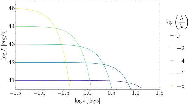
Figure 5: Example light curves based on the distribution of $\lambda/\lambda_{0}$ using the analytic methods described by Arnett (1980, 1982). Although it appears possible for the peak luminosity of a stellar collision to reach or even surpass that of a SLSNe, the extremely short duration makes it less likely that such an event could be detected. However, less luminous events which could initially be mistaken as low-luminosity supernovae could potentially be detected, especially with advances in survey technology.

4 Observed Rates

We assume that the volumetric rate of stellar collision events takes the form $R(z)=R_{0}\times f(z)$, where $R_{0}$ is the rate at redshift zero with units Mpc^-3 yr^-1, and $f(z)$ is the redshift evolution. We calculate $R_{0}$ as the product of the collision rate per galaxy with a SMBH of a certain mass and the volumetric density of galaxies with the same SMBH mass (Torrey et al., 2015). We associate each galaxy with a SMBH of mass $M_{\bullet}$ with a halo mass $M_{h}$ using the following prescription: we calculate the bulge mass associated with $M_{\bullet}$ using Eq. (2) in McConnell & Ma (2013), the corresponding total stellar mass using Fig. 1 in Bluck et al. (2014), and finally the corresponding halo mass using Eq. (2) in Moster et al. (2010). Given a specific halo mass, we then convert the mass function fit from Warren et al. (2006) into a function of redshift $z$, i.e. a function of the form $n(z)=n_{0}\times f(z)$, where $n$ is the number density of halos at a given mass and $n_{0}$ is a constant. This method gives us our redshift evolution $f(z)$, completing our calculation of $R(z)$.

We can then calculate the overall number of events of a given type by integrating over redshift,

$$\ N=\int_{0}^{z}\epsilon\left(z^{\prime}\right)\frac{4\pi R(z^{\prime})}{(1+z^{\prime})}\frac{dV_{c}}{dz^{\prime}}dz^{\prime},$$ (14)

where $dV_{c}/dz$ is the comoving volumetric element and $\epsilon(z)$ is the detection efficiency, $0\leq\epsilon(z)\leq 1$. $\epsilon(z)$ depends on multiple factors: the survey footprint and cadence, as well as what fraction of detected events can actually be distinguished. For the upcoming Large Synoptic Survey Telescope’s (LSST) Deep Drilling Field (DDF) survey, we expect that $\epsilon(z)$ will be no more than $\sim 10^{-3}$ at low redshift (and possibly much lower due to the short duration of these events), and will decline monotonically at higher redshift (Villar et al., 2018). We note that although much more observing time will be given to the Wide-Fast-Deep (WFD) survey (Ivezić et al., 2019), we expect that the average revisit time of $\sim 3$ days will be too long to identify a significant number of our events, especially at higher energies.

In figure 6, we integrate over redshift $z$ up to some value and plot $N/\epsilon$ as a function of $z$, making the simplification that $\epsilon(z)$ is a constant.

Figure 6: The cumulative number of collision events for galaxies with depletion time scales of $t_{\mathrm{D}}=10^{8},10^{9},10^{10}$ for galaxies with (a) $M_{\bullet}=10^{8}\,{M}_{\odot}$, (b) $M_{\bullet}=10^{9}\,{M}_{\odot}$, and (c) $M_{\bullet}=10^{10}\,{M}_{\odot}$. We make the simplifying assumption that the detection efficiency $\epsilon(z)$ is a constant in order to move it out of the integral in Eq. (14) (realistically, for a survey like LSST, we expect it to decline monotonically with redshift).

5 Discussion

We find that star-star collisions which release $\sim 10^{49}-10^{51}$ erg are the most common in the three host galaxies we consider, with $M_{\bullet}=10^{8},10^{9},10^{10}\,{M}_{\odot}$. Galaxies with higher-mass SMBHs are more likely to have higher-energy collisions due to the higher velocities near the center of the galaxy, but they have overall lower collision rates due to their lower stellar density. Surveys in the near future could possibly detect several tens of events like these each year (Villar et al., 2018). In addition, collisions which release upwards of $\sim 10^{53}$ erg can occur with a lower collision rate $\sim 10^{-6}$ yr^-1. These higher-energy collisions would release similar energy as SLSNe (Gal-Yam, 2012), but with the distinguishing feature of being high-metallicity events due to their occurrence at the center of a galaxy (Rich et al., 2017). Conventional SLSNe, on the other hand, are believed to show a preference for low-metallicity environments (Leloudas et al., 2015; Angus et al., 2016). Furthermore, we only expect to find these high-energy, high-velocity stellar collisions in galaxies with a SMBH with mass $M_{\bullet}\gtrsim 10^{8}\,{M}_{\odot}$, which can be used as a straightforward initial screening for these events. In addition, the most energetic collisions are most likely to take place near the SMBH, which will be an important distinguishing feature when comparing to CCSNe.

For $\lambda/\lambda_{0}<1$, which we predict represents over half of all possible collisions, the peak luminosity is roughly equal to or even greater than that from most supernovae, but the light curve is expected to decay much faster. At the most extreme values of $\lambda$ among our samples, the light curve could have a peak luminosity roughly equal to that of a SLSNe (Gal-Yam, 2019), but it would decay over 6 order of magnitude in luminosity in under 2 days, making events like these highly unlikely to be detected. However, some of the most common events we predict, with $\lambda/\lambda_{0}\sim 0.1-1$, could possibly decay slowly enough to be detected. It is possible that they would also be mistaken as low-luminosity supernovae (Zampieri et al., 2003; Pastorello et al., 2004).

Finally, we note that these stellar collisions will likely create a stream of debris that would partly accrete onto the SMBH, creating an accretion flare. This accretion flare may resemble a tidal disruption event (TDE) (Loeb & Ulmer, 1997; Gezari, 2021; Dai et al., 2021; Mockler & Ramirez-Ruiz, 2021), even though the black hole is too massive for a TDE. The stellar explosion we have described in this work will be a precursor flare to the black hole accretion flare. We expect that the center of mass of the debris from the stellar collision would follow a trajectory consistent with momentum conservation after the collision and will also spread in its rest frame following the explosion dynamics that we consider. Altogether it would resemble a stream of gas that gets thicker over time. The accretion rate on the SMBH could be super-Eddington as in the case of TDEs and make the black hole shine around or above the Eddington luminosity, $L_{E}=1.4\times 10^{46}\,(M_{\bullet}/10^{8}\,{M}_{\odot})$ erg/s. This luminosity is far larger than we calculated for the collision itself and could be much easier to detect. The details of the accretion flare will be sensitive to the distance of the collision from the SMBH and the velocities and masses upon impact. We leave the numerical and analytical study of this problem to future work (Hu & Loeb 2021, in prep).

6 Acknowledgments

This work was supported by the Black Hole Initiative at Harvard University, which is funded by grants from the John Templeton Foundation and the Gordon and Betty Moore Foundation.

References

- Angus et al. (2016) Angus, C. R., Levan, A. J., Perley, D. A., et al. 2016, MNRAS, 458, 84, doi: 10.1093/mnras/stw063
- Arcavi et al. (2017) Arcavi, I., Howell, D. A., Kasen, D., et al. 2017, Nature, 551, 210, doi: 10.1038/nature24030
- Arnett (1996) Arnett, D. 1996, Supernovae and Nucleosynthesis: An Investigation of the History of Matter from the Big Bang to the Present
- Arnett (1980) Arnett, W. D. 1980, ApJ, 237, 541, doi: 10.1086/157898
- Arnett (1982) —. 1982, ApJ, 253, 785, doi: 10.1086/159681
- Balberg et al. (2013) Balberg, S., Sari, R., & Loeb, A. 2013, MNRAS, 434, L26, doi: 10.1093/mnrasl/slt071
- Barkat et al. (1967) Barkat, Z., Rakavy, G., & Sack, N. 1967, Phys. Rev. Lett., 18, 379, doi: 10.1103/PhysRevLett.18.379
- Behroozi et al. (2019) Behroozi, P., Wechsler, R. H., Hearin, A. P., & Conroy, C. 2019, Monthly Notices of the Royal Astronomical Society, 488, 3143, doi: 10.1093/mnras/stz1182
- Bellm (2014) Bellm, E. 2014, in The Third Hot-wiring the Transient Universe Workshop, ed. P. R. Wozniak, M. J. Graham, A. A. Mahabal, & R. Seaman, 27–33. https://arxiv.org/abs/1410.8185
- Bluck et al. (2014) Bluck, A. F. L., Mendel, J. T., Ellison, S. L., et al. 2014, Monthly Notices of the Royal Astronomical Society, 441, 599, doi: 10.1093/mnras/stu594
- Bose et al. (2018) Bose, S., Dong, S., Pastorello, A., et al. 2018, ApJ, 853, 57, doi: 10.3847/1538-4357/aaa298
- Colgate (1974) Colgate, S. A. 1974, ApJ, 187, 333, doi: 10.1086/152632
- Dai et al. (2021) Dai, J. L., Lodato, G., & Cheng, R. 2021, Space Sci. Rev., 217, 12, doi: 10.1007/s11214-020-00747-x
- Demircan & Kahraman (1991) Demircan, O., & Kahraman, G. 1991, Astrophysics and Space Science, 181, 313, doi: 10.1007/BF00639097
- Dong et al. (2020) Dong, Y., Valenti, S., Bostroem, K. A., et al. 2020, ApJ, 906, 56, doi: 10.3847/1538-4357/abc417
- Frieman et al. (2008) Frieman, J. A., Bassett, B., Becker, A., et al. 2008, AJ, 135, 338, doi: 10.1088/0004-6256/135/1/338
- Frohmaier et al. (2021) Frohmaier, C., Angus, C. R., Vincenzi, M., et al. 2021, MNRAS, 500, 5142, doi: 10.1093/mnras/staa3607
- Gal-Yam (2012) Gal-Yam, A. 2012, Science, 337, 927, doi: 10.1126/science.1203601
- Gal-Yam (2019) Gal-Yam, A. 2019, ARA&A, 57, 305, doi: 10.1146/annurev-astro-081817-051819
- Gezari (2021) Gezari, S. 2021, arXiv e-prints, arXiv:2104.14580. https://arxiv.org/abs/2104.14580
- Graham (2012) Graham, A. W. 2012, The Astrophysical Journal, 746, 113, doi: 10.1088/0004-637X/746/1/113
- Guillochon et al. (2017) Guillochon, J., Parrent, J., Kelley, L. Z., & Margutti, R. 2017, ApJ, 835, 64, doi: 10.3847/1538-4357/835/1/64
- Gutiérrez et al. (2020) Gutiérrez, C. P., Sullivan, M., Martinez, L., et al. 2020, MNRAS, 496, 95, doi: 10.1093/mnras/staa1452
- Hernquist (1990) Hernquist, L. 1990, ApJ, 356, 359, doi: 10.1086/168845
- Hillebrandt & Niemeyer (2000) Hillebrandt, W., & Niemeyer, J. C. 2000, ARA&A, 38, 191, doi: 10.1146/annurev.astro.38.1.191
- Ivezić et al. (2019) Ivezić, Ž., Kahn, S. M., Tyson, J. A., et al. 2019, ApJ, 873, 111, doi: 10.3847/1538-4357/ab042c
- Kasliwal et al. (2010) Kasliwal, M. M., Kulkarni, S. R., Gal-Yam, A., et al. 2010, ApJ, 723, L98, doi: 10.1088/2041-8205/723/1/L98
- Kesden (2012) Kesden, M. 2012, Phys. Rev. D, 85, 024037, doi: 10.1103/PhysRevD.85.024037
- Khatami & Kasen (2019) Khatami, D. K., & Kasen, D. N. 2019, The Astrophysical Journal, 878, 56, doi: 10.3847/1538-4357/ab1f09
- Leloudas et al. (2015) Leloudas, G., Schulze, S., Krühler, T., et al. 2015, MNRAS, 449, 917, doi: 10.1093/mnras/stv320
- Loeb & Ulmer (1997) Loeb, A., & Ulmer, A. 1997, ApJ, 489, 573, doi: 10.1086/304814
- Matzner & McKee (1999) Matzner, C. D., & McKee, C. F. 1999, ApJ, 510, 379, doi: 10.1086/306571
- McConnell & Ma (2013) McConnell, N. J., & Ma, C.-P. 2013, ApJ, 764, 184, doi: 10.1088/0004-637X/764/2/184
- Mockler & Ramirez-Ruiz (2021) Mockler, B., & Ramirez-Ruiz, E. 2021, ApJ, 906, 101, doi: 10.3847/1538-4357/abc955
- Moster et al. (2010) Moster, B. P., Somerville, R. S., Maulbetsch, C., et al. 2010, ApJ, 710, 903, doi: 10.1088/0004-637X/710/2/903
- Nakaoka et al. (2019) Nakaoka, T., Moriya, T. J., Tanaka, M., et al. 2019, The Astrophysical Journal, 875, 76, doi: 10.3847/1538-4357/ab0dfe
- Nakar & Sari (2010) Nakar, E., & Sari, R. 2010, ApJ, 725, 904, doi: 10.1088/0004-637X/725/1/904
- Pastorello et al. (2004) Pastorello, A., Zampieri, L., Turatto, M., et al. 2004, Monthly Notices of the Royal Astronomical Society, 347, 74, doi: 10.1111/j.1365-2966.2004.07173.x
- Perets et al. (2010) Perets, H. B., Gal-Yam, A., Mazzali, P. A., et al. 2010, Nature, 465, 322, doi: 10.1038/nature09056
- Prentice et al. (2018) Prentice, S. J., Maguire, K., Smartt, S. J., et al. 2018, ApJ, 865, L3, doi: 10.3847/2041-8213/aadd90
- Rau et al. (2009) Rau, A., Kulkarni, S. R., Law, N. M., et al. 2009, PASP, 121, 1334, doi: 10.1086/605911
- Rich et al. (2017) Rich, R. M., Ryde, N., Thorsbro, B., et al. 2017, AJ, 154, 239, doi: 10.3847/1538-3881/aa970a
- Rubin & Loeb (2011) Rubin, D., & Loeb, A. 2011, Advances in Astronomy, 2011, 174105, doi: 10.1155/2011/174105
- Sahu et al. (2020) Sahu, N., Graham, A. W., & Davis, B. L. 2020, The Astrophysical Journal, 903, 97, doi: 10.3847/1538-4357/abb675
- Scolnic et al. (2018) Scolnic, D. M., Jones, D. O., Rest, A., et al. 2018, ApJ, 859, 101, doi: 10.3847/1538-4357/aab9bb
- Smartt (2009) Smartt, S. J. 2009, ARA&A, 47, 63, doi: 10.1146/annurev-astro-082708-101737
- Stone et al. (2019) Stone, N. C., Kesden, M., Cheng, R. M., & van Velzen, S. 2019, General Relativity and Gravitation, 51, 30, doi: 10.1007/s10714-019-2510-9
- Taddia et al. (2016) Taddia, F., Sollerman, J., Fremling, C., et al. 2016, A&A, 588, A5, doi: 10.1051/0004-6361/201527811
- Tampo et al. (2020) Tampo, Y., Tanaka, M., Maeda, K., et al. 2020, ApJ, 894, 27, doi: 10.3847/1538-4357/ab7ccc
- Torrey et al. (2015) Torrey, P., Wellons, S., Machado, F., et al. 2015, Monthly Notices of the Royal Astronomical Society, 454, 2770, doi: 10.1093/mnras/stv1986
- Tremaine et al. (1994) Tremaine, S., Richstone, D. O., Byun, Y.-I., et al. 1994, The Astronomical Journal, 107, 634, doi: 10.1086/116883
- Villar et al. (2018) Villar, V. A., Nicholl, M., & Berger, E. 2018, ApJ, 869, 166, doi: 10.3847/1538-4357/aaee6a
- Warren et al. (2006) Warren, M. S., Abazajian, K., Holz, D. E., & Teodoro, L. 2006, ApJ, 646, 881, doi: 10.1086/504962
- Woosley & Weaver (1995) Woosley, S. E., & Weaver, T. A. 1995, ApJS, 101, 181, doi: 10.1086/192237
- Zampieri et al. (2003) Zampieri, L., Pastorello, A., Turatto, M., et al. 2003, Monthly Notices of the Royal Astronomical Society, 338, 711, doi: 10.1046/j.1365-8711.2003.06082.x